2.1. Marine radar data pre-processing

To apply deep learning to marine radar images, we first compiled the images into a dataset. This was then augmented to improve detection. Subsequently, we performed annotation of typical targets.

Before target detection, a typical radar target dataset should be constructed. We selected real-time ship radar images referenced by duty officers or pilots from vessels in different narrow channels as samples for typical target detection. After the vessels docked, we used the Voyage Data Recorder (VDR) monitor to acquire ENC data and marine radar images from the corresponding narrow channel over the previous 12 hours.

We used a data augmentation method to avoid overfitting and increase data availability during training as the obtained dataset was small for deep learning (Wu et al., Reference Wu, Xu, Zhu and Guo2017). This data augmentation approach consists of geometrical transformations, such as horizontal flipping, resizing, rotation and cropping to generate synthetic images.

Our team was supported by ten senior seafarers who manually annotated typical targets from marine radar images using bounding boxes and then labelled their classes. These annotations were verified with reference to the chart, and typical targets were placed at the centre of the bounding boxes.

2.2. Target detection using neural networks

For efficient and robust marine radar typical target detection, we selected two models with strong generalisation capability, namely, Faster Region-based CNN (Faster R-CNN) and Region-based Fully Convolutional Network (R-FCN) (Dai et al., Reference Dai, Li, He, Sun, Chen, Gong and Tie2016). In addition, we selected the Oxford Visual Geometry Group (VGG) VGG-16 deep CNN (VGG-16) and the 101-layer residual neural network (ResNet-101) in imageNet Large Scale Visual Recognition Challenge (He et al., Reference He, Zhang, Ren and Sun2016; Simonyan and Zisserman, Reference Simonyan and Zisserman2015) with fast training and testing, respectively, to be the feature extractors.

2.2.1. Faster R-CNN

Faster R-CNN performs detection in two stages. In the first stage, a Region Proposal Network (RPN) accepts a marine radar image as input and extracts its features to indicate the subsequent detection model of the regions it should analyse. We slid a small network over the obtained convolutional feature map of the radar image to generate region proposals. Each feature is mapped into a lower-dimensional feature, which is fed into box-regression and box-classification layers. To train the RPN, we assigned a binary class label determined from the intersection-over-union overlap compared to a threshold with any ground-truth box to each anchor indicating whether it is an object. The loss function for the image is defined as:

(1)$$L(\{ p_i\},\{ t_i\} ) = \displaystyle{1 \over {N_{cls}}}\sum\limits_i {L_{cls}} (p_i + p_i^* ) + \lambda \displaystyle{1 \over N}\sum\limits_i {p_i^* } L_{reg}(t_i,t_i^* )$$

where i is the anchor index in a mini-batch, p _i is the probability of anchor i being an object, t _i is a vector representing the four parameterised coordinates of the predicted bounding box, t _i* is the vector of the ground-truth box associated with a positive anchor, and λ is a balancing weight (Ren et al., Reference Ren, He, Girshick and Sun2015). The classification loss is the log loss over two classes as follows:

(2)$$L_{cls}\lpar {p_i,p_i^* } \rpar = \log [p_ip_i^* + (1-p_i^* )(1-p_i)]$$

and the regression loss is given by:

(3)$$L_{reg}\lpar {t_i,t_i^* } \rpar = \left\{ {\matrix{ {0\cdot 5{(t_i-t_i^* )}^2} \hfill & {if\;\vert {t_i-t_i^* } \vert < 1} \hfill \cr {\vert {t_i-t_i^* } \vert -0\cdot 5} \hfill & {otherwise} \hfill \cr } } \right..$$

For bounding box regression, we adopted the parameterisation of the four coordinates as follows:

(4)$$\eqalign{t_x &= (x_p-x_a)/w_a,t_y = (y_p-y_a)/h_a \cr t_w &= \log (w_p/w_a),\quad t_h = \log (h_p/h_a) \cr t_x^* & = (x^*-x_a)/w_a,t_y^* = (y^*-y_a)/h_a \cr t_w^* &= \log (w^*/w_a),\quad t_h^* = \log (h^*/h_a)}$$

where x _p, x _a and x* correspond to the predicted box, anchor box and ground-truth box, respectively (likewise for w _p, y _p, h _p). Variables x _p, y _p, w _p and h _p denote the two centre coordinates of the bounding box and its width and height. The RPN and subsequent detection are illustrated in Figure 1.

Figure 1. Diagram of the RPN architecture (left) and example of detections using RPN outcomes (right).

In the second stage, the box proposals are used to detect marine radar image features from the feature map. These features are fed into the remaining layers of the feature extractor for predicting the class probability and bounding box for each proposal.

The entire process is implemented on a unified network as shown in Figure 2, enabling sharing of full-image convolutional features with the detection network and significantly reducing the number of weights for simplifying and speeding-up training.

Figure 2. Block diagram of Faster R-CNN (ROI, region of interest).

2.2.2. R-FCN

The R-FCN illustrated in Figure 3 uses convolution for prediction and then performs region-of-interest pooling. Adding location information before pooling prevents the fully convolutional network from losing such information and specifying different score maps allows detection of different locations of the target. After pooling, the score maps obtained from different locations can be combined to reconstruct the original location information, whereas the fully convolutional structure reduces training time.

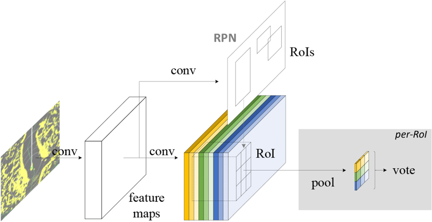
Figure 3. R-FCN with fully convolutional network.

We evaluated the performance of the models using the mean average precision (Everingham et al., Reference Everingham, van Gool, Williams, Winn and Zisserman2010). The average precision is the area under the precision (p)–recall (r) curve of the detection task, and its mean is computed over all the classes in a task. The average precision and mean average precision are respectively given by:

(5)$$\eqalign{AP &= \sum\limits_i^{n_d} {p_i} \Delta r \cr mAP &= \displaystyle{1 \over C}\sum\limits_{C = 1}^C {AP_C} }$$

The average precision AP is a dimensionless quantity and integrates both the precision and recall indicators, which are commonly used to measure the ability of neural networks to detect targets, with higher values indicating the model more suitable for the data set. Likewise, the mean average precision mAP is the average precision (including background) of each object, which is used to measure the target detection ability of the model for a category of targets.

2.3. Transfer learning

We used transfer learning to fine-tune the detection model as the employed dataset is small. In fact, modern object detection considers a large number of data samples and over a thousand class labels. Then, the hidden layers in a CNN provide distinct feature representations, with lower layers providing general feature extraction and higher layers providing more specific information about the intended task (Dai et al., Reference Dai, Li, He, Sun, Chen, Gong and Tie2016). For instance, lower layers would be edge detectors, whereas higher layers provide more specific representations belonging to the input image. Therefore, generalisation is provided by feature extraction and representation of lower layers and fine-tuning of the specific problem is provided by higher layers. The transfer learning employed in this study to improve detection is illustrated in Figure 4. In this study, we used a dataset available online, namely UC Merced Land Use Dataset with 21 object classes (Yang and Newsam, Reference Yang and Newsam2010) to perform pre-training. The main purpose was to guide the lower layers of the network to extract features in the proper direction. Then, fine-tuning was performed on higher layers using the radar data set generated in the present study.

Figure 4. Diagram of transfer learning to improve target detection.

3.1. Scaling and display area of ENC

The coordinate systems of the ENC and corresponding radar images are different, leading to superposition errors, which can be mitigated by performing real-time coordinate transformations. For the ENC, the projection mode defaults to the Mercator projection as this type of projection is simpler to calculate and yields higher accuracy in a small scanning range than similar methods. We used the Mercator projection by considering the scanning range of the radar, which is usually within six nautical miles when ships sail in confined waters.

The effect of the curvature of the Earth between the radar detection coordinate system and the Mercator coordinate system can be ignored as this value is too small compared to the radius of the Earth. When the range is small, the detection distance of the radar is approximately equal to the geographical distance considering the curvature of the earth. The conversion of the geodetic coordinate system into Mercator projection proceeds as follows (Yang et al., Reference Yang, Dou and Zheng2010):

(6)$$\eqalign{& \left\{ {\matrix{ {x_m = r_0q} \hfill \cr {y_m = r_0\lambda } \hfill \cr } } \right. \cr & r_0 = \displaystyle{\alpha \over {\sqrt {1-e^2\sin \varphi _r} }} \times \cos \varphi _r \cr & q = \ln {\rm tan}\;\left( {\displaystyle{\pi \over 4} + \displaystyle{\varphi \over 0}} \right)-\displaystyle{e \over 2}\ln \displaystyle{{1 + e\sin \varphi } \over {1-e\sin \varphi }}}$$

where x _m and y _m are the Mercator Cartesian coordinates, λ and φ are the longitude and latitude, respectively, α is the major axis of the Earth's ellipsoid, e is the first eccentricity of the Earth, φ _r is the reference dimension, q is the equivalent dimension, and r ₀ is the radius of the base circle of the latitude.

According to the projection transformation of chart pixels, the latitude and longitude of the radar scan can be obtained as:

(7)$$\left\{ {\matrix{ {\lpar {\lambda_{\min },\lambda_{\min }} \rpar = \phi_{org}^{-1} \;\lpar {\phi \lpar {\lambda_0,\varphi_0} \rpar -\lpar {L,L} \rpar } \rpar } \hfill \cr {\lpar {\lambda_{\max },\lambda_{\max }} \rpar = \phi_{org}^{-1} \;\lpar {\phi \lpar {\lambda_0,\varphi_0} \rpar + \lpar {L,L} \rpar } \rpar } \hfill \cr } } \right.$$

where λ₀ and φ ₀ are the longitude and latitude of the radar centre, respectively, (λ_min, φ _min) and (λ_max, φ _max) are the longitude and Lattitude ranges of the radar scanning, respectively, ϕ(λ₀, φ ₀) is the longitude and Lattitude of the radar centre in Cartesian coordinates with ϕ being the map for Mercator projections, respectively, ϕ ⁻¹ is the inverse of the Mercator map for chart projection, and L is the detection range of the radar. Then, we searched the area of the ENC to be registered using the results obtained.

In terms of the registration, the ENC and marine radar scales must be consistent. Modifying the radar scale is achieved by several variation ranges, whereas ENC data can be arbitrarily set to the desired scale. Therefore, we matched the electronic chart to radar data (Yang et al., Reference Yang, Dou and Zheng2010). A radar image scale and the display scale of the ENC are determined by:

(8)$$\eqalign{\displaystyle{1 \over {S_r}} &= \displaystyle{{c \times d} \over R} \cr z &= \displaystyle{{\lpar {c \times d \times s_0} \rpar } \over R}}$$

where R is the detection radius of the radar, c pixels at distance d are contained in the radius scan line, and 1/s _r is the original scale of the radar. However, the remaining area, excluding the radar image area, is displayed in black on the radar display screen. Thus, 1/s _r can also be regarded as the scale of the external square of the radar circular image. 1/s ₀ is the original scale of the ENC, and z is the scaling parameter of the ENC.

According to the azimuth and distance of the corners of the bounding boxes obtained from radar target detection with respect to the registration reference point, areas outside the bounding box in the ENC are treated as background, whereas the area within the bounding box of the ENC data and radar image is the Registration Interest Area (RIA).

3.2. RIA processing

3.2.1. Filtering algorithm

Unlike registration based on entire radar images, filtering and parameter selection considering only RIAs can be more accurate for extracting the edges. For enhanced applicability, we consider real-time fusion and adaptive mean filtering, which is expressed as:

(9)$$K(x) = c_k\;k\;\left( {{\left\| x \right\|}^2} \right)$$

where x is a pixel in the plane, c _k is a constant greater than 0, k (x) satisfies ∫k(x)dr < 0, and K(x) is a kernel function. The kernel density estimate is given by:

(10)$$\eqalign{f(x) &= \displaystyle{1 \over n}\sum\limits_{i = 1}^n {K_{\rm H}} (x-x_i) \cr K_{\rm H}(x) &= \vert H \vert ^{-1/2}K\lpar {H^{-1/2}x} \rpar }$$

where H = h ²I. Simplifying the density function, we obtain:

(11)$$f(x) = \displaystyle{1 \over {nh^d}}\sum\limits_{i = 1}^n k \left( {\left\| {\displaystyle{{x-x_i} \over h}} \right\| } \right)$$

whose gradient is given by:

(12)$$\nabla f(x) = \displaystyle{{2C_k} \over {nh^{d + 2}}}\sum\limits_{i = 1}^n {k^{\prime}} \left( {{\left\| {\displaystyle{{x-x_i} \over h}} \right\| }^2} \right).$$

Assuming g(x) = −k ^′(x), $G\lpar x\rpar = c_{k}g\ \lpar \Vert x\Vert^{2}\rpar $, and G(x) is the opacification function of K(x), we obtain:

(13)$$\eqalign{\nabla f(x) &= \displaystyle{{2c_k} \over {nh^{d + 2}}}\left[ {\sum\limits_{i = 1}^n \; g\;{\left( {\left\| {\displaystyle{{x-x_i} \over h}} \right\| } \right)}^2} \right]\left[ {\displaystyle{{\sum\limits_{i = 1}^n {x_i} g\;{\left( {\left\| {\displaystyle{{x-x_i} \over h}} \right\| } \right)}^2} \over {\sum\limits_{i = 1}^n \; g\;{\left( {\left\| {\displaystyle{{x-x_i} \over h}} \right\|} \right)}^2}}-x} \right] \cr & = \displaystyle{{2c_k} \over {nh^{d + 2}}}\left[ {\sum\limits_{i = 1}^n \; g\;{\left( {\left\| {\displaystyle{{x-x_i} \over h}} \right\|} \right)}^2} \right]\lsqb {m_h\;(x)-x} \rsqb }$$

with m _h(x) being the weighted average of the sample points used to update the search area with radius h and m _h (x) − x being a drift vector, which terminates the iteration process when it is below a certain tolerance level.

3.2.2. Binarization

To avoid intensive processing of colour images, we binarized greyscale images using the method by Otsu (Reference Otsu1979) to prevent disparity between the RIA foreground and the background size ratio. This method adaptively searches for a threshold according to the characteristics of the image and converts a greyscale image into a binary one. The transformation can be expressed as:

(14)$$\eqalign{u &= w_0*u_0 + w_1*u_1 \cr g(t) &= w_0(u_0-u)^2 + w_1(u_1-u)^2}$$

where w ₀ is the ratio of foreground to image with u ₀ being its average greyscale value and w ₁ is the ratio of background to image with u ₁ being its average greyscale value. The highest variance g maximises the foreground and background difference, and the corresponding threshold t is the optimum.

3.2.3. Morphological processing

Binarization may produce some isolated noise pixels besides the foreground target, affecting its integrity. We performed noise removal by applying corrosion, expansion, opening, and closing, which can be expressed using the standard set theory as:

(15)$$\eqalign{A\Theta B &= \lcub {w\in Z + b\in A,b\in B} \rcub \cr A\oplus B &= \lcub {w\in Z = a + b,a\in A,b\in B} \rcub \cr A \circ B &= (A\Theta B)\oplus B \cr A \bullet B &= (A\oplus B)\Theta B}$$

where Z represents the foreground, w is a pixel at different positions in the foreground image, and a and b are members of structural element sets A and B, respectively.

We used the improved canny operator (Othman and Abdullah, Reference Othman and Abdullah2018) to extract the edge of the radar image and boundary of the echoes in the RIAs:

(16)$$\eqalign{ E_x &= \displaystyle{{\partial P} \over {\partial x}}*f(x,y)\quad E_y = \displaystyle{{\partial P} \over {\partial y}}*f(x,y) \cr A(i,j) &= \sqrt {E_x^2 (i,j) + E_y^2 (i,j)} \cr a(i,j) &= \arctan \left( {\displaystyle{{E_x\;(x,y)} \over {E_y\;(x,y)}}} \right)}$$

where P(x, y) is a two-dimensional Gaussian function, f(x, y) is the image data, A(i, j) is the edge feature of point (i, j) in the image, and a(i, j) is the normal vector of the image at point (i, j). Figure 5 illustrates the complete image processing for an RIA.

Figure 5. Image processing of RIA. (a) RIA; (b) Filtering and Binarization; (c) Morphological processing; (d) Canny.

3.3. Image registration

Image registration can be based on transformations of greyscale images, features and domain. Considering the notable divergence between marine radar images and ENC, we used a feature-based affine transformation for their fusion. Three or more reference points should be selected for the transformation, and its principle can be expressed as:

(17)$$\left[ {\matrix{ {x_i^{\prime} } \cr {y_i^{\prime} } \cr } } \right] = k^{\prime}\left[ {\matrix{ {\cos \theta } & {\sin \theta } \cr {-\sin \theta } & {\cos \theta } \cr } } \right]\left[ {\matrix{ {x_i} \cr {y_i} \cr } } \right] + \left[ {\matrix{ {x_0} \cr {y_0} \cr } } \right]$$

where (x _i, y _i) are the coordinates of a pixel in the ENC, k ^′, θ, x _o and y _o are parameters for the affine transformation, where θ corresponds to the image rotation, k is a scale factor and x ₀ and y ₀ correspond to the image shift. Thus, we obtain:

(18)$$\left\{ {\matrix{ {x_i^{\prime} = a_{11}x_i + a_{12}y_i + a_{13}} \hfill \cr {y_i^{\prime} = a_{21}x_i + a_{22}y_i + a_{23}} \hfill \cr } } \right.$$

with a ₁₁ = a ₂₂ = k ^′cosθ, a ₁₃ = x _o, a ₁₂ = −a ₂₁ = k ^′sinθ, and a ₂₃ = y _o.

Therefore, correlating radar images with ENC data requires at least three pairs of reference points with accurate correspondence to determine the transformation parameters. The accuracy of the reference points directly determines the fusion outcome. After the transformation, however, some deformation may occur, but it is generally negligible. On the other hand, if the deformation undermines fusion, then according to “the display of radar information shall have priority” from IEC 62388 (2013), priority should be given to the display of radar images.

To determine the reference points for registration, we considered various aspects. After target detection from the radar image, targets with small sizes and inconspicuous shapes may interfere with the detection results, as registration is less effective for small objects such as buoys. However, according to the International Convention on Standards of Training, Certification and Watchkeeping for Seafarers, when ships are sailing along the coast in crowded waters, the crew should check the position of the ship at appropriate intervals through independent positioning methods, and reference objects are mainly used for navigation. Therefore, small reference objects that can accurately correspond to the ENC goal should not be ignored. Consequently, pixels between the radar image and ENC are suitable as registration reference points.

Depending on the target resolution of the radar, manual selection of registration reference points cannot be performed on large ranges. Therefore, we implemented the automatic registration algorithm, illustrated in Figure 6, which focused on objects that perform well in target detection as reference points for registration. The algorithm first locates a pair of accurate reference points on the ENC and radar images whose respective coordinates are (x ₁, y ₁) and $\lpar x_{1}^{\prime}\comma \; y_{1}^{\prime}\rpar $. When two or more bounding boxes are found, a ray is emitted from (x ₁, y ₁) and $\lpar x_{1}^{\prime}\comma \; y_{1}^{\prime}\rpar $ to the geometric centre of the RIA in the ENC and radar images to acquire two or more groups of coordinates in front of the radar echo edge. If there is only one bounding box, a specific angle on the bow is selected, emitting two rays to the areas around (x ₁, y ₁) and $\lpar x_{1}^{\prime}\comma \; y_{1}^{\prime}\rpar $ to obtain the coordinates of the two registration reference points.

Figure 6. Complete process for automatic registration from detected typical targets. (a) Detection result; (b) Binarization; (c) Morphological processing; (d) Canny; (e) Registration.

4.1. Typical target detection

We leveraged the UC Merced Land Use Dataset with 21 object classes (Yang and Newsam, Reference Yang and Newsam2010) as a dataset sample for pre-training the network toward the problem domain of specific object classes for detection. The annotated typical target dataset (ENC data and marine radar images acquired from the voyage data recorder monitor) was used to fine-tune the pre-trained model using transfer learning. We used stochastic gradient descent with momentum and weight decay of 0·9 and 0·0005, respectively. The initial learning rate of 0·001 was divided by 10 using stepdown every 12,000 iterations. For the RPN in the Faster R-CNN and R-FCN, we set the batch size to 256.

Table 1 lists the performance of the Faster R-CNN and R-FCN in the data set we constructed. Both detection performances for typical marine radar targets are not ideal. However, the R-FCN performed better than the Faster R-CNN as the mAP of the R-FCN is higher than that of the Faster R-CNN; a detection model with a higher mAP value can classify the target data set considering the precision and recall overall. Thus, the R-FCN is considered more suitable to perform the detection task in our data set efficiently. From these results, we determined that various factors should be considered for typical radar target detection. First, radar information from different target types may be very similar, thus undermining the detection accuracy. Figure 7 shows examples of indistinguishable objects, namely a shoal (Figure 7(b)) and a breakwater (Figure 7(d)).

Table 1. Detection result of Faster R-CNN and R-FCN for typical radar target.

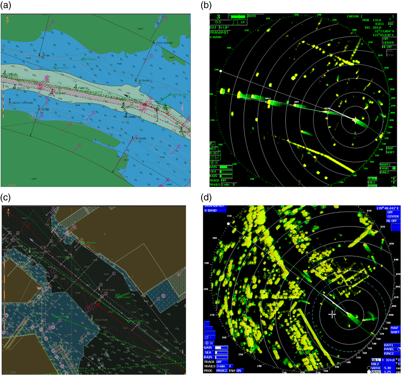
Figure 7. Typical target with undistinguishable echoes: (a) ENC of a shoal; (b) radar echoes of a shoal; (c) ENC of a breakwater; (d) Civil Marine Radar (CMR) echoes of a breakwater.

In addition, targets with small sizes and inconspicuous shapes may interfere with the detection results. In fact, such targets produce a low average precision that undermines detection. Furthermore, although the position of the ship is stable, and its geometric shape is regular with strong capability to reflect Civil Marine Radar (CMR) echoes, the average precision of the vessel is low; furthermore, there will be leakage detection and error detection, as illustrated in Figure 8. Therefore, ships cannot be used as reference points for automatic registration.

Figure 8. Target detection of ships showing detection omission (a) without and (b) with radar persistence.

To improve the detection performance, we considered typical targets in the radar images with different characteristics and trained different models to reduce the detection classes and avoid similarity among different targets. For example, we considered the waters near the Yangtze River estuary (Figure 9). According to the Shanghai Gang sailing direction, arriving ships mostly rely on lights and lightships for positioning and navigation. However, it is difficult to distinguish lighthouses and lightships from a large number of densely anchored ships. In addition, the position and shape of echoes from smooth beach shorelines and mudflats can change with tide diversification. Moreover, radar images usually do not produce notable distinctions between steep and smooth beach shorelines, which are thus not suitable as reference points for registration and navigation. In these types of waters, echo-stable buildings are preferred as typical targets such as breakwaters and quayside edges, as shown in Figure 9. When these targets were used for the R-FCN, we obtained better detection performance. Specifically, target detection in the waters of the Yangtze River and waters near the Kobe Port estuary yielded average precision for the breakwater of up to 0·4372, which is higher compared to using other targets.

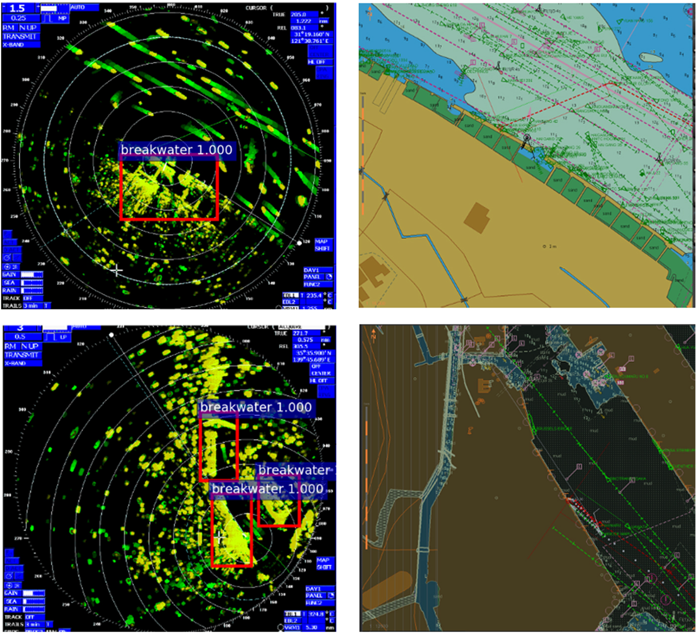
Figure 9. Breakwater selected as typical target in the area of the Yangtze river and Kobe port.

We also verified the feasibility of the R-FCN in the inland waters near the Caledon port, Vietnam and the results obtained are listed in Table 2 and shown in Figure 10. The detection performance notably improved with a mAP of 0·5178, which is significantly higher than the values previously obtained (0·2973 and 0·3649). This indicates that reducing the classification category of the target helps to improve the target detection performance of the model after considering the precision and recall rate.

Table 2. Detection of typical targets from multiple radar in waters near the Port of Caledon, Vietnam.

Figure 10. Detection of typical targets near the Port of Caledon, Vietnam.

4.2. Data fusion

The affine transformation parameters, k, θ, x _o, and y _o in Equation (17) were determined to perform fusion simulations on ENC data and CMR images at intervals of 5 min. The results are shown in Figure 11.

Figure 11. Using fixed parameter to perform data fusion of ENC and radar images every five minutes.

The algorithm yields a suitable performance because fusion of the shorelines from the ENC and radar images coincide. Moreover, the shoreline and shoal are separated in Figures 12(a) and 12(b) without loss of radar information. The image details show successful fusion by the consistent position of the land in Figure 11(a) and that of the buoys in Figures 12(a)–(c). Thus, image fusion of ENC and marine radar images can be performed even without the identification of accurate feature points.

Figure 12. Image fusion using reference points on the left and right of the ship. (a) ENC; (b) CMR image; (c) Binarization; (d) Morphological; (e1) Left side of ship; (e2) Right side of ship.

We executed training and registration using a Nvidia GeForce GTX 1080 GPU and Intel Core i5–7 processors. With this equipment, the average time for target detection on a single test image was 0·15 s, and registration was completed within 0·5 s, which is below the maximum update rate of the marine radar antenna (48 rpm), suggesting that the proposed algorithm satisfies the requirement for real-time performance.

The success of the registration algorithm depends on the quality of marine radar image processing. Moreover, if the radar detects contiguous objects for reference points near the range, these objects will cause pixel adhesion, and the canny operator cannot extract the edge features of these objects. We performed a simulation to demonstrate this situation. As shown in Figure 12(e2), the shoreline on the left side is steep without occlusion from other objects. However, the shoreline on the right of the ship is covered by a building. Taking the shoreline on the left and right of the ship as RIAs to perform automatic registration with the corresponding reference points yields the results shown in Figure 12.

Fusion using the RIA from the left of the ship successfully matches the shoreline and the bridge, but that from the right of the ship fails. The failure is caused by limitations in the working principle and performance of a CMR. Even with human assessment, it is difficult to find pixels that can accurately correspond to the ENC position among many erratic pixels. This complicates the search for registration reference points in such areas. Therefore, registration reference points in the RIA should be searched only when no object interference occurs.

Now, consider the case when the ship is being used as the reference point and the GNSS is giving a large error, thus drastically undermining fusion. In this case, achieving fusion demands reference points other than the ship. For instance, if the buoy detected by radar with clear echoes and stable position on the ENC is used as a registration reference point for fusion, the algorithm yields the result shown in Figure 13.

Figure 13. Data fusion using other reference points detected by radar under large error of the ship GNSS. (a) ENC; (b) Typical target detection; (c) Binarization; (d) Morphological; (e) Canny operator; (f) Auto Registration Algorithm; (g) Registration.

The automatic fusion of ENC data and marine radar image is realised using the buoy echo detected by the radar, disregarding information on the ship position. The fusion results show that the ship position on the radar is consistent with the GNSS signal on the ENC, and the radar echo of the shoreline is accurately integrated with ENC data, verifying the high performance of the proposed algorithm under this scenario.