


1. Introduction
Knots, closed curves in three-dimensional space in mathematical language, have been extensively studied in the physical and biological sciences (see Kauffman Reference Kauffman2001; Berger et al. Reference Berger, Ricca, Kauffman, Khesin, Moffatt and Sumners2009). Knotted structures arise in various systems, including vortex filaments in hydrodynamic (HD) flows (e.g. Kleckner & Irvine Reference Kleckner and Irvine2013), long DNA and polymer molecules (e.g. Orlandini & Whittington Reference Orlandini and Whittington2007; Stolz et al. Reference Stolz, Yoshida, Brasher, Flanner, Ishihara, Sherratt, Shimokawa and Vazquez2017; Klotz, Soh & Doyle Reference Klotz, Soh and Doyle2018), topological defects in liquid crystals (e.g. Tkalec et al. Reference Tkalec, Ravnik, Čopar, Žumer and Muševič2011) and knot solitons in Bose–Einstein condensates (e.g. Hall et al. Reference Hall, Ray, Tiurev, Ruokokoski, Gheorghe and Möttönen2016). In particular, magnetic knots have been extensively reported in magnetohydrodynamic (MHD) flows (e.g. Moffatt & Ricca Reference Moffatt and Ricca1992; Arrayás, Bouwmeester & Trueba Reference Arrayás, Bouwmeester and Trueba2017; Smiet et al. Reference Smiet, Thompson, Bouwmeester and Bouwmeester2017; Knizhnik, Linton & Devore Reference Knizhnik, Linton and Devore2018) and magnetic torus knots are often used in model problems (see Candelaresi & Brandenburg Reference Candelaresi and Brandenburg2011; Arrayás & Trueba Reference Arrayás and Trueba2014; Smiet et al. Reference Smiet, Candelaresi, Thompson, Swearngin, Dalhuisen and Bouwmeester2015; Xiong & Yang Reference Xiong and Yang2020).
Magnetic knots are typical configurations of magnetic fields from astrophysical observations (e.g. Finkelstein & Weil Reference Finkelstein and Weil1978; Farrugia et al. Reference Farrugia1999; Xue et al. Reference Xue2016), and knot studies can be applied to astrophysical flows and solar coronal structures (see Ricca Reference Ricca2013). Beckers & Schröter (Reference Beckers and Schröter1968) found that hundreds of magnetic knots can be produced in the active area of sunspots. Parker (Reference Parker1978) further observed the mutual attraction of magnetic knots during the formation of sunspot regions when the magnetic flux comes to the surface. Oberti & Ricca (Reference Oberti and Ricca2018) modelled solar coronal loops using magnetic torus knots with an estimation of the magnetic energy and helicity.
Unlike the knotting mechanism of strings and ropes in daily life (e.g. Raymer & Smith Reference Raymer and Smith2007; Patil et al. Reference Patil, Sandt, Kolle and Dunkel2020), tying or untying knots in fluids with topological changes of vortex or magnetic field lines must go through the reconnection event (see Kida & Takaoka Reference Kida and Takaoka1994; Yao & Hussain Reference Yao and Hussain2020). Magnetic reconnection (see Priest & Forbes Reference Priest and Forbes2000) is essential to alter the topology of field lines in MHD, and it is associated with extraordinary energy release (e.g. Kopp & Pneuman Reference Kopp and Pneuman1976; Lin & Forbes Reference Lin and Forbes2000; Priest & Forbes Reference Priest and Forbes2000) in astrophysical plasmas such as the solar eruption (e.g. Xiao et al. Reference Xiao, Wang, Pu, Ma, Zhao, Zhou, Wang and Liu2007; Xue et al. Reference Xue2016).
Although a few studies have observed that a magnetic knot (Linton, Dahlburg & Antiochos Reference Linton, Dahlburg and Antiochos2001) or a vortex link (Alekseenko et al. Reference Alekseenko, Kuibin, Shtork, Skripkin and Tsoy2016) is tied during reconnection, the detailed mechanism of tying complex knots from the unknotted state via reconnections remains an open problem in fluid dynamics.
Most of the existing studies on knots in fluids focus on the evolution of vortex/magnetic knots that are artificially constructed in HD/MHD flows at the initial time, in both experiments (e.g. Kleckner & Irvine Reference Kleckner and Irvine2013) and numerical simulations (e.g. Kerr Reference Kerr2018; Xiong & Yang Reference Xiong and Yang2019a, Reference Xiong and Yang2020). Furthermore, several studies reported that the reconnection events generally untie knots of flow fields, particularly in classical fluids (Kleckner & Irvine Reference Kleckner and Irvine2013; Xiong & Yang Reference Xiong and Yang2019a) and superfluids (Kleckner, Kauffman & Irvine Reference Kleckner, Kauffman and Irvine2016). Thus, it appears that vortex knots undergo a degeneration through reconnections with gradually reduced topology in HD flows (see Liu & Ricca Reference Liu and Ricca2015, Reference Liu and Ricca2016). The pathway of knot unlinking (see Buck & Ishihara Reference Buck and Ishihara2015) through a series of intermediate states was also observed in other systems, e.g. cascade degeneration in DNA with a minimal pathway of unlinking replication (see Shimokawa et al. Reference Shimokawa, Ishihara, Grainge, Sherratt and Vazquez2013; Stolz et al. Reference Stolz, Yoshida, Brasher, Flanner, Ishihara, Sherratt, Shimokawa and Vazquez2017).
In principle, the gradient of a vector field, e.g. magnetic or vorticity field, in a dissipative fluid system tends to diminish gradually with time. Hence, the vector field generally evolves towards a nearly uniform field in the system, and initially knotted field lines can eventually be untied via reconnections. On the other hand, in a system with moderate external forcing or internal interactions, it is still possible to generate knots or even have a knot cascade with increasing topological complexity during a finite time. Transient knot cascade via reconnections may have an impact on the flow evolution, which has not been reported in detail in MHD/HD flows.
The present study aims to elucidate the mechanism of how complex magnetic knots are spontaneously tied from unknotted states in resistive MHD flows. In particular, we demonstrate that the knotting process of field lines undergoes a cascade via a sequence of reconnections of two orthogonal, counter-helical and unknotted flux tubes, as an inverse process of the unknotting cascade (e.g. Kleckner et al. Reference Kleckner, Kauffman and Irvine2016; Liu & Ricca Reference Liu and Ricca2016; Liu, Ricca & Li Reference Liu, Ricca and Li2020) from an initial knotted tube. Here, helical flux tubes are generally considered as a model to study the formation and evolution of solar coronal loops and sunspots (e.g. Gold & Hoyle Reference Gold and Hoyle1960; Titov & Démoulin Reference Titov and Démoulin1999; Linton et al. Reference Linton, Dahlburg and Antiochos2001; Wang et al. Reference Wang, Lu, Nakamura, Huang, Du, Guo, Teh, Wu, Lu and Wang2016; Priest & Longcope Reference Priest and Longcope2020). In order to overcome the drawbacks of identifying evolving flux tubes and field lines during reconnection using Eulerian methods (see Lau & Finn Reference Lau and Finn1996), we develop a Lagrangian-based structure identification method, the magnetic-surface field (MSF), to characterize the evolution of flux tubes from the dataset of direct numerical simulation (DNS). This method, as an analogue of the vortex-surface method (VSF) developed by Yang & Pullin (Reference Yang and Pullin2010) and used in Lagrangian-based diagnostics of HD flows (e.g. Yang & Pullin Reference Yang and Pullin2011; Zhao, Yang & Chen Reference Zhao, Yang and Chen2016; Hao, Xiong & Yang Reference Hao, Xiong and Yang2019), facilitates a clear illustration of detailed knotting processes of field lines near reconnection regions. With the aid of the MSF, we are also able to quantify the effect of the knot cascade on the magnetic energy release in the flow evolution.
The outline of this paper is as follows. Next, § 2 describes the set-up of simulating the evolution of helical flux tubes in MHD flows and proposes the MSF method for identifying evolving flux tubes. In § 3, we elucidate the knot cascade of field lines via stepwise magnetic reconnection with detailed visualizations and quantifications. Some conclusions are drawn in § 4.
2. Simulation overview
2.1. Direct numerical simulation of helical flux tubes
The three-dimensional incompressible resistive MHD equations (see Priest & Forbes Reference Priest and Forbes2000) include the momentum equation
 \begin{equation} \frac{\partial \boldsymbol{u}}{\partial t}+(\boldsymbol{u}\boldsymbol{\cdot}\boldsymbol{\nabla})\boldsymbol{u}={-} \boldsymbol{\nabla}p+\boldsymbol{j}\times\boldsymbol{b}+\nu\nabla^2\boldsymbol{u} \end{equation}
for the fluid velocity  $\boldsymbol {u}=(u_x,u_y,u_z)$ with constant unit density, and the magnetic transport equation
 \begin{equation} \frac{\partial \boldsymbol{b}}{\partial t}=\boldsymbol{\nabla}\times(\boldsymbol{u}\times\boldsymbol{b})+\eta\nabla^2\boldsymbol{b} \end{equation}
for the magnetic field  $\boldsymbol {b}=(b_x,b_y,b_z)$ in units of the Alfvén velocity, together with
  $\boldsymbol {\nabla }\boldsymbol {\cdot }\boldsymbol {u}=0$ and
  $\boldsymbol {\nabla }\boldsymbol {\cdot }\boldsymbol {b}=0$. Here,
  $\boldsymbol {x} = (x,y,z)$ denotes spatial Cartesian coordinates,
  $\boldsymbol {j}=\boldsymbol {\nabla }\times \boldsymbol {b}$ is the current density,
  $p$ is the pressure,
  $\nu$ is the viscosity and
  $\eta$ is the magnetic diffusivity. Additionally, the transport equation for the vorticity
  $\boldsymbol {\omega } = \boldsymbol {\nabla }\times \boldsymbol {u}$ is
 \begin{equation} \frac{\partial \boldsymbol{\omega}}{\partial t}=\boldsymbol{\nabla}\times(\boldsymbol{u}\times\boldsymbol{\omega}) +\nu\nabla^2\boldsymbol{\omega}+\boldsymbol{\nabla}\times(\,\boldsymbol{j}\times\boldsymbol{b}). \end{equation}
 We study the interaction of two orthogonally displaced helical flux tubes in the three-dimensional periodic domain  $\varOmega =\{\boldsymbol {x}\,|\,\boldsymbol {x}\in \mathbb {R}^{3}, 0\leqslant x,y,z\leqslant 2{\rm \pi} \}$. As sketched in figure 1(a), the two flux tubes parallel to the
  $z$-axis and the
  $y$-axis are referred to as
  $\mathcal {T}_1$ and
  $\mathcal {T}_2$, respectively, within tubular domains
 \begin{equation} \varOmega_i=\left\{\boldsymbol{x}\,|\,\boldsymbol{x}\in\mathbb{R}^{3}, \min _{s}|\boldsymbol{x}-\boldsymbol{x}_{i}(s)|\leqslant r_c \right\},\quad i=1,2. \end{equation}
The central axes of  $\mathcal {T}_1$ and
  $\mathcal {T}_2$ in Cartesian coordinates are
 \begin{equation} \boldsymbol{x}_{1}(s)=({\rm \pi}-r_c, {\rm \pi}, s)\quad\text{and}\quad\boldsymbol{x}_2(s)=({\rm \pi}+r_c,s,{\rm \pi}), \end{equation}
respectively, where  $s\in [0,L_c)$ is the arclength parameter,
  $L_c=2{\rm \pi}$ is the length of the flux tubes and
  $r_c=0.6$ is the radius of the flux tubes.

Figure 1. Schematic diagram for the initial configuration of flux tubes  $\mathcal {T}_1$ (red) and
  $\mathcal {T}_2$ (blue). (a) Perspective view with some field lines attached on the flux tubes. (b) Local cylindrical coordinates
  $(r,\theta _1,z)$ for
  $\mathcal {T}_1$ and
  $(r,\theta _2,y)$ for
  $\mathcal {T}_2$ on the tube cross-sections marked by grey slices in (a).
As sketched in figure 1(b), the initial magnetic fields
 \begin{equation} \boldsymbol{b}(\boldsymbol{x},t=0)=(0,qrf(r),f(r)),\quad 0\leqslant r\leqslant r_c, \end{equation}
for each tube are given in local cylindrical coordinates  $(r_1,\theta _1,z)$ for
  $\mathcal {T}_1$ and
  $(r_2,\theta _2,y)$ for
  $\mathcal {T}_2$, where
  $r_1$ and
  $r_2$ denote radial coordinates,
  $\theta _1$ and
  $\theta _2$ denote azimuthal angles, and
  $y$ and
  $z$ denote axial coordinates. Moreover,
  $q\equiv L_cb_\theta /(2{\rm \pi} rb_z)$ is a twist parameter, i.e. the field lines wrap around the tube axis
  $q$ times for every
  $2{\rm \pi}$ of the axial distance. In Cartesian coordinates
  $(x,y,z)$, the initial
  $\boldsymbol {b}$ in (2.6) for
  $\mathcal {T}_1$ and
  $\mathcal {T}_2$ are, respectively,
 \begin{equation} \boldsymbol{b}_1=f(r_1)(qr_1\sin\theta_1,-qr_1\cos\theta_1,-1) \quad \textrm{and} \quad \boldsymbol{b}_2=f(r_2)(qr_2\sin\theta_2,-1,-qr_2\cos\theta_2). \end{equation}
 We set  $q=10$ for
  $\mathcal {T}_1$ as a right-hand twisted tube and
  $q=-10$ for
  $\mathcal {T}_2$ as a left-hand twisted tube, and set a compactly supported kernel function
 \begin{equation} f(r)= \,f_0 = \begin{cases} b_0\exp[{-}r^2/(2\sigma^2)][1-g(r/r_c)], & r \leqslant r_c, \\ 0, & r>r_c, \end{cases} \end{equation}
in (2.6), with  $g(\lambda )=\exp [-K\lambda ^{-1}\exp (1/(\lambda -1))]$ (Melander & Hussain Reference Melander and Hussain1988; Yao & Hussain Reference Yao and Hussain2020),
  $\sigma =1/(2\sqrt {2{\rm \pi} })$,
  $b_0=3.068$ and
  $K=10$ to make the kinetic energy
  $E_u=\langle |\boldsymbol {u}|^2 \rangle /2$ and the magnetic energy
  $E_b=\langle |\boldsymbol {b}|^2 \rangle /2$ the same at the initial time. Although twisted flux tubes with large
  $q$ can exceed the threshold of the kink instability (see Priest & Forbes Reference Priest and Forbes2000), the evolution of flux tubes is still stable owing to the numerical accuracy and symmetric configuration in the MHD simulations without initial perturbation modes (see Linton et al. Reference Linton, Dahlburg and Antiochos2001; Xiong & Yang Reference Xiong and Yang2020).
The two tubes are driven by an initial velocity field
 \begin{equation} \boldsymbol{u}(t=0)=u_0[-\sin x\,(\cos y +\cos z), \cos x\sin y, \cos x\sin z)] \end{equation}
with  $u_0=0.5$, which is a superposition of two stagnation-point flows. In the temporal evolution, the flux tubes are pushed to move towards each other and contact at the centre
  $x=y=z={\rm \pi}$ of
  $\varOmega$ after a short time.
Our DNS is performed in  $\varOmega$ discretized by
  $N^3=512^3$ uniform grid points. A symmetric form of MHD equations (2.1) and (2.2) in terms of Elsässer variables
  $\boldsymbol {z}^{\pm }=\boldsymbol {u}\pm \boldsymbol {b}$ is solved using the pseudo-spectral method with the two-thirds dealiasing rule and the maximum wavenumber
  $k_{{max}}\approx N/3$. The Fourier coefficients of
  $\boldsymbol {z}^{\pm }$ are advanced in time using a second-order Runge–Kutta scheme, and the time stepping
  $\Delta t$ is chosen to ensure that the Courant–Friedrichs–Lewy (CFL) number is less than
  $0.5$ for numerical stability and accuracy. The numerical code has been validated in a number of MHD cases (e.g. Hao et al. Reference Hao, Xiong and Yang2019; Xiong & Yang Reference Xiong and Yang2020).
The MHD flow is characterized by the Reynolds number  $Re\equiv \varGamma /\nu$ and magnetic Reynolds number
  $Re_m\equiv \varGamma /\eta$, where
 \begin{equation} \varGamma=2{\rm \pi}\int_0^{r_c}rf(r)\,\textrm{d}r \end{equation}
denotes the strength of the flux tubes. We set  $\nu =\eta =0.005$, with the magnetic Prandtl number
  $Pr\equiv \nu /\eta =1$. In this case, the magnetic field has a strong action on the fluid flow, characterized by a large interaction parameter
  $N_i= b_0^2 r_c/(\eta u_0) = 2.26\times 10^3$ (see Davidson Reference Davidson2001; Kivotides Reference Kivotides2018).
The magnetic helicity (Woltjer Reference Woltjer1958; Berger & Field Reference Berger and Field1984; Moffatt & Ricca Reference Moffatt and Ricca1992) is defined as
 \begin{equation} H\equiv\int_\mathcal{V}\boldsymbol{A}\boldsymbol{\cdot}\boldsymbol{b} \,\textrm{d}\mathcal{V}, \end{equation}
where  $h\equiv \boldsymbol {A}\boldsymbol {\cdot }\boldsymbol {b}$ denotes the helicity density,
  $\boldsymbol {A}$ is the solenoidal vector potential satisfying
  $\boldsymbol {b}=\boldsymbol {\nabla }\times \boldsymbol {A}$, and
  $\mathcal {V}$ is the integral domain bounded by a magnetic surface. The magnetic helicity measures the intertwining or linking of field lines about each other for the magnetic field enclosed
  $\mathcal {V}$. In our DNS,
 \begin{equation} \boldsymbol{A}=\mathcal{F}^{{-}1}\left\{\frac{\textrm{i} \boldsymbol{k} \times \mathcal{F}\{\boldsymbol{b}\}}{|\boldsymbol{k}|^{2}}\right\}+x\langle b_{z0} \rangle \boldsymbol{e}_y-x\langle b_{y0} \rangle \boldsymbol{e}_z \end{equation}
is calculated by the spectral form of the Biot–Savart law, where  $\mathcal {F}\{\cdot \}$ and
  $\mathcal {F}^{-1}\{\cdot \}$ denote the Fourier and the inverse Fourier transform operators, respectively,
  $\boldsymbol {k}$ is the wavenumber vector and
  $\langle \cdot \rangle$ denotes the volume average over
  $\varOmega$. The last two terms on the right-hand side of (2.12) denote a linear correction to the vector potential (see Linton & Antiochos Reference Linton and Antiochos2005) with
  $b_{y0}=b_y(t=0)$,
  $b_{z0}=b_z(t=0)$ and unit vectors
  $\boldsymbol {e}_y$ and
  $\boldsymbol {e}_z$ in the
  $y$- and
  $z$-directions. Thus, the two flux tubes are counter-helical with opposite initial magnetic helicities with
  $H>0$ for
  $\mathcal {T}_1$ and
  $H<0$ for
  $\mathcal {T}_2$.
We remark that the magnetic helicity for the present  $\boldsymbol {b}$ placed in a periodic box with net fluxes in two directions may not be approximately conserved during magnetic reconnection (e.g. Berger Reference Berger1997; Panagiotou Reference Panagiotou2015). Therefore, the evolution of
  $H$ and the conversion between helicity components are not investigated in detail in the present study, and they can be explored in the initial configuration of a closed trefoil tube (e.g. Smiet et al. Reference Smiet, Candelaresi, Thompson, Swearngin, Dalhuisen and Bouwmeester2015; Xiong & Yang Reference Xiong and Yang2020) or linked flux rings (e.g. Del Sordo, Candelaresi & Brandenburg Reference Del Sordo, Candelaresi and Brandenburg2010).
2.2. Magnetic-surface field method
We develop the MSF to visualize the evolution of the flux tubes. The MSF  $\phi _b(\boldsymbol {x},t)$, a globally smooth scalar field, satisfies the constraint
 \begin{equation} \boldsymbol{b}\boldsymbol{\cdot}\boldsymbol{\nabla}\phi_b(\boldsymbol{x},t)=0, \end{equation}
so that every isosurface of  $\phi _b$ is a magnetic surface consisting of field lines. The MSF method is rooted in the Alfvén theorem, which is an analogue of the Helmholtz vorticity theorem to illustrate the ‘frozen-in’ nature of magnetic fields. As a Lagrangian-based structure identification method, the MSF is also an analogue of the VSF
  $\phi _v$ developed by Yang & Pullin (Reference Yang and Pullin2010). Although the vorticity
  $\boldsymbol {\omega }$ is the curl of
  $\boldsymbol {u}$ and
  $\boldsymbol {b}$ only implicitly affects
  $\boldsymbol {u}$ via the Lorentz force, the same mathematical form of the magnetic transport equation (2.2) in MHD and the vorticity transport equation in HD, i.e. (2.3) without the last term, implies that the theoretical derivation of the MSF equations is identical to that for the VSF equations in § 3.1 of Yang & Pullin (Reference Yang and Pullin2010) except for replacing
  $\boldsymbol {\omega }$,
  $\phi _v$ and
  $\nu$ by
  $\boldsymbol {b}$,
  $\phi _b$ and
  $\eta$, respectively.
The calculation of the MSF is implemented as a post-processing step based on a time series of  $\boldsymbol {u}$ and
  $\boldsymbol {b}$ fields obtained by solving (2.1) and (2.2). First, we set the initial MSF as
 \begin{equation} \phi_{b0}\equiv\phi_{b}(\boldsymbol{x},t=0)= \begin{cases} \tilde\phi(\boldsymbol{x}), & \boldsymbol{x}\in \varOmega_1,\\ -\tilde\phi(\boldsymbol{x}), & \boldsymbol{x}\in \varOmega_2,\\ 0, & \textrm{otherwise}, \end{cases} \end{equation}
with
 \begin{equation} \tilde\phi=\begin{cases} 1-\exp\{{-}2.5(r/r_c)^{{-}1}\exp[1/(r/r_c-1)]\}, & r\leqslant r_c,\\ 0, & r> r_c. \end{cases} \end{equation}
Thus, the sign of  $\phi _{b0}$ distinguishes tubes
  $\mathcal {T}_1$ and
  $\mathcal {T}_2$. We remark that
  $\phi _{b0}$ is not unique, but different
  $\phi _{b0}$ can evolve towards a stable geometric structure at late times (see Yang & Pullin Reference Yang and Pullin2011; Xiong & Yang Reference Xiong and Yang2017).
The evolution of the MSF is calculated using the two-time method (Yang & Pullin Reference Yang and Pullin2011), in which each time step is divided into prediction and correction substeps. In the prediction substep, the temporary MSF  $\phi _b^*$ is computed as
 \begin{equation} \frac{\partial \phi_b^*(\boldsymbol{x},t)}{\partial t}+\boldsymbol{u}(\boldsymbol{x},t)\boldsymbol{\cdot}\boldsymbol{\nabla} \phi_b^*(\boldsymbol{x},t)=0, \quad t>0, \end{equation}
where  $\boldsymbol {u}(\boldsymbol {x},t)$ is the Eulerian velocity obtained from DNS, and the temporary
  $\phi _b^*(\boldsymbol {x},t)$ can deviate slightly from an accurate MSF at each physical time step owing to the breakdown of the Alfvén theorem. Then in the correction substep,
  $\phi ^*_b$ is transported along the frozen instantaneous magnetic field
  $\boldsymbol {b}(\boldsymbol {x},t)$ in pseudo-time
  $\tau$ at a fixed physical time
  $t$ as
 \begin{equation} \frac{\partial \phi_b^*(\boldsymbol{x},t;\tau)}{\partial \tau}+\boldsymbol{b}(\boldsymbol{x},t) \boldsymbol{\cdot}\boldsymbol{\nabla}\phi_b^*(\boldsymbol{x},t;\tau)=0,\quad 0<\tau\leqslant T_{\tau}, \end{equation}
with the initial condition  $\phi _b^*(\boldsymbol {x},t;\tau =0) = \phi _b^*(\boldsymbol {x},t)$. This correction substep projects the temporary MSF onto the desired accurate MSF solution
  $\phi _b(\boldsymbol {x},t;\tau )$ with the MSF constraint (2.13). At the end of the correction substep,
  $\phi _b$ is updated by
  $\phi _b^*(\boldsymbol {x},t;\tau =T_\tau )$, where
  $T_\tau$ is the maximum pseudo-time and it should be large enough to ensure that the solution
  $\phi _b^*(\boldsymbol {x},t;\tau =T_\tau )$ of (2.17) is converged with
  $\tau$ (Yang & Pullin Reference Yang and Pullin2011). In our implementation,
  $T_\tau$ is typically less than 20 times
  $\Delta t$.
For solving (2.16) and (2.17), integrations in  $t$ and
  $\tau$ are advanced by the second-order total-variation-diminishing Runge–Kutta scheme (Gottlieb & Shu Reference Gottlieb and Shu1998), where the choice of the pseudo-time stepping satisfies the CFL condition based on
  $\boldsymbol {b}$ (Yang & Pullin Reference Yang and Pullin2011). The convection terms are treated by the fifth-order weighted essentially non-oscillatory (WENO) scheme (Jiang & Shu Reference Jiang and Shu1996). The numerical diffusion in the WENO scheme serves as a numerical dissipative regularization for removing small-scale, nearly singular scalar structures in solving (2.16) and (2.17). More details of the two-time method can be found in § 3 of Yang & Pullin (Reference Yang and Pullin2011).
In practice, the computed  $\phi _b$ cannot be exact. The deviation of isosurfaces of a scalar
  $\phi$ from magnetic surfaces is defined by the cosine of the angle between the magnetic field and the scalar gradient as
 \begin{equation} \lambda_b \equiv \frac{\boldsymbol{b}\boldsymbol{\cdot}\boldsymbol{\nabla}\phi}{|\boldsymbol{b}||\boldsymbol{\nabla}\phi|}. \end{equation}
In this way,  $\langle |\lambda _b| \rangle$, ranging from 0 to 1, characterizes the overall deviation of an MSF solution
  $\phi =\phi _b$ from an exact MSF. If
  $\langle |\lambda _b| \rangle$ is very small, the visualization of MSF isosurfaces with a fixed isocontour level at different times is a good approximation of tracking particular flux tubes in time (see Hao et al. Reference Hao, Xiong and Yang2019).
3. Results and discussion
3.1. Morphology of flux tubes
Figure 2 plots the temporal evolution of the kinetic energy  $E_u$, magnetic energy
  $E_b$ and their time derivatives
  $\mathrm {d} E_u/\mathrm {d} t$ and
  $\mathrm {d} E_b/\mathrm {d} t$. In general, the same initial
  $E_u$ and
  $E_b$ decay with time owing to viscous and resistive dissipations. We observe that the profile of
  $E_u$ has a plateau at
  $1\leqslant t\leqslant 1.4$ in figure 2(a), and its negative time derivative reaches zero in this period. Meanwhile,
  $E_b$ keeps decaying at almost the same rate. Considering the small volume ratio of flux tubes to the computational domain, the changes of the decaying trends of
  $E_u$ and
  $E_b$ imply a remarkable conversion from
  $E_b$ to
  $E_u$ starting around
  $t=1$.

Figure 2. Temporal evolution of the volume-averaged (a) kinetic energy and its time derivative and (b) magnetic energy and its time derivative.
We extract the MSF isosurface to study the morphology of flux tubes. figure 3 depicts the temporal evolution of isosurfaces of  $\phi _b=0.01$ and
  $\phi _b=-0.01$, respectively, representing tubes
  $\mathcal {T}_1$ and
  $\mathcal {T}_2$. The field lines integrated from points on the isosurfaces almost lie on the surfaces, so the MSF isosurfaces effectively identify flux tubes with a very small averaged MSF deviation
  $\langle |\lambda _b| \rangle < 1\,\%$. The identification of flux tubes is further discussed in appendix A. The extracted flux tubes are colour coded by
  $-1\leqslant h^*\leqslant 1$ from blue to red, where
  $h^*\equiv (\boldsymbol {A}\boldsymbol {\cdot }\boldsymbol {b})/(|\boldsymbol {A}||\boldsymbol {b}|)$ denotes the normalized magnetic helicity density (see Moffatt & Tsinoher Reference Moffatt and Tsinoher1992). Compared with the helicity density, the overall magnitude of
  $h^*$ is not affected by the decay of
  $E_u$ and
  $E_b$.

Figure 3. Temporal evolution of MSF isosurfaces of  $\phi _b=\pm 0.01$ at (a)
  $t=1$, (b)
  $t=2$, (c)
  $t=3$ and (d)
  $t=4$. Some field lines are integrated and plotted on the isosurfaces colour coded by
  $-1\leqslant h^*\leqslant 1$ from blue to red.
From the MSF visualization, we observe that the initially orthogonal helical flux tubes first move towards each other and then merge. The colliding of  $\mathcal {T}_1$ and
  $\mathcal {T}_2$ forms a convoluted plasmoid with knotted field lines (shown later in figure 7) at the centre of
  $\varOmega$. The plasmoid stretches outwards along the diagonal direction
  $(\boldsymbol {e}_z-\boldsymbol {e}_y)$ and gradually dissipates. Finally, two highly twisted U-shaped tubes are formed and ejected from the central region.
In addition, we observe that the evolution of the velocity–vorticity field shows no significant event of vortex dynamics at early times owing to the simple initial stagnation flow field in (2.9), but then intense local small-scale vortical structures are generated during the interaction of  $\mathcal {T}_1$ and
  $\mathcal {T}_2$ near the plasmoid via the Lorentz force term in (2.3) with large
  $N_i$ (not shown).
From the topological features of MSF isosurfaces and field lines, the temporal evolution of  $\mathcal {T}_1$ and
  $\mathcal {T}_2$ can be roughly divided into three stages: 1, incipient magnetic reconnection; 2, tying overhand knots; and 3, cascade of tying complex knots.
3.2. Stage 1: incipient magnetic reconnection
Driven by the straining velocity field (2.9), flux tubes  $\mathcal {T}_1$ and
  $\mathcal {T}_2$ first collide and merge at the centre of
  $\varOmega$. We find that the minimum distance (Zhao et al. Reference Zhao, Yang and Chen2016) between MSF isosurfaces of
  $\phi _b=\pm 1\times 10^{-4}$ in the
  $x$-direction reaches zero around
  $t=1$ (not shown), which coincides with the time when notable energy conversion begins in figure 2(a). Thus, both the MSF results and flow statistics suggest that the incipient magnetic reconnection occurs around
  $t=1$.
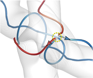
Figure 4 plots the isosurfaces of  $\phi _b=\pm 0.01$ in a subdomain
  $[{\rm \pi} /2,3{\rm \pi} /2]\times [{\rm \pi} /2,3{\rm \pi} /2]\times [{\rm \pi} /2,3{\rm \pi} /2]$ to provide a close-up view of the reconnection. We find that incipient reconnection occurs at the intersection between the MSF isosurfaces of
  $\phi _b=\pm 0.01$ and the isosurfaces of the current density magnitude
  $|\,\boldsymbol {j}|=30$, where the current sheet is shown later in figure 6 for clarity. Near this reconnection zone, we integrate two typical field lines before and after the reconnection in figures 4(a) and 4(b), respectively, which illustrates an X-type reconnection (see Priest & Forbes Reference Priest and Forbes2000; Pontin Reference Pontin2011).

Figure 4. MSF isosurfaces of  $\phi _b=\pm 0.01$ (translucent surfaces) at
  $t=1$ in the subdomain
  $[{\rm \pi} /2,3{\rm \pi} /2]\times [{\rm \pi} /2,3{\rm \pi} /2]\times [{\rm \pi} /2,3{\rm \pi} /2]$, with typical field lines (a) before and (b) after the magnetic reconnection. The reconnection zone is highlighted by the yellow dashed circle. The field lines are colour coded by
  $-1\leqslant h^*\leqslant 1$ from blue to red.
The field lines in figure 4 are colour coded by  $h^*$. Before the reconnection, two field lines within
  $\mathcal {T}_1$ and
  $\mathcal {T}_2$, respectively marked by
  $\mathcal {A}_1$ and
  $\mathcal {A}_2$ in figure 4(a), have opposite
  $h^*$ owing to their opposite chirality, and they are nearly antiparallel in the reconnection region. After the reconnection of
  $\mathcal {A}_1$ and
  $\mathcal {A}_2$, two types of field lines, marked by
  $\mathcal {A}_1'$ and
  $\mathcal {A}_2'$, form in figure 4(b). Here,
  $\mathcal {A}_1'$, a U-shaped field line encircling the central region, moves along the direction of
  $(\boldsymbol {e}_y-\boldsymbol {e}_z)$ and further reconnects in the subsequent stage;
  $\mathcal {A}_2'$, a U-shaped field line, moves along the direction of
  $(\boldsymbol {e}_z-\boldsymbol {e}_y)$ away from the plasmoid.
Figure 5 sketches the reconnection process. Two field lines  $\mathcal {A}_1$ and
  $\mathcal {A}_2$ with opposite
  $h^*$ are antiparallel in the reconnection region; then they form X-lines near magnetic null points. After the reconnection, the newly formed
  $\mathcal {A}_1'$ or
  $\mathcal {A}_2'$ consists of two pieces with opposite chirality.

Figure 5. Schematic diagram for the magnetic reconnection in figure 4. The typical field lines are colour coded by red for  $h^*>0$ and blue for
  $h^*<0$.
It is noted that this reconnection occurs symmetrically at two regions, as marked by yellow circles in figure 3(a). The reconnection regions can be roughly located by the closest antiparallel field lines between  $\mathcal {T}_1$ and
  $\mathcal {T}_2$ with the initial magnetic field. Figures 1 and 3(a) illustrate that the flux tubes facing each other merge around
  $t=1$ with negligible deformation, and the field lines within
  $-{\rm \pi} /2\leqslant \theta _1\leqslant {\rm \pi}/2$ and
  ${\rm \pi} /2\leqslant \theta _2\leqslant 3{\rm \pi} /2$ first reconnect. Considering the symmetry with
  $r_1=r_2=r$ and a large twist parameter with
  $q^2r^2\gg 1$, we approximate the cosine of the alignment angle of
  $\boldsymbol {b}_1$ and
  $\boldsymbol {b}_2$ by
 \begin{equation} \cos\theta =\dfrac{q}{\sqrt{(1+q^2r_1^2)(1+q^2r_2^2)}} (qr_1r_2\sin\theta_1\sin\theta_2+r_1\cos\theta_1\!+\!r_2\cos\theta_2) \approx\sin\theta_1\sin\theta_2. \end{equation}
The reconnection of  $\mathcal {T}_1$ and
  $\mathcal {T}_2$ implies antiparallel field lines with
  $\cos \theta \approx -1$. From (3.1), the reconnection region is close to the merged tubes in the central region with
 \begin{equation} \theta_1=3{\rm \pi}/2,\ \theta_2={\rm \pi}/2\quad \textrm{or}\quad \theta_1={\rm \pi}/2,\ \theta_2=3{\rm \pi}/2. \end{equation}
These two locations are highlighted by yellow dashed circles in figure 3(a).
Figure 6(a) plots the contour of  $|\,\boldsymbol {j}|$ on the
  $x$–
$x$– $z$ plane at
  $y=7{\rm \pi} /8$. This slice cuts through the reconnection zone, which is marked by the green dashed line in figure 3(a). We observe that a current sheet forms in between two approaching flux tubes, as highlighted by the dashed box. Therefore, the reconnection X-points can be pinpointed by the intersection between the current sheet and the region with the maximum MSF gradient. In figure 6(b), the strong Lorentz force
  $\boldsymbol {F}_L=\boldsymbol {j}\times \boldsymbol {b}$ pointing to the current sheet implies that the merger of flux tubes is driven not only by the background straining flow, but also by the induced velocity from the deformation of the flux tubes themselves. The Lorentz force can further accelerate the local velocity and generate intense local vortical structures, leading to more complex magnetic reconnections in subsequent stages.

Figure 6. Contour of  $|\,\boldsymbol {j}|$ colour coded by
  $0\leqslant |\,\boldsymbol {j}|\leqslant 30$ from blue to red on the slice
  $y=7{\rm \pi} /8$ at
  $t=1$, with MSF isolines and the projected Lorentz force (arrows). (a) The
  $x$–
$x$– $z$ slice
  $[3{\rm \pi} /4,5{\rm \pi} /4]\times [3{\rm \pi} /4,5{\rm \pi} /4]$ at
  $y=7{\rm \pi} /8$. (b) Close-up view of the region marked by the green dashed box in (a).
3.3. Stage 2: tying overhand knots
In stage 1, the helical field lines before and after the reconnection remain unknotted. Then in stage 2, some field lines in the plasmoid are tied into knots by the secondary reconnection around  $t = 1.75$. The reconnection still occurs around the intersection between MSF isosurfaces of
  $\phi _b=\pm 0.01$ and isosurfaces of
  $|\,\boldsymbol {j}|=30$. From the reconnection region, we integrate a number of field lines to seek the X-type reconnection and knotted field lines.
The close-up view of MSF isosurfaces of  $\phi _b=\pm 0.01$ at
  $t=1.75$ in figure 7 illustrates a delicate knotting process of field lines via the secondary magnetic reconnection. In figure 7(a), two typical field lines within
  $\mathcal {T}_1$ and
  $\mathcal {T}_2$, marked by
  $\mathcal {B}_1$ and
  $\mathcal {B}_2$, are almost antiparallel near the reconnection X-point before the secondary reconnection. Note that the
  $\Omega$-shaped field line
  $\mathcal {B}_1$ encircling the central region consists of two line segments with positive and negative
  $h^*$, indicating that it has undergone the first reconnection as
  $\mathcal {A}_1'$ and
  $\mathcal {A}_2'$ in figure 4(b);
  $\mathcal {B}_2$ is a helical line along the
  $y$-direction, similar to
  $\mathcal {A}_2$ in figure 4(a). The reconnection of
  $\mathcal {B}_1$ and
  $\mathcal {B}_2$ produces an overhand knot
  $\mathcal {B}_1'$ in figure 7(b). At the mean time, a U-shaped field line
  $\mathcal {B}_2'$ forms and moves along the direction of
  $(\boldsymbol {e}_z-\boldsymbol {e}_y)$ away from the central region.

Figure 7. MSF isosurfaces of  $\phi _b=\pm 0.01$ (translucent surfaces) at
  $t=1.75$ in the subdomain
  $[{\rm \pi} /2,3{\rm \pi} /2]\times [{\rm \pi} /2,3{\rm \pi} /2]\times [{\rm \pi} /2,3{\rm \pi} /2]$, with typical field lines (a) before and (b) after the magnetic reconnection. The reconnection zone is highlighted by the yellow dashed circle. The field lines are colour coded by
  $-1\leqslant h^*\leqslant 1$ from blue to red.
Figure 8 sketches the formation of the overhand knot via the secondary reconnection. It is interesting that the knotting process is via such a simple antiparallel reconnection in the present case, rather than more complex mechanisms such as bridging and threading in vortex reconnection (e.g. Melander & Hussain Reference Melander and Hussain1988; Kida & Takaoka Reference Kida and Takaoka1994; Yao & Hussain Reference Yao and Hussain2020). After this reconnection,  $\mathcal {B}_1'$ consists of three pieces. The piece with positive
  $h^*$ is embedded into the other two with negative
  $h^*$. Thus, this topological change also makes the geometry of field lines more complex.

Figure 8. Schematic diagram for tying the overhand knot via the magnetic reconnection in figure 7. The typical field lines are colour coded by red for  $h^*>0$ and blue for
  $h^*<0$.
The reconnection location at  $t=1.75$ is similar to that at
  $t=1$. Figure 9 plots the contour of
  $|\,\boldsymbol {j}|$ on the slice at
  $y=7{\rm \pi} /8$. Driven by the combination of the fluid velocity and the velocity induced by the Lorentz force, two MSF isosurfaces of
  $\phi _b=\pm 0.001$ collide at the reconnection point, along with the formation of the current sheet in between the two approaching flux tubes.

Figure 9. Contour of  $|\,\boldsymbol {j}|$ colour coded by
  $0\leqslant |\,\boldsymbol {j}|\leqslant 30$ from blue to red on the slice
  $y=7{\rm \pi} /8$ at
  $t=1.75$, with MSF isolines and the projected Lorentz force (arrows). (a) The
  $x$–
$x$– $z$ slice
  $[3{\rm \pi} /4,5{\rm \pi} /4]\times [3{\rm \pi} /4,5{\rm \pi} /4]$ at
  $y=7{\rm \pi} /8$. (b) Close-up view of the region marked by the green dashed box in (a).
The knotting process can happen at a range of  $\phi _b$. Since the MSF isosurfaces of different isocontour levels are coaxial tubes, we can distinguish inner and outer flux tubes by setting particular thresholds of
  $\phi _b$, and quantify their respective influences on the statistics and important events in the flow evolution. Considering the inner tubes within
  $\varOmega _{I}=\{\boldsymbol {x}\in \mathbb {R}^3\,|\,0.5<\phi _b(\boldsymbol {x})\leqslant 1\}$ and outer tubes within
  $\varOmega _{O}=\{\boldsymbol {x}\in \mathbb {R}^3\,|\,0.1<\phi _b(\boldsymbol {x})\leqslant 0.5\}$, the temporal evolution of the volume-averaged kinetic energy and normalized magnetic helicity density for the inner and outer flux tubes is shown in figure 10.

Figure 10. Temporal evolution of volume-averaged (a) kinetic energy and (b) normalized magnetic helicity within inner or outer flux tubes.
At early times, both  $\langle E_u \rangle _I$ and
  $\langle E_u \rangle _O$ decay due to the viscous dissipation in figure 10(a), where
  $\langle \cdot \rangle _I$ and
  $\langle \cdot \rangle _O$ denote the volume averages over
  $\varOmega _I$ and
  $\varOmega _O$, respectively. Around
  $t\approx 1$,
  $\langle E_u \rangle _I$ and
  $\langle E_u \rangle _O$ begin to rise with time, consistent with the incipient reconnection time
  $t=1$. Then the primary peaks of
  $\langle E_u \rangle _I$ and
  $\langle E_u \rangle _O$ occur at
  $1<t<2$. These volume averages effectively avoid the interference from the background flow outside the tube, i.e. in the region with
  $-0.1\leqslant \phi _b\leqslant 0.1$, on the flow statistics. The peak of
  $\langle E_u \rangle _I$ is higher than that of
  $\langle E_u \rangle _O$. This implies that the energy conversion from
  $E_b$ to
  $E_u$ within inner tubes is stronger than that within outer tubes through more frequent magnetic reconnections and stronger release of the magnetic energy.
The exact quantification of the helicity evolution is difficult in the present configuration owing to the periodic boundary condition with net fluxes (e.g. Berger Reference Berger1997) and the vanishing total helicity over the entire domain. As possible measures of knottedness or helical degree of field lines,  $\langle h^* \rangle _I$ and
  $\langle h^* \rangle _O$ surge around
  $t=1.5$ in figure 10(b), and
  $\langle h^* \rangle _I$ peaks at
  $t=2$, consistent with the knotting of field lines in figure 7. We remark that the helicities
  $\langle h \rangle _I$ and
  $\langle h \rangle _O$ of inner and outer tubes generally decay with time due to the dissipation, so they cannot distinguish the knotting period and are omitted here. Moreover, the volume-averaged helicity density over the complement region
  $\{\boldsymbol {x}\in \mathbb {R}^3\,|\,0<\phi _b\leqslant 0.1\}$ is negligible.
Based on the MSF, the reconnection and tying of field lines can be characterized by the magnetic flux  $F\equiv \int _{\mathcal {S}}\boldsymbol {b}\boldsymbol {\cdot }\boldsymbol {n}\, \mathrm {d}\mathcal {S}$ through a symmetric plane with the surface normal
  $\boldsymbol {n}$. Considering the flow symmetries, two typical magnetic fluxes
 \begin{equation} \left.\begin{gathered} F_1=\frac{1}{\sqrt{2}}\int_{\mathcal{S}_1}(b_z(\boldsymbol{x})- b_y(\boldsymbol{x}))\,\mathrm{d}\mathcal{S},\\ F_2=\frac{1}{\sqrt{2}}\int_{\mathcal{S}_2}(b_z(\boldsymbol{x})+ b_y(\boldsymbol{x}))\,\mathrm{d}\mathcal{S} \end{gathered}\right\} \end{equation}
of  $\mathcal {T}_1$ through diagonal planes are calculated, where
  $\mathcal {S}_1$ denotes the region enclosed by
  $\phi _b=0$ and
  $\phi _b=1$ on the plane of
  $y+z=2{\rm \pi}$, and
  $\mathcal {S}_2$ denotes the region enclosed by
  $\phi _b=0$ and
  $\phi _b=1$ on the plane of
  $y-z=0$. We remark that the poloidal/toroidal flux (see Moffatt & Ricca Reference Moffatt and Ricca1992) is not calculated here, because it is difficult to accurately determine the centreline of the very distorted flux tubes during and after reconnection.
The temporal evolutions of  $F_1$ and
  $F_2$ are shown in figure 11. The initial magnetic field in (2.6) and (2.10) of
  $\mathcal {T}_1$ implies
  $F_1(t=0)=F_2(t=0)=-\varGamma /\sqrt {2}$. We observe that both fluxes are nearly conserved before the first reconnection at
  $t=1$, consistent with the Alfvén theorem. Around
  $t=1$, the magnitude of the fluxes significantly decays owing to the direction change of field lines during the reconnection (see figure 4).

Figure 11. Magnetic fluxes (3.3) through diagonal symmetric planes.
Figure 12 plots contours of the flux density  $(b_z-b_y)/\sqrt {2}$ of
  $F_1$ on the diagonal symmetric plane
  $y+z=2{\rm \pi}$ in the subdomain
  $[3{\rm \pi} /4,5{\rm \pi} /4]\times [3{\rm \pi} /4,5{\rm \pi} /4]\times [3{\rm \pi} /4,5{\rm \pi} /4]$ with some typical field lines from two perspective views. The boundary of
  $\mathcal {T}_1$, the isosurface of
  $\phi _b=0.01$, is marked by the thick line on the plane. At
  $t=1$, the field lines integrated on the outer side of the central region in figure 12(a) only have slight deformation compared to the initial configuration. On the other hand, the directions of the field lines integrated on the inner side of the central region have significant changes in figure 12(b). Owing to the reconnection, some of these field lines of
  $\mathcal {T}_1$ originally through
  $\mathcal {S}_1$ no longer pass through
  $\mathcal {S}_1$, and the angles between the field lines and the symmetric plane are decreased. Hence, the strength of
  $F_1$ is weakened in figure 11 at
  $t=1$.

Figure 12. Contours of the flux density of  $F_1$ on the diagonal symmetric plane
  $y+z=2{\rm \pi}$ from two perspectives at (a,b)
  $t=1$ and (c,d)
  $t=1.75$ in the subdomain
  $[3{\rm \pi} /4,5{\rm \pi} /4]\times [3{\rm \pi} /4,5{\rm \pi} /4]\times [3{\rm \pi} /4,5{\rm \pi} /4]$, where the arrow denotes the normal
  $\boldsymbol {n}$ of the symmetric plane. Some field lines are integrated on the MSF isosurface of
  $\phi _b=\pm 0.01$ (translucent surface). Region
  $\mathcal {S}_1$ is enclosed by the intersection (yellow line) of the MSF isosurface and the diagonal plane.
From  $t=1.5$ to
  $t=2$, the profile of
  $F_1$ shows a plateau in figure 11, signalling the secondary reconnection of field lines. At
  $t=1.75$, magnetic overhand knots are generated after the reconnection. The released kinetic energy shown in figure 2(a) accelerates the distortion of the field lines in the central region, and produces more positive flux with larger angle between field lines and the plane in figure 12(c). Meanwhile, the angle between field lines and the plane also increases in the central region, producing more negative flux in figure 12(d). Owing to the two competing effects, flux
  $F_1$ through
  $\mathcal {S}_1$ remains almost unchanged from
  $t=1.5$ to
  $t=2$.
3.4. Stage 3: cascade of tying complex knots
After the formation of overhand knots in the plasmoid, a sequence of reconnection events at the same regions as marked in figure 3(a) leads to a cascade of tying more complex knots. Figure 13 illustrates the formation of double overhand knots at  $t=2$. Two typical field lines within
  $\mathcal {T}_1$ and
  $\mathcal {T}_2$ are marked by
  $\mathcal {C}_1$ and
  $\mathcal {C}_2$ before the tertiary reconnection. Here,
  $\mathcal {C}_1$ is an unknotted line encircling the plasmoid, and has highly convoluted geometry colour coded by
  $h^*$ with alternating signs;
  $\mathcal {C}_2$ is a helical line along the
  $y$-direction, with geometry similar to
  $\mathcal {A}_2$ and
  $\mathcal {B}_2$. The reconnection of
  $\mathcal {C}_1$ and
  $\mathcal {C}_2$ forms a double overhand knot
  $\mathcal {C}_1'$ along the
  $y$-direction and a U-shaped line
  $\mathcal {C}_2'$ moving away from the reconnection zone. We find that the positions of the three reconnections in figures 4, 7 and 13 are very close to the theoretical estimation in (3.2a,b). In addition, the initial magnetic condition has an impact on the knotting process, which is discussed in appendix B.

Figure 13. MSF isosurfaces of  $\phi _b=\pm 0.01$ (translucent surfaces) at
  $t=2$ in the subdomain
  $[{\rm \pi} /2,3{\rm \pi} /2]\times [{\rm \pi} /2,3{\rm \pi} /2]\times [{\rm \pi} /2,3{\rm \pi} /2]$, with typical field lines (a) before and (b) after the magnetic reconnection. The reconnection zone is highlighted by the yellow dashed circle. The field lines are colour coded by
  $-1\leqslant h^*\leqslant 1$ from blue to red.
The observations in figures 4, 7 and 13 imply that the major mechanism for the current magnetic reconnection is the X-type reconnection (see Priest & Forbes Reference Priest and Forbes2000; Pontin Reference Pontin2011), which is similar to viscous cancellation rather than bridging (see Melander & Hussain Reference Melander and Hussain1988; Kida & Takaoka Reference Kida and Takaoka1994) in vortex reconnection. It is noted that vortex lines can be tangled under the strong self-induced local velocity generated in the incipient reconnection of vortex lines, whereas the reconnection of field lines can only alter the local velocity via an implicit way at moderate and large interaction parameters (see Kivotides Reference Kivotides2018).
The influence of the magnetic knot cascade on the local flow motion is through the Lorentz force. figure 14 shows the knot motion projected onto the  $y$–
$y$– $z$ plane, along with the isoline of
  $\phi _b=0.01$ and the projected velocity field on the slice at
  $x=7{\rm \pi} /8$. Several knotted field lines are integrated from the reconnection regions. We observe that, in general, the local velocity is enhanced and small-scale vortical structures are generated during the magnetic reconnection. In figure 14(a), the velocity shows a vortex pattern, making the knots rotate around the
  $x$-axis and distort at
  $t=1.75$. In figure 14(b), the velocity components inclined to the
  $z$-direction gradually dominate. They drive the U-shaped field lines after the reconnection to separate, and stretch the knots along the
  $z$-direction. The knotting process is gradually spread from inner tubes to outer tubes, causing the growth of
  $\langle E_u \rangle _O$ and
  $\langle h^*_m \rangle _O$ in figure 10 around
  $t=1.75$. In figure 14(c), the knots move closer to the reconnection zone, triggering further reconnections to generate triple overhand knots and more complex knots at
  $t=2.25$. Furthermore, induced by the Lorentz force term in (2.3), the initially closed, unknotted vortex lines also become highly tangled and twisted, and some of them can be knotted (not shown), which is worth investigating in future work.

Figure 14. The projected velocity (arrows) on the  $y$–
$y$– $z$ slice
  $[3{\rm \pi} /4,5{\rm \pi} /4]\times [3{\rm \pi} /4,5{\rm \pi} /4]$ at
  $x=7{\rm \pi} /8$, along with a set of knotted field lines integrated from the reconnection regions and the isoline of
  $\phi _b=0.01$: (a)
  $t=1.75$, (b)
  $t=2$ and (c)
  $t=2.25$.
We use the minimal crossing number, which is a knot invariant under Reidemeister moves (Reidemeister Reference Reidemeister1927; Alexander & Briggs Reference Alexander and Briggs1926), to quantify the knotting cascade via a sequence of magnetic reconnections. The typical knotted field lines in the plasmoid, shown in figures 4, 7 and 13, are projected from proper perspective views to depict a ‘knot diagram’ in figure 15(a–c). Reducible or nugatory crossings (Hoste, Thistlethwaite & Weeks Reference Hoste, Thistlethwaite and Weeks1998) can be removed in knot diagrams by proper Reidemeister moves. Meanwhile, non-reducible crossings, counted by the minimal crossing number  $n_c$ in reduced knot diagrams, are marked by thick ‘
 $-$’ in figure 15(a–c). We find that
  $n_c$ grows with time, indicating the increasing complexity of knots in a cascade process.

Figure 15. (a–c) Cascade of tying magnetic knots in the plasmoid, with non-reducible crossings marked by thick ‘ $-$’: (a) overhand knot (trefoil knot) at
  $t=1.75$, (b) double overhand knot (cinquefoil knot) at
  $t=2.0$, and (c) triple overhand knot (septafoil knot) at
  $t=2.25$. (d–f) Corresponding reduced knot diagrams of torus knots (these knots are equivalent to those in the upper row): (d) trefoil knot, (e) cinquefoil knot, and (f) septafoil knot.
If the ends of the field lines at the boundary of  $\varOmega$, e.g. points
  $\mathcal {P}_1$ and
  $\mathcal {P}_2$ of the overhand knot in figure 15(a), are closed at infinity without intersecting other field lines in
  $\varOmega$, the knots are equivalent to the torus knots, e.g. the trefoil knot with
  $n_c=3$ in figures 15(d). For more complex knots, we demonstrate how to deform the double overhand knot in figure 15(b) into the cinquefoil knot in figure 15(e) using Reidemeister moves. First, the two ends
  $\mathcal {P}_1$ and
  $\mathcal {P}_2$ of the field line are connected to form a loop. Second, part
  $\mathcal {L}_1$ marked by the red solid curve is moved completely over crossing
  ${O}_0$, from right to left as marked by the red arrow, by the type-III Reidemeister move, and part
  $\mathcal {L}_2$ marked by the blue dashed line is moved under crossing
  ${O}_0$ from left to right by the type-III Reidemeister move. Finally,
  $\mathcal {L}_1$ is moved over crossing
  ${O}_1$ and
  $\mathcal {L}_2$ is moved under crossing
  ${O}_2$ by type-III Reidemeister moves. Thus, the crossing number of the two knots in a minimal two-dimensional knot diagram is
  $n_c=5$. Similarly, the triple overhand knot in figure 15(c) is equivalent to the septafoil knot with
  $n_c=7$ in figure 15(f) after proper Reidemeister moves.
Figure 16 plots a highly coiled field line (blue) at  $t=2.25$, surrounded by the triple overhand knot (red) shown in figure 15(c). The inner field line, in the global shape of a Mobius band, has thousands of turns around the plasmoid. The stretching effect shown in figure 14(b,c) appears to suppress the knotting process by merging neighbouring field lines, and both
  $\langle h^* \rangle _I$ and
  $\langle h^* \rangle _O$ begin to decay around
  $t=2.25$. In addition, we did not observe any clear sign of the relaxation of magnetic knots (e.g. Taylor Reference Taylor1974; Moffatt Reference Moffatt1990) as in Xiong & Yang (Reference Xiong and Yang2020). A possible reason is that each knotted field line in the present study is not isolated and it is distorted by fluctuating local fluid motion.

Figure 16. Complex knots in the plasmoid at  $t=2.25$. (a) MSF isosurfaces of
  $\phi _b=\pm 0.01$ (translucent surfaces) with typical field lines. (b) Close-up view of a triple overhand knot (red) and a highly coiled field line (blue).
The knot cascade slows down and then terminates at later times owing to the separation of the U-shaped tubes shown in figure 3(c,d). The plasmoid at the centre is stretched along the direction of  $(\boldsymbol {e}_z-\boldsymbol {e}_y)$. The highly coiled field lines are severed by successive reconnections with the cancellation of opposite directions of the field lines near the centre of
  $\varOmega$. Finally, the untied magnetic knots gradually vanish in the central region at
  $t>4$ with resistive and viscous dissipations, which is similar to the observation in Linton et al. (Reference Linton, Dahlburg and Antiochos2001).
3.5. Quantification of the magnetic knot cascade
We have demonstrated a knot cascade of field lines through a sequence of reconnection events in the evolution of helical flux tubes. Starting from the unknotted state, the first overhand knot with  $n_c=3$ forms around
  $t=1.75$, and then
  $n_c$ is incremented by two in each subsequent reconnection event at the same region near (3.2a,b) in the plasmoid until the separation of the U-shaped tubes and the vanishing of the plasmoid at late times.
In order to further quantify the knot cascade using the statistical distribution of knot types, we integrate 3700 field lines in both forward and backward directions from spatially uniform points sampled on the symmetric plane
 \begin{equation} \mathcal{S}^*=\left\{\boldsymbol{x} \,\Bigg|\,|\phi_b(\boldsymbol{x})|\geqslant0.1, \frac{3{\rm \pi}}{4}\leqslant x\leqslant \frac{5{\rm \pi}}{4},y={\rm \pi},{\rm \pi}\leqslant z\leqslant \frac{5{\rm \pi}}{4} \right\} \end{equation}
within the plasmoid at each of the three typical times  $t=1.75$, 2 and 2.25. Each field line is extracted as a set of discretized points in three dimensions; then we artificially add an unknotted and unlinked line segment consisting of several ghost points outside
  $\varOmega$ to close the two ends of a field line to form a loop.
The knot type of the closed field lines, in terms of the Alexander–Briggs notation (Alexander & Briggs Reference Alexander and Briggs1926), is identified by a knot analysis toolkit ‘pyknotid’ (Taylor et al. Reference Taylor2017). In this toolkit, the Alexander polynomial is calculated via a standard matrix determinant algorithm (see Orlandini & Whittington Reference Orlandini and Whittington2007). Although the Alexander polynomial has some weaknesses to distinguish complex knots (see Kauffman Reference Kauffman2001; Liu & Ricca Reference Liu and Ricca2015), it is sufficient to identify simple torus knots (e.g. Kuei et al. Reference Kuei, Słowicka, Ekiel-Jeżewska, Wajnryb and Stone2015; Mesgarnezhad et al. Reference Mesgarnezhad, Cooper, Baggaley and Barenghi2017) in the present study.
The probability density function (p.d.f.) of the identified knot type at the three typical times is plotted in figure 17. Here, the p.d.f. of unknotted field lines is omitted for clarity. Additionally,  $12.5\,\%$ of extracted field lines at
  $t=2.25$ are highly convoluted in the plasmoid as observed in figure 16. Their knot types, which have large crossing numbers or are not torus knots, may not be accurately identified owing to the finite spatial resolution and total integration steps for extracting the field lines, so the p.d.f.s for these field lines are also omitted.

Figure 17. The p.d.f. of magnetic knot types in terms of the Alexander–Briggs notation at  $t=1.75$,
  $t=2$ and
  $t=2.25$.
The knot statistics in figure 17 reveals that the ratio of knotted field lines to all the field lines in the central region surges with time, e.g. less than  $4\,\%$ of field lines are knotted at
  $t=1.75$, and this ratio grows to
  $20\,\%$ at
  $t=2.25$. As illustrated in figure 15, the p.d.f. peak migrates from trefoil knots
  $3_1$ at
  $t=1.75$, through cinquefoil knots
  $5_1$ at
  $t=2$, to septafoil knots
  $7_1$ at
  $t=2.25$. Moreover, the p.d.f. is broadened with time, indicating that there are various types of complex knots at late times.
It is interesting that the knotting cascade of field lines in MHD flows is in contrast with the unknotting cascade of knotted vortex filaments found in HD flows (Kleckner & Irvine Reference Kleckner and Irvine2013; Xiong & Yang Reference Xiong and Yang2019a) and superfluids (Kleckner et al. Reference Kleckner, Kauffman and Irvine2016). The possible reason is that the field lines tend to be twisted by the Lorentz force. The resultant helical field lines have higher probabilities than straight lines to be tied into knots via the magnetic reconnection in MHD flows, as illustrated in figure 7. By contrast, the twist of vortex lines can decay rapidly without external forcing in HD flows (see Scheeler et al. Reference Scheeler, van Rees, Kedia, Kleckner and Irvine2017; Xiong & Yang Reference Xiong and Yang2020), so that vortex lines appear to have lower probabilities to be knotted than magnetic field lines.
In the characterization of the knotting cascade, the MSF plays an important role to determine the reconnection region and the starting points for integrating knotted field lines. On the other hand, there are several issues to hinder further quantifications of the knotting cascade in dissipative systems using topological diagnostic tools such as adapted knot polynomials (see Liu & Ricca Reference Liu and Ricca2015, Reference Liu and Ricca2016) and the pathway analysis in terms of the minimal crossing number and topological writhe (see Kleckner et al. Reference Kleckner, Kauffman and Irvine2016).
First, it is hard, or even not well defined in principle, to track a particular field line in a resistive MHD flow (see Hao et al. Reference Hao, Xiong and Yang2019). Second, there is a lack of a general algorithm to compute knot polynomials for complex knots in a periodic domain (see Liu & Ricca Reference Liu and Ricca2015; Cooper et al. Reference Cooper, Mesgarnezhad, Baggaley and Barenghi2019). Third, there are an infinite number of field/vortex lines in complex MHD/HD flows, so it is not clear how to characterize the influence of the knotting/unknotting cascade on important flow statistics. Therefore, the full topological diagram and the significance of knotting/unknotting cascade in MHD/HD turbulence remains an open problem.
4. Conclusions
We report the knot cascade of magnetic field lines via the stepwise reconnection of a pair of mutually perpendicular helical flux tubes with opposite helicities and  $q=\pm 10$. The MSF method is used to visualize the morphology of flux tubes with attached field lines and to locate the reconnection regions with theoretical analysis. Based on the MSF visualization, the evolution of the flux tubes is divided into three stages. Incipient magnetic reconnection occurs around
  $t=1$ at the locations marked in figure 3(a). This X-type reconnection generates antiparallel U-shaped field lines moving in opposite directions away from the plasmoid, and is quantified by the decay of magnetic flux through the region enclosed by MSF isolines on the diagonal symmetric planes.
Secondary reconnection occurs around  $t=1.75$ near the same location as the first reconnection. This reconnection of a U-shaped helical line encircling the central region and a helical line along a straight tube ties an overhand magnetic knot. The knotting process coincides with the rise of the kinetic energy and the normalized helicity density averaged over inner flux tubes with
  $0.1<\phi _b\leqslant 0.5$, indicating a strong release of magnetic energy during the reconnection.
The distorted flux tubes generate the Lorentz force to induce a vortical-like velocity field in the plasmoid. Under this local motion, the knotted field lines are rotated and stretched. This nonlinear evolution triggers the tertiary reconnection to form double overhand knots around  $t=2$ and further reconnections to produce triple overhand knots and more complex knots around
  $t=2.25$.
The minimum crossing numbers  $n_c = 3$ at
  $t=1.75$,
  $n_c = 5$ at
  $t=2$ and
  $n_c = 5$ at
  $t=2.25$ of these knots are obtained from extracted typical field lines integrated from the reconnection region with Reidemeister moves. The statistical progression from unknotted field lines, through simple knots, to complex knots is further quantified by the migrating and broadening p.d.f. of knot types with time. Thus, we demonstrate a knotting cascade of field lines through a sequence of reconnection events and its influence on the magnetic energy release in a finite time period. Finally, the knot cascade slows down and then terminates in the dissipative MHD flow.
In future work, the knotting/unknotting cascade and its significance on flow dynamics are expected to be investigated in MHD/HD turbulence. More advanced methods need to be developed to identify frequent reconnection events and to distinguish complex knots. Furthermore, the parameters  $Re$,
$Re$,  $Re_m$ and
  $N_i$ are relatively moderate in the present study, and we expect more complex dynamics of field lines for larger parameters, e.g. more tangled field lines during reconnection (e.g. Yao & Hussain Reference Yao and Hussain2020) and stronger interactions between magnetic and vorticity fields via the Lorentz force (e.g. Kivotides Reference Kivotides2018).
Acknowledgements
The authors thank S. Xiong, W. Shen and X. Liu for helpful comments. Numerical simulations were carried out on the TH-2A supercomputer in Guangzhou, China.
Funding
This work has been supported in part by the National Natural Science Foundation of China (grant nos 11925201, 11988102, 91952108 and 91841302).
Declaration of interests
The authors report no conflict of interest.
Appendix A. Identification methods of flux tubes
The flux tubes are usually visualized by the isosurface of the magnetic strength  $|\boldsymbol {b}|$ (e.g. Linton et al. Reference Linton, Dahlburg and Antiochos2001) or bundles of field lines (e.g. Dahlburg, Antiochos & Norton Reference Dahlburg, Antiochos and Norton1997; Hesse, Forbes & Birn Reference Hesse, Forbes and Birn2005) in existing studies. These methods are simple to implement but have weaknesses for tracking coherent flux tubes in time (see Lau & Finn Reference Lau and Finn1996), such as the lack of time coherence and the ad hoc choice of isocontour level at different times, which are similar to the issues for identifying vortex tubes (see Xiong & Yang Reference Xiong and Yang2019b).
Figure 18 plots the averaged MSF deviations (2.18) in terms of the MSF solution and the magnetic strength. We find that  $\langle |\lambda _b| \rangle$ for
  $\phi =\phi _b$ is less than
  $1\,\%$, which is very low and consistent with the accurate identification of flux tubes in figure 3. By contrast,
  $\langle |\lambda _b| \rangle$ for
  $\phi =|\boldsymbol {b}|$ is around
  $10\,\%$ at
  $t=2$ and
  $20\,\%$ at
  $t=4$. figure 19 plots the isosurfaces of
  $|\boldsymbol {b}|$ and some field lines integrated on the surfaces at
  $t=2$ and
  $t=4$. We observe that the field lines notably deviate from the surfaces, corresponding to the large MSF deviation in figure 18. Therefore, compared with the regular visualization of
  $|\boldsymbol {b}|$, the Lagrangian-based MSF method facilitates the identification of flux tubes in a temporal evolution and provides accurate integral boundaries for calculating the magnetic fluxes in figure 11.

Figure 18. Temporal evolution of MSF deviations for the MSF solution and the magnetic magnitude.

Figure 19. Isosurfaces of  $|\boldsymbol {b}|=0.5|\boldsymbol {b}|_{{max}}$ at (a)
  $t=2$ and (b)
  $t=4$, where
  $|\boldsymbol {b}|_{{max}}$ denotes the maximum
  $|\boldsymbol {b}|$ in
  $\varOmega$. Some field lines are integrated on the surfaces.
In addition, if we evolve  $\phi _b$ as a pure Lagrangian scalar by solving
  $\partial \phi _b/\partial t + \boldsymbol {u}\boldsymbol {\cdot } \boldsymbol {\nabla } \phi _b =0$, in the same form as the prediction substep in (2.16), the isosurface of
  $\phi _b$ is a material surface. We find that the evolutionary geometry of the material surface with the maximum
  $\langle |\lambda _b| \rangle \approx 5\,\%$ is similar to that of the MSF isosurface. This indicates that the MSF visualization has an essential Lagrangian nature, and the two-time method effectively reduces the MSF deviation owing to breakdown of the Alfvén theorem in the ordinary Lagrangian surface tracking via the correction substep in (2.17).
Appendix B. Effects of the initial condition on knotting process
The initial condition of the magnetic field can have an impact on the knotting process of helical field lines. First, to demonstrate the effects of the initial twist, we perform two additional simulations with  $q=5$ and
  $q=15$ for
  $\mathcal {T}_1$, where the corresponding negative
  $q$ values for
  $\mathcal {T}_2$ are omitted for clarity. The other DNS set-ups for the two cases are the same as those of
  $q=10$. Additionally, if initial helical tubes have the same chirality, e.g.
  $q=10$ for both
  $\mathcal {T}_1$ and
  $\mathcal {T}_2$, their evolution has the ‘tunnel interaction’ (see Linton et al. Reference Linton, Dahlburg and Antiochos2001) without knot cascade.
For various  $q$, figure 20 compares temporal evolutions of the volume-averaged kinetic energy and normalized magnetic helicity density within inner flux tubes. All the profiles are normalized by their initial values. For all three cases,
  $\langle E_u \rangle _I/\langle E_u \rangle _{I0}$ first decays and then rises. The incipient rising time is advanced with the increase of
  $q$, indicating that the energy conversion accelerates with
  $q$. In figure 20(b), the peak of
  $\langle h^* \rangle _I/\langle h^* \rangle _{I0}$ with
  $q=15$ occurs earlier and the peak value is higher than those in the case with
  $q=10$. For the case with
  $q=5$,
  $\langle h^* \rangle _I/\langle h^* \rangle _{I0}$ monotonically decays without peaks.

Figure 20. Temporal evolution of the volume-averaged (a) kinetic energy and (b) normalized magnetic helicity within inner flux tubes in the DNS cases with various  $q$.
$q$.
Figure 21 plots MSF isosurfaces of  $\phi _v=\pm 0.01$ with
  $q=5$ and
  $q=15$ at
  $t=1.75$ and some typical field lines integrated on the surfaces. The distortion degree of the flux tubes and field lines grows with
  $q$. For
  $q=5$, the deformation of flux tubes is small and the geometry of field lines is simple. Some U-shaped field lines form after the reconnection with a low rate and they remain unknotted, consistent with the relatively steady profiles of the kinetic energy and normalized helicity density within inner flux tubes in figure 20. By contrast, for
  $q=15$, knotted and highly coiled field lines are generated via reconnections in the plasmoid. We plot a typical double overhand knot and a highly coiled field line with many turns around the plasmoid in figure 21(d). Their occurrence time
  $t=1.75$ is earlier than that for the case with
  $q=10$ shown in figures 7 and 16. Hence, the increase of
  $q$ accelerates the reconnection and tying processes of field lines and enhances the energy conversion, consistent with the strongest peaks of
  $\langle E_u \rangle _I/\langle E_u \rangle _{I0}$ and
  $\langle h^* \rangle _I/\langle h^* \rangle _{I0}$ for
  $q=15$ in figure 20.

Figure 21. Isosurfaces of  $\phi _b=\pm 0.01$ for cases with (a)
  $q=5$ and (b)
  $q=15$ at
  $t=1.75$. Some field lines are integrated and plotted on the isosurfaces colour coded by
  $-1\leqslant h^*\leqslant 1$ from blue to red. Close-up views in the plasmoid for cases with (c)
  $q=5$ and (d)
  $q=15$ at
  $t=1.75$, with some field lines colour coded by
  $-1\leqslant h^*\leqslant 1$ from blue to red.
Second, we investigate effects of the initial magnetic distribution on the knotting process of helical field lines by performing two additional simulations with different initial magnetic profiles  $f_1(r) = \,f_0(r)$ in (2.8) with a smaller
  $K=0.5$ and
 \begin{equation} f_2(r)= \begin{cases} b_0 [1-g(r/r_c) ], & r\leqslant r_c, \\ 0, & r>r_c, \end{cases} \end{equation}
with  $K=10$. figure 22 shows that
  $f_1(r)<\,f_0(r)<\,f_2(r)$ for
  $0<r<r_c$, causing the largest initial circumferential component
  $b_\theta = qrf(r)$ for
  $f_2$ and the smallest
  $b_\theta$ for
  $f_1$.

Figure 22. Comparison of different initial magnetic distributions of (a) the axial component and (b) the circumferential component.
Since the knotting process is triggered by the antiparallel reconnection of helical field lines, as shown in figures 7 and 8 and implied by the  $q$ effect in figure 21, the strong initial
  $b_\theta$ at large
  $r$ in figure 22(b) can accelerate the reconnection and the knotting cascade starting from the peripheral region of helical flux tubes. For the case with initial magnetic distribution
  $f_2$, figure 23 illustrates that the formation time of overhand knots is around
  $t=0.75$, which is much earlier than
  $t=1.75$ for initial
  $f_0$, and the subsequent cascade towards
  $5_1$,
  $7_1$ and more complex knots from
  $t=0.75$ to
  $t=1.25$ is faster than that from
  $t=1.75$ to
  $t=2.25$ for initial
  $f_0$. Identified from the field lines sampled through
  $\mathcal {S}^*$ in (3.4), we calculate that
  $1.5\,\%$ and
  $47.2\,\%$ of sampled field lines are knotted at
  $t=0.75$ and
  $t=1.25$, respectively. In contrast, there is no knotting in the case with initial
  $f_1$, and the evolutionary geometry of the isosurface of
  $\phi _b$ is very similar to that in figure 21(a,c).

Figure 23. Cascade of tying magnetic knots in the plasmoid in the case with initial  $f_2$, which is visualized by typical field lines: (a) overhand knot (trefoil knot) at
  $t=0.75$, (b) double overhand knot (cinquefoil knot) at
  $t=1.0$, and (c) triple overhand knot (septafoil knot) at
  $t=1.25$.
Another factor to influence the knotting process of field lines is the interaction parameter. Compared to the base DNS case with  $b_0 = 3.068$ in (2.8), we perform two additional cases for a smaller
  $N_i = 2.26\times 10^{-1}$ with
  $b_0=0.01\times 3.068$ and a larger
  $N_i = 5.65\times 10^{4}$ with
  $b_0=5\times 3.068$. Under the weak action of magnetic field on the velocity field with
  $N_i = 2.26\times 10^{-1}$, the magnetic surface is similar to the material surface (see Kivotides Reference Kivotides2018). Two flux tubes are flattened in the central region without knotting process, similar to the observation in figure 21(a,c). Under the very strong action of the magnetic field with
  $N_i = 5.65\times 10^{4}$, the morphology of the MSF isosurface is similar to that in figure 21(b). The knotting process begins around
  $t=0.75$, and then
  $31.1\,\%$ of field lines sampled through
  $\mathcal {S}^*$ are knotted at
  $t=1.25$. Thus, the helical degree of field lines tends to be maintained towards the force-free state (Woltjer Reference Woltjer1958) and the knotting process is accelerated at large interaction parameters.


