


1. INTRODUCTION
Feature technology is considered an essential tool for integrating design and manufacturing (Gupta et al., Reference Gupta, Regli and Nau1994; Dong et al., Reference Dong, Parsaei and Leep1996; Amaitik & Kiliç, Reference Amaitik and Kiliç2004; Tolouei-Rad Reference Tolouei-Rad2006). Feature recognition maps a geometric model to application-specific feature models using various recognition rule sets regarding the application. Feature recognition techniques are required in all systems that use features for analysis and decision making. Various feature recognition methods have been developed such as syntactic pattern recognition, state transition diagrams, logic rules, graph-based approach, volumetric decomposition, hint-based approach, and hybrid approaches (Babić et al., Reference Babić, Nešić and Miljković2008). However, there are still problems with feature recognition that hinder its practical applications, such as inability to learn, limited range of recognition, and low speed. Artificial neural network (ANN)-based feature recognition techniques have become attractive because they can eliminate some drawbacks of conventional feature recognition (Ding & Yue, Reference Ding and Yue2004).
Feature represents one of the most important notions in theoretical and industrial concepts related to computer-aided activities in the product life cycle. Feature is probably the most often and most diversely defined notion in the field of production engineering. These definitions differ in dependence as to whether they have a general or particular character. They have evolved in time following development of scientific trends. In the first appendix of his doctoral thesis, Salomons (Reference Salomons1995) gave an exceptional review of feature definitions and the current state of the art, as well as the application of technologies based on it. However, even today, the academic or research community has not been able to find a universal and globally acceptable definition of this notion nor reach a consensus in connection with accompanying terminology.
In this paper the authors will lobby for a newer definition of feature given by Patrick Martin (Reference Martin, Bramley, Brissaud, Coutellier and McMahon2005): “A feature is a semantic group (modeling atom), characterized by a set of parameters, used to describe an object which cannot be broken down, used in reasoning relative to one or more activities linked to the design and use of products and production systems.”
The purpose of modeling using features is to formalize expert accomplishments, make knowledge capitalization easier, provide data on all production activities in early design phases, and advance communication between people cooperating on product creation in all phases of its life cycle.
The term feature has a universal character. When a special application aspect needs to be emphasized, this is done using a domain-specific attribute (geometrical features, manufacturing features, functional features, metrological features, etc.). Concerning manufacturing features in this paper, the authors have sometimes omitted the attribute manufacturing in situations when no confusion on what type of feature is in question.
The design concept based on features is characterized by a high semantic level, but it still cannot support every possible industrial context in a general formulation. This is where the significance of mapping features from one to another application domain is noted. For the problems dealt with in this work, the mapping process from a geometrical (functional) domain in which a part is designed in accordance with functional application requirements into a form domain where features have characteristics of significance for production processes is the most significant. This process is called (manufacturing) feature recognition.
Manufacturing features are closely connected with the handling process and give information on the type of handling process that needs to be applied, tool types, their movement routes, and possible tool approach and exiting directions. They also present instruments for solving fixture and metrological problems.
Manufacturing features are characterized via the following information categories:
• inherent characteristics (dimension, surface quality, tolerance),
• geometrical relations with other manufacturing features (dimension, position tolerance, and orientation), and
• topological relations with other manufacturing features (distance, i.e., adjacency rank and overlapping, i.e., interaction).
When speaking of manufacturing features we differentiate the notion of an isolated manufacturing feature and the interacting manufacturing feature. The isolated manufacturing feature is a set of interconnected geometric features corresponding to an individual manufacturing method or process, or can be used for examining a suitable method or process for creating the mentioned geometric feature. Transition features (fillets, chamfers) and replicate features (a series of identical features that are repeated according to a pattern) can be defined as subclasses of isolated features. The interacting manufacturing feature represents any complex form created by an interaction between two or more isolated manufacturing features where changes in some geometric features characteristic for any of the constitutive isolated features occur.
Many classifications of manufacturing features can be found in literature (Gindy Reference Gindy1989; Gindy et al., Reference Gindy, Yue and Zhu1998; Owodunni et al., Reference Owodunni, Mladenov and Hinduja2002; Shah et al., Reference Shah, Anderson, Kim and Joshi2001); they most often do not have a general character but are related to individual classes of parts. The most comprehensive classification is given as part of the 224-application protocol (AP224), ISO 10303 standard series (STEP standards; ISO 10303-224; ISO, 2001). AP224 is related to definition of a machined part for process planning using manufacturing features and gives directions for representing data needed for defining the machining part in accordance with requirements of the process planning; in addition, it defines integrated resources necessary for fulfilling these requests. AP224 give the following definition of a manufacturing feature (ISO 10303-224; ISO, 2001):
A Manufacturing_feature is a type of Shape_element that identifies the types of features necessary to manufacture a machined part. Each Manufacturing_feature is either a Machining_feature, a Replicate_feature, or a Transition_feature.
All three-dimensional (3-D) manufacturing features are generally defined as the volume obtained from a series of consecutive positions wich open_shape_profile [profile, open two-dimensional (2-D) path] or closed_shape_profile (contour, closed 2-D path) have during their movement through space along a 3-D path.
The Machining_feature identifies the material volume that will be removed in the treatment process from the blank in order to obtain a finished part and is connected with characteristic treatment processes. It includes eight basic feature types, of which some have subtypes: Knurl, General_removal_volume, Outer_round, Multi_axis_feature (Boss, Hole, Rounded_end, Planar_face, Pocket, Profile_feature, Protrusion, Rib_top, Slot, Step), Compound_feature (one or more features combined into a complex feature, which corresponds to the term interacted feature), Thread, Marking, Revolved_feature, Spherical_cap.
Replicate_feature represents a manufacturing feature consisting of a series of entities of the Machining_feature type repeated in part (corresponding to the repeated manufacturing features notion) and includes Circular_pattern, Rectangular_pattern and General_pattern subtypes (Fig. 1a).

Fig. 1. Entity subtypes: (a) Replicate_feature and (b) Transition_feature.
Transition_feature represents a manufacturing feature occurring at the transition between two adjacent surfaces and includes Chamfer (truncation, sloped edges), Fillet (concave rounded edges) and Edge_round (convex rounded edges) subtypes (Fig. 1b).
2. LINKING COMPUTER-AIDED DESIGN (CAD) AND COMPUTER-AIDED PROCESS PLANNING (CAPP) SYSTEMS BASED ON FEATURES
One of the basic functions that modern generative CAPP systems must provide is enabling efficient translation of geometric information on some part, defined with a CAD system (lower level entities, such as points, lines) into technological information required for process planning and computer-aided manufacturing (higher level entities, such as holes, slots, pockets). Three strategies are generally applied for enabling these functions. They are based on the concept of manufacturing features and differ in the way they are defined:
1. design by feature (DBF),
2. AFR, and
3. interactive feature definition and other hybrid methods.
Design by (manufacturing) features assumes the existence of a library of manufacturing features adapted to the needs of part manufacturing and not its functions. A product model is formed only using features from this library. In general, there are two methods for model design using manufacturing features (Lee & Kim, Reference Lee and Kim1998):
• decomposition using manufacturing features, where following the logic of the handling process the model is designed by retracting manufacturing (machining) features from the blank volume, and
• synthesis using geometrical forms, in which the model is generated by adding protrusions and subtracting intrusions, where manufacturing features are complementary to protrusions and equal to intrusions.
In addition to model construction using manufacturing features, these systems usually have mechanisms for topological and technological validation of features and identification of interactions between manufacturing features.
Even though in the last decade of the previous century a great number of researchers analyzed application of the DBF approach for preparation of input data for CAPP systems, they lost the battle with systems for AFR because of their disadvantages. The greatest of these are the following:
• It is impossible to predict all manufacturing features that can appear in practice and build them into a CAD modeler.
• The designer has to think only from the technology viewpoint for which he usually does not have enough knowledge or experience; this influences a reduction of part functionality, whose provision is the primary task of the designer.
• Manufacturing features obtained in this way cannot be used for any other subsystem in the production system as they present a feature with very domain specific information content.
• Due to feature interactions and the need for feature conversion because features are application specific, DBFs do not totally eliminate the need for feature recognition (Gindy et al., Reference Gindy, Yue and Zhu1998; Yue et al., Reference Yue, Ding, Ahmet, Painter and Walters2002).
AFR represents searching for a part presentation feature with the purpose of finding information that characterizes individual types of manufacturing features. All approaches in this field set a unique goal: formation of algorithms capable of recognizing any possible type of manufacturing feature without participation of a manufacturing engineer in this process.
Interactive feature definition assumes a system in which the user selects a set of manufacturing features, defines their recognition parameters, and then according to those instructions the system performs AFR directly into a CAD model or another structure derived from it. The systems described in Lee and Kim (Reference Lee and Kim1998) and Tseng (Reference Tseng1999) are based on this and similar hybrid methods.
3. CLASSIFICATION OF SYSTEMS FOR AFR
The subjects of analysis in this paper are different systems for AFR. Their role is to link CAD and CAPP systems, that is, to prepare and preprocess input information for CAPP. The tasks set before these systems will be explained first. Their classification will be performed based on how they solve these tasks.
Systems for AFR should enable solution of the following interconnected tasks (Babić et al., Reference Babić, Nešić and Miljković2008):
1. extraction of geometrical features of a part from the CAD model needed for the formation of a part presentation suitable for recognizing manufacturing features;
2. forming a part representation suitable for identification of manufacturing features; and
3. matching manufacturing features recognized in part presentation obtained as a solution of the previous task with features in the library of manufacturing features and in more advanced systems based on, for example, ANNs, knowledge acquisition in the form of creation of new patterns in the library, consisting of unrecognized features.
Studies analyzing developed AFR methods can be found in numerous literature sources. Babić et al. (Reference Babić, Nešić and Miljković2008) give a more detailed classification, taking into account individual diverse approaches for each of the three tasks in AFR as illustrated in Table 1.
Table 1. Classification of automatic feature recognition approaches

4. ANN FEATURE RECOGNITION
ANNs represents a set of simple processing elements: neurons that are interconnected into a parallel distributed structure simulating functions of a biological neural system, which is information processing and learning. Especially this second property recommends application of ANNs in AFR systems. The number of different manufacturing features is unlimited in practice, and the static approach to rule-based manufacturing feature recognition can never give good enough results as they do not enable knowledge acquisition in the feature pattern database. Functionality of AFR systems based on ANN depends on (a) the characteristics of the ANN input, (b) the applied ANN architecture and learning method, and (c) the characteristics of the ANN output. ANN output is in a numerical form so it can easily be input into other CAPP subsystems. Special attention will be paid here to ANN architectures and their input.
5. CHARACTERISTICS OF INPUT DATA FOR ANNs IN SYSTEMS FOR AFR
One problem that occurs in the application of ANNs in feature recognition is how to perform conversion of CAD models into a format suited for ANN input, for example, into a series of numerical values or similar. The methods used most often for formation of a suitable set of ANN input data are graph-based methods, face coding, contour–syntactic methods, and volume decomposition.
5.1. Graph-based methods
An ANN is a highly connected graph, so part representation using graphs is suited for formation of ANN input data (representation vector). The basic principle of applying ANNs to a graph is to map the graph to some models of neural networks to make the best solution corresponding to the minimum value point of model of the neural network selected, namely, minimum value point of energy (Xu & Bao, Reference Xu and Bao2002). More discussion related can be found in relevant references. The basic shortcoming of graph application is related to the long time needed for their processing and limited possibilities for treating problems of interacting features. All these methods are based on the attributed adjacency graph (AAG).
Nezis and Vosniakos (Reference Nezis and Vosniakos1997) use the attributed adjacency matrix (AAM) in their AFR system. AAM is a 2-D square matrix with two triangular regions: top one, representing convex regions and bottom one, representing concave regions in the feature subgraph. Each element of the matrix AAM[*i, j*] defines the link between faces i and j of the part. AAM is then converted into a 20-dimension binary representation vector suited for ANN input. The representation vector is formed as follows (Yue et al., Reference Yue, Ding, Ahmet, Painter and Walters2002):
• the AAG is broken into subgraphs that are converted into an adjacency matrix using a heuristic method,
• each matrix is convert into a representation vector by interrogating a set of 12 questions about the adjacency matrix layout and the number of faces in the subgraph, and
• a binary vector is formed combining the 12 positive answers and the other 8 elements corresponding to the number of external faces linked to the subgraph.
The basic limitation of the work was the heuristics used that prerecognized the features to a certain extent (Sunil & Pande, Reference Sunil and Pande2009). This method can recognize planar and simple curved faces but not features related to secondary feature faces, such as T-slots (Yue et al., Reference Yue, Ding, Ahmet, Painter and Walters2002).
Li et al. (Reference Li, Ong and Nee2000) used enhanced AAG for the formation of part representations using face loops (F-loops), which are are singularly defined subgraphs as a hinted existence of some manufacturing features. This significantly reduced the graph search time as each loop type occurs only in some manufacturing features. An F-loop subgraph is a very definite indicator of the presence of a certain feature that is either confirmed by additional ANN analysis or a new class is formed. In order to enable an input form suitable for ANN the F-loop subgraph is converted into a square matrix whose diagonal contains characteristics of a certain face and the other values represent characteristics of links between two faces.
5.2. Face coding methods
These methods are also based on graphs, but additional processing based on face coding is introduced. The first example of this method was given in Prabhakar and Henderson (Reference Prabhakar and Henderson1992) and called face adjacency matrix (FAM) code. The adjacency matrix is 2-D array of integer vectors. Consequently, each entry of the array is a vector of integers. Each of these vectors gives information about a face and its relationship to another face. In Prabhakar and Henderson's work (1992), the vector has eight integers indicating characteristics such as edge type, face type, and face angle type. This method had a limited application for features that could be defined with a base face and a set of adjacent ones and did not separate features with the same topological but different geometric characteristics.
The limitations of AAG and FAM code can be overcome by input representation with two matrices called F-adjacency matrix and V-adjacency matrix. This concept is proposed by Ding and Yue (Reference Ding and Yue2004). The input scheme is based on the topological and geometrical information of a feature as a spatial virtual entity (SVE), which is an equivalent to the volume removed from the initial material stock in order to obtain the final boundary of the feature.
The F-adjacency matrix is defined as I F = [a ij]i×j, where 1 ≤ i ≤ 5 and 1 ≤ j ≤ 5. The middle elements aii of the matrix show the type of ith face. For example, a cylindrical face is denoted by 1, conical face by 3, planar face by 6, and so forth. Other elements of a ij are where i ≠ j indicate a connection between the ith and jth face of the object. A numerical value between 0 and 9 is allocated according to the relationship between the two faces. For example, if the angle between faces is a 90-degree value, 3 is allocated, and if the angle is a 180-degree value, 5 is allocated (Ding & Matthews, Reference Ding and Matthews2009). The example of creating an input vector for ANN based on the F-adjacency matrix is provided in Figure 2.

Fig. 2. Creating an input vector for an artificial neural network (ANN) based on the F-adjacency matrix.
The V-adjacency matrix is defined as binary I V = [b ij]6 × 6, showing the relationships between virtual faces (VFs) in SVE. VF refers to a face that forms the boundary of its SVE, but it does not physically constitute the basic shape of the feature. Each row and column of I V represents six directions: +x, −x, +y, −y, +z, −z. The middle element, bii, shows whether there is a VF in the corresponding direction (i.e., 1 or 0). Other elements, b ij (i ≠ j), describe whether the two VFs, corresponding to the direction i and direction j, are connected or not (i.e., 1 or 0; Ding & Matthews, Reference Ding and Matthews2009). Figure 3 shows an example of creating an input vector for ANN based on the V-adjacency matrix.

Fig. 3. Creating an input vector for an artificial neural network (ANN) based on the V-adjacency matrix.
The face score vector (FSV) was promoted in Hwang and Henderson (Reference Hwang and Henderson1992) and represents one of the approaches most often used for ANN input formation in AFRs. Each face is rated depending on characteristics of its faces, edges, and vertices and adjacency relationships between them. A high score indicated that the face was part of a feature. All adjacent faces that had a large score difference formed some manufacturing feature type. An improved version of this approach is presented in Chen and Lee (Reference Chen and Lee1998).
A typical example of FSV can also be found in Lankalapalli et al. (Reference Lankalapalli, Chatterjee and Chang1997). Points depending on convexity/concavity of edges (+0.5/−0.5), visibility/nonvisibility of inner loops (+1/−1), and straight/convex/concave faces (0/+2/−2) are summed up for each face. The FSV has nine elements, of which five are related to the score for the analyzed face, and the others are obtained in the following way: elements 4 and 6 are related to immediately adjacent faces with the highest score, elements 3 and 7 to the next two highest scores of the faces with lowest adjacency rank, and so on until the end. If a part has less than eight adjacent faces then the remaining elements are set at the score of 1.5. This procedure with the example of a slot is illustrated in Figure 4. Examples of FSV application are described in Onwubolu (Reference Onwubolu1992) and Öztürk and Öztürk (Reference Öztürk and Öztürk2001).

Fig. 4. An illustration of the face score vector method.
5.3. Contour–syntactic methods
Contour–syntactic methods are mainly applied to AFR in CAPP systems for sheet metal stamping, machining on wire electrical discharge machining, and 2-D milling; but they can also be the result of postprocessing some volumetric form of part representation. These methods produce a syntactic string representing the analyzed feature as suitable ANN input.
Fu and Yan (Reference Fu and Yan1997) defined a curve bend function whose change during movement along the contour of some plane feature singularly defines this feature (Fig. 5) and can be used as an ANN input.

Fig. 5. A feature presentation using the curve bend function.
Chuang et al. (Reference Chuang, Wang and Wu1999) created a vector based on partitioned view contours. Orthographic projections (views) from six directions, with no nonvisible edges, are partitioned into contours. Contours obtained by partitioning views from three more directions taking into account nonvisible edges are added to them. Regions obtained in this way (taking into account adjacency relationships between them) are converted into a graph with a representative ring code. Regions represent graph nodes and links are adjacency relationships between them. The representative ring code is a cyclic numerical string formed for each region using a two-layer octal coding system. Weight values for each region are calculated based on this code, and they define the place of each region in the relationship tree that is finally transformed into an ANN input vector.
5.4. Methods based on volume decomposition
These methods have the following purpose: to identify the volume that represents the difference between the blank and finished part and characterize this volume as a sum of partial volumes that represent space parts bordered by other manufacturing features. In systems based on ANN they are mainly used in combination with other methods. An interesting example was described in Zulkifli and Meeran (Reference Zulkifli and Meeran1999b). The method called the cross-sectional layer method combined volume decomposition with contour methods. Cross-section layers are obtained in the following way: in the direction of the tool axis a virtual layer is placed for each cross section configuration change. The resulting surface between two such layers is determined as the difference between the top and bottom layer, and structures are identified in that layer that can be compared with manufacturing features in the knowledge base. Each structure is represented with a 3 × 3 matrix in which each element is given a certain value depending on structure elements (e.g., value of the element 2,2 in the matrix depends on the convexity/concavity of the structure). This gives a suitable ANN input. This method produces good results for determining features that have a prismatic shape with a vertical derivative and base with maximally four vertices; but not outside this narrow application field.
6. ANN ARCHITECTURES APPLIED MOST OFTEN IN SYSTEMS FOR AFR
ANN architectures most often used in AFR systems are feedforward networks [perceptron and backpropagation (BP)], Hopfield's ANNs, Kohonen's self-organizing maps, and adaptive resonance theory (ART) neural networks.
6.1. Perceptrons
A perceptron is the earliest model of an ANN. The perceptron architecture is simple and uses signal feedforward in one direction. It has one or several neuron layers between the input and output neurons and functions based on supervised training. In supervised training the input and output states can be established in any situation as relations have been determined between them. A schematic representation is given in Figure 6.

Fig. 6. The elementary perceptron structure.
The perceptron structure consists of a set of input neurons, a set of hidden neurons, and one output neuron. The link strength between the input layer and the hidden layer is chosen by chance, according to some probability law, and its value is fixed during the complete learning process. The learning algorithm then adjusts components of the weight vector between the hidden neuron layer and the only output neuron. If there are enough different neuron types in the hidden layer representing different logic expressions from the input neuron layer then the learning process from the hidden neuron layer to the output neuron is able to realize complex logic reasoning.
The main shortcoming of perceptrons (limiting their application) is connected with the linear discrimination function in the sample space because of the limited number of iterations. This means that correct classification can be done only for linearly separated sample classes. Multiple layer perceptrons expand classification possibilities to wider sets of possible class relations depending on the number of layers.
One of the more popular algorithms for perceptron training is the so-called Widrow–Hoff delta rule. This algorithm is also known as the least mean square algorithm (Freeman, Reference Freeman1994; Bose & Liang, Reference Bose and Liang1996). In order to avoid nonlinearity of the activation function, instead of minimizing the difference between the real and desired response, this algorithm minimizes the difference between the activation signal and the desired response through an error function ε = 0.5(ok – x k) (it can have other analytical forms) that quantifies the current difference between the required output value (o k) and the activation signal (x k). This algorithm gives better results than the perceptron algorithm for inseparable input forms, because under certain conditions (but not always) it converges toward a solution that minimizes the mean square error even for input classes that are not linearly separable.
The first reports analyzing ANN application in AFR systems were made in the work of Mark Henderson in 1992. Prabhakar and Henderson (Reference Prabhakar and Henderson1992) applied a five-layer system perceptron, whose input vector, FAM, was formed for 3-D part models with B-rep. The system was successful in recognizing a great number of manufacturing features, but it had two serious limitations: it did not have a formalized learning procedure and because of limited geometric information the FAM carries it could not differentiate between all features with equal topological and different geometrical characteristics. Hwang and Henderson (Reference Hwang and Henderson1992) applied the same ANN topology but with a different input making an FSV. This system retained the training possibility and is very significant because of FSV introduction. However, it had limited application: the possibility of recognizing only simple intrusions, like pockets, slots, and holes, but protrusions and complex forms remained outside its scope.
Chen and Lee (Reference Chen and Lee1998) proposed a methodology for recognizing 2-D features on sheet metal parts, based on an improved coded feature vector and triple-layer perceptron, with 35 neurons in the input layer, 50 in the hidden layer, and 6 in the output layer. Training is performed using the Widrow–Hoffman rule where the following error function is minimized (the same is also used in Nezis & Vosniakos, Reference Nezis and Vosniakos1997): RMS = [ΣpΣj(t jp − o jp)2n p−1n o−1]1/2, where RMS is the root mean square, tjp is the desired value of the jth output, o jp is the obtained value for the jth output after being excited with input p, n p is the number of input features, and n o is the number of neurons in the output layer. For the selected training parameter value of 0.2 a success rate of 98% was obtained for recognizing six simple contours, with three or four edges: a rectangle, a rectangle with curved vertexes, a trapezoid, a parallelogram, and a deltoid with curved vertexes and triangle. For the purposes of coding, some restrictions for part models were introduced (such as one that line segments must form closed loops), significantly limiting the application area of the system.
6.2. BP neural network
As mentioned above, a perceptron as a linear separator is very limited from the viewpoint of nonlinear translations. This means that the problem of its application is connected with nonlinear class separation, as it uses the binary activation function, which leads to discontinuities in the neural network. The BP neural network was developed with the purpose of successfully solving the problem of nonlinear translation from the input space to the output space, where differing from perceptrons, modification of weight factors between the input and hidden neuron layer is realized. BP, like the perceptron, is a feedforward neural network realizing supervised training with different activation functions and learning algorithms. The BP network uses the gradient procedure for training that is analogue to the error minimization procedure. This means that it learns translations from the input sample space into the output space through the error minimization process between the current output realized by the network and desired output, based on a set of training pairs, that is, examples. The learning process starts with presentation of the input sample set (training set) to the BP network that realizes its output form by moving through the network. The BP network then applies the generalized delta rule (Bose & Liang, Reference Bose and Liang1996) to establish the output error, which by moving back through the hidden layer is used for gentle modification of each neuron weight. This is repeated with every new sample. The generalized delta rule enables convergence of the learning process until a set accuracy level through an iterative process of weight vector adaptations.
The elementary BP network architecture has three totally connected layers, although quite often a structure with more than one hidden layer is used. The number of neurons in each layer is different, depending on the application field and also the number of hidden layers. The number of neurons in the input and output layer is conditioned by the representative input and output vectors in agreement with the application for which the BP network was designed. Most often there is only one hidden layer as the BP network with such a structure can enable reproduction of the set of requested output forms for all trained pairs. Figure 7 shows that the network can have an extra input: a neuron that is always active and has an output state of 1 (constant activation) known in literature as the “bias” neuron. It is connected with all neurons in the hidden and output layer. In the network it behaves as any other neuron; but its task is to participate in the learning process so that the weight factor between the bias neuron and any other neuron in the following layer forms an activation that must be overridden with the remaining input into each neuron, making their activation controlled. The bias neuron provides a constant member in weight sums of the following layer that results in improved convergent characteristics of the BP network.

Fig. 7. The elementary architecture of the backpropagation neural network.
The BP network uses the generalized delta rule for modification of weights between neurons (connecting weights, synaptic weights), thus realizing basic network characteristics: generalization and nonlinear separation (Gao et al., Reference Gao, Zheng and Gindy2004). Transfer functions of neurons must be differentiable.
The learning parameter η determines the learning speed. It is most often between 0.25 and 0.75, where higher values correspond to faster training but also higher network instability. There is a danger that in some cases the BP network finds itself in a local minimum during convergence toward a desired minimal error. In order to satisfy stability and speed requirements sometimes the variable parameter method is used. At the beginning of training η is higher, but it is reduced during training and enables better learning characteristics for the network. The method of BP with momentum is also known, where weight changes in the current moment depend on changes in the previous moment. That is quantified with a momentum coefficient 0 < α < 1. This introduces certain inertia during movement in the weight space that will increase the learning speed, especially when the error function has a gentle slope, which is often the case in the proximity of the global minimum.
The BP neural network obtains satisfactory results at the moment when the error Ep is small enough and when the network gives the desired output values. Weight factors of links between neurons remain unchanged after that and the network can only be used for what it was trained for.
Nezis and Vozniakos (Reference Nezis and Vosniakos1997) created an algorithm for decomposing complex manufacturing features into simple ones based on a four-layer BP network (Fig. 8). The system input is an AAM. The system can recognize isolated nonorthogonal features (features whose faces are not all under straight angles) but not their interactions. The topology of the applied ANN consisted of the following: input layer of 20 neurons, where each corresponds to an appropriate element (subgraph representative) from the input vector. The hidden layer contained 10 neurons and the output one 8, of which each corresponds to one class of manufacturing features. After processing of the input vector, the feature will be recognized only if one of the 8 output neurons is activated (has a value >0.5). If not, then it is a new manufacturing feature class. The input layer uses a linear activation function, whereas the output and hidden layers use the hyperbolic–tangent one. After the training process is over, according to the Widrow–Hoff rule, another layer of 10 neurons (the so-called threshold) is added with a binary activation function, whose neurons have the value 0 or 1 depending on whether appropriate neurons in the output layer have values lower or higher than 0.5. Experiments with more than one hidden layer did not give improved results, but they slowed down the learning process. Thus, the four-layer architecture was adopted as final.

Fig. 8. An automatic feature recognition system (Nezis & Vosniakos Reference Nezis and Vosniakos1997). AAG, attributed adjacency graph; ANN, artificial neural network.
Three-layer BP neural networks are the most often applied ANN topology for AFR. Onwubulu (1992) used FSV as the input into a three-layer recurrent network. The learning algorithm was BP with momentum. The number of neurons in the input, hidden, and output layer was 9, 5, and 3, respectively, with a learning parameter η of 0.01 and a coefficient α of 0.01. The system can recognize nine simpler features (tab, slot, rectangular, and cylindrical protrusions and intrusions, hole, step, and cross-slot) with an error of 1%.
Chuang et al. (Reference Chuang, Wang and Wu1999) developed a system for automatic sorting of prismatic parts based on their 2-D projections. The neural network is trained in order to recognize 3-D components based on contour-graphic projections of parts decomposed into contours. The so-called cascaded structure of three-layer BP networks was applied (Fig. 9), in which inputs successively enter into one network at a time and all can be trained individually, which reduces the required time. The advantage of such a structure is also the smaller size of individual BP networks.

Fig. 9. A cascaded backpropagation (BP) network.
Wong and Lam (Reference Wong and Lam2000) developed an AFR system based on a three-layered BP network with a so-called feature edge sequence as the input. This approach combines advantages of graphs for forming an appropriate part representation, volume methods for clustering subgraphs into manufacturing features that can be treated with one tool pass, and ANNs for treating arbitrary and interacting features (Fig. 10). Nonorthogonal edges (edges that in both vertices have an angle different from 90 degrees) are transformed into orthogonal by taking away virtual blocks with a triangular base and height equal to the pocket depth (protrusion height and similar), so recognition can be performed using a feature edge sequence graph. The task of the ANN is to minimize the volumes of triangular blocks and the number of new B-rep elements these blocks bring.
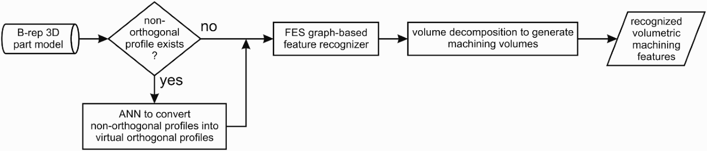
Fig. 10. The hybrid automatic feature recognition system approach (Wong & Lam, Reference Wong and Lam2000). 3-D, three-dimensional; FES, feature edge sequence; ANN, artificial neural network.
Li et al. (Reference Li, Ong and Nee2000) developed a system for automatic recognition of orthogonal interacting features based on a three-layer BP network, whose input was obtained by a combination of approaches based on graphs and hints. The training set consisted of 65 samples. The ANN had 20 neurons in the input layer, 11 neurons in the hidden one, and 6 in the output layer that were activated any time one of the following six features was recognized: cylindrical intrusions (the system did not separate blind and through holes), pockets, rectangular openings, slots, steps, or corner steps, which can be isolated or part of a complex feature.
Jun et al. (Reference Jun, Raja and Park2001) designed a system for reverse engineering with feature recognition based on a three-layer BP network. Three groups of parameters that have been formed semiautomatically based on 3-D scanned parts arrive on the input network layer of 9 neurons. Elements of a seven-dimension vector (seven digit code) arrive on neurons 1 to 7 indicating which edges are linked (forming contours). The convexity/concavity parameter arrives on input neuron 8, whereas the parameter of circularity/linearity arrives on neuron 9. The hidden layer consisted of 15 neurons, whereas the output one consisted of 6 that corresponded to recognitions of pockets, steps, protrusions, slots, holes, and blocks. The network was trained with the following parameters: η = 0.9, α = 0.5, and permitted error 10−4. The error value obtained fell below the permitted one after 70,000 input samples that completed the network training.
Ding and Yue (Reference Ding and Yue2004) developed a system of three-layer BP networks with three recognition levels. It is used only for new classes of interacting features. The network input is a FAM or a vertex adjacency matrix. Different input forms are treated with networks with different characteristics connected with the number of neurons in individual layers. Data exchange and classification principles were taken from the application protocol of the ISO 10303-224 STEP standard (ISO, 2001).
The final example of BP networks for AFR is related to the work of Öztürk and Öztürk (Reference Öztürk and Öztürk2001). In the early stages of the development of their system for AFR they used improved FSV as input into a four-layer BP network (Öztürk & Öztürk, Reference Öztürk and Öztürk2001). After a series of experiments with different topologies and parameters they obtained good results for simple and some more complex manufacturing features. However, the robust ANN structure required quite a lengthy and unstable network training process for new feature classes. In more recent work, Öztürk and Öztürk (Reference Öztürk and Öztürk2004) used the hybrid approach, which combined application of genetic algorithms for optimization of the input vector enabling a simpler architecture of the applied ANN for AFR: a three-layer BP network with seven neurons in the input and hidden layer and eight neurons in the output layer, whereas the training process is shorter and more stable.
The ANN-based feature recognition discussed in the literature review (Sunil & Pande, Reference Sunil and Pande2009) have various limitations. Most of the systems target a limited set of simple features such as rectangular pocket, blind/through step, and blind/through slot, which can be defined by four rectangular vertices or features with a fixed number of faces and so forth, and do not consider feature topology and geometry variations. Other systems use feature-specific representation schemes that have limitations such as ambiguity, nonuniqueness, and the need to have more networks for recognition, thus increasing the time and effort in training and testing the networks. Possible solution is related to the work of Sunil and Pande (Reference Sunil and Pande2009) based on an intelligent system for recognizing prismatic part machining features from B-rep CAD models using a BP neural network.
6.3. Hopfield's ANNs
Associative memory is a system enabling translation from the input space into the output space in a way that would tolerate errors, both in the degree of completeness and in acceptable noise levels in any possible input set form (Bose & Liang, Reference Bose and Liang1996). One of the main components of an intelligent system is the possibility of association of new forms of input data to those in the knowledge base and such memories are called autoassociative. One ANN that has such a property is Hopfield's.
A Hopfield network is a completely connected recurrent ANN whose topology is based on the following rule: output signals from all process elements act as input to one neuron, that means that there are no layers. They can be discrete and continual. Discrete use neurons with a linear input interaction function (the same applies to continual) and an impulse activation function (for discrete it is sigmoid). A discrete Hopfield network functions in the following way: in discrete time intervals t = 1, 2, … , one neuron is selected heuristically and its new output state is calculated.
The large number of reverse links opens the questions of stability conditions of these networks, that is, determining points in the state space to which trajectories vj(t) aim for (equilibrium points). Determination of connection weights can be performed by learning using Hebb's rules; but mathematical optimization is applied much more often, where the function of getting the system into equilibrium is set.
The time needed to get the system into a stable state is significant for practical implementation of these networks. Fu and Yan (Reference Fu and Yan1997) showed that the so-called Hopfield–Amari network reaches a stable state through maximally 40 iterations. It is an ANN with synchronous changes of state. The network input is defined with the contour bending function. Based on the value of this function by optimization the similarity coefficient 0 ≤ R ≤ 1 is determined for a model contour from the database and the investigated contour. Its values indicate whether the investigated contour and the model belong to the same class of contours. The system can recognize a great number of plane figures.
6.4. Kohonen's self-organizing maps (KSOMs)
Kohonen's ANNs use unsupervised learning. This type of learning is applied when input data is grouped into subgroups (clusters) according to an unknown criterion, so the error function cannot be formed. Thus, training cannot be supervised.
Kohonen's neural network together with the weight modification function makes a so-called KSOM shown in Figure 11.

Fig. 11. The Kohonen artificial neural network architecture. WTA, winner takes all.
The input layer of this network consists of n neurons v i(0) with a linear activation function. Outputs from this layer are taken to the input of a competing layer consisting of m neurons also with a linear activation function. Depending on the problem modeled by the network they are organized into 1-D, 2-D, or multidimensional fields. Response of the competing layer further acts as input to the so-called winner takes all network (Bose & Liang, Reference Bose and Liang1996) that has the same number of inputs and outputs as Kohonen's network. When in a trained KSOM the competing layer is excited, one neuron, a representative of the cluster the impulse belongs to, reacts the best (has the highest output signal). In the process of Kohonen's unsupervised learning the network is successively presented with training samples. Based on the index of the winning neuron, connection weights are modified.
Introduction of certain modifications into this procedure related to removing the need for normalization of the weight and excite vectors, method of selection of the winning neuron, and changing weights of all neurons spatially close to the winner, practical applicability of this network is attained and the training time is significantly reduced.
In Meeran and Zulkifli's (2002) system, a KSOM was applied for recognition of interacting nonorthogonal features. An xy graph in the form of a set of points, representing the resulting face obtained using the cross-sectional layer method is the ANN input. The recognition procedure is applied iteratively and each iteration assumes the following steps: (a) generation of maximal convex regions, (b) decomposition of the resulting surface into nonorthogonal regions (primitives), and (c) determining the remaining region. The resulting surfaces (resulting area) can be isolated primitives that do not need to be further decomposed, and graphs representing them are input into a three-layer BP network (Zulkifli & Meeran, Reference Zulkifli and Meeran1999a). In the case of the occurrence of interacting features the graph is input to the KSOM that has eight competing layers with two neurons. The number of iterations using KSOM depends on the feature complexity. Figure 12 illustrates recognition of a simple interacting feature, for which only one iteration was needed.

Fig. 12. An example of Kohonen self-organizing map (SOM) application for automatic feature recognition (Meeran & Zulkifli, Reference Meeran and Zulkifli2002).
6.5. ART neural networks
In networks with supervised learning, such as nonrecurrent, network retraining must be performed for every new input form that reduces their efficiency. ART ANNs, whose development started practically three decades ago, can store old inputs (sample forms) when learning new ones. Two types of these ANNs have been practically applied: ART-1 using the binary vector input form and ART-2 that processes analogous input forms.
The capability of input classification into different categories is built into the ART-1 network. The shortcoming of these networks is possible classification process instability if the input vector is not selected well enough that is reduced by selection of an appropriate learning algorithm. ART-1 networks, like Kohonen's are trained by unsupervised (competitive) learning, so the mechanism with the return links between the competitive and input layer is used for storing old, when new information is learned. Information between the input and competitive layer is sent forward or back until the network reaches a resonance state without which the learning process is not finished. The resonance state is realized very fast for previously learned input forms, and the memorized form is successfully updated. If the input form is not recognized at once the remaining memorized forms are searched fast and compared with it, so if it is not recognized the network goes into a resonance state in order to memorize that form as a new sample. The time relapsed until the resonance state is reached is much lower than the time needed to update connection weights between neurons of the input and competitive layer.
ART-1 has a two-layer structure (F1 and F2) and its neurons are interconnected via weight functions from bottom to top and top to bottom, as shown in Figure 13. In the competitive layer (layer F2) neurons compete for the chance to respond to the input form and the winning neuron represents a classification category of the input form. Competition takes place according to an algorithm that selects the winner, taking into account certain criterion or via prevention: inhibition of neurons of the competitive layer when the competitive layer is brought to a state where only the winning neuron is active. ART-1 has two subsystems: a learning subsystem and a subsystem for determining similarities. The learning subsystem contains an input and competitive neuron layer making up layers F1 and F2. Neurons in both layers are completely connected with neurons of the second level, and the learning subsystem establishes whether the input vector form is in association with the previously memorized forms.

Fig. 13. The structure of the adaptive resonance theory using the binary vector input form (ART-1) artificial neural network. LTM, long-term memory.
The subsystem for determining similarities is needed by the ART-1 network in order to determine the similarity of the input vector with the one that is known and successfully presented as part of the long-term memory or to form a new class of samples. The criterion for determining the similarity degree is represented with the so-called similarity parameter ρ, for which ρ ≤ 1. Selection of the value of this parameter is very important as it determined the “porosity” for classification of input vectors in the ART-1 neural network. This, for the given samples that need to be classified higher values of parameter ρ result in a finer discrimination between classes in relation to lower values of parameter ρ.
Differences between ART-2 and ART-1 reflect the changes necessary to adjust the network to continual input vectors. Level F1 of the ART-2 network is more complex as it includes normalization of the input vector and noise reduction. The system given in (Lankalapalli e al., 1997) is an example of the application of the ART-2 network for recognizing manufacturing features. Based on B-rep CAD models an FSV is formed. During training the similarity parameter value was between 0.9 and 0.99999 and complete separation of nine manufacturing features (tab, slot, rectangular protrusion, pocket, through hole, blind hole, cylindrical protrusion, cross-slot, step) was obtained for different levels of noise reduction and several combinations of these parameters.
7. CHARACTERISTICS OF OUTPUT DATA FROM ANNs IN SYSTEMS FOR AFR
The ANN output is the result of many operations performed over input data and weights and is a vector variable. Depending on the structure of the information carried by the output vector, three basic ANN output variants exist:
1. each neuron corresponds to one class of manufacturing features,
2. neurons carry more detailed information on the recognized form, and
3. matrix containing the code of the recognized manufacturing feature and machining direction.
An example of an output vector for which each neuron corresponds to one class of manufacturing features is found in the previously mentioned systems of Nezis and Vozniakos (1997; eight feature types, eight neurons in the output layer) and Chen and Lee (Reference Chen and Lee1998; six feature types, six neurons in the output layer).
The second variant of output data where the neuron carries detailed information on the recognized feature is found in the system of Hwang and Henderson (Reference Hwang and Henderson1992). They used six neurons as output and these neurons represent the class, name, reliability factor, name of the primary page, list of adjacent faces of the recognized feature, and total searching time.
An example for the last variant where the output vector is formed as a matrix containing the code of the recognized manufacturing feature and machining direction is found in the system of Zulkifli and Meeran (2002). The matrix is binary, with 2 × 5 dimensions. The first row in this matrix is kept for the code of the manufacturing feature in the shape of a five-digit binary number that enables in total 31 class of manufacturing features (11111(2) = 31(10)). The second row in the matrix is intended for the code for the tool approach direction during feature machining (+x, −x, +y, −y, −z). The digit “1” will appear on places corresponding to the approach direction, and the other places will be filled with “0.”
8. ADVANTAGES OF THE APPLICATION OF ANNs IN SYSTEMS FOR AFR
Compared to methods based on logic rules, application of ANNs in systems for automatic recognition of manufacturing features brings many advantages of which the following are the most important (Yue et al., Reference Yue, Ding, Ahmet, Painter and Walters2002; Ding & Mattews, 2009):
• ANNs tolerate slight errors in input data during the processes of problem training and solution.
• The recognition process is faster because it does not request long-term searching of the part representation structure or complex logical operations for obtaining necessary information, but instead requests simple mathematic calculations.
• They are capable of knowledge acquisition through the process of learning via examples that enable treatment of identified features for which there are no previously defined patterns in the knowledge base.
ANN techniques can eliminate a few drawbacks of conventional feature recognition methods (Yue et al., Reference Yue, Ding, Ahmet, Painter and Walters2002): the inability to recognize inexact or incomplete features, slow execution speed, and the inability to learn.
9. CONCLUSION
AFR is the first and most important step in translation of information defined by the CAD model into technologically applicable instructions. Elimination of the need for a manufacturing engineer for this task is essential for the development of a completely automatic CAPP system. Advantages of automatic recognition of manufacturing features in relation to DBFs are a significant saving of time and human resources by exchanging the human expert with a computer, and provision of the desired functionality of the designed part without limiting the creativity of design process with library availability of predefined manufacturing features. However, regardless of great scientific efforts this approach still suffers from numerous shortcomings (Lam & Wong, Reference Lam and Wong1999):
1. The complexity of recognition algorithms, especially in the case of interacting features: It is a huge problem to determine which features will be explicitly made and for which process plans are to be formed and which features will be implicitly made while machining some others.
2. The number of manufacturing feature types that can be efficiently recognized: A very small amount of research has been performed in the domain of nonorthogonal and arbitrary features.
3. Technological information carried by the recognized feature: This information is not enough for singular determination of the treatment type for its machining.
4. An all-inclusive algorithm: This type of algorithm that would provide complete automation of the process of manufacturing feature recognition does not exist.
This paper provided an extensive analysis of ANN-based feature recognition systems. The results are summarized in Table 2. ANN techniques have certain advantages over rule-based feature recognition methods:
1. ANN systems have the ability to learn and dynamically improve their performance.
2. A system with a trained network has significantly faster execution speed than a rule-based system that performs exhaustive searching for matching patterns each time.
3. An ANN-based feature recognition system has the ability to recognize and classify similar features, and there is no need to predefine all possible instances of features as in most rule-based systems.
Table 2. Overview of ANN-based AFR systems
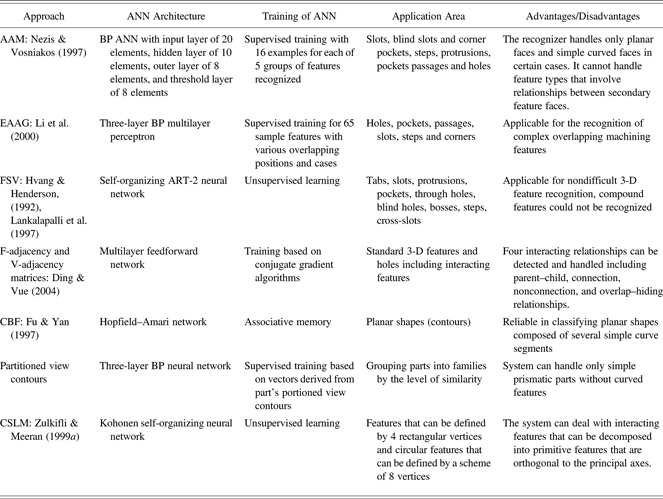
Note: ANN, artificial neural networks; AAM, attributed adjacency matrix; BP, backpropagation; EAAG, enhanced attributed adjacency graph; FSV, face score vector; ART-2, type of adaptive resonance theory that processes analogous input form; 3-D, three-dimensional; CBF, curve bend function; CSLM, cross-sectional layer method.
However, there are certain limitations:
1. Systems developed up till now are suitable for different individual applications, and they are far from a general AFR algorithm. Therefore, a limited range of features and feature intersections can be recognized.
2. Most ANN-based AFR systems employ supervised training. The weakness of such systems is, when an additional feature is presented to the network, the network has to be completely retrained with all training features.
3. Networks that have unsupervised training have plasticity (ability to learn new feature) and stability (ability for new learning not to be affected by previous learning; Lankalapalli et al., Reference Lankalapalli, Chatterjee and Chang1997). In contrast, AFR systems based on self-organizing ANNs have more limited applications than systems that use supervised training.
4. The knowledge base created by an ANN is not directly observable, so the basis for the output in response to any given input cannot be verified or examined directly.
Nevertheless, there are many advanced approaches, for example, Nezis and Vosniakos (Reference Nezis and Vosniakos1997), Jun et al. (Reference Jun, Raja and Park2001), and Ding and Yue (Reference Ding and Yue2004) using the STEP AP224 standard for data exchange and feature definition (ISO 10303-224; ISO, 2001). Encouraging results dealing with input representation and handling feature interactions can be found in Ding and Yue (Reference Ding and Yue2004) and Sunil and Pande (Reference Sunil and Pande2009). The potential of ANN techniques for feature recognition is clear. However, there is a need for further work. Newer research in the AFR field is thus directed toward the following:
• determination of more efficient algorithms for separation of necessary geometric information from CAD models and, of more significance, knowledge acquisition in the feature pattern library by applying ANNs and other advanced artificial intelligence techniques;
• incorporating new training methods;
• extending the range of the sectional geometry of features from rectangles and circles to more general shapes; and
• extending feature recognition abilities on lightweight representations (Ding & Matthews, Reference Ding and Matthews2009).
Bojan R. Babić is a Professor in the Production Engineering Department at the University of Belgrade and is Vice Dean of the Faculty of Mechanical Engineering. He lectures at all study levels and is the supervisor for a number of MS and PhD theses. He is experienced in project management and realization in the domain of technological development and for business enterprises at the national and international level. Dr. Babić has authored more than 80 papers in international journals and conference proceedings. His research interests include discrete event simulation, CAPP and computer-aided manufacturing, and intelligent manufacturing systems.
Nenad Nešić is a Teaching and Research Assistant in the Production Engineering Department at the University of Belgrade. He received his Dipl-Ing degree in mechanical engineering from the University of Belgrade in 1999. He has worked in the field of intelligent metrology and total quality management. His current areas of research interest include intelligent manufacturing systems and CAD, CAPP, and computer-aided manufacturing systems.
Zoran Miljković is a Professor in the Production Engineering Department at the University of Belgrade. He received MS and PhD degrees in mechanical engineering from the University of Belgrade, both in robotics and artificial neural networks. Dr. Miljković has authored more than 80 journal and conference papers and has published three books as well as several chapters in scientific monographs in manufacturing processes, mobile robotics, and artificial intelligence. His research interests include intelligent manufacturing systems and processes, robotics, machine learning, and ANNs.


