


1 Introduction
Near-wall turbulence is responsible for significant drag penalties in many flows of engineering relevance, and because of this, many researchers are studying various ways to be able to properly control the flow (Choi, Moin & Kim Reference Choi, Moin and Kim1993; Dubief et al. Reference Dubief, White, Terrapon, Shaqfeh, Moin and Lele2004; Orlandi & Leonardi Reference Orlandi and Leonardi2008; Rosti & Brandt Reference Rosti and Brandt2017; Rosti, Brandt & Pinelli Reference Rosti, Brandt and Pinelli2018b; Shahmardi et al. Reference Shahmardi, Zade, Ardekani, Poole, Lundell, Rosti and Brandt2019). Among the many control strategies, the use of polymers has been demonstrated to be very efficient to reduce drag in pipelines (Virk Reference Virk1971). Less attention has been given to more complex non-Newtonian fluids which can be found in a wide range of applications, including biological fluids and various industrial processes. One of the main features of these types of flows is the nonlinear relation between the shear stress and the shear rate. Here, we focus on fluids that can exhibit simultaneously elastic, viscous and plastic properties, usually called elastoviscoplastic (EVP) fluids (Balmforth, Frigaard & Ovarlez Reference Balmforth, Frigaard and Ovarlez2014). In particular, they behave as solids when the applied stress is below a certain threshold, the yield stress, while for stresses above it, they start to flow as liquids. The objective of this study is to apply recently developed tools from system dynamics, in particular higher order dynamic mode decomposition (HODMD), to turbulent channel flows to understand how the underlying turbulence dynamics is modified by plastic and elastic effects in the flow. By doing this, we will also show that HODMD is able to extract the relevant dynamics in Newtonian wall-bounded turbulence, a configuration so far quite elusive to this type of analysis owing to the complex interplay between the different temporal and spatial scales of the problem. Indeed, unlike homogeneous turbulence and free shear flows, production and dissipation of energy are associated with similar scales in wall-bounded flows (Cimarelli, De Angelis & Casciola Reference Cimarelli, De Angelis and Casciola2013; Cimarelli et al. Reference Cimarelli, De Angelis, Jimenez and Casciola2016).
In classical Newtonian flows, a regeneration cycle based on the growth and breakdown of streamwise elongated structures is known to sustain wall-bounded turbulence. This consists of the continuous extraction and momentum transfer from the outer region (high-velocity core) to the inner region (near wall, low velocity) and final dissipation into internal energy as an effect of the viscous forces. In particular, streamwise velocity streaks, which are elongated and narrow regions of excess or defect streamwise velocity, are generated by streamwise vortices via the lift-up effect (Moffatt Reference Moffatt, Yaglom and Tatarsky1967; Landahl Reference Landahl1980; Brandt Reference Brandt2014). These streaks break down and generate streamwise vorticity, completing the regeneration cycle which enables a turbulent flow to be sustained (Hamilton, Kim & Waleffe Reference Hamilton, Kim and Waleffe1995; Jiménez & Pineli Reference Jiménez and Pineli1999). The self-sustained mechanism is quantified statistically with the turbulent fluctuations and the Reynolds shear stress. Nevertheless, understanding the origin and stability of these coherent structures becomes important also to model and manipulate turbulence. Two key ingredients of this self-sustaining cycle are the lift-up mechanism and the streak breakdown. The lift-up mechanism has been found to be robust and ubiquitous in wall-bounded flows and it is associated with the generation of large energetic near-wall structures. The streaks, on the other hand, become unstable and break down via a rapid inviscid inflectional mechanism (Waleffe Reference Waleffe1995; Kawahara et al. Reference Kawahara, Jiménez, Uhlmann and Pinelli1998; Reddy et al. Reference Reddy, Schmid, Baggett and Henningson1998; Andersson et al. Reference Andersson, Brandt, Bottaro and Henningson2001). This instability has been initially treated as a modal secondary instability of long steady streaks, however, several authors proposed bypass mechanisms active also at lower streak amplitude, comparable to those found in turbulent flows. Schoppa & Hussain (Reference Schoppa and Hussain2002) suggested that the streak instability is indeed related to the transient growth of secondary perturbations, disrupting modally stable streaks (see also Höpffner, Brandt & Henningson (Reference Höpffner, Brandt and Henningson2005)); moreover, Brandt & de Lange (Reference Brandt and de Lange2008) show that, in a noisy environment, the interactions of finite length between streaks moving at different velocities is also able to initiate the streak breakdown, leading to vortical structures similar to those observed in simulations of turbulent channel flows. More recently, Cossu et al. (Reference Cossu, Brandt, Bagheri and Henningson2011) studied the nonlinear stability of laminar sinuously bent streaks in a plane Couette flow, showing that the transition to turbulence is induced by the initial transient amplification of streamwise vortices, forced by the decaying sinuous mode. This process is followed by a new growth of the streaks and their final breakdown. Here, we want to understand how the near-wall cycle is modified in an EVP fluid.
Significant attention has been given to viscoelastic flows to study turbulence modulation and near-wall structures in drag-reducing polymeric fluids. It has been shown that polymers can alter flow instabilities and transition to turbulence. Regarding stability, Biancofiore, Brandt & Zaki (Reference Biancofiore, Brandt and Zaki2017) examined the secondary instability of streaks in viscoelastic flows, showing that the streaks reach a lower average energy with increasing elasticity due to a resistive polymer torque that opposes the streamwise vorticity and, as a result, opposes the lift-up mechanism. Dubief et al. (Reference Dubief, Terrapon, White, Shaqfeh, Moin and Lele2005) studied the intermittency in turbulent viscoelastic flows, showing that the drag-reducing property of polymers is closely related to coherent turbulent structures. Polymers dampen near-wall vortices but also enhance streamwise kinetic energy in near-wall streaks. The net balance of these two opposite actions leads to a self-sustained drag-reduced turbulent flow. Recently, Xi & Graham (Reference Xi and Graham2010, Reference Xi and Graham2012a,Reference Xi and Grahamb) provided new insight into the mechanism by which polymer additives reduce the drag: they proposed that a turbulent flow is characterised by an alternate succession of strong and weak turbulence phases, the first characterised by flow structures showing strong vortices and wavy streaks, the latter weak streamwise vortices and almost streamwise-invariant streaks. In the Newtonian flow, the so-called active turbulence dominates, while active intervals becomes shorter while the so-called hibernating intervals are unaffected and become relatively more important with increasing viscoelasticity.
The stability of yield stress fluids has received increased attention during the last two decades (Nouar & Frigaard Reference Nouar and Frigaard2001; Metivier, Nouar & Brancher Reference Metivier, Nouar and Brancher2005; Nouar et al. Reference Nouar, Kabouya, Dusek and Mamou2007; Nouar & Bottaro Reference Nouar and Bottaro2010; Bentrad et al. Reference Bentrad, Esmael, Nouar, Lefevre and Ait-Messaoudene2017). Among these authors, Nouar et al. (Reference Nouar, Kabouya, Dusek and Mamou2007) found that, in a plane channel, the flow of an EVP fluid is always linearly stable. They showed that the unyielded regions (stress below the yield stress) always remain unyielded in a linear stability analysis, while the optimal disturbance for moderate or high Bingham number consists of an oblique wave, which is associated with the lift-up effect (Schmid Reference Schmid2007). Nouar & Frigaard (Reference Nouar and Frigaard2001) carried out a nonlinear stability analysis, showing that the critical Reynolds number for the transition from a laminar to turbulent flow increases with the Bingham number (the ratio between the yield and viscous stresses) and the nonlinear energy stability analysis has been recently extended to multi-layer flows of yield stress and viscoelastic fluids (Moyers-Gonzalez, Frigaard & Nouar Reference Moyers-Gonzalez, Frigaard and Nouar2004; Hormozi & Frigaard Reference Hormozi and Frigaard2012).
Efficient mixing of yield stress fluids is a difficult fundamental problem, because the solid regions are often merely convected by the surrounding fluid as rigid or elastic plugs. Previous studies of yield stress fluids have focused on the steady state at a low Reynolds number. However, despite that the actual flow in industrial applications and natural phenomena is often inertial and unsteady, numerical studies of turbulent yield stress fluids have appeared only recently (Rosti et al. Reference Rosti, Izbassarov, Tammisola, Hormozi and Brandt2018a). These authors studied the pressure drop and statistics of the turbulent channel flow for increasing values of the Bingham number and weak elasticity, from essentially Newtonian turbulence ( $Bi=0$) to relaminarisation. Velocity correlations show that the size of the near-wall streaks increases with the Bingham number, while it was suggested that the streaks are responsible for the interaction between the yielded and unyielded regions in the EVP flow.
Here, we will employ the results by Rosti et al. (Reference Rosti, Izbassarov, Tammisola, Hormozi and Brandt2018a) together with additional direct numerical simulations to disentangle the near-wall dynamics in turbulent elastoviscoplastic and viscoelastic fluid flows. To do so, we use the model proposed by Saramito (Reference Saramito2007) to simulate the elastoviscoplastic fluid and the widely used FENE-P model (Peterlin Reference Peterlin1966) for the viscoelastic fluid. While the latter is the most common choice for turbulent flows with polymers (Shahmardi et al. Reference Shahmardi, Zade, Ardekani, Poole, Lundell, Rosti and Brandt2019), the former was chosen to allow for the efficient three-dimensional and time evolving computations needed in a turbulent flow, which are currently not feasible with the pure Bingham model. Furthermore, the model proposed by Saramito (Reference Saramito2007) revealed the ability to capture additional relevant physics (Cheddadi et al. Reference Cheddadi, Saramito, Dollet, Raufaste and Graner2011; Fraggedakis, Dimakopoulos & Tsamopoulos Reference Fraggedakis, Dimakopoulos and Tsamopoulos2016) and to properly match experimental results and observations (Holenberg et al. Reference Holenberg, Lavrenteva, Shavit and Nir2012) (common materials used to study this type of EVP fluid are Carbopol solutions and liquid foams (Firouznia et al. Reference Firouznia, Metzger, Ovarlez and Hormozi2018; Zade et al. Reference Zade, Shamu, Lundell and Brandt2019)).
Via a nonlinear dynamic mode decomposition approach, we first identify the structures associated with the streak regeneration cycle in Newtonian turbulence, this being the first analysis of this kind to the authors’ knowledge. These structures consist of a group of travelling waves located near the channel wall. We then investigate how the near-wall streaks and coherent structures evolve as a function of the Bingham number, and determine which structures are characteristic of the unyielded and yielded regions. In particular, we wish to understand the relation between the flow coherent structures of different scales, and the relaminarisation found at high Bingham numbers, also looking at drag reduction in purely elastic fluids.
The method used for the analysis presented here is based on a variant of the now well-known dynamic mode decomposition (DMD) (Schmid Reference Schmid2010), denoted as HODMD (Le Clainche & Vega Reference Le Clainche and Vega2017a). This technique allows us to identify the nonlinear temporal dynamics in a non-Newtonian fluid, analysing data which are non-equidistant in time; also, the main benefit of HODMD lies in its ability to clean noisy data or filter small-amplitude frequencies (Le Clainche, Vega & Soria Reference Le Clainche, Vega and Soria2017b; Le Clainche et al. Reference Le Clainche, Moreno-Ramos, Taylor and Vega2018b), which makes this method suitable for the analysis of transient (Le Clainche & Vega Reference Le Clainche and Vega2017b; Le Clainche, Pérez & Vega Reference Le Clainche, Pérez and Vega2018c) or highly complex nonlinear flows. Similarly to DMD, HODMD decomposes spatio-temporal data into a group of modes that oscillate either in time, space or in time and space representing the leading flow dynamics as groups of travelling waves.
The article is organised as follows. Section 2 presents the description of the flow under investigation and § 3 introduces the HODMD algorithm and the methodology used to carry out the spatio-temporal analysis to detect the flow patterns. Sections 4 and 5 present our main results, with a comparison to a purely viscoelastic flow in § 6. Finally, § 7 presents the main conclusions of the present work.
2 Numerical simulations and flow description
This article presents the analysis and studies the flow structures of data from a direct numerical simulation of a turbulent channel flow of an incompressible fluid. We investigate three types of fluid: a Newtonian fluid, an elastoviscoplastic fluid in the limit of small elasticity, as in Rosti et al. (Reference Rosti, Izbassarov, Tammisola, Hormozi and Brandt2018a), and a purely viscoelastic fluid. This allows us to separate the effects of plasticity and elasticity on the turbulent wall cycle.
We consider an incompressible fluid governed by the Navier–Stokes equations
 $$\begin{eqnarray}\displaystyle & \displaystyle \unicode[STIX]{x1D735}\boldsymbol{\cdot }\boldsymbol{v}=0, & \displaystyle\end{eqnarray}$$
 $$\begin{eqnarray}\displaystyle & \displaystyle \unicode[STIX]{x1D70C}\left(\frac{\unicode[STIX]{x2202}\boldsymbol{v}}{\unicode[STIX]{x2202}t}+\boldsymbol{v}\boldsymbol{\cdot }\unicode[STIX]{x1D735}\boldsymbol{v}\right)=-\unicode[STIX]{x1D735}p+\unicode[STIX]{x1D735}\boldsymbol{\cdot }\unicode[STIX]{x1D707}_{f}(\unicode[STIX]{x1D735}\boldsymbol{v}+\unicode[STIX]{x1D735}\boldsymbol{v}^{\text{T}})+\unicode[STIX]{x1D735}\boldsymbol{\cdot }\unicode[STIX]{x1D749}, & \displaystyle\end{eqnarray}$$
 where  $\boldsymbol{v}$ and
  $p$ are the velocity and pressure fields,
  $\unicode[STIX]{x1D70C}$ and
  $\unicode[STIX]{x1D707}_{s}$ are the density and the solvent viscosity of the fluid and
  $\unicode[STIX]{x1D749}$ is an extra stress tensor describing the non-Newtonian behaviour. In the present study, the viscoelastic and elastoviscoplastic effects in the flow are reproduced by the extra stress tensor
  $\unicode[STIX]{x1D749}$ described by the FENE-P (Peterlin Reference Peterlin1966) and Saramito models (Saramito Reference Saramito2007), respectively, with a generic transport equation as
 $$\begin{eqnarray}\left(\frac{\unicode[STIX]{x2202}\boldsymbol{B}}{\unicode[STIX]{x2202}t}+\boldsymbol{v}\boldsymbol{\cdot }\unicode[STIX]{x1D735}\boldsymbol{B}-\boldsymbol{B}\boldsymbol{\cdot }\unicode[STIX]{x1D735}\boldsymbol{v}-\unicode[STIX]{x1D735}\boldsymbol{v}^{\text{T}}\boldsymbol{\cdot }\boldsymbol{B}\right)=\frac{a}{\unicode[STIX]{x1D706}}\unicode[STIX]{x1D644}-\frac{{\mathcal{F}}}{\unicode[STIX]{x1D706}}\boldsymbol{B},\end{eqnarray}$$
 where  $\unicode[STIX]{x1D706}$ and
  $\unicode[STIX]{x1D707}_{p}$ are the relaxation time and polymeric viscosity, respectively. The left-hand side of the equation is the so-called upper convective derivative, while the right-hand side represents the stretching of the polymers and the yielding criterion. In particular,
  $\boldsymbol{B}$,
  ${\mathcal{F}}$ and
  $a$ are equal to
  $\unicode[STIX]{x1D749}\unicode[STIX]{x1D706}/\unicode[STIX]{x1D707}_{p}+\unicode[STIX]{x1D644}$,
  $\text{max}(0,1-\unicode[STIX]{x1D70F}_{0}/|\unicode[STIX]{x1D749}^{d}|)$ and
  ${\mathcal{F}}$ in the Saramito model,
  $\unicode[STIX]{x1D749}^{d}$ being the deviatoric stress tensor, while they equal
  $(\unicode[STIX]{x1D749}\unicode[STIX]{x1D706}/\unicode[STIX]{x1D707}_{p}+a\unicode[STIX]{x1D644})/{\mathcal{F}}$,
  $L^{2}/(L^{2}-\text{trace}(\boldsymbol{B}))$ and
  $L^{2}/(L^{2}-3)$ in the FENE-P model. A fluid described by the Saramito model is subject to recoverable Kelvin–Voigt viscoelastic deformations when the local stress is below the yield stress
  $\unicode[STIX]{x1D70F}_{0}$, while when the local stress exceeds the yield value the fluid behaves as an Oldroyd-B viscoelastic fluid (
 ${\mathcal{F}}=a=1$, i.e. the right-hand side of the previous equation is null). The FENE-P fluid on the other hand is the natural extension of the Oldroyd-B valid for a higher level of elasticity, with the introduction of the parameter
  $L$, which represents the maximum extensibility of the polymers and is defined as the ratio of the length of a fully extended polymer dumbbell to its equilibrium length.
The numerical implementation used for solving elastoviscoplastic flows is presented and validated in full in Izbassarov et al. (Reference Izbassarov, Rosti, Ardekani, Hormozi, Brandt and Tammisola2018). This problem is characterised by five non-dimensional numbers. To ensure a fully developed flow, the bulk Reynolds number is fixed to  $Re_{b}=Uh/\unicode[STIX]{x1D707}_{0}=2800$, which corresponds to
  $Re_{\unicode[STIX]{x1D70F}}=180$ in the Newtonian case. The Bingham number,
  $Bi=\unicode[STIX]{x1D70F}_{0}h/\unicode[STIX]{x1D707}_{0}U$, characterising the ratio between the yield stress and the viscous forces, is varied in the range from
  $Bi=0$ (Newtonian flow) to
  $Bi=2.1$, to study the effect of plasticity on the coherent structures in this turbulent flow. Here,
  $\unicode[STIX]{x1D70F}_{0}$ is the yield stress of the EVP fluid,
  $U$ is the mean velocity (averaged over time and the spatial domain),
  $h$ is the half-channel height and
  $\unicode[STIX]{x1D707}_{0}=\unicode[STIX]{x1D707}_{f}+\unicode[STIX]{x1D707}_{p}$ is the total kinematic viscosity, where
  $\unicode[STIX]{x1D707}_{f}$ is the fluid viscosity and
  $\unicode[STIX]{x1D707}_{p}$ the polymeric contribution to dissipation. In these simulations, elastic effects are intentionally kept small by fixing the remaining parameters close to their Newtonian values: the Weissenberg number
  $Wi=\unicode[STIX]{x1D706}U/h=0.01$, where
  $\unicode[STIX]{x1D706}$ is the polymer relaxation time, and the fluid to total viscosity ratio is large (
 $\unicode[STIX]{x1D6FC}=\unicode[STIX]{x1D707}_{f}/(\unicode[STIX]{x1D707}_{f}+\unicode[STIX]{x1D707}_{p})=0.95$). It is remarkable that on keeping the same
  $Bi$ (in bulk units) and increasing
  $Re$, eventually the Newtonian results should be recovered, since
  $Bi$ in plus units (see Rosti et al. Reference Rosti, Izbassarov, Tammisola, Hormozi and Brandt2018a) is decreasing with
  $Re$ and for a sufficiently small value, it should not affect the flow anymore. The computational domain has the size
  $6h\times 2h\times 3h$ in the streamwise, wall-normal and spanwise directions, respectively. Periodic boundary conditions are imposed in the wall-parallel planes and there is no slip at the walls. For a full description of the numerical simulation set-up and algorithms, please consult Rosti et al. (Reference Rosti, Izbassarov, Tammisola, Hormozi and Brandt2018a) and Izbassarov et al. (Reference Izbassarov, Rosti, Ardekani, Hormozi, Brandt and Tammisola2018). The viscoelastic flows are obtained using the same numerical set-up and numerical method, with the FENE-P viscoelastic model replacing the EVP model.
In the following, we describe the main features of the elastoviscoplastic turbulent channel flow; the purely viscoelastic counterpart is well known from previous works, and some of them are mentioned in § 1. To provide a sense of the flow under consideration, figure 1 shows the variations of the streamwise vorticity in a representative wall-normal plane for the three Bingham numbers under investigation. The black region represents the unyielded regions of the EVP fluid. As the Bingham number is increased from zero, the areas where the flow is not yielded (solid regions) increase. At the same time, the complexity of the flow decreases, up to  $Bi=2.8$, when the flow is fully laminar (see Rosti et al. (Reference Rosti, Izbassarov, Tammisola, Hormozi and Brandt2018a) for more details). Note that the yielded regions are composed by small-scale structures, which maintain the complexity of the flow also at higher values of
  $Bi$.
$Bi$.

Figure 1. Contours of the instantaneous spanwise vorticity in the  $XY$ plane (
 $X$ horizontal and
  $Y$ vertical axes). Dark colour represents the areas where the flow is not yielded. (a–c)
  $Bi=0$, 1.4 and 2.1. Colours scale from
  $-3U_{b}/h$ (blue) to
  $3U_{b}/h$ (red).
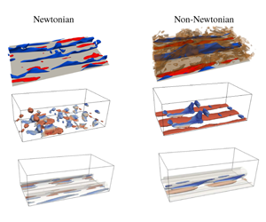
Figure 2(a–c) displays the iso-surfaces of the streamwise velocity fluctuations at the lower wall of the channel for the three Bingham numbers studied. At  $Bi=0$, it is possible to identify thin and elongated streaks, which are moving at either high or low speed (red and blue colour, respectively). When increasing the Bingham number, the number of high- and low-speed streaks decreases. The low-speed streaks seem to form a new single structure with a larger width, extending throughout the computational domain. The same type of structures are found close to the upper wall of the channel, as shown by the three cross-stream planes presented in figure 2(d–f). Rosti et al. (Reference Rosti, Izbassarov, Tammisola, Hormozi and Brandt2018a) found that these high-speed streaks penetrate to smaller wall-normal distances than their low-speed counterparts. The former are generally associated with wall-normal velocities towards the wall and with regions where the fluid is not yielded. In contrast, the fluid close to the low-speed streaks remains fully yielded. This description provides a general idea about the main flow structures present in the elastoviscoplastic flow, but it is necessary to carry out a more detailed analysis in order to deepen our understanding of the flow physics. In particular, we are interested in how and why the turbulent cycle is modified (and in some cases attenuated) in the non-Newtonian elastoviscoplastic and viscoelastic flows, compared to a Newtonian flow. This requires finding the interaction between the yielded and unyielded regions, the frequency of the flow leading modes, the phase velocity of structures travelling along the streamwise direction and the modification of the high- and low-speed streaks in these non-Newtonian flows.

Figure 2. Contours of the instantaneous streamwise velocity fluctuations (from the middle to the bottom part of the channel). The flow is from left to right. From left to right:  $Bi=0$, 1.4 and 2.1. (a–c) Streamwise velocity three-dimensional iso-surfaces in the lower channel wall. (d–f)
  $YZ$ plane (
 $Z$ horizontal and
  $Y$ vertical axes) extracted at
  $x=L_{x}/2$. Data normalised with their maximum value. Colour scales from
  $-0.6U_{b}$ to
  $0.6U_{b}$.
3 Methodology
3.1 HODMD
Higher order dynamic mode decomposition (Le Clainche & Vega Reference Le Clainche and Vega2017a) is an extension of DMD (Schmid Reference Schmid2010) that has been recently introduced for the analysis of complex flows, i.e. transition to turbulent flows in zero-net-mass-flux jets (Le Clainche et al. Reference Le Clainche, Vega and Soria2017b), identifications from noisy experimental data (Le Clainche et al. Reference Le Clainche, Sastre, Velazquez and Vega2017a,Reference Le Clainche, Vega and Soriab, Reference Le Clainche, Moreno-Ramos, Taylor and Vega2018b) or for the analysis of data acquired in a limited number of spatial locations (for example, field measurements, Le Clainche et al. (Reference Le Clainche, Moreno-Ramos, Taylor and Vega2018b), Le Clainche, Lorente & Vega (Reference Le Clainche, Lorente and Vega2018a)).
Similarly to DMD, this method decomposes spatio-temporal data  $\boldsymbol{v}(x,y,z,t_{k})$, collected at time instant
  $t_{k}$ (for convenience expressed as
  $\boldsymbol{v}_{k}$), as an expansion of
  $M$ modes
  $\boldsymbol{u}_{m}$, which are weighted by an amplitude
  $a_{m}$ as
 $$\begin{eqnarray}\boldsymbol{v}(x,y,z,t_{k})\simeq \mathop{\sum }_{m=1}^{M}a_{m}\boldsymbol{u}_{m}(x,y,z)\text{e}^{(\unicode[STIX]{x1D6FF}_{m}+\text{i}\unicode[STIX]{x1D714}_{m})t_{k}},\end{eqnarray}$$
 for  $k=1,\ldots ,K$. These modes oscillate in time with frequency
  $\unicode[STIX]{x1D714}_{m}$ and may grow, decay or remain neutral in time according to the growth rate
  $\unicode[STIX]{x1D6FF}_{m}$. To compute the HODMD algorithm, also called DMD-d, it is necessary firstly to collect and group together a set of
  $K$ time-equidistant snapshots
  $\boldsymbol{v}_{k}$ into a snapshot matrix of dimensions
  $J\times K$, where
  $J$ is the total number of grid points defining the spatial domain (in three-dimensional computational domains, assuming a uniform and structured mesh,
  $J=N_{x}\times N_{y}\times N_{z}$, where
  $N_{x}$,
  $N_{y}$ and
  $N_{z}$ are the number of points along the streamwise, normal and spanwise directions), in the following way:
 $$\begin{eqnarray}\unicode[STIX]{x1D651}_{1}^{K}=[\boldsymbol{v}_{1},\boldsymbol{v}_{2},\ldots ,\boldsymbol{v}_{k},\boldsymbol{v}_{k+1},\ldots ,\boldsymbol{v}_{K-1},\boldsymbol{v}_{K}].\end{eqnarray}$$
The HODMD algorithm can, for simplicity, be encompassed by two main steps, which will be reported briefly below. A more detailed description of the procedure can be found in Le Clainche & Vega (Reference Le Clainche and Vega2017a), Le Clainche et al. (Reference Le Clainche, Vega and Soria2017b).
3.1.1 Step 1: dimension reduction via singular value decomposition (SVD)
In order to remove spatial redundancies, filter out noise, etc., SVD is applied to the snapshot matrix (3.2). Based on a certain tolerance  $\unicode[STIX]{x1D700}_{1}$, the spatial dimension
  $J$ of the original snapshot data set is reduced to a set of linearly independent vectors of dimension
  $N$ (
$N$ ( $N<J$ is the spatial complexity) as
 $$\begin{eqnarray}\unicode[STIX]{x1D651}_{1}^{K}\simeq \unicode[STIX]{x1D652}\,\unicode[STIX]{x1D72E}\,\unicode[STIX]{x1D64F}^{\text{T}},\end{eqnarray}$$
 where the diagonal matrix  $\unicode[STIX]{x1D72E}$ contains the singular values
  $\unicode[STIX]{x1D70E}_{1},\ldots ,\unicode[STIX]{x1D70E}_{N}$ and
  $\unicode[STIX]{x1D652}^{\text{T}}\unicode[STIX]{x1D652}=\unicode[STIX]{x1D64F}^{\text{T}}\unicode[STIX]{x1D64F}$ are
  $N\times N$-unit matrices. The tolerance
  $\unicode[STIX]{x1D700}_{1}$ is a tuneable parameter set by the user, effectively determining the number
  $N$ of SVD modes retained as
 $$\begin{eqnarray}\unicode[STIX]{x1D70E}_{N+1}/\unicode[STIX]{x1D70E}_{1}\leqslant \unicode[STIX]{x1D700}_{1}.\end{eqnarray}$$
 The reduced snapshot matrix, of dimension  $N\times K$, is then defined from (3.3) as
 $$\begin{eqnarray}\widehat{\unicode[STIX]{x1D651}}_{1}^{K}=\unicode[STIX]{x1D72E}\,\unicode[STIX]{x1D64F}^{\text{T}},\end{eqnarray}$$
 with  $\unicode[STIX]{x1D651}_{1}^{K}=\unicode[STIX]{x1D652}\widehat{\unicode[STIX]{x1D651}}_{1}^{K}$.
3.1.2 Step 2: the DMD-d algorithm
The following high-order Koopman assumption is applied to the reduced snapshot matrix:
 $$\begin{eqnarray}\widehat{\unicode[STIX]{x1D651}}_{d+1}^{K}\simeq \widehat{\unicode[STIX]{x1D64D}}_{1}\widehat{\unicode[STIX]{x1D651}}_{1}^{K-d}+\widehat{\unicode[STIX]{x1D64D}}_{2}\widehat{\unicode[STIX]{x1D651}}_{2}^{K-d+1}+\cdots +\widehat{\unicode[STIX]{x1D64D}}_{d}\widehat{\unicode[STIX]{x1D651}}_{d}^{K-1},\end{eqnarray}$$
 where  $\widehat{\unicode[STIX]{x1D64D}}_{k}=\unicode[STIX]{x1D652}^{\text{T}}\unicode[STIX]{x1D64D}_{k}\unicode[STIX]{x1D652}$ for
  $k=1,\ldots ,d$. This equation divides the snapshot matrix into
  $d$ blocks. Each block contains
  $K-d$ snapshots, but time delayed. The previous equation is rewritten in terms of the modified snapshot matrix
  $\tilde{\unicode[STIX]{x1D651}_{1}}^{K-d+1}$ and the modified Koopman matrix
  $\tilde{\unicode[STIX]{x1D64D}}$ as
 $$\begin{eqnarray}\tilde{\unicode[STIX]{x1D651}}_{2}^{K-d+1}=\tilde{\unicode[STIX]{x1D64D}}\,\tilde{\unicode[STIX]{x1D651}}_{1}^{K-d},\end{eqnarray}$$
which can also be presented in the following way:
 $$\begin{eqnarray}\left[\begin{array}{@{}c@{}}\widehat{\unicode[STIX]{x1D651}}_{2}^{K-d+1}\\ \ldots \\ \widehat{\unicode[STIX]{x1D651}}_{d}^{K-1}\\[6.0pt] \widehat{\unicode[STIX]{x1D651}}_{d+1}^{K}\end{array}\right]=\left[\begin{array}{@{}cccccc@{}}\mathbf{0} & \unicode[STIX]{x1D644} & \mathbf{0} & \ldots & \mathbf{0} & \mathbf{0}\\ \boldsymbol{ 0} & \boldsymbol{ 0} & \unicode[STIX]{x1D644} & \ldots & \boldsymbol{ 0} & \boldsymbol{ 0}\\ \ldots & \ldots & \ldots & \ldots & \ldots & \ldots \\ \boldsymbol{ 0} & \boldsymbol{ 0} & \boldsymbol{ 0} & \ldots & \unicode[STIX]{x1D644} & \boldsymbol{ 0}\\ \widehat{\unicode[STIX]{x1D64D}}_{1} & \widehat{\unicode[STIX]{x1D64D}}_{2} & \widehat{\unicode[STIX]{x1D64D}}_{3} & \ldots & \widehat{\unicode[STIX]{x1D64D}}_{d-1} & \widehat{\unicode[STIX]{x1D64D}}_{d}\end{array}\right]\cdot \left[\begin{array}{@{}c@{}}\widehat{\unicode[STIX]{x1D651}}_{1}^{K-d}\\[6.0pt] \widehat{\unicode[STIX]{x1D651}}_{2}^{K-d+1}\\ \ldots \\ \widehat{\unicode[STIX]{x1D651}}_{d}^{K-1}\end{array}\right].\end{eqnarray}$$
 This matrix is expected to also exhibit redundancies that are eliminated by a new dimension reduction via truncated SVD using the tolerance  $\unicode[STIX]{x1D700}_{1}$ as
 $$\begin{eqnarray}\tilde{\unicode[STIX]{x1D70E}}_{N^{\prime }+1}/\tilde{\unicode[STIX]{x1D70E}}_{1}<\unicode[STIX]{x1D700}_{1},\end{eqnarray}$$
 where  $N^{\prime }>N$ is the number of retained SVD modes. In other words, the matrix organises the snapshot blocks identified in the high-order Koopman assumption in columns. In this way, it is possible to increase the spatial complexity of the data from
  $N$ to
  $N^{\prime }$, consequently extending the number of DMD modes calculated in the next step (defined as
  $M=\min (K,N^{\prime })$). For a sufficiently large number of snapshots
  $K$ (which is the common case), in cases in which the spatial complexity
  $N$ is smaller than the spectral complexity
  $M$ (for
  $K>N$), the high-order Koopman assumption completes the lack of spatial information (reduced to
  $N$) and ensures the good performance of the DMD method.
At this step, the modified snapshot matrix becomes
 $$\begin{eqnarray}\tilde{\unicode[STIX]{x1D651}}_{1}^{K-d+1}\simeq \tilde{\unicode[STIX]{x1D650}}\tilde{\unicode[STIX]{x1D72E}}\tilde{\unicode[STIX]{x1D64F}}^{\top }\simeq \tilde{\unicode[STIX]{x1D650}}\overline{\unicode[STIX]{x1D64F}}_{1}^{K-d+1},\end{eqnarray}$$
 with  $\overline{\unicode[STIX]{x1D64F}}_{1}^{K-d+1}=\tilde{\unicode[STIX]{x1D6F4}}\tilde{\unicode[STIX]{x1D64F}}^{\top }$, where
  $\tilde{\unicode[STIX]{x1D650}}^{\top }\tilde{\unicode[STIX]{x1D650}}=\tilde{\unicode[STIX]{x1D651}}^{\top }\tilde{\unicode[STIX]{x1D651}}$ are the
  $N^{\prime }\times N^{\prime }$-unit matrices, and the diagonal of matrix
  $\tilde{\unicode[STIX]{x1D72E}}$ contains the singular values
  $\tilde{\unicode[STIX]{x1D70E}}_{1},\ldots ,\tilde{\unicode[STIX]{x1D70E}}_{N^{\prime }}$. This step is completed via pre-multiplication of (3.7) by
  $\tilde{\unicode[STIX]{x1D650}}^{\top }$, which invoking (3.10) yields
 $$\begin{eqnarray}\overline{\unicode[STIX]{x1D64F}}_{2}^{K-d+1}=\overline{\unicode[STIX]{x1D64D}}\,\overline{\unicode[STIX]{x1D64F}}_{1}^{K-d}.\end{eqnarray}$$
 The new  $N^{\prime }\times N^{\prime }$-Koopman matrix is related to
  $\tilde{\unicode[STIX]{x1D64D}}$ by
  $\overline{\unicode[STIX]{x1D64D}}\simeq \tilde{\unicode[STIX]{x1D650}}^{\top }\tilde{\unicode[STIX]{x1D64D}}\tilde{\unicode[STIX]{x1D650}}$. Instead of computing this expression, we use the pseudoinverse in (3.11) by first applying SVD (no truncation) to the matrix
  $\overline{\unicode[STIX]{x1D64F}}_{1}^{K-d}$, as
 $$\begin{eqnarray}\overline{\unicode[STIX]{x1D64F}}_{1}^{K-d}=\unicode[STIX]{x1D650}\unicode[STIX]{x1D726}\unicode[STIX]{x1D651}^{\top },\end{eqnarray}$$
 where  $\unicode[STIX]{x1D650}\unicode[STIX]{x1D650}^{\top }=\unicode[STIX]{x1D650}^{\top }\unicode[STIX]{x1D650}=\unicode[STIX]{x1D651}^{\top }\unicode[STIX]{x1D651}$ are the
  $N^{\prime }\times N^{\prime }$-unit matrices and the diagonal of
  $\unicode[STIX]{x1D726}$ contains the
  $N^{\prime }$ singular values. The following equation
 $$\begin{eqnarray}\overline{\unicode[STIX]{x1D64D}}=\overline{\unicode[STIX]{x1D64F}}_{2}^{K-d+1}\unicode[STIX]{x1D651}\unicode[STIX]{x1D726}^{-1}\unicode[STIX]{x1D650}^{\top }\end{eqnarray}$$
 can be obtained substituting (3.12) into (3.11) and post-multiplying by  $\unicode[STIX]{x1D651}\unicode[STIX]{x1D726}^{-1}\unicode[STIX]{x1D650}^{\top }$. The
  $N^{\prime }$ eigenvalues
  $\unicode[STIX]{x1D707}_{m}$ and eigenvectors
  $\overline{\boldsymbol{q}}_{m}$ of
  $\overline{\unicode[STIX]{x1D64D}}$ permit computing of the reduced DMD expansion for the reduced snapshots (3.5) as follows:
 $$\begin{eqnarray}\widehat{\boldsymbol{v}}_{k}\simeq \mathop{\sum }_{m=1}^{M}\widehat{a}_{m}\widehat{\boldsymbol{u}}_{m}\text{e}^{(\unicode[STIX]{x1D6FF}_{m}+\text{i}\unicode[STIX]{x1D714}_{m})t_{k}},\end{eqnarray}$$
 for  $k=1,\ldots ,K$. We obtain the reduced DMD modes
  $\widehat{\boldsymbol{u}}_{m}$ (dimension
  $Nd$) by retaining only the first
  $N$ components of the vectors
  $\widehat{\boldsymbol{q}}_{m}=\tilde{\unicode[STIX]{x1D650}}\overline{\boldsymbol{q}}_{m}$. The frequencies
  $\unicode[STIX]{x1D714}_{m}$ and the damping rates
  $\unicode[STIX]{x1D6FF}_{m}$ are given by
 $$\begin{eqnarray}\unicode[STIX]{x1D6FF}_{m}+\text{i}\unicode[STIX]{x1D714}_{m}=\log (\unicode[STIX]{x1D707}_{m})/\unicode[STIX]{x0394}t.\end{eqnarray}$$
 Finally, the amplitudes  $\hat{a}_{m}$ are obtained via least squares fitting of (3.14), as in optimized DMD (Chen, Tu & Rowley Reference Chen, Tu and Rowley2012), which provides a suitable representation of the influence of each DMD mode on the general flow dynamics.
The original DMD expansion (3.1) is obtained, invoking (3.5), upon pre-multiplication of (3.14) by the matrix  $\unicode[STIX]{x1D652}$, and rescaling both the modes
  $\boldsymbol{u}_{m}$ and the amplitudes
  $a_{m}$ such that the modes exhibit unit norm.
Finally, the number of retained modes in the expansion (3.1),  $M$, which is the spectral complexity, is determined using a second tolerance
  $\unicode[STIX]{x1D700}_{2}$, also tuneable, as
 $$\begin{eqnarray}a_{M+1}/a_{1}\leqslant \unicode[STIX]{x1D700}_{2}.\end{eqnarray}$$
The error made in the calculations is measured by the root mean square (r.m.s.) error of the HODMD reconstruction (3.1), calculated as
 $$\begin{eqnarray}RMSE=\sqrt{\frac{\mathop{\sum }_{k=1}^{K}||\boldsymbol{v}_{k}-\boldsymbol{v}_{k}^{DMD}||^{2}}{\mathop{\sum }_{k=1}^{K}||\boldsymbol{v}_{k}||^{2}}},\end{eqnarray}$$
 where  $||\cdot ||$ is the usual Euclidean norm.
3.2 Some remarks on the HODMD algorithm
The algorithm previously presented is similar to standard DMD (Schmid Reference Schmid2010) when the parameter  $d=1$ in the high-order Koopman assumption (3.6). HODMD provides the same results as DMD in the analysis of periodic solutions, linear flows (Gómez et al. Reference Gómez, Clainche, Paredes, Hermanns and Theofilis2012) or experimental saturated flows (Schmid Reference Schmid2011). Thus the main goal of this high-order algorithm is to serve as an extension that should be used in cases in which standard DMD experiences some difficulties (i.e. noisy experimental data, see Le Clainche et al. Reference Le Clainche, Vega and Soria2017b), or even fails, in particular when the spectral complexity
  $M$ is larger than the spatial complexity
  $N$ (more details in Le Clainche & Vega Reference Le Clainche and Vega2017a).
The tolerance  $\unicode[STIX]{x1D700}_{1}$ determines the number
  $N$ of SVD modes retained in Step 1 of the algorithm. This tolerance varies with the type of analysis carried out. For example, in noisy data, this tolerance should be equivalent to the level of noise. In complex flows (i.e. transitory or turbulent) the level of tolerance filters out the small-amplitude modes. As will be detailed in § 4.1, it is necessary to calibrate the parameters (
 $\unicode[STIX]{x1D700}_{1}$,
  $\unicode[STIX]{x1D700}_{2}$,
  $d$) before applying the method. This step is crucial for obtaining robust and accurate results.
The proved high efficiency of HODMD is due to the sliding window process applied to the snapshot matrix (3.2) by the DMD-d algorithm, see equation (3.6) and the sketch in figure 3. This window shift can be related to the well-known technique of power spectral density (PSD), which divides the data into several small segments, also known as windows, to perform fast Fourier transform (FFT) locally in each one of the segments. Then, the group of frequencies calculated locally in each segment is promediated. The result is a single group of averaged frequencies, representing all the FFT analyses carried out in the several segments. These average values are representative of the complete data set (this result is comparable to the frequencies calculated applying FFT to the complete data set, but the average values calculated with the PSD algorithm provides smoother results). In HODMD,  $d$ represents the number of segments. Solving the eigenvalue problem of a matrix containing the
  $d$ Koopman operators, which connect the different groups of snapshots (3.8), supplies the modified Koopman matrix with some specific properties: (i) noise cleaning, (ii) higher accuracy calculations, (iii) the ability to approximate solutions when the data analysed are not equispaced in time. Similarly to PSD, the search for a single and common solution satisfying simultaneously all the snapshot groups allows for averaged values, which are robust and suitably describe the main flow dynamics.

Figure 3. Sketch representing the snapshot matrix and the DMD-d sliding window process defined in (3.6).
In order to clean the data analysed and obtain high accuracy solutions, the algorithm HODMD is applied iteratively. In other words, once the main DMD modes, frequencies, growth rates and amplitudes are calculated, the original data are reconstructed as in the expansion (3.1). Then, the method is applied again over this reconstruction, which in principle only contains the main (filtered) dynamics. The same process is repeated several times, until the number of modes retained in the expansion (3.1) is kept constant. For the data analysed in this article, this iterative process is combined with the multi-resolution DMD-d algorithm. This algorithm, described in Le Clainche et al. (Reference Le Clainche, Vega and Soria2017b), presents a more efficient version of HODMD, suitable for the analysis of multi-dimensional complex data. This multi-resolution DMD-d algorithm uses a high-order singular value decomposition (HOSVD) (Tucker Reference Tucker1966) instead of classic SVD in Step 1 of the method. In detail, instead of organising the data in the snapshot matrix (3.2), they are organised in tensor form  $\unicode[STIX]{x1D61D}(x_{i},y_{l},z_{r},t_{k})=\unicode[STIX]{x1D61D}_{ilrk}$ (for
  $i=1,I$;
  $l=1,L$;
  $r=1,R$;
  $k=1,K$ with
  $I$,
$I$,  $L$ and
  $R$ the number of grid points related to the spatial components
  $x$,
$x$,  $y$,
$y$,  $z$ and where
  $K$ is the snapshot number). By applying standard SVD to the four matrices whose columns are formed by each one of the 4 data variables (similar to the fibres of a tensor), this method provides the following decomposition
 $$\begin{eqnarray}\unicode[STIX]{x1D61D}_{ilrk}\simeq \mathop{\sum }_{p_{1}=1}^{P_{1}}\mathop{\sum }_{p_{2}=1}^{P_{2}}\mathop{\sum }_{p_{3}=1}^{P_{3}}\mathop{\sum }_{n=1}^{N}\unicode[STIX]{x1D61A}_{p_{1}p_{2}p_{3}n}\unicode[STIX]{x1D61E}_{ip_{1}}^{(x)}\unicode[STIX]{x1D61E}_{lp_{2}}^{(y)}\text{W}_{rp_{3}}^{(z)}\unicode[STIX]{x1D61B}_{kn},\end{eqnarray}$$
 where  $\unicode[STIX]{x1D61A}_{p_{1}p_{2}p_{3}n}$ is a fourth-order tensor (called the core tensor) and the columns of the matrices
  $\unicode[STIX]{x1D652}^{(x)}$,
  $\unicode[STIX]{x1D652}^{(y)}$,
  $\unicode[STIX]{x1D652}^{(z)}$ and
  $\unicode[STIX]{x1D64F}$ are known as the modes of the decomposition (three spatial modes and one temporal mode, respectively). The reduction in equation (3.4) is then applied to each one of these modes, allowing for a better cleaning in every spatial and temporal direction. Finally, Step 2 is applied over the temporal modes
  $\unicode[STIX]{x1D64F}$.
3.3 Spatio-temporal modal decomposition
The main goal of this DMD decomposition is to study the spatio-temporal structures in terms of travelling waves  $\widehat{\boldsymbol{u}}_{mn}$ with defined spatial wavenumbers
  $\unicode[STIX]{x1D6FC}_{mn}$ and
  $\unicode[STIX]{x1D708}_{mn}$, which oscillate and grow/decay in time,
 $$\begin{eqnarray}\boldsymbol{v}(x_{j},y,z,t_{k})\simeq \mathop{\sum }_{m,n=1}^{M,N}a_{mn}\widehat{\boldsymbol{u}}_{mn}(y,z)\text{e}^{(\unicode[STIX]{x1D6FF}_{m}+\text{i}\unicode[STIX]{x1D714}_{m})t_{k}+(\unicode[STIX]{x1D708}_{mn}+\text{i}\unicode[STIX]{x1D6FC}_{mn})x_{j}},\end{eqnarray}$$
 for  $k=1,\ldots ,K$ and
  $j=1,\ldots ,J$. This expansion can be easily obtained by simply applying HODMD to the DMD modes in (3.1), resulting in the following DMD expansion
 $$\begin{eqnarray}\boldsymbol{u}_{m}(x_{j},y,z)\simeq \mathop{\sum }_{n=1}^{N}a_{n}\widehat{\boldsymbol{u}}_{mn}(y,z)\text{e}^{(\unicode[STIX]{x1D708}_{mn}+\text{i}\unicode[STIX]{x1D6FC}_{mn})x_{j}},\end{eqnarray}$$
 for  $j=1,\ldots ,J$. Equation (3.19) is obtained by combining this solution with (3.1), where the spatio-temporal amplitudes are defined as
  $a_{mn}=a_{m}a_{n}$. In a similar way, it is possible to obtain spatio-temporal expansions along the remaining spatial directions. For example,
 $$\begin{eqnarray}\boldsymbol{v}(x,y,z_{r},t_{k})\simeq \mathop{\sum }_{m,n=1}^{M,N}a_{mn}\bar{\boldsymbol{u}}_{mn}(x,y)\text{e}^{(\unicode[STIX]{x1D6FF}_{m}+\text{i}\unicode[STIX]{x1D714}_{m})t_{k}+(\unicode[STIX]{x1D706}_{mn}+\text{i}\unicode[STIX]{x1D6FD}_{mn})z_{r}},\end{eqnarray}$$
 for  $k=1,\ldots ,K$ and
  $r=1,\ldots ,R$, where
  $\unicode[STIX]{x1D706}_{mn}$ and
  $\unicode[STIX]{x1D6FD}_{mn}$ are the growth rates and wavenumbers related to the spanwise direction. Using this expansion, it is also possible to describe the data analysed as a group of travelling waves whose phase velocity is defined as
  $c_{mn}=\unicode[STIX]{x1D714}_{m}/\unicode[STIX]{x1D6FD}_{mn}$. A more detailed description of the method can be found in Le Clainche et al. (Reference Le Clainche, Pérez and Vega2018c), Le Clainche & Vega (Reference Le Clainche and Vega2018).
3.4 Modified Koopman operator for the analysis of data non-equidistant in time
The properties of the modified Koopman matrix for the analysis of data non-equidistant in time is illustrated by the following toy model
 $$\begin{eqnarray}f(t)=\sqrt{\cos (\unicode[STIX]{x1D714}_{1}t)\sin (\unicode[STIX]{x1D714}_{2}t)+2},\end{eqnarray}$$
 where  $\unicode[STIX]{x1D714}_{1}=\sqrt{2}$ and
  $\unicode[STIX]{x1D714}_{2}=1$, which exhibit the incommensurable fundamental frequencies
  $\unicode[STIX]{x1D714}_{1}\pm \unicode[STIX]{x1D714}_{2}$ and their multiple harmonics. The spatial dimension and complexity of this toy model is
  $1$ (single point in space), while the spectral complexity (number of frequencies) is incommensurable, and it will be approximated by the
  $M$ terms retained in the DMD expansion (3.1).
Applying HODMD, using the tolerances  $\unicode[STIX]{x1D700}_{1}=\unicode[STIX]{x1D700}_{2}=3\times 10^{-3}$, to a set of data composed by
  $K=400$ snapshots (spectral dimension), equidistant in time
  $\unicode[STIX]{x0394}t=10^{-1}$, the method approximates the original solution with the r.m.s. error ∼4. 5 × 10⁻³ (order of the tolerances) retaining
  $M=9$ modes. These are the
  $4$ frequencies
  $\unicode[STIX]{x1D714}_{1}+\unicode[STIX]{x1D714}_{2}$,
  $\unicode[STIX]{x1D714}_{1}-\unicode[STIX]{x1D714}_{2}$,
  $2\unicode[STIX]{x1D714}_{1}$ and
  $2(\unicode[STIX]{x1D714}_{1}-\unicode[STIX]{x1D714}_{2})$, which are calculated exactly until the fifth decimal point (in good agreement with the values of
  $\unicode[STIX]{x1D700}_{1}$ and
  $\unicode[STIX]{x1D700}_{2}$), their conjugate complex and the mode with zero frequency,
  $\unicode[STIX]{x1D714}_{0}$. In these calculations
  $d=120$, although it is remarkable that similar results are obtained using values of
  $100\leqslant d\leqslant 290$. For values of
  $d\leqslant 10$ the method miscalculates the frequencies and may add spurious elements (i.e. using
  $d=10$ the reconstruction error is ∼10-1).

Figure 4. Variations of the time interval between snapshots in toy model (3.22).
Next, the method is applied to analyse the same amount of data ( $K=400$ snapshots), but not-equidistant in time. The time interval at which the data are collected varies randomly between each snapshot, from
  $\unicode[STIX]{x0394}t_{min}=5\times 10^{-3}$ to
  $\unicode[STIX]{x0394}t_{max}=1.97\times 10^{-1}$, as seen in figure 4. However, the HODMD algorithm considers a set of data equidistant in time. To satisfy this constraint, the approximated time interval is calculated as the average between the minimum and maximum values of the varying time interval,
  $\unicode[STIX]{x0394}t=(\unicode[STIX]{x0394}t_{max}+\unicode[STIX]{x0394}t_{min})/2\simeq 10^{-1}$. The temporal-disparity ratio, defined as
  $TDR=(\unicode[STIX]{x0394}t_{max}-\unicode[STIX]{x0394}t_{min})/\unicode[STIX]{x0394}t\simeq 1.9$, shows the diversity in the collection of the snapshots in time. The HODMD has been applied using the same tolerance as in the previous case for
  $d=100$,
  $d=200$ and
  $d=290$. In all these cases, the method is able to capture the dominant frequencies
  $\unicode[STIX]{x1D714}_{1}\pm \unicode[STIX]{x1D714}_{2}$, but it also calculates some spurious modes. These modes are easily distinguishable, since their values change with the value of
  $d$, as shown in figure 5(a) that compares the exact solution with the present results. The original function is reconstructed using only the 2 modes
  $\unicode[STIX]{x1D714}_{1}\pm \unicode[STIX]{x1D714}_{2}$ and the mode
  $\unicode[STIX]{x1D714}_{0}$ with an r.m.s. error of 1. 2 × 10⁻² for the three values of
  $d$ considered. Figure 5(b) compares the function with the aforementioned reconstructions and table 1 summarises the number of modes computed in each case and the relative error made in the frequency calculations, which is ∼10-2 in all cases.

Figure 5. Results of DMD-d applied to  $400$ snapshots with variable time interval for the toy model (3.22). Black, red, blue and pink colours correspond to the exact solution, and to the solution obtained using
  $d=100$, 200 and 290. (a) Frequency versus amplitude of the DMD modes. (b) Reconstruction of the toy model signal using the frequencies
  $\unicode[STIX]{x1D714}_{1}\pm \unicode[STIX]{x1D714}_{2}$ and
  $\unicode[STIX]{x1D714}_{0}$.
Table 1. Results of the DMD-d used to approximate the toy model in (3.22). The data consist of 400 snapshots with time interval varying as in figure 4. The table shows the number of modes retained in the calculations, the values of the fundamental frequencies and their relative errors compared with the exact solutions  $\unicode[STIX]{x1D714}_{1}-\unicode[STIX]{x1D714}_{2}\simeq 2.4142$ and
  $\unicode[STIX]{x1D714}_{1}+\unicode[STIX]{x1D714}_{2}\simeq 0.4142$.

It is also possible to note from figure 5(a) that the modes with frequencies  $2\unicode[STIX]{x1D714}_{1}$ and
  $2(\unicode[STIX]{x1D714}_{1}-\unicode[STIX]{x1D714}_{2})$ are approximated in the 3 analyses with a relative error smaller than ∼10-2. Although the error made in the calculations of the mode amplitudes is much larger than for the frequencies (∼3 × 10⁻¹), it should be considered that the order of magnitude of the amplitudes is ∼10-3, meaning that these differences are almost negligible when reconstructing the original solution, with the r.m.s. error being ∼10-2 in all cases. Table 2 summarises the frequency of the two smaller-amplitude modes for the three analyses carried out; in some cases the error made in the calculations is even smaller than ∼10-2.
Table 2. Same as table 1 for the two smaller amplitude modes with frequencies  $2\unicode[STIX]{x1D714}_{1}\simeq 2.8302$ and
  $2(\unicode[STIX]{x1D714}_{1}-\unicode[STIX]{x1D714}_{2})\simeq 1.9993$.

The previous analysis has been repeated adding 10 % of random noise to the toy model (3.22) to show how the analysis can capture the underlying signal. The distance between snapshots is maintained as shown in figure 4 and the parameters used are the same as before ( $\unicode[STIX]{x1D700}_{1}=\unicode[STIX]{x1D700}_{2}=3\times 10^{-3}$ and
  $d=100$, 200, 290). As in the previous case, the method retains a large number of spurious modes; nevertheless, it is possible to distinguish the two fundamental frequencies
  $\unicode[STIX]{x1D714}_{1}\pm \unicode[STIX]{x1D714}_{2}$ from the remaining modes, since they are the only consistent frequencies in all three analyses. However, due to the large level of noise, the method is not able to retain the two lower-amplitude modes. The signal is reconstructed using the modes
  $\unicode[STIX]{x1D714}_{1}\pm \unicode[STIX]{x1D714}_{2}$ and
  $\unicode[STIX]{x1D714}_{0}$, with a r.m.s. error of 1. 2 × 10⁻² for the three values of
  $d$, as shown in figure 6, which compares the clean and noisy signal with the DMD-d reconstruction. Table 3 summarises the total number of modes and the relative error made in the frequency calculations for the noisy signal, which is ∼10-2, despite the noise added.

Figure 6. DMD-d applied in the toy model (3.22) with variable time interval between snapshots and 10 % of additional random noise. (a) Black dashed line: original clean solution, red line: original signal with noise and blue line: reconstruction using  $\unicode[STIX]{x1D714}_{1}\pm \unicode[STIX]{x1D714}_{2}$ with
  $100\leqslant d\leqslant 300$. (b) Zoom of the left figure.
Table 3. Same as table 1 for the signal with random noise.

Note finally that more calculations have been carried out using different non-equidistant time intervals to construct the snapshot matrix of the toy model (3.22) and the results obtained for the clean and noisy signals are similar to the one presented here. In addition, the same test has been successfully performed for variations of the toy model (3.22), although not reported here for the sake of brevity. To summarise, the example presented in this section shows that HODMD is suitable to study data that are non-equidistant in time. HODMD is able to (i) calculate the leading modes with high accuracy and (ii) approximate the frequencies of the lower-amplitude modes.
4 Coherent structures in the Newtonian and elastoviscoplastic turbulent channel flows
4.1 Initial calibration and parameter selection
The large number of frequencies and spatio-temporal scales typical of turbulent flows complicate the detection of flow patterns. It is therefore important to assess the robustness of the results, as in the toy model above. Thanks to the favourable properties of the modified Koopman operator, which defines a solution that is satisfied in all the sub-groups of data (snapshots) analysed simultaneously, it is possible to identify the large-scale and large-amplitude modes from a number of fairly disparate frequencies found in the flow. To this end, DMD-d is applied with different tolerances and various values of the parameter  $d$. In the problem studied in this paper, two distinct regions exist, defined by yielded and unyielded flow, where the flow moves at different velocities and presents different properties. This distinction encourages us to normalise the DMD modes with two norms, related with the maximum and the average values of the velocity field: the infinity norm (
 $L_{\infty }$) and the
  $L_{2}$ norm. The modes related to large-scale structures describing the flow physics will therefore be sought using different tolerances, values of
  $d$ and different types of normalisation (see also Le Clainche et al. (Reference Le Clainche, Moreno-Ramos, Taylor and Vega2018b)).
Figure 7 shows the frequency versus the amplitude of the different modes obtained with DMD-d using several different parameters for the three Bingham numbers studied. Even though it is possible to obtain a large number of modes for each case, only a few are robust; in other words, only a few frequencies are found in all the calculations performed: these form clusters of modes, as highlighted in the figure. To identify these clusters it is necessary that, in at least 8 (75 %) of a total of 12 calculations performed using HODMD, the solution provides modes with a frequency value defined as  $|f_{mi}-f_{mj}|<\unicode[STIX]{x1D716}$, where
  $f_{mi}$ and
  $f_{mj}$ represent the frequencies obtained in two different test cases, and
  $\unicode[STIX]{x1D716}$ is a tolerance defined by the user. This tolerance is set to
  $\unicode[STIX]{x1D716}=10^{-3}$ (one order of magnitude larger than the largest
  $\unicode[STIX]{x1D700}_{1}$ set in HODMD) for the cases
  $Bi=0$ and 1.4 (for which we use 66 snapshots) and
  $\unicode[STIX]{x1D716}=2\times 10^{-3}$ for the case
  $Bi=2.1$ (for which we use 35 snapshots). The high complexity of the flow and the fact that the data are not equidistant in time complicates the calculation of these modes, which is reflected in small differences in the values of the amplitudes and frequencies computed. The relative error assumed in the calculations of these frequencies is ∼10-2 (relative to the mean frequency of each group of robust modes) for the cases at
  $Bi=0$ and
  $Bi=1.4$ and ∼3. 5 × 10⁻² for
  $Bi=2.5$. Variations in the amplitudes are larger, nevertheless, these do not affect the DMD modes (they present similar shape and small variations in the order of magnitude), but only their weight in the DMD expansion (3.1). Since the purpose of this article is to gain insight into the flow physics, rather than to build a reduced-order model based on (3.1) (see Le Clainche & Vega (Reference Le Clainche and Vega2017b) for more details), the error made in the amplitude calculations is not further considered. The amplitude associated with each mode is estimated as the mean value for each cluster of modes. Considering the small error made in the frequency calculations and the similarities in the shape and the order of magnitude of the DMD modes calculated for each case (variations ∼10-2), this average value is considered to be sufficiently good to represent the influence of each mode on the flow dynamics.

Figure 7. DMD-d calibration. Amplitude normalised with the maximum value ( $\hat{a}_{m}=a_{m}/a_{0}$) versus frequency (
 $f_{m}=\unicode[STIX]{x1D714}_{m}/(2\unicode[STIX]{x03C0})$) obtained with different tolerances and order
  $d$ for
  $Bi=0$ (a),
  $Bi=1.4$ (b) and
  $Bi=2.1$ (c). For all cases,
  $\unicode[STIX]{x1D700}_{2}=10^{-3}$. Squares and triangles correspond to
  $\unicode[STIX]{x1D700}_{1}=10^{-6}$, circles and crosses correspond to
  $\unicode[STIX]{x1D700}_{1}=10^{-4}$. Blue, black and red colours correspond to
  $d=15$, 20, 25 for
  $Bi=0$ and 1.4 (
 $K=66$ snapshots) and
  $d=8$, 10, 15 for
  $Bi=2.1$ (
 $K=35$ snapshots). Circles and squares denote modes normalised with the
  $L_{\infty }$ norm. Crosses and triangles: modes normalised with the
  $L_{2}$ norm.
It is noteworthy that increasing the Bingham number reduces the flow complexity, so that similar solutions are obtained using a smaller number of snapshots. Although the accuracy of the estimated frequency decreases and its value is more sensitive to the choice of  $d$, obtaining good results using a smaller number of snapshots (yet in a turbulent flow) enables us to obtain a good compromise between computational cost and accuracy. Four main points should be emphasised from the calibration: (i) the number of snapshots used in each one of these calculations is
  $K=66$ for the cases with
  $Bi=0$ and
  $Bi=1.4$, and
  $K=35$ for the case with
  $Bi=2.1$, (ii) the parameter
  $d$ is proportional to the number of snapshots used in the analyses (if the number of snapshots is reduced by half,
  $d$ should be reduced by half, see more details in Le Clainche & Vega Reference Le Clainche and Vega2017a), (iii) in all cases, the time interval between snapshots varies within
  $(\unicode[STIX]{x0394}t_{min},\unicode[STIX]{x0394}t_{max})\simeq (1.8\times 10^{-3}\unicode[STIX]{x0394}S,2.1\times 10^{-3}\unicode[STIX]{x0394}S)$, where
  $\unicode[STIX]{x0394}S=4000$ is the time step interval at which the snapshots are saved during the numerical simulations, and the temporal-disparity ratio is ∼0. 12 (much smaller than in the toy model example), (iv) the averaged time interval
  $\unicode[STIX]{x0394}t$ determines the frequencies calculated. The flexibility of this iterative multi-resolution HODMD algorithm, which is able to provide robust results using data that are non-equidistant in time, makes it possible to use results from simulations using variable time steps and the data saved at fixed time step intervals. The large computational cost of these simulations makes it expensive to repeat the calculations. Therefore, the ability to use existing data constitutes a clear advantage.

Figure 8. Frequency versus amplitude from the DMD-d analysis of EVP fluids at  $Bi=0$, 1.4 and 2.1; also displayed with
  $\ast$ is the result of the analysis carried out on the EVP function for
  $Bi=2.1$.
Table 4. Frequencies and amplitudes of the DMD modes presented in figure 8. The modes are organised from lower to higher frequency from top to bottom.

4.2 Global temporal modes
The spectrum of the temporal DMD modes identified in the calibration process presented in the previous section is shown in figure 8, which compares the frequencies and the amplitudes of the modes calculated for Newtonian flow ( $Bi=0$) and for two finite Bingham numbers.
From figure 8 it is possible to identify six groups of modes. Table 4 summarises the frequencies and amplitudes of the modes. For the Newtonian turbulent flow, we obtain three types of modes named  $F1$,
$F1$,  $F2$ and
  $F3$ (where
  $F$ stands for fluid), while at finite Bingham number we also find three new type of modes,
  $S1$,
$S1$,  $S2$ and
  $S3$ (where
  $S$ stands for solid);
  $S1$ is characterised by a lower frequency than
  $F1$, confirming that streaks are on average sustained longer. The amplitude of the
  $S$ modes increases with the Bingham number, meaning that their activity becomes stronger when the volume of the unyielded flow increases. In contrast, the amplitude of mode
  $F3$ slightly increases from
  $Bi=0$ to
  $Bi=1.4$, but strongly decreases at
  $Bi=2.1$. A similar behaviour is found for mode
  $F2$, whose amplitude also increases from
  $Bi=0$ to
  $Bi=1.4$; however, the mode is missing at
  $Bi=2.1$, suggesting that its amplitude has sharply decreased below levels of the order of the tolerance set for the DMD-d analysis (
 $\unicode[STIX]{x1D700}_{2}=10^{-3}$). The behaviour of the low-frequency mode
  $F1$ differs from the other
  $F$ modes. At
  $Bi=0$, we find two modes with similar frequency, whereas there is only one mode for the two remaining Bingham numbers, with increasing amplitude, suggesting that mode
  $F1$ is more representative of the relevant flow structures when the size of the unyielded areas increases.
Additional calculations have been performed at  $Bi=2.1$ considering the EVP colour function instead of the velocity fields. This function identifies the areas of yielded and unyielded flow, assuming the value zero for unyielded flow and the value one in the yielded regions. The modes obtained by the EVP colour function are also reported in the figure. Finally, we note that the amplitude of the
  $S$ modes is significantly larger when considering the EVP function instead of the velocity vector field. This is consistent with the fact that the
  $S$ modes are only found for
  $Bi>0$, suggesting their strong connection with the presence of unyielded flow.
Figure 9 shows a three-dimensional view of the DMD modes as function of the Bingham number to provide a first general overview, whereas figure 10 displays a cross-stream plane of the same modes. We start by considering the Newtonian flow. At  $Bi=0$, it is possible to identify small-scale high- and low-speed structures located near the walls, suggesting the connections with the near-wall streaks presented in figure 2. Also, we note that the structures with lowest frequencies (left-most panels) tend to extend further into the core of the channel, while the high-frequency modes are more localised near the walls (walls are aligned vertically in the plots).

Figure 9. Three-dimensional iso-surfaces of streamwise velocity in the lower wall (from middle to bottom) of the channel of the DMD modes presented in figure 8. In each panel the flow moves from the lower part to the upper part of the channel. Contours of streamwise velocity component normalised with their maximum value. Streamwise velocity iso-values  $aU_{b}$ (blue) and
  $0.6U_{b}$ (red), at
  $Bi=2.1$:
  $a=0.15$; at
  $Bi=1.4$:
  $a=0.1$; and at
  $Bi=0$:
  $a=0.3$.

Figure 10. Module of the streamwise velocity of DMD modes presented in figure 8 extracted in a plane  $YZ$ (
 $Y$ horizontal and
  $Z$ vertical axes) at
  $x=0.5L_{x}$. Contours of streamwise velocity component normalised with their maximum value. Modes are organised from lower to higher frequency from left to right. The top and bottom channel walls are located in the left and right parts of each panel, respectively. Colour scale ranges from 0 (blue) to 1 (red).
Next, we examine the EVP flow. In contrast to the Newtonian case, a single large-scale high-speed structure is found in the middle part of the channel for the  $F$-modes at
  $Bi=2.1$, complementary to other low-speed large-size structures found in the upper part of the channel (near the wall). This large-scale structure is associated with the large gradients surrounding it, indicative of a solid region of a complex shape forming and disrupting the bulk of the channel. The
  $S$-modes, appearing in the EVP flow, are characterised by relatively large gradients in the near-wall regions. In addition, the near-wall structures found at
  $Bi=0$ for the higher-frequency modes are still present at finite
  $Bi$, but their size has substantially increased. Finally, the modes pertaining the flow at
  $Bi=1.4$ show the transition between the two extreme cases discussed above, with near-wall high-speed structures as a main feature, but of slightly larger size and better defined than in the case at
  $Bi=0$. These results suggest that the large structures found at
  $Bi=2.1$ emerge from these near-wall structures, which recover strength as the Bingham number is increased. In other words, the flow becomes less turbulent when the Bingham number increases, and consequently the size of the near-wall structures increases. Also, the large-scale structure found at
  $Bi=2.1$ in the mid-part of the channel represent the effect on the flow of the interactions between yielded and unyielded regions. To summarise, the modes identified by the DMD suggest the evolution from the thinner streaks found at
  $Bi=0$ to the large-size streaks found at
  $Bi=2.1$. Further analysis is carried out to shed more light on the physical mechanisms at play.
5 Spatio-temporal coherent structures and travelling waves
One of the key elements for the generation of low-speed streaks usually found in turbulent wall-bounded flows is the presence of spanwise-dependent vortical motions, or streamwise vorticity (Landahl Reference Landahl1980). The theory of non-modal growth (Schmid & Henningson Reference Schmid and Henningson2011) successfully explains the amplification of the streaks, which finally break down in the presence of higher-frequency noise or by interacting with each other and forming regions of high local shear. In this section, we study the turbulent structures focusing on the evolution of the streaks from Newtonian turbulence to non-Newtonian turbulent (smoother) flows by a spatio-temporal DMD analysis. More specifically, two types of analyses have been carried out in order to examine the near-wall streaks and their breakdown: first, we look at spanwise-periodic modes (spanwise-spatial DMD analysis) to describe streak intensity and size. Second, we examine streamwise-travelling structures, (streamwise-spatial DMD analysis), to describe the streak breakdown by streamwise-travelling localised disturbances as discussed, among others, in Brandt & de Lange (Reference Brandt and de Lange2008).
5.1 Spanwise-periodic modes: streaky signature of turbulence
To quantify the streaky signature of near-wall turbulence, the spanwise-spatial DMD analysis is applied to the temporal DMD modes of figure 8. The calculations use 84 snapshots, equidistant along the spanwise direction ( $\unicode[STIX]{x0394}z\simeq 3.61\times 10^{-2}$), with tolerances
  $\unicode[STIX]{x1D700}_{1}=10^{-4}$,
  $\unicode[STIX]{x1D700}_{2}=10^{-2}$ and
  $d=1$. As a result, we obtain modes of a fixed spanwise wavenumber, with a frequency corresponding to that of the temporal analysis and a general streamwise and wall-normal dependency. Assuming spanwise periodicity, it is therefore more relevant to look at low-frequency modes that characterise the streaks. In the next section, on the contrary, we will assume periodicity in the streamwise direction to look at perturbations localised in the cross-stream planes, which are typically responsible for the streak breakdown.

Figure 11. Wavenumber versus spatio-temporal amplitude. (a)  $Bi=0$; (b)
  $Bi=2.1$. The legend shows the modes in decreasing order from low to high frequency.
First, we show in figure 11 the spatio-temporal amplitude as a function of the wavenumber, for each temporal mode, and two values of the Bingham number,  $Bi=0$ and
  $Bi=2.1$. Each amplitude represents the relative importance of the different spanwise harmonics of the different temporal modes discussed above, see section 4.2. For the spanwise DMD, the minimum wavenumber is fixed by the width of the computational domain,
  $\unicode[STIX]{x1D6FD}_{min}=2\unicode[STIX]{x03C0}/L_{z}\simeq 2.09$.
For nearly all modes shown, the lowest spanwise wavenumber has the largest amplitude. This is most evident in the EVP flow,  $Bi=2.1$, indicating a more regular streaky structure. The only exception is the two
  $F1$-modes calculated at
  $Bi=0$ (Newtonian flow), whose leading wavenumber is the third harmonic,
  $\unicode[STIX]{x1D6FD}\simeq 3\unicode[STIX]{x1D6FD}_{min}$. This reflects the complexity of the flow in the Newtonian case, composed of a larger number of different temporal and spatial scales. For a similar Reynolds number, the flow becomes less chaotic in the EVP fluid when the Bingham number is increased. In this regime, the flow structures are more correlated, and their size is larger than in a Newtonian turbulent flow. This justifies the presence of long streaks in the EVP fluid, as observed for a drag-reducing viscoelastic fluid. As discussed below, these long streaks break down, resulting in smaller-size flow structures as we find in the turbulent (Newtonian) flow, however, less frequently in EVP fluids.
Let us now analyse in detail how the modes develop when the Bingham number (plasticity) increases. To this end, we display in figure 12(a) the first spanwise harmonic of all the different modes versus the Bingham number. The data clearly show that the low-frequency modes become more important when increasing  $Bi$, and these are associated with the plastic modes, the
  $S$-modes in the figure. This confirms the ability of the method proposed here to identify dominant structures in wall-bounded turbulent flows, something which would not be so distinct with more traditional DMD and proper orthogonal decomposition analyses. Figure 12(b) reports the different spanwise harmonics of the low-frequency streaky modes. The figure confirms in a quantitative way the observations from the flow visualisations above, i.e. the streaks become more stable and energetic when plastic effects increase, i.e. at higher
  $Bi$.
$Bi$.

Figure 12. Wavenumber versus spatio-temporal amplitude. (a) Modes of the first spanwise harmonic for the different values of the Bingham number under consideration. (b) Different harmonics of the low-frequency streaky modes.
In addition to the amplitude, the analysis proposed here provides information about the spatial distribution of the flow structures and about the relative importance of the different velocity components. Figure 13 shows the three-dimensional reconstruction of the first harmonics of modes  $F1$ and
  $F3$, using iso-surfaces of the streamwise and spanwise velocities. As deduced above by the amplitude analysis, at high Bingham number, the structures are large and well defined, whereas they are more irregular in the Newtonian case (the larger-size flow structures found in the non-Newtonian flow are related to the relaminarisation of the flow, as shown experimentally by Esmael et al. Reference Esmael, Nouar, Lefévre and Kabouya2010). In all flows investigated, one can recognise that modes
  $F3$ and
  $F1$ consists of two parts: (i) thick elongated streamwise velocity streaks (red) located in the near-wall region, and (ii) localised high-speed spanwise velocity structures (blue) penetrating to higher wall-normal distances and reaching the mid-part of the channel. The former may be connected with the low-speed streaks, as noted by Rosti et al. (Reference Rosti, Izbassarov, Tammisola, Hormozi and Brandt2018a), located in the near-wall regions, where the flow is fully yielded. Additionally, these structures cover areas from the wall to the middle of the channel, suggesting that the movement of these structures (from top to bottom and vice versa) may be related with a continuous interaction between yielded and unyielded regions (localised in the wall and middle channel) when
  $Bi\neq 0$. The localised high-speed spanwise velocity structures, instead, represent localised perturbations bending and disrupting the near-wall streaks. The streaks become longer when increasing the Bingham number and they occupy the whole length of the computational domain also for mode
  $F3$. When decreasing the Bingham number until the flow is Newtonian (
 $Bi=0$), the elongated high-speed streamwise structure becomes shorter, not only in the case of high-frequency modes, but also for mode
  $F1$. This effect corresponds to the increase of the streamwise coherence of the flow for increasing
  $Bi$ reported by Rosti et al. (Reference Rosti, Izbassarov, Tammisola, Hormozi and Brandt2018a).
The occurrence of shorter high- and low-velocity streaks indicates that the streak–streak interactions/collisions constitute one main mechanism responsible for their breakdown, as an effective way to induce regions of localised high shear among approaching streaks. This is consistent with the work by Brandt & de Lange (Reference Brandt and de Lange2008), who studied controlled streak interactions in a Newtonian wall-bounded flow, showing that collisions among finite-length streaks are able to initiate their breakdown, as previously suggested by the analysis of turbulent fields in Johansson & Alfredsson (Reference Johansson and Alfredsson1991). Our analysis indeed suggests that streak collisions are relevant in Newtonian turbulence whereas EVP turbulence is characterised by the disruption of longer structures by localised disturbances, see the analysis in Cossu et al. (Reference Cossu, Brandt, Bagheri and Henningson2011) under controlled conditions.
The analysis of the DMD modes reveals that the most energetic low-frequency structures (the streaks) are shorter in Newtonian turbulence, whereas they are more stable and larger in size as we increase the Bingham number in the EVP fluid. On the other hand, the higher-frequency structures, associated with travelling disturbances, are more localised in the case of Newtonian turbulence, while they take the form of meandering streaks in the EVP fluid. This leads to the conclusion above, that streak collisions are relevant in Newtonian turbulence whereas EVP turbulence is characterised by the disruption of longer structures by localised disturbances. Note that the interaction between streamwise streaks and localised disturbances is naturally captured by the DMD modes, showing for the first time to the authors’ knowledge different mechanisms triggering the streaks’ breakdown from simulations of a turbulent flow.

Figure 13. Reconstruction of the module of modes  $F1$ and
  $F3$ with
  $\unicode[STIX]{x1D6FD}\simeq 2$ obtained in the spanwise-spatial analysis at
  $Bi=0$, 1.4 and 2.1. The flow is from left to right. Iso-surfaces, in the bottom part of the channel, of streamwise velocity with value
  $0.6U_{b}$ (red) and spanwise velocity with value
  $0.6U_{b}$ (blue) coloured by streamwise velocity (blue and red scale as 0 and 1, respectively, in the streamwise velocity). Iso-surfaces of the mode representing the mean flow (
 $\unicode[STIX]{x1D6FD}=0$) are in grey (translucent). The data are normalised with their maximum value.
To further discuss the potential of HODMD for the analysis of turbulent flows, we depict in figure 14 the real and imaginary parts of two characteristic modes with  $\unicode[STIX]{x1D6FD}\simeq 2$ at low and high Bingham numbers. The plot reveals that, at
  $Bi=0$, the real and imaginary part of mode
  $F1$ are dissimilar. This implies that the flow changes during half a period from the two different configurations shown, i.e. the dominant dynamical mode corresponds to short streaks travelling and meandering. The same is true for mode
  $F3$, displaying localised high-frequency structures moving with the underlying elongated structures. On the contrary, the proportionality between the real and imaginary part of the modes found at
  $Bi=2.1$ reveals that, in the viscoplastic fluid, mode
  $F1$ becomes a standing mode. Mode
  $F3$, instead, displays a short-time disruption of the streaky flow, localised in the streamwise direction. Finally, figure 15 shows the real and imaginary part of the low- and high-frequency
  $S$ modes, characteristic of the viscoplastic flows. As seen the mode
  $S1$ is standing, while mode
  $S3$ has a travelling character.

Figure 14. Reconstruction of the real ( $\text{Re}$) and imaginary (
 $\text{Im}$) parts (from left to right) of the modes
  $F1$ and
  $F3$ with
  $\unicode[STIX]{x1D6FD}\simeq 2$ calculated at
  $Bi=0$ and 2.1. The flow is from left to right and the iso-surfaces are displayed only in the bottom part of the channel. The data are normalised with their maximum value.

Figure 15. Same as figure 14 for modes  $S1$ and
  $S3$.
$S3$.
To summarise, the spanwise spatio-temporal DMD analysis carried out in this section reveals the role of the interactions between high- and low-speed streaks in near-wall turbulence, which can be related to the mechanism responsible for the reduced drag of the EVP flow. Nevertheless, a spatio-temporal analysis focusing on streamwise modes is also relevant to deepen the understanding of the travelling character of the DMD modes, as presented in the following section.
5.2 Streamwise-periodic streaks: travelling waves
The spatio-temporal DMD analysis has also been carried out along the streamwise direction, in order to describe the flow in terms of travelling waves. DMD-d has been applied using the tolerances  $\unicode[STIX]{x1D700}_{1}=10^{-4}$,
  $\unicode[STIX]{x1D700}_{2}=10^{-2}$ and
  $d=1$ to a group of 168 snapshots that are equidistant along the streamwise direction with
  $\unicode[STIX]{x0394}x\simeq 3.6\times 10^{-2}$. The leading wavenumber in all the cases is the minimum wavenumber obtained for the computational domain adopted, defined as
  $\unicode[STIX]{x1D6FC}_{min}=2\unicode[STIX]{x03C0}/L_{x}\simeq 1.04$.

Figure 16. Wavenumber versus spatio-temporal amplitude. (a)  $Bi=0$, (b)
  $Bi=1.4$ and (c)
  $Bi=2.1$. The legend shows the modes in decreasing order from low to high frequency.
Figure 16 shows the amplitude of the different spatio-temporal modes as a function of the wavenumber for the three Bingham numbers investigated. The mode with highest spatio-temporal amplitude at  $Bi=0$ is
  $F2$, as in the spanwise-spatial analysis. At
  $Bi=1.4$, this mode increases its amplitude; as the complexity of the flow decreases when increasing the Bingham number (i.e. the flow is more regular), the flow can be decomposed into fewer modes (fewer different scales). At
  $Bi=1.4$, the amplitude of mode
  $S3$ is larger than that of mode
  $F2$, where the former is the new leading spatio-temporal mode, and in general the
  $S$ modes become the most important. Finally, at
  $Bi=2.1$, the amplitude of mode
  $S3$ strongly decreases, mode
  $F2$ is not found (as its amplitude is even smaller) and the leading mode is
  $S1$, followed by
  $S2$ and
  $F1$. These two
  $S$ modes were also found as the most relevant in the spanwise-spatial analysis, however, the third most relevant mode was
  $F3$. This again indicates that the dominant dynamics at the highest Bingham considered, just before the laminar flow found at
  $Bi=2.8$ in Rosti et al. (Reference Rosti, Izbassarov, Tammisola, Hormozi and Brandt2018a), is the weak meandering of long streaks.

Figure 17. Same as figure 13 but for the streamwise-spatial analysis using the leading wavenumber  $\unicode[STIX]{x1D6FC}\simeq 1.04$. Iso-surfaces of the mode representing the mean flow (
 $\unicode[STIX]{x1D6FC}=0$) in grey (translucent).
Finally, figure 17 presents a visualisation of modes  $F1$ and
  $F3$ from the simulations at
  $Bi=0$ and
  $Bi=2.1$. The figure shows the three-dimensional reconstruction of the leading mode with
  $\unicode[STIX]{x1D6FC}\simeq 1.04$, again using iso-surfaces of the high-speed streamwise velocity (red structures) and iso-surfaces of positive spanwise velocity, representing the low-speed streamwise velocity structures (blue structures). The spatially steady mode with
  $\unicode[STIX]{x1D6FC}=0$ is depicted on top with grey transparent contours, to indicate the underlying streaky structures for the low-frequency mode.
First, we note that the steady mode forms large-size structures, especially at  $Bi=2.1$, where a single large streak is identified in the middle part of the channel for
  $F1$, whereas three large streaks are found for
  $F3$. As the latter is a high-frequency mode, the presence of 3 structures is not significative of the underlying streaks, but rather suggests that the high-frequency modes disrupting the streaks are localised on the streak flanks. These 3 structures travel at higher frequency than the low-frequency streaks, so they indicate a modulation of the low-frequency streaks. Note that, as we are performing a Fourier analysis, a localised disturbance, which is characterised by a high spanwise wavenumber mode, once plotted as done here, appears as a short-wavelength modulation of the flow over the full span of the computational domain.
The streamwise-travelling structures reveal, therefore, the modes of streak breakdown. These are more localised in the Newtonian flow, while they extend over longer distances in the viscoplastic flows, confirming the description above of the two different flows. In both cases, these modes are associated with the high shear regions between streaks. At  $Bi=2.1$, it is possible to distinguish two well-defined wavepackets in the middle of the channel, decomposed into groups of high- and low-speed structures. In summary, these travelling waves simplify the description of the very complex processes in turbulent flows, representing the mechanisms responsible for the streaks breakdown.
6 Comparison to a purely viscoelastic flow
The purely viscoelastic, turbulent channel flow is here considered to elucidate similarities and differences between the two different types of non-Newtonian turbulence. All parameters are the same as previously, except that  $Bi=0$, and two finite Weissenberg numbers are considered:
  $Wi=4$ and
  $Wi=8$.
The temporal frequencies and amplitudes of the DMD modes are shown in figure 18. We start by considering the  $Wi=4$ case. By comparing the structures and the frequencies to the Newtonian flow, the fluid modes
  $F1$,
$F1$,  $F2$ and
  $F3$ have been identified with similar frequencies as in Newtonian and EVP flows. We also identify a low-frequency mode
  $E1$ that is not present in the Newtonian flow, and is the counterpart of
  $S1$ in the EVP case. The
  $E1$ mode originates in the fact that streaks are sustained over longer periods in the viscoelastic flow than in Newtonian flow (similarly for
  $S1$ in the EVP case). This is well aligned with the observation that the viscoelastic flow is hibernating between turbulent and laminar states; periods of laminar flow can be observed in between the turbulent flow cycles. Due to this, streaks are on average sustained longer, resulting in a low-frequency DMD mode. At
  $Wi=8$, new modes at even lower frequencies are observed,
  $E0$ (two modes) and
  $F0$ (subharmonics of
  $E1$ and
  $F1$), consistently with an increased tendency of the flow to hibernate, leading to an even larger drag reduction.

Figure 18. Frequencies versus amplitudes from the DMD-d analysis of viscoelastic fluids at  $Wi=4$ (a) and
  $Wi=8$ (b).
Let us now analyse the spatio-temporal structures of each mode. Figure 19 shows the spatio-temporal reconstruction in the spanwise direction of modes  $E1$,
$E1$,  $F0$,
$F0$,  $F1$ and
  $F2$ at
  $Wi=8$. The spatial structure of these modes depicts meandering motions of long streaks, which is qualitatively similar to the EVP case, and very different from the Newtonian case. The structures associated with streak breakdown are also different from the Newtonian case. Instead of short streaks that interact, creating large fluctuations in the Newtonian case (figure 13e,f), the streaks in the viscoelastic flow break down only locally. This is confirmed by the spatio-temporal reconstruction in the streamwise direction of modes
  $F0$ and
  $F1$, as shown in figure 20. These structures are again longer than in the Newtonian flow (figure 17e,f), although somewhat thinner and more elongated than in the EVP flow at high Bingham number (figure 17a,b).

Figure 19. Reconstruction of the module of modes  $E1$,
$E1$,  $F0$,
$F0$,  $F1$, and
  $F2$ with
  $\unicode[STIX]{x1D6FD}\simeq 2$ obtained in the spanwise-spatial analysis at
  $Wi=8$. The flow is from left to right. Iso-surfaces in the bottom part of the channel of the streamwise velocity with value
  $0.6U_{b}$ (red) and the spanwise velocity with value
  $0.6U_{b}$ (blue) coloured by the streamwise velocity (blue and red scale as 0 and 1, respectively, in the streamwise velocity).

Figure 20. Streamwise-spatial analysis using the leading wavenumber  $\unicode[STIX]{x1D6FC}\simeq 1.04$, for modes
  $F0$ and
  $F2$ at
  $Wi=8$. The flow is from left to right. Iso-surfaces in the bottom part of the channel of the mode representing the mean flow (
 $\unicode[STIX]{x1D6FC}=0$) in grey (translucent).
There is, however, one difference between the EVP and viscoelastic flows at the chosen parameters. The flow at  $Wi=8$ is drag reducing but highly unsteady; the flow is hibernating between turbulent and laminar phases. This is in contrast to the elastoviscoplastic flow analysed in the previous sections, which becomes more laminar with increasing
  $Bi$, and steady at
  $Bi=2.8$. Remarkably, the DMD mode amplitudes seem to capture this difference. In the EVP case, the amplitude of the low-frequency mode (
 $S1$) indicating long persistent streaks increases with
  $Bi$, and clearly dominates the modes that are associated with streak breakdown (
 $F2$,
$F2$,  $F3$). This indicates that the turbulent cycle is being broken in the EVP case. For the viscoelastic case, however, all the modes have similar relative amplitudes, and similar to the modes in the Newtonian case. The flat amplitude distribution indicates that, while the turbulent cycle is modified by long periods of hibernation, the breakdown modes are still comparatively strong compared to the streaks in the case considered here (i.e. at this
  $Wi$, the polymers redistribute the energy within the turbulent cycle but do not kill the turbulence).
7 Conclusions
We have carried out a HODMD to study the evolution of the flow structures in turbulent channel flow of Newtonian and non-Newtonian (elastoviscoplastic) fluids, where the HODMD is a more robust extension of DMD. The analysis retains six high-amplitude modes, representing the well-known elongated streaky structures characteristic of near-wall turbulence as well as high-frequency localised modes, responsible of the streak breakdown. Spatio-temporal HODMD analysis has also been carried out in order to describe in detail the streaks and their breakdown. In particular, spanwise-periodic modes show that the interaction between high- and low-speed structures (mainly in the streamwise velocity component) can trigger the streak breakdown. Indeed, streak breakdown occurs by the amplification of background noise in the regions of high local shear forming when two streaks moving at different velocities approach each other. Streamwise-periodic coherent structures show that this highly complex flow can be described as a group of travelling waves moving with and on the streaks.
The results indicate HODMD as a viable methodology to understand the dynamics of wall-bounded turbulence, so far often elusive to similar approaches. Here, we have considered plastic effects on turbulent channel flow, and examined how the flow changes when increasing the yield stress, i.e. the Bingham number. In a Newtonian flow, near-wall high- and low-speed streaks have finite length and generate large velocity fluctuations by interacting with each other, as shown by the fact that high-frequency modes are localised mainly at the edges of these streaks (Johansson & Alfredsson Reference Johansson and Alfredsson1991). When increasing the flow plasticity, the overall drag decreases and the flow dynamics is obviously altered. The streaks become longer and move with lower frequency. These larger structures are disrupted locally by high-frequency streamwise-travelling modes while meandering, and soon form anew. The flow is therefore more regular, which explains the reduced drag and the relaminarisation at Bingham numbers slightly above those considered here (Rosti et al. Reference Rosti, Izbassarov, Tammisola, Hormozi and Brandt2018a).
As for viscoelastic fluids, we do not believe the streak generation and regeneration process change in an EVP fluid; an analysis like that in Zhang et al. (Reference Zhang, Lashgari, Zaki and Brandt2013) would confirm such a hypothesis. Also, we show here the mechanism of streak breakdown is not different in Bingham fluids, rather the streak shape is, which causes a different breakdown path, cf. the studies by Andersson et al. (Reference Andersson, Brandt, Bottaro and Henningson2001) and Brandt & de Lange (Reference Brandt and de Lange2008) for the case of infinitely long and relatively short streaks in a Newtonian fluid.
Finally, we have applied the same analysis to drag-reducing viscoelastic flow, and shown that the turbulent cycle is modified by long periods of hibernation; however, the breakdown modes are still comparatively strong compared to the streaks in the viscoelastic cases considered here.
Acknowledgements
This work was partially supported by the Universidad Politécnica de Madrid I+D+I Program for International Collaborations. O.T. and D.I. acknowledge support from the Swedish Research Council through grants VR2013-5789 and VR2017-4809.
Declaration of interests
The authors report no conflict of interest.


