


1. Introduction
The buoyancy effect in variable-density flows is important, especially for buoyancy-driven flows whose kinetic energy originates from potential energy. The buoyancy effect was first modelled in the pioneering work of Boussinesq (Reference Boussinesq1903), who intuitively neglected small density fluctuations in the momentum equation except for the term combined with the gravitational acceleration  $\boldsymbol {g}$, and introduced the gravitational buoyancy term
  $\rho '\boldsymbol {g}/\rho _0$. Here
  $\rho _0(t)\approx \rho (\boldsymbol {x},t)$ and
  $\rho '(\boldsymbol {x},t)=\rho (\boldsymbol {x},t)-\rho _0(t)$ are the constant reference density and the corresponding density fluctuation, respectively. In recent decades, many theoretical and numerical results obtained using Boussinesq's buoyancy term have shown good agreement with experimental measurements, thereby validating the correctness and effectiveness of Boussinesq's buoyancy term (Sharp Reference Sharp1983; Ahlers, Grossmann & Lohse Reference Ahlers, Grossmann and Lohse2009; Lohse & Xia Reference Lohse and Xia2010). Besides gravitational acceleration, centrifugal acceleration in a rotating frame could also induce the buoyancy effect. This was modelled by Barcilon & Pedlosky (Reference Barcilon and Pedlosky1967), Homsy & Hudson (Reference Homsy and Hudson1969) and Busse & Carrigan (Reference Busse and Carrigan1974) as
  $-\rho '\boldsymbol {\varOmega }\times (\boldsymbol {\varOmega }\times \boldsymbol {r})/\rho _0$, where
  $\boldsymbol {\varOmega }$ is the angular velocity and
  $\boldsymbol {r}$ is the vector pointing from the origin on the rotating axis to the present location. For flows where different parts of the fluid container rotate independently, Lopez, Marques & Avila (Reference Lopez, Marques and Avila2013) introduced the buoyancy term
  $-\rho '\boldsymbol {u}\boldsymbol {\cdot }\boldsymbol {\nabla }\boldsymbol {u}/\rho _0$ caused by the convection term to model the centrifugal buoyancy in non-rotating frames with local vortices. Kang, Yang & Mutabazi (Reference Kang, Yang and Mutabazi2015) further simplified Lopez et al.'s buoyancy term and applied it to a Taylor–Couette flow with variable density. Kang et al. (Reference Kang, Meyer, Yoshikawa and Mutabazi2019) also introduced the buoyancy term
  $2\rho '\boldsymbol {u}\times \boldsymbol {\varOmega }/\rho _0$ to account for the Coriolis effect. In order to further reduce analytical and numerical complexity, a divergence-free approximation is often used together with those buoyancy terms (Barcilon & Pedlosky Reference Barcilon and Pedlosky1967; Homsy & Hudson Reference Homsy and Hudson1969; Busse & Carrigan Reference Busse and Carrigan1974; Lopez et al. Reference Lopez, Marques and Avila2013; Kang et al. Reference Kang, Yang and Mutabazi2015, Reference Kang, Meyer, Yoshikawa and Mutabazi2019).
The greatest advantage of the previous buoyancy terms is their simplicity, and thus many works have applied the buoyancy terms in theoretical analysis and numerical simulations (Sharp Reference Sharp1983; Ahlers et al. Reference Ahlers, Grossmann and Lohse2009; Lohse & Xia Reference Lohse and Xia2010; Chandrasekhar Reference Chandrasekhar2013; Ng et al. Reference Ng, Ooi, Lohse and Chung2015; Shishkina Reference Shishkina2016; Yang, Verzicco & Lohse Reference Yang, Verzicco and Lohse2016; Horn & Aurnou Reference Horn and Aurnou2018). However, among the buoyancy terms described above, only the classical gravitational buoyancy term (Spiegel & Veronis Reference Spiegel and Veronis1960; Gray & Giorgini Reference Gray and Giorgini1976) and the classical centrifugal buoyancy term (Barcilon & Pedlosky Reference Barcilon and Pedlosky1967) could be derived from the momentum equation for compressible flows. The buoyancy terms introduced by Lopez et al. (Reference Lopez, Marques and Avila2013) and Kang et al. (Reference Kang, Meyer, Yoshikawa and Mutabazi2019) are rather subjective and their validity remains uncertain. On the other hand, the accuracy of the previous buoyancy terms is very limited, and they can only be applied to flow problems with very small density variations.
A worse defect of existing buoyancy terms is that they cannot keep the momentum equation invariant under frame transformations, and this can be demonstrated with two examples. First, in a translating and accelerating rigid container, the buoyancy term caused by frame acceleration  $\boldsymbol {a}$ could be
  $-\rho '\boldsymbol {a}/\rho _0$, with inertial force
  $-\boldsymbol {a}$ similar to a uniform gravitational acceleration, but such an inertial force has no definition in the inertial frame. Second, the centrifugal buoyancy term is based on the centrifugal force in the rotating frame, but the centrifugal force has no definition in the inertial frame. In order to extend the Boussinesq approximation including the buoyancy terms, various works have analysed the Navier–Stokes (NS) equations and proposed more reasonable approximations for larger density variation (Dutton & Fichtl Reference Dutton and Fichtl1969; Gough Reference Gough1969; Durran Reference Durran1989, Reference Durran2008, Reference Durran2013; Shirgaonkar & Lele Reference Shirgaonkar and Lele2006, Reference Shirgaonkar and Lele2007; Achatz, Klein & Senf Reference Achatz, Klein and Senf2010; Wood & Bushby Reference Wood and Bushby2016). However, the results were mainly limited to specific flow problems, and thus lack universality.
Fortunately, for general flows with velocity  $v^*$ much smaller than the local sound speed
  $c^*$ (Mach number
  $Ma=v^*/c^*\ll 1$), the low-Mach-number (LMN) NS equations (Paolucci Reference Paolucci1982) can be a good approximation to the original NS equations. Since the relative amplitude of the neglected motions is characterized by
  $Ma^2$ (Paolucci Reference Paolucci1982), the LMN equations are likely to suffice for flows with
  $Ma\leq 0.1$, which include a lot of flows in nature and industry. By filtering out the weak sound waves and decomposing the pressure into a hydrodynamic pressure and a thermodynamic pressure, the LMN equations can overcome the difficulty in resolving sound speed (Paolucci Reference Paolucci1982). Since the LMN equations are more accurate than using the buoyancy terms when medium or large density variation is considered, many researchers have applied them in their numerical simulations (Paolucci Reference Paolucci1990; Livescu & Ristorcelli Reference Livescu and Ristorcelli2007; Xia et al. Reference Xia, Wan, Liu, Wang and Sun2016; Livescu Reference Livescu2020). However, although the LMN approximation is accurate with Mach number approaching zero, the equation for the hydrodynamic pressure is no longer a Poisson equation, but is an elliptic equation coupled with density. This greatly increases the difficulty in theoretical analysis. In addition, for the applications of the LMN equations in numerical simulations, some efficient numerical algorithms for the Poisson equation cannot be used and the equations have to be solved iteratively.
In a word, the previous buoyancy terms corresponding to the simplified momentum equation are simple, but they do not satisfy the frame invariance and they lack accuracy when the density variation is non-negligible. On the contrary, the LMN equations are accurate and universal for LMN flows with arbitrary density variation, but they are complicated for theoretical analysis. In the present paper, we compared the original LMN momentum equation and the simplified one to clarify that the purpose of introducing a buoyancy term is to approximate the baroclinic torque. With reference to the LMN equations, an error analysis of the previous buoyancy terms can be performed and new types of highly accurate and universal buoyancy terms can be proposed.
2. Analytical derivation
2.1. Low-Mach-number equations and buoyancy terms
Considering an LMN variable-density flow with reference length scale  $l_r^*$, reference velocity
  $u_r^*$, reference density
  $\rho _r^*$ and reference time scale
  $t_r^*=l_r^*/u_r^*$, the non-dimension- alized governing equations can be written as (Paolucci Reference Paolucci1982; Majda & Sethian Reference Majda and Sethian1985)
 $$\begin{gather} \frac{1}{\rho}\frac{\textrm{d}\rho}{\textrm{d}t} +\boldsymbol{\nabla}\boldsymbol{\cdot}\boldsymbol{u} =0, \end{gather}$$
 $$\begin{gather}\frac{\partial\boldsymbol{u}}{\partial t} +\boldsymbol{u}\boldsymbol{\cdot}\boldsymbol{\nabla u} ={-}\frac{1}{\rho}\boldsymbol{\nabla}\varPi +\frac{1}{\rho}\boldsymbol{\nabla}\boldsymbol{\cdot}\boldsymbol{\mathsf{T}} +\boldsymbol{f}, \end{gather}$$
 $$\begin{gather}\frac{\partial\rho}{\partial t} +\boldsymbol{u}\boldsymbol{\cdot}\boldsymbol{\nabla}\rho =Q. \end{gather}$$
Here, the non-dimensionalized hydrodynamic pressure  $\varPi =\varPi ^*/(\rho _r^*u_r^{*2})$, viscous stress tensor
  $\boldsymbol{\mathsf{T}}(\boldsymbol {x},t)=\boldsymbol{\mathsf{T}}^*(\boldsymbol {x}^*,t^*)/(\rho _r^*u_r^{*2})$ and body force
  $\boldsymbol {f}(\boldsymbol {x},t)=\boldsymbol {f}^*(\boldsymbol {x}^*,t^*)/(l_r^{*-1}u_r^{*2})$. The expressions for
  $\boldsymbol{\mathsf{T}}$ and
  $\boldsymbol {f}$ are assumed to be given. All effects contributing to the material derivative of
  $\rho$, such as heat conduction, mass diffusion, heat source/sink and chemical reactions (Livescu Reference Livescu2020), are included in the right-hand side term
  $Q(\boldsymbol {x},t)=Q^*(\boldsymbol {x}^*,t^*)/(l_r^{*-1}\rho _r^*u_r^*)$ of (2.1c), and
  $Q(\boldsymbol {x},t)$ is assumed to be determined by all possible variables except the velocity, such as
  $\boldsymbol {x}, t$, temperature, constituent concentration, etc. Governing equations of all variables contributing to
  $Q$ (temperature, constituent concentration, etc.) are assumed to be given. Furthermore, the fluid region
  $\mathcal {V}$ is assumed to be finite, simply connected and time-dependent with volume
  $V(t)$ in the present context. The normal component of
  $\boldsymbol {u}$ at
  $\partial \mathcal {V}$ is assumed to be given at any time and consistent with
  $Q$ (mass conservation). All scalar, vector and tensor fields are assumed to be infinitely differentiable in
  $\mathcal {V}$.
The continuity equation (2.1a) and momentum equation (2.1b) are the same as those in the fully compressible NS equations. However, in the LMN approximation, the thermodynamic pressure is considered to be spatially uniform and the hydrodynamic pressure should be specified using the following equation (2.2) instead of the equation of state. Taking the divergence of (2.1b) and projecting (2.1b) to the normal direction at the boundary, we would obtain an elliptic equation of  $\varPi$ with Neumann boundary condition:
 \begin{equation} \left. \begin{gathered} \mathcal{V}{:}\quad \boldsymbol{\nabla}\boldsymbol{\cdot}\left(\frac{1}{\rho}\boldsymbol{\nabla}\varPi\right) ={-}\boldsymbol{\nabla}\boldsymbol{\cdot}\frac{\partial\boldsymbol{u}}{\partial t} -\boldsymbol{\nabla}\boldsymbol{\cdot}(\boldsymbol{u}\boldsymbol{\cdot}\boldsymbol{\nabla}\boldsymbol{u}) +\boldsymbol{\nabla}\boldsymbol{\cdot}\left(\frac{1}{\rho}\boldsymbol{\nabla}\boldsymbol{\cdot}\boldsymbol{\mathsf{T}}\right) +\boldsymbol{\nabla}\boldsymbol{\cdot}\boldsymbol{f},\\ \partial\mathcal{V}{:}\quad \boldsymbol{n}\boldsymbol{\cdot}\left(\frac{1}{\rho}\boldsymbol{\nabla}\varPi\right) ={-}\boldsymbol{n}\boldsymbol{\cdot}\frac{\partial\boldsymbol{u}}{\partial t} -\boldsymbol{n}\boldsymbol{\cdot}(\boldsymbol{u}\boldsymbol{\cdot}\boldsymbol{\nabla}\boldsymbol{u}) +\boldsymbol{n}\boldsymbol{\cdot}\left(\frac{1}{\rho}\boldsymbol{\nabla}\boldsymbol{\cdot}\boldsymbol{\mathsf{T}}\right) +\boldsymbol{n}\boldsymbol{\cdot}\boldsymbol{f}. \end{gathered}\right\} \end{equation}
Here the second-order differential operator of  $\varPi$ is coupled with
  $\rho$.
A widely used approach to decouple the hydrodynamic pressure and density is to replace (2.1b) with a modified momentum equation,
 \begin{equation} \frac{\partial\boldsymbol{u}}{\partial t} +\boldsymbol{u}\boldsymbol{\cdot}\boldsymbol{\nabla}\boldsymbol{u} ={-}\frac{1}{\rho_0}\boldsymbol{\nabla}\tilde{\varPi} +\frac{1}{\rho}\boldsymbol{\nabla}\boldsymbol{\cdot}\boldsymbol{\mathsf{T}} +\boldsymbol{f} +\boldsymbol{B}, \end{equation}
where  $\rho _0(t)>0$ is the time-dependent reference density with the corresponding density fluctuation
  $\rho '(\boldsymbol {x},t)=\rho -\rho _0$,
  $\tilde {\varPi }$ is the new hydrodynamic pressure, which is governed by a Poisson equation, and
  $\boldsymbol {B}$ is the buoyancy term. By default, other equations and terms in (2.3) are kept the same, and thus the governing equation of
  $\partial (\boldsymbol {\nabla }\boldsymbol {\cdot }\boldsymbol {u})/\partial {t}$ will remain unchanged. However, the baroclinic torque
  $\rho ^{-2}\boldsymbol {\nabla }\rho \times \boldsymbol {\nabla }\varPi$ in the governing equation of
  $\partial (\boldsymbol {\nabla }\times \boldsymbol {u})/\partial {t}$ corresponding to the original momentum (2.1b) will be lost due to the decoupling of
  $\rho$ and
  $\tilde {\varPi }$. Therefore, the buoyancy term
  $\boldsymbol {B}$ should compensate the lost baroclinic torque through
 \begin{equation} \boldsymbol{\nabla}\times\boldsymbol{B}=\frac{1}{\rho^2}\boldsymbol{\nabla}\rho\times\boldsymbol{\nabla}\varPi, \end{equation}
in order to keep the governing equation of  $\partial (\boldsymbol {\nabla }\times \boldsymbol {u})/\partial {t}$ corresponding to (2.3) the same as that corresponding to (2.1b). In other words, the purpose of introducing a buoyancy term is to approximate the baroclinic torque. It can be further proved that the modified system (2.1a), (2.3) and (2.1c) is equivalent to the original system (2.1) if and only if the buoyancy term
  $\boldsymbol {B}$ satisfies the condition (2.4).
For an arbitrary buoyancy term, if the constraint (2.4) is not perfectly satisfied, we could introduce the terms
 \begin{equation} \left\|\boldsymbol{\nabla}\times\boldsymbol{B} -\frac{1}{\rho^2}\boldsymbol{\nabla}\rho\times\boldsymbol{\nabla}\varPi\right\| \quad \text{and}\quad \frac{\left\|\boldsymbol{\nabla}\times\boldsymbol{B} -\dfrac{1}{\rho^2}\boldsymbol{\nabla}\rho\times\boldsymbol{\nabla}\varPi\right\|} {\left\|\dfrac{1}{\rho^2}\boldsymbol{\nabla}\rho\times\boldsymbol{\nabla}\varPi\right\|} \end{equation}
to characterize its error and relative error, respectively. Here, the spatial  $L^2$ norms
  $\|\cdot \|$ for vector and scalar fields are defined as
 \begin{equation} \|\boldsymbol{v}\|=\sqrt{\int_{\mathcal{V}}{\boldsymbol{v}\boldsymbol{\cdot}\boldsymbol{v}\,\textrm{d}V}} , \quad \text{and}\quad \|\phi\|=\sqrt{\int_{\mathcal{V}}{\phi^2\,\textrm{d}V}}. \end{equation}
In order to analyse in detail the contribution of each term in (2.1b) to the baroclinic torque, we introduce the notation
 \begin{equation} \boldsymbol{A}={-}\frac{\partial\boldsymbol{u}}{\partial t},\quad \boldsymbol{C}={-}\boldsymbol{u}\boldsymbol{\cdot}\boldsymbol{\nabla}\boldsymbol{u} \quad \mathrm{and} \quad \boldsymbol{D}=\rho^{{-}1}\boldsymbol{\nabla}\boldsymbol{\cdot}\boldsymbol{\mathsf{T}}, \end{equation}
and decompose  $\varPi$ into four partial terms,
 \begin{equation} \varPi=\varPi_{\boldsymbol{A}}+\varPi_{\boldsymbol{C}}+\varPi_{\boldsymbol{D}}+\varPi_{\boldsymbol{f}}, \end{equation}
with  $\varPi _{\boldsymbol {Y}}$ (
 $\boldsymbol {Y}\in \{\boldsymbol {A},\boldsymbol {C},\boldsymbol {D},\boldsymbol {f}\}$) governed by
 \begin{equation} \left. \begin{gathered} \mathcal{V}{:}\quad \boldsymbol{\nabla}\boldsymbol{\cdot}\left(\frac{1}{\rho}\boldsymbol{\nabla}\varPi_{\boldsymbol{Y}}\right) =\boldsymbol{\nabla}\boldsymbol{\cdot}\boldsymbol{Y},\\ \partial \mathcal{V}{:}\quad \boldsymbol{n}\boldsymbol{\cdot}\left(\frac{1}{\rho}\boldsymbol{\nabla}\varPi_{\boldsymbol{Y}}\right) =\boldsymbol{n}\boldsymbol{\cdot}\boldsymbol{Y}. \end{gathered}\right\} \end{equation}
Straightforwardly, the baroclinic torque can be decomposed into four partial terms  $\rho ^{-2}\boldsymbol {\nabla }\rho \times \boldsymbol {\nabla }\varPi _{\boldsymbol {Y}}$ with
  $\boldsymbol {Y}\in \{\boldsymbol {A},\boldsymbol {C},\boldsymbol {D},\boldsymbol {f}\}$.
Correspondingly, a buoyancy term  $\boldsymbol {B}$ could also be decomposed into four partial buoyancy terms corresponding to
  $\boldsymbol {A}$,
  $\boldsymbol {C}$,
  $\boldsymbol {D}$ and
  $\boldsymbol {f}$, respectively:
 \begin{equation} \boldsymbol{B}=\boldsymbol{B}_{\boldsymbol{A}}+\boldsymbol{B}_{\boldsymbol{C}}+\boldsymbol{B}_{\boldsymbol{D}}+\boldsymbol{B}_{\boldsymbol{f}}. \end{equation}
It is reasonable to say that, for  $\boldsymbol {Y}\in \{\boldsymbol {A},\boldsymbol {C},\boldsymbol {D},\boldsymbol {f}\}$, the target of a partial buoyancy term
  $\boldsymbol {B}_{\boldsymbol {Y}}$ is to approximate the corresponding partial baroclinic torque
  $\rho ^{-2}\boldsymbol {\nabla }\rho \times \boldsymbol {\nabla }\varPi _{\boldsymbol {Y}}$. Therefore the error and relative error of
  $\boldsymbol {B}_{\boldsymbol {Y}}$ can be defined, respectively, as
 \begin{equation} \left\|\boldsymbol{\nabla}\times\boldsymbol{B}_{\boldsymbol{Y}} -\frac{1}{\rho^2}\boldsymbol{\nabla}\rho\times\boldsymbol{\nabla}\varPi_{\boldsymbol{Y}}\right\| \quad \text{and}\quad \frac{\left\|\boldsymbol{\nabla}\times\boldsymbol{B}_{\boldsymbol{Y}} -\dfrac{1}{\rho^2}\boldsymbol{\nabla}\rho\times\boldsymbol{\nabla}\varPi_{\boldsymbol{Y}}\right\|} {\left\|\dfrac{1}{\rho^2}\boldsymbol{\nabla}\rho\times\boldsymbol{\nabla}\varPi_{\boldsymbol{Y}}\right\|}. \end{equation}
 It should be noted that the above decomposition of a buoyancy term (2.10) is non-unique since we only require that the buoyancy term  $\boldsymbol {B}$ satisfies the constraint (2.4). Nevertheless, preferred forms could be chosen for convenience. The baroclinic torque corresponding to
  $\boldsymbol {Y}\in \{\boldsymbol {A},\boldsymbol {C},\boldsymbol {D},\boldsymbol {f}\}$ could be rewritten as
 \begin{equation} \frac{1}{\rho^2}\boldsymbol{\nabla}\rho\times\boldsymbol{\nabla}\varPi_{\boldsymbol{Y}} =\boldsymbol{\nabla}\times\left(\frac{\rho'}{\rho_0\rho}\boldsymbol{\nabla}\varPi_{\boldsymbol{Y}}\right) =\frac{1}{\rho_0}\boldsymbol{\nabla}\left(\frac{\rho'}{\rho}\right) \times\boldsymbol{\nabla}\varPi_{\boldsymbol{Y}}. \end{equation}
Therefore, instead of the trivial expressions  $-\rho ^{-1}\boldsymbol {\nabla }\varPi$ and
  $-\rho ^{-1}\boldsymbol {\nabla }\varPi _{\boldsymbol {Y}}$, the ‘exact’ buoyancy terms could be written as
 \begin{equation} \boldsymbol{B}^{{{\dagger}}}=\frac{\rho'}{\rho_0\rho}\boldsymbol{\nabla}\varPi \quad\text{and}\quad \boldsymbol{B}^{{{\dagger}}}_{\boldsymbol{Y}}=\frac{\rho'}{\rho_0\rho}\boldsymbol{\nabla}\varPi_{\boldsymbol{Y}}, \end{equation}
which explicitly contain the density fluctuation.
2.2. Regular perturbation analysis for the hydrodynamic pressure
In order to obtain the error scaling of any buoyancy term with respect to the amplitude of density variation, a proper expansion of the baroclinic torque should be derived. This could be achieved by introducing a regular perturbation method for the equation of hydrodynamic pressure. With the previous definition of  $\rho _0$ and
  $\rho '$, (2.9) could be rewritten as
 \begin{equation} \left. \begin{gathered} \mathcal{V}{:}\quad \boldsymbol{\nabla}\boldsymbol{\cdot}\left[\left(1-\frac{\rho'}{\rho}\right) \boldsymbol{\nabla}\varPi_{\boldsymbol{Y}}\right] =\boldsymbol{\nabla}\boldsymbol{\cdot}(\rho_0\boldsymbol{Y}),\\ \partial \mathcal{V}{:}\quad \boldsymbol{n}\boldsymbol{\cdot}\left[\left(1-\frac{\rho'}{\rho}\right) \boldsymbol{\nabla}\varPi_{\boldsymbol{Y}}\right] =\boldsymbol{n}\boldsymbol{\cdot}(\rho_0\boldsymbol{Y}). \end{gathered}\right\} \end{equation}
 In addition, we define  $\epsilon (t)=\max _{\mathcal {V}}[|\rho '/\rho |]$ as the maximum value of relative density fluctuation, and define
  $\eta (\boldsymbol {x},t)=(\rho '/\rho )/\epsilon (t)$ so that
  $|\eta (\boldsymbol {x},t)|\leq 1$. If
  $\epsilon =0$, (2.14) becomes a Poisson equation. If the fluid has density variation (
 $\epsilon >0$), we could choose an ansatz for the expansion of
  $\boldsymbol {\nabla }\varPi _{\boldsymbol {Y}}$ with respect to
  $\epsilon$:
 \begin{align} \boldsymbol{\nabla}\varPi_{\boldsymbol{Y}} &=\boldsymbol{\nabla}\varPi_{\boldsymbol{Y}}^{(0)}+\epsilon\boldsymbol{\nabla}\varPi_{\boldsymbol{Y}}^{(1)} +\epsilon^2\boldsymbol{\nabla}\varPi_{\boldsymbol{Y}}^{(2)}+\cdots \nonumber\\ &=\sum_{k=0}^{\infty}{(\epsilon^k\boldsymbol{\nabla}\varPi_{\boldsymbol{Y}}^{(k)})}. \end{align}
By taking ansatz (2.15) into (2.14),  $\boldsymbol {\nabla }\varPi _{\boldsymbol {Y}}^{(k)}$ in (2.15) could be computed from the corresponding Poisson equation led by
  $\epsilon ^k$ for each
  $k\geq 0$:
 \begin{equation} \left.\begin{gathered} k=0{:}\quad \left\{\begin{array}{@{}l} \mathcal{V}{:}\quad \nabla^2\varPi_{\boldsymbol{Y}}^{(0)} =\boldsymbol{\nabla}\boldsymbol{\cdot}\rho_0\boldsymbol{Y}),\\ \partial \mathcal{V}{:}\quad \boldsymbol{n}\boldsymbol{\cdot}\boldsymbol{\nabla}\varPi_{\boldsymbol{Y}}^{(0)} =\boldsymbol{n}\boldsymbol{\cdot}(\rho_0\boldsymbol{Y}), \end{array}\right.\\ k \geq1{:}\quad \left\{\begin{array}{@{}l} \mathcal{V}{:}\quad \epsilon^k\nabla^2\varPi_{\boldsymbol{Y}}^{(k)} =\epsilon^{k-1}\boldsymbol{\nabla}\boldsymbol{\cdot}\left(\dfrac{\rho'}{\rho}\boldsymbol{\nabla}\varPi_{\boldsymbol{Y}}^{(k-1)}\right),\\ \partial \mathcal{V}{:}\quad \epsilon^k\boldsymbol{n}\boldsymbol{\cdot}\boldsymbol{\nabla}\varPi_{\boldsymbol{Y}}^{(k)} =\epsilon^{k-1}\boldsymbol{n}\boldsymbol{\cdot}\left(\dfrac{\rho'}{\rho}\boldsymbol{\nabla}\varPi_{\boldsymbol{Y}}^{(k-1)}\right). \end{array}\right. \end{gathered}\right\} \end{equation}
It can be proved that , when  $\epsilon <1$,
 \begin{equation} \sum_{k=0}^{\infty}{(\epsilon^k\boldsymbol{\nabla}\varPi_{\boldsymbol{Y}}^{(k)})} =\boldsymbol{\nabla}\varPi_{\boldsymbol{Y}} \end{equation}
(see supplementary material available at https://doi.org/10.1017/jfm.2021.896), i.e. the ansatz (2.15) is correct when  $\max _{\mathcal {V}}[|\rho '/\rho |]<1$.
With the expansion (2.15), the partial baroclinic torque and the ‘exact’ partial buoyancy term corresponding to  $\boldsymbol {Y}\in \{\boldsymbol {A},\boldsymbol {C},\boldsymbol {D},\boldsymbol {f}\}$ could be expanded when
  $\epsilon <1$:
 \begin{equation} \left.\begin{gathered}
\frac{1}{\rho^2}\boldsymbol{\nabla}\rho\times\boldsymbol{\nabla}\varPi_{\boldsymbol{Y}}
=\frac{1}{\rho_0}\boldsymbol{\nabla}\left(\frac{\rho'}{\rho}\right)\times
\sum_{k=0}^{\infty}{(\epsilon^k\boldsymbol{\nabla}\varPi_{\boldsymbol{Y}}^{(k)})}
,\\ \boldsymbol{B}_{\boldsymbol{Y}}^{{{\dagger}}}
=\frac{\rho'}{\rho_0\rho}\sum_{k=0}^{\infty}
(\epsilon^k\boldsymbol{\nabla}\varPi_{\boldsymbol{Y}}^{(k)})
. \end{gathered}\right\}
\end{equation}
\begin{equation} \left.\begin{gathered}
\frac{1}{\rho^2}\boldsymbol{\nabla}\rho\times\boldsymbol{\nabla}\varPi_{\boldsymbol{Y}}
=\frac{1}{\rho_0}\boldsymbol{\nabla}\left(\frac{\rho'}{\rho}\right)\times
\sum_{k=0}^{\infty}{(\epsilon^k\boldsymbol{\nabla}\varPi_{\boldsymbol{Y}}^{(k)})}
,\\ \boldsymbol{B}_{\boldsymbol{Y}}^{{{\dagger}}}
=\frac{\rho'}{\rho_0\rho}\sum_{k=0}^{\infty}
(\epsilon^k\boldsymbol{\nabla}\varPi_{\boldsymbol{Y}}^{(k)})
. \end{gathered}\right\}
\end{equation}
The  $n$th-order partial buoyancy terms could be defined with the leading terms of the ‘exact’ partial buoyancy terms:
 \begin{equation} \boldsymbol{B}_{\boldsymbol{Y}}^{(n)}=\frac{\rho'}{\rho_0\rho} \sum_{k=0}^{n-1}{(\epsilon^k\boldsymbol{\nabla}\varPi_{\boldsymbol{Y}}^{(k)})},\quad n\geq1. \end{equation}
 Therefore, we can define the  $n$th-order type-I buoyancy terms straightforwardly as
 \begin{equation} n \geq1{:}\quad \boldsymbol{B}^{(n)} =\boldsymbol{B}_{\boldsymbol{A}}^{(n)}+\boldsymbol{B}_{\boldsymbol{C}}^{(n)} +\boldsymbol{B}_{\boldsymbol{D}}^{(n)}+\boldsymbol{B}_{\boldsymbol{f}}^{(n)}. \end{equation}
In some circumstances, the flow is driven by the buoyancy effect induced by a large conservative body force  $\boldsymbol {f}=\boldsymbol {\nabla }\varPhi$. According to (2.16), one has
  $\boldsymbol {\nabla }\varPi _{\boldsymbol {f}}^{(0)}=\rho _0\boldsymbol {\nabla }\varPhi=\rho _0\,\boldsymbol {f}$. For this special kind of flow, we can define the
  $n$th-order type-II buoyancy terms as
 \begin{equation} \left.\begin{gathered} n=1{:}\quad \hat{\boldsymbol{B}}^{(1)}=\frac{\rho'}{\rho_0\rho}\boldsymbol{\nabla}\varPi_{\boldsymbol{f}}^{(0)} =\frac{\rho'}{\rho}\boldsymbol{f},\\ n \geq2{:}\quad \hat{\boldsymbol{B}}^{(n)}=\boldsymbol{B}^{(n-1)}_{\boldsymbol{A}}+\boldsymbol{B}^{(n-1)}_{\boldsymbol{C}} +\boldsymbol{B}^{(n-1)}_{\boldsymbol{D}}+\boldsymbol{B}^{(n)}_{\boldsymbol{f}}. \end{gathered}\right\} \end{equation}
It is easy to see that the first-order type-II buoyancy term is very close to the classical Boussinesq-type buoyancy term when  $\boldsymbol {f}$ is the gravitational acceleration or the centrifugal acceleration. It should be noted that the ‘
 $n$th-order’ related to the two types of buoyancy terms only denotes the highest order of expansion, instead of the accuracy. The detailed computation procedures of type-I and type-II buoyancy terms can be found in the supplementary material.
2.3. Frame invariance of buoyancy terms
Frame invariance is one of the most important criteria for universality of a theoretical framework. Since body forces and some other terms in the momentum equation may be different in translating or rotating frames, the invariance of buoyancy terms in different inertial and non-inertial frames should be examined.
2.3.1. Static frame and translating frame
Consider a translating frame  $S$ moving with speed
  $\boldsymbol {v}_0+\boldsymbol {a}(t-t_0)$ relative to the static frame
  $S_I$; here
  $\boldsymbol {v}_0$ and
  $\boldsymbol {a}$ are assumed to be constant. The flow variables in
  $S_I$ are marked with a subscript ‘
 $I$’, while those in
  $S$ have no subscript. Assuming that at
  $t=t_0$ the two frames coincide, the variables have the following transformation:
 \begin{equation} \left.\begin{gathered} \boldsymbol{u}_I(\boldsymbol{x},t)=\boldsymbol{u}(\boldsymbol{x}-\boldsymbol{v}_0(t-t_0)-\boldsymbol{a}(t-t_0)^2/2,t) +\boldsymbol{v}_0+\boldsymbol{a}(t-t_0),\\ \rho_I(\boldsymbol{x},t)=\rho(\boldsymbol{x}-\boldsymbol{v}_0(t-t_0)-\boldsymbol{a}(t-t_0)^2/2,t). \end{gathered}\right\} \end{equation}
And the transformation of  $\boldsymbol {A}$,
  $\boldsymbol {C}$,
  $\boldsymbol {D}$ and
  $\boldsymbol {f}$ can be derived:
 \begin{equation} \left.\begin{gathered} \boldsymbol{A}_I=\boldsymbol{A}+\boldsymbol{v}_0\boldsymbol{\cdot}\boldsymbol{\nabla}\boldsymbol{u}-\boldsymbol{a},\\ \boldsymbol{C}_I=\boldsymbol{C}-\boldsymbol{v}_0\boldsymbol{\cdot}\boldsymbol{\nabla}\boldsymbol{u},\\ \boldsymbol{D}_I=\boldsymbol{D},\\ \boldsymbol{f}_I=\boldsymbol{f}+\boldsymbol{a}. \end{gathered}\right\} \end{equation}
 Clearly, in the translating frame  $S$ there is a non-inertial force
  $-\boldsymbol {a}$ which is similar to a gravitational acceleration, and it can be used to construct a buoyancy term
  $-\rho '\boldsymbol {a}/\rho _0$ in
  $S$ following Boussinesq (Reference Boussinesq1903). However,
  $-\rho '\boldsymbol {a}/\rho _0$ cannot be found in the static frame
  $S_I$ where the acceleration
  $\boldsymbol {a}$ is not defined. In addition, the buoyancy term constructed with the convection term (Lopez et al. Reference Lopez, Marques and Avila2013) is also not invariant under the present transformation.
The loss of invariance is due to the transformation of  $\boldsymbol {A}$,
  $\boldsymbol {C}$,
  $\boldsymbol {D}$ and
  $\boldsymbol {f}$. However, the sum of the four terms remains unchanged according to (2.23), and consequently one has
 \begin{equation} n \geq0{:}\quad \sum_{\boldsymbol{Y}\in\{\boldsymbol{A},\boldsymbol{C},\boldsymbol{D},\boldsymbol{f}\}}\boldsymbol{\nabla}\varPi^{(n)}_{\boldsymbol{Y},I} =\sum_{\boldsymbol{Y}\in\{\boldsymbol{A},\boldsymbol{C},\boldsymbol{D},\boldsymbol{f}\}}\boldsymbol{\nabla}\varPi^{(n)}_{\boldsymbol{Y}}, \end{equation}
and thus  $\boldsymbol {B}^{(n)}$ with
  $n\geq 1$ is also invariant:
 \begin{equation} \boldsymbol{B}_I^{(n)}=\boldsymbol{B}^{(n)}. \end{equation}
The analysis indicates that only the type-I buoyancy terms are invariant under the present frame transformation. Other buoyancy terms, including the type-II buoyancy terms, are unlikely to have this invariance because they are not based on the combination  $\boldsymbol {A}+\boldsymbol {C}+\boldsymbol {D}+\boldsymbol {f}$.
For a physical interpretation of this frame invariance, a specific example is discussed. As shown in figure 1(a), consider a sealed container filled with static and stratified fluid, which is forced to move with a constant horizontal acceleration  $\boldsymbol {a}$. Undoubtedly the baroclinic effect will induce vorticity in the fluid, which can be approximated with the Boussinesq-type buoyancy term
  $-\rho '\boldsymbol {a}/\rho _0$ caused by the inertial force
  $-\boldsymbol {a}$ in the translating frame
  $S$ attached to the container. However, in the static frame
  $S_I$ there is no definition for an inertial force, indicating that in
  $S_I$ such a Boussinesq-type buoyancy term is invalid and cannot predict the correct physical phenomena. This can be easily solved by the present theory, since in
  $S_I$ the acceleration of the walls will induce the same term
  $-\boldsymbol {a}$ in the term
  $\boldsymbol {A}_I$. Therefore, the buoyancy term
  $-\rho '\boldsymbol {a}/\rho _0$ in
  $S$ turns out to be a part of
  $\boldsymbol {B}_{\boldsymbol {A},I}^{(1)}$ in
  $S_I$.

Figure 1. Sketch of flows with non-inertial general motions. (a) Stratified fluid inside an accelerating container. (b) Stratified fluid rotating with the same angular speed as the container.
2.3.2. Static frame and rotating frame
For simplicity, we assume that the angular velocity  $\boldsymbol {\varOmega }$ of the rotating frame
  $S$ is constant, that the
  $z$ axis is the rotation axis, and that
  $S$ coincides with the static frame
  $S_I$ at
  $t=t_0$. Again, the flow variables in
  $S_I$ are marked with a subscript ‘
 $I$’, while those in
  $S$ have no subscript. The variables between the two frames have the following transformation:
 \begin{equation} \left.\begin{gathered} u_{r,I}(r,\phi,z,t)=u_{r}(r,\phi-\varOmega(t-t_0),z,t), \\ u_{\phi,I}(r,\phi,z,t)=u_{\phi}(r,\phi-\varOmega(t-t_0),z,t)+\varOmega r,\\ u_{z,I}(r,\phi,z,t)=u_{z}(r,\phi-\varOmega(t-t_0),z,t),\\ \rho_I(r,\phi,z,t)=\rho(r,\phi-\varOmega(t-t_0),z,t). \end{gathered}\right\} \end{equation}
And the transformation of  $\boldsymbol {A}$,
  $\boldsymbol {C}$,
  $\boldsymbol {D}$ and
  $\boldsymbol {f}$ can be derived:
 \begin{equation} \left.\begin{gathered} \boldsymbol{A}_I=\boldsymbol{A}+\varOmega\left(\frac{\partial{u_r}}{\partial\phi}\boldsymbol{e}_r +\frac{\partial{u_{\phi}}}{\partial\phi}\boldsymbol{e}_{\phi} +\frac{\partial{u_z}}{\partial\phi}\boldsymbol{e}_z\right),\\ \boldsymbol{C}_I=\boldsymbol{C}+\varOmega^2r\boldsymbol{e}_r+2\varOmega\boldsymbol{u}\times\boldsymbol{e}_z -\varOmega\left(\frac{\partial{u_r}}{\partial\phi}\boldsymbol{e}_r +\frac{\partial{u_{\phi}}}{\partial\phi}\boldsymbol{e}_{\phi} +\frac{\partial{u_z}}{\partial\phi}\boldsymbol{e}_z\right),\\ \boldsymbol{D}_I=\boldsymbol{D},\\ \boldsymbol{f}_I=\boldsymbol{f}-\varOmega^2r\boldsymbol{e}_r-2\varOmega\boldsymbol{u}\times\boldsymbol{e}_z. \end{gathered}\right\} \end{equation}
Clearly, the buoyancy term  $\rho '\boldsymbol {C}_I/\rho _0$, which was constructed with the convection term in the static frame
  $S_I$ (Lopez et al. Reference Lopez, Marques and Avila2013), is not equal to the sum of the buoyancy terms corresponding to the convection term, centrifugal force and Coriolis force in the rotating frame
  $S$.
$S$.
The loss of invariance is also due to the transformation of  $\boldsymbol {A}$,
  $\boldsymbol {C}$,
  $\boldsymbol {D}$ and
  $\boldsymbol {f}$. However, the sum of the four terms again remains unchanged according to (2.27). Therefore, only
  $\boldsymbol {B}^{(n)}$ with
  $n\geq 1$ is invariant under this frame transformation.
Another specific example is worth discussing. As shown in figure 1(b), consider a stratified fluid rotating with a sealed container with angular speed  $\boldsymbol {\varOmega }=\varOmega \boldsymbol {e}_z$. The baroclinic effect can be approximated with the Boussinesq-type buoyancy term
  $\rho '\varOmega ^2r\boldsymbol {e}_r/\rho _0$ caused by the centrifugal force
  $\varOmega ^2r\boldsymbol {e}_r$ in the rotating frame
  $S$ attached to the container. However, in the static frame
  $S_I$ there is no definition for the centrifugal force, which indicates that such a Boussinesq-type buoyancy term is invalid in
  $S_I$ and it cannot predict the correct physical phenomena. This can also be easily solved by the newly proposed type-I buoyancy terms, since in
  $S_I$ a rotating motion will induce the same term
  $\varOmega ^2r\boldsymbol {e}_r$ in the convection term
  $\boldsymbol {C}_I$. Therefore, it turns out that the buoyancy term
  $\rho '\varOmega ^2r\boldsymbol {e}_r/\rho _0$ in
  $S$ is only a part of
  $\boldsymbol {B}_{\boldsymbol {C},I}^{(1)}$ in
  $S_I$.
It should be noted that, under frame transformations between inertial frames, the invariance of type-II buoyancy terms and the Boussinesq gravitational buoyancy term is preserved since  $\boldsymbol {f}$ is kept the same. Therefore, they are still suitable for flow problems with fixed boundaries.
2.4. Accuracy of buoyancy terms
In order to examine the accuracy of buoyancy terms at a fixed time  $t_0$, a continuous set of instantaneous flow fields and reference densities
  $\{(\boldsymbol {u}(\boldsymbol {x},t_0;\lambda ),\rho (\boldsymbol {x},t_0;\lambda ),\rho _0(t_0;\lambda ))\}$ with a continuous parameter
  $\lambda \in (0,\infty )$ is defined. In addition, we assume that
  $\boldsymbol {u}(\boldsymbol {x},t_0;\lambda )$ and
  $\rho (\boldsymbol {x},t_0;\lambda )$ are uniformly continuous in
  $(\boldsymbol {x},\lambda )$ space, that
  $\rho _0(t_0;\lambda )$ and
  $\epsilon (t_0;\lambda )$ are continuous with
  $\lambda$, and that
 \begin{equation} \lim_{\lambda\rightarrow0^+}{\epsilon}=0. \end{equation}
Naturally, a scalar  $\phi (\lambda )$ is regarded to be
  $O(\epsilon ^{\alpha })$ (or simply
  $\phi \sim O(\epsilon ^{\alpha })$) with
  $\alpha \in \mathbb {R}$, if
 \begin{equation} \lim_{\lambda\rightarrow0^+}{\frac{\phi}{\epsilon^{\alpha}}}=A,\quad 0<|A|<\infty. \end{equation}
It should be emphasized that a valid buoyancy term must at least have relative error converging to  $0$ when
  $\epsilon \rightarrow 0$. This is because, when compared with a trivial buoyancy term
  $0$, a buoyancy term with
  $O(1)$ relative error may cause a larger deviation from the real physics even for very small
  $\epsilon$.
With the definitions of error and relative error of a buoyancy term (2.5a,b) or a partial buoyancy term (2.11a,b) introduced in § 2.1, and the perturbation solution (2.18) of baroclinic torque in § 2.2, the relative errors of several buoyancy terms can be estimated as follows (detailed derivations are shown in the supplementary material).
(i) Classical gravitational buoyancy term
 $\rho '\boldsymbol {g}/\rho _0$ (Boussinesq Reference Boussinesq1903):
(2.30)\begin{equation} \epsilon\lim_{\lambda\rightarrow0^+} \frac{\|\boldsymbol{\nabla}\eta\times(2\eta\boldsymbol{\nabla}\varPi_{\boldsymbol{f}}^{(0)} -\boldsymbol{\nabla}\varPi_{\boldsymbol{f}}^{(1)})\|} {\|\boldsymbol{\nabla}\eta\times\boldsymbol{\nabla}\varPi_{\boldsymbol{f}}^{(0)}\|}+o(\epsilon). \end{equation}
$\rho '\boldsymbol {g}/\rho _0$ (Boussinesq Reference Boussinesq1903):
(2.30)\begin{equation} \epsilon\lim_{\lambda\rightarrow0^+} \frac{\|\boldsymbol{\nabla}\eta\times(2\eta\boldsymbol{\nabla}\varPi_{\boldsymbol{f}}^{(0)} -\boldsymbol{\nabla}\varPi_{\boldsymbol{f}}^{(1)})\|} {\|\boldsymbol{\nabla}\eta\times\boldsymbol{\nabla}\varPi_{\boldsymbol{f}}^{(0)}\|}+o(\epsilon). \end{equation}(ii) Classical centrifugal buoyancy term
$-\rho '\boldsymbol {\varOmega }\times (\boldsymbol {\varOmega }\times \boldsymbol {r})/\rho _0$ (Barcilon & Pedlosky Reference Barcilon and Pedlosky1967):
(2.31)\begin{equation} \epsilon\lim_{\lambda\rightarrow0^+} \frac{\|\boldsymbol{\nabla}\eta\times(2\eta\boldsymbol{\nabla}\varPi_{\boldsymbol{f}}^{(0)} -\boldsymbol{\nabla}\varPi_{\boldsymbol{f}}^{(1)})\|} {\|\boldsymbol{\nabla}\eta\times\boldsymbol{\nabla}\varPi_{\boldsymbol{f}}^{(0)}\|}+o(\epsilon). \end{equation}(iii) Buoyancy term
$-\rho '\boldsymbol {u}\boldsymbol {\cdot }\boldsymbol {\nabla }\boldsymbol {u}/\rho _0$ corresponding to convection term (Lopez et al. Reference Lopez, Marques and Avila2013):
(2.32)\begin{equation} \lim_{\lambda\rightarrow0^+} \frac{\|\boldsymbol{\nabla}\times[\eta(\rho_0\boldsymbol{C}-\boldsymbol{\nabla}\varPi_{\boldsymbol{C}}^{(0)})]\|} {\|\boldsymbol{\nabla} \eta\times\boldsymbol{\nabla}\varPi_{\boldsymbol{C}}^{(0)}\|}+o(1). \end{equation}(iv) Coriolis buoyancy term
$2\rho '\boldsymbol {u}\times \boldsymbol {\varOmega }/\rho _0$ (Kang et al. Reference Kang, Meyer, Yoshikawa and Mutabazi2019):
(2.33)\begin{equation} \lim_{\lambda\rightarrow0^+} \frac{\|\boldsymbol{\nabla}\times[\eta(\rho_0\,\boldsymbol{f}-\boldsymbol{\nabla}\varPi_{\boldsymbol{f}}^{(0)})]\|} {\|\boldsymbol{\nabla}\eta\times\boldsymbol{\nabla}\varPi_{\boldsymbol{f}}^{(0)}\|}+o(1). \end{equation}(v) The
$n$th-order type-I buoyancy term $\boldsymbol {B}^{(n)}$:
(2.34)\begin{equation} \epsilon^n\lim_{\lambda\rightarrow0^+} \frac{\|\boldsymbol{\nabla}\eta\times\boldsymbol{\nabla}\varPi^{(n)}\|} {\|\boldsymbol{\nabla}\eta\times\boldsymbol{\nabla}\varPi^{(0)}\|}+o(\epsilon^n). \end{equation}(vi) The
$n$th-order type-II buoyancy term $\hat {\boldsymbol {B}}^{(n)}$:
(2.35)\begin{equation} \epsilon^n\lim_{\lambda\rightarrow0^+} \frac{\|\boldsymbol{\nabla}\eta\times[\boldsymbol{\nabla}\varPi_{\boldsymbol{f}}^{(n)} +\epsilon^{{-}1}\boldsymbol{\nabla}(\varPi_{\boldsymbol{A}}^{(n-1)}+\varPi_{\boldsymbol{C}}^{(n-1)} +\varPi_{\boldsymbol{D}}^{(n-1)})]\|} {\|\boldsymbol{\nabla}\eta\times\boldsymbol{\nabla}\varPi_{\boldsymbol{f}}^{(0)}\|}+o(\epsilon^n). \end{equation}


Therefore, the classical buoyancy terms corresponding to the gravitational acceleration (Boussinesq Reference Boussinesq1903) and the centrifugal force (Barcilon & Pedlosky Reference Barcilon and Pedlosky1967) are valid with  $O(\epsilon )$ relative errors, because the corresponding
  $\boldsymbol {f}$ are conservative. The buoyancy term corresponding to the convection term (Lopez, Marques & Avila Reference Lopez, Marques and Avila2015) is invalid with
  $O(1)$ relative error. This is because the non-conservative part
  $\boldsymbol {C}-\rho _0^{-1}\boldsymbol {\nabla }\varPi _{\boldsymbol {C}}^{(0)}$ of the convection term contributes directly (without influencing the baroclinic torque) to
  $\partial \boldsymbol {\omega }/\partial {t}$, and should not appear in the buoyancy term. The buoyancy term corresponding to the Coriolis force (Kang et al. Reference Kang, Meyer, Yoshikawa and Mutabazi2019) is also invalid for the same reason. However, for two-dimensional (2-D) flows with very small velocity divergence, the Coriolis force is approximately conservative, and such a buoyancy term may be acceptable. The
  $n$th-order type-I buoyancy term
  $\boldsymbol {B}^{(n)}$ has
  $O(\epsilon ^n)$ relative error, which means that
  $\boldsymbol {B}^{(n)}$ could be made arbitrarily accurate at a fixed
  $\epsilon <1$ by increasing
  $n$. For buoyancy-driven flows with
  $\boldsymbol {f}=\boldsymbol {\nabla }\varPhi$ and
  $(\|\boldsymbol {f}\|/\|\boldsymbol {A}+\boldsymbol {C}+\boldsymbol {D}\|)\sim O(\epsilon ^{-1})$,
  $\hat {\boldsymbol {B}}^{(n)}$ has the same scaling of the relative error as
  $\boldsymbol {B}^{(n)}$.
The relative errors shown above indicate that the value of  $\epsilon$ may greatly influence the accuracy of valid buoyancy terms. Let us define
  $\rho _{max}=\max _{\mathcal {V}}[\rho ]$ and
  $\rho _{min}=\min _{\mathcal {V}}[\rho ]$. When
  $\rho _0\in (0,2\rho _{min})$, one has
  $\epsilon <1$, and both
  $\boldsymbol {B}^{(\infty )}$ and
  $\hat {\boldsymbol {B}}^{(\infty )}$ are ‘exact’. However, a better choice to improve convergence might be
  $\rho _0=2\rho _{max}\rho _{min}/(\rho _{max}+\rho _{min})$, which minimizes
  $\epsilon$ to
  $(\rho _{max}-\rho _{min})/(\rho _{max}+\rho _{min})$.
Generally, the accuracy requirement, flow properties and specific analytical/numerical methods should all be considered to discuss the accuracy versus cost trade-off. We denote  $T_E$ and
  $T_P$ as the time required for solving an elliptic equation in the original LMN equations and the time required for solving a Poisson equation, respectively. Usually, one has
  $T_P< T_E$ for numerical simulation with a computational grid suitable for a spectral Poisson solver. As shown in § 2.4 and the supplementary material, in order to reduce the relative error to
  $O(\epsilon ^n)$ in each time step, using the modified momentum equation (2.3) with
  $\boldsymbol {B}^{(n)}$ requires
  $(n+1)T_P$ for solving the Poisson equation, while using the modified momentum equation (2.3) with
  $\hat {\boldsymbol {B}}^{(n)}$ requires
  $nT_P$. For example, if
  $\hat {\boldsymbol {B}}^{(n)}$ is sufficient for a specific problem and
  $nT_P< T_E$, solving the modified equations with
  $\hat {\boldsymbol {B}}^{(n)}$ is more economical than solving the original LMN equations. More specifically, the vertical convection presented in § 3.1 indicates that
  $\hat {\boldsymbol {B}}^{(2)}$ is likely to be accurate enough for most cases with density ratio less than
  $1.727$. Since the discrete cosine transform (DCT) can be used to solve the Poisson equations in this case,
  $2T_P$ is less than
  $T_E$, making the modified equations with
  $\hat {\boldsymbol {B}}^{(2)}$ a more economical choice over the LMN equations for this problem when the density ratio is less than
  $1.727$.
3. Numerical validation
Here we will use the numerical simulations of vertical convection and Rayleigh–Taylor instability for a posteriori validations of the derivations in § 2. Since we are only considering the error, both type-I and type-II buoyancy terms can be used, and we will focus on the type-II buoyancy terms due to their higher computational efficiency. It is expected that the simulation results using the modified momentum equation (2.3) equipped with the type-II buoyancy terms (2.21) could converge to the simulation results of the original momentum equation (2.1b) with relative errors of  $O(\epsilon ^n)$.
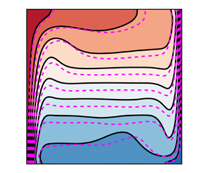
3.1. Vertical convection
3.1.1. Original equations
The flow set-up and original governing equations are completely equivalent to those used in Wang et al. (Reference Wang, Xia, Yan, Sun and Wan2019). After non-dimensionalization, the 2-D flow region is  $\mathcal {V}=[-0.5,0.5]^2$. The coordinates
  $x$ and
  $y$ are those of the horizontal and vertical directions, respectively;
  $u$ and
  $v$ are the corresponding velocity components; and
  $\lambda \in (0,1)$ characterizes the difference of temperature
  $T$ between the vertical walls. This problem can be described by (2.1a) and (2.1b), together with the following governing equation for temperature
  $T$ and a relation between
  $\rho$ and
  $T$:
$T$:
 $$\begin{gather} \frac{\partial{T}}{\partial{t}}+\boldsymbol{u}\boldsymbol{\cdot}\boldsymbol{\nabla}{T} ={-}\frac{1}{\rho c_p} \left[\boldsymbol{\nabla}\boldsymbol{\cdot}\boldsymbol{J} +\frac{\gamma-1}{V} \int_{\mathcal{V}}{\boldsymbol{\nabla}\boldsymbol{\cdot}\boldsymbol{J}\,\textrm{d}V}\right], \end{gather}$$
 $$\begin{gather}\rho=MT^{{-}1}\left(\int_{\mathcal{V}}{\frac{\textrm{d}V}{T}}\right)^{{-}1}, \end{gather}$$
as well as the boundary conditions (Wang et al. Reference Wang, Xia, Yan, Sun and Wan2019)
 $$\begin{gather} x=\pm0.5{:}\quad \boldsymbol{u}=0,\quad T=1\mp\lambda, \end{gather}$$
 $$\begin{gather}y=\pm0.5{:}\quad \boldsymbol{u}=0,\quad \partial{T}/\partial{y}=0. \end{gather}$$
 Straightforwardly, the density source term  $Q$ in (2.1c) can be derived as
 \begin{equation} \frac{\textrm{d}\rho}{\textrm{d}t}=Q =\frac{1}{T}\left(\boldsymbol{\nabla}\boldsymbol{\cdot}\boldsymbol{J} -\frac{1}{V}\int_{\mathcal{V}}{\boldsymbol{\nabla}\boldsymbol{\cdot}\boldsymbol{J}\,\textrm{d}V}\right). \end{equation}
Here the specific heat ratio  $\gamma =1.4$. The total mass
  $M$, the total volume
  $V$ and the isobaric specific heat
  $c_p$ are all assumed to be
  $1$. The body force
  $\boldsymbol {f}=-(2\lambda )^{-1}\boldsymbol {e}_y$; the viscous stress tensor and heat flux are
 \begin{equation} \boldsymbol{\mathsf{T}}=\mu[\boldsymbol{\nabla}\boldsymbol{u}+(\boldsymbol{\nabla}\boldsymbol{u})^\textrm{T} -\tfrac{2}{3}\boldsymbol{\mathsf{I}}(\boldsymbol{\nabla}\boldsymbol{\cdot}\boldsymbol{u})], \quad \boldsymbol{J}={-}\kappa\boldsymbol{\nabla} T , \end{equation}
respectively, where  $\mu$ and
  $\kappa$ follow the Sutherland laws:
 \begin{equation} \mu=\sqrt{\frac{Pr}{Ra}}\,T^{1.5}\frac{1+S_{\mu}}{T+S_{\mu}}, \quad \kappa=\sqrt{\frac{1}{RaPr}}\,T^{1.5}\frac{1+S_{\kappa}}{T+S_{\kappa}}, \end{equation}
with  $S_{\mu }=0.368$ and
  $S_{\kappa }=0.648$, and
  $Ra$ and
  $Pr$ are the Rayleigh number and Prandtl number, respectively.
The LMN equations are solved using a second-order central difference code on a uniform grid. The corresponding hydrodynamic pressure equation (2.2) is solved using the successive over-relaxation (SOR) method. Using a time-stepping approach, steady solutions  $(\bar {\boldsymbol {u}}(\boldsymbol {x}),\bar {T}(\boldsymbol {x}))$ are achieved in the sense of machine precision. The code is validated at
  $Ra=10^6$,
  $Pr=0.71$ and varying
  $\lambda$. The Oberbeck–Boussinesq (OB) approximation can be simulated in the present code with
  $\lambda \approx 0$. With increasing
  $\lambda$, the non-OB effect will emerge and it is non-negligible in the cases with
  $\lambda =0.2$, 0.4 and 0.6. The Nusselt numbers
  $Nu$ from the present simulations are compared with the reference values from Wang et al. (Reference Wang, Xia, Yan, Sun and Wan2019). As shown in table 1, the present code can accurately predict
  $Nu$ for all cases with relative deviations less than
  $0.1\,\%$, demonstrating the correctness of the present code in a wide range of
  $\lambda$.
Table 1. Comparison of Nusselt numbers  $Nu$ at
  $Ra=10^6$,
  $Pr=0.71$ and varying
  $\lambda$ from present simulations and the reference works from Wang et al. (Reference Wang, Xia, Yan, Sun and Wan2019). Note that the grid is uniform and its size is
  $256\times 256$.

Using the present code corresponding to the LMN equations,  $13$ simulations are performed on a uniform
  $256\times 256$ grid at
  $Ra=10^6$,
  $Pr=0.71$ and
  $\lambda =0.6\times (2/3)^n$ with integer
  $n$ ranging from
  $0$ to
  $12$. The
  $13$ cases are regarded as the reference cases with the steady flow fields
  $(\bar {\boldsymbol {u}}(\boldsymbol {x};\lambda ),\bar {T}(\boldsymbol {x};\lambda ))$, which will be used to assess the results corresponding to different orders of the type-II buoyancy terms.
3.1.2. Modified equations
In order to apply the type-II buoyancy terms, the modified momentum equation (2.3) is used to substitute (2.1b), while the other basic equations and parameters are kept unchanged. In addition,  $\rho _0$ is chosen as
  $M(\int _{\mathcal {V}} \textrm {d} V/T)^{-1}$, so that
  $\epsilon =\max _{\mathcal {V}}[|\rho '/\rho |]\equiv \lambda$.
Since  $\|\boldsymbol {f}\|\sim O(\epsilon ^{-1})$ and
  $\|\boldsymbol {A}+\boldsymbol {C}+\boldsymbol {D}\|\sim O(1)$, an
  $n$th-order type-II buoyancy term
  $\hat {\boldsymbol {B}}^{(n)}$ has a relative error of
  $O(\epsilon ^n)$ according to § 2.4. Clearly, the error of
  $\hat {\boldsymbol {B}}^{(n)}$ is also
  $O(\epsilon ^n)$. Four groups of steady flow fields
  $(\bar {\boldsymbol {u}}^{(n)},\bar {T}^{(n)})$ are defined corresponding to different orders of type-II buoyancy terms
  $\hat {\boldsymbol {B}}^{(n)}$, with
  $n=1,2,3,\infty$. All other flow variables have the same superscripts as the corresponding buoyancy terms.
The modified equations are solved using a finite-difference code which is almost the same as that described in § 3.1.1, except that the Poisson equations are decoupled using DCT and solved directly (Zhang & Bao Reference Zhang and Bao2015; Zhang et al. Reference Zhang, Xia, Zhou and Chen2020). The simulation results using this code and the Boussinesq approximation are compared with those in de Vahl Davis & Jones (Reference de Vahl Davis and Jones1983) or Wang et al. (Reference Wang, Xia, Yan, Sun and Wan2019) for  $Ra=10^4$,
  $10^5$,
  $10^6$ and
  $Pr=0.71$, and the relative errors are again less than
  $0.1\,\%$. Although an infinite sequence of Poisson equations is required for computing
  $\hat {\boldsymbol {B}}^{(\infty )}$ theoretically, solving
  $100$ extra Poisson equations for each time step is sufficient to make the residual converge to
  $0$ in the sense of machine precision for
  $\epsilon \leq 0.6$. Each group of flow fields described by the modified equations have the same parameters as the
  $13$ cases described in § 3.1.1, that is,
  $Ra=10^6$,
  $Pr=0.71$ and
  $\lambda =0.6\times (2/3)^n$ with integer
  $n$ ranging from
  $0$ to
  $12$.
$12$.
3.1.3. Simulation results
A further normalized temperature is defined as  $\theta =(T-1)/2\lambda$. Figure 2 shows the contours and isolines of
  $\bar {\theta }$,
  $\bar {\theta }^{(1)}$,
  $\bar {\theta }^{(2)}$ and
  $\bar {\theta }^{(3)}$, with
  $\epsilon =\lambda =0.6$ and
  $\epsilon =\lambda =0.178$. Here
  $\epsilon =0.6$ corresponds to a large density variation (
 $\max _{\mathcal {V}}[\rho ]/\min _{\mathcal {V}}[\rho ]\equiv 4$) and
  $\epsilon =0.178$ corresponds to a medium density variation (
 $\max _{\mathcal {V}}[\rho ]/\min _{\mathcal {V}}[\rho ]\equiv 1.43$). For a large density variation (
 $\epsilon =0.6$), figure 2(b) indicates that the first-order type-II buoyancy term
  $\hat {\boldsymbol {B}}^{(1)}$, which is very close to the Boussinesq gravitational buoyancy term, is a coarse approximation and could only predict qualitative properties of the steady flow. To improve the accuracy,
  $\hat {\boldsymbol {B}}^{(2)}$ with a higher order could be used, and figure 2(c) shows that the error is very small. It should be emphasized that
  $\hat {\boldsymbol {B}}^{(2)}$ only requires solving one extra Poisson equation, which is not very expensive for the present solver. For even better approximation,
  $\hat {\boldsymbol {B}}^{(3)}$ could be used (figure 2d). Fortunately, when the density variation is not too large (
 $\epsilon =0.178$), solving one extra Poisson equation seems sufficient, because the error caused by
  $\hat {\boldsymbol {B}}^{(2)}$ is already indiscernible, as indicated by figure 2(g).

Figure 2. Contours and solid isolines with isovalues  $-0.4:(0.1):0.4$ of (a,e)
  $\bar {\theta }$, (b,f)
  $\bar {\theta }^{(1)}$, (c,g)
  $\bar {\theta }^{(2)}$ and (d,h)
  $\bar {\theta }^{(3)}$. Physical parameters are
  $Ra=10^6$,
  $Pr=0.71$ and (a–d)
  $\lambda =0.6$ and (e–h)
  $\lambda =0.178$. The purple dashed lines in (b–d, f–h) are the isolines of
  $\bar {\theta }$ with the corresponding
  $\lambda$.
To show the accuracy of type-II buoyancy terms and the ‘exact’ buoyancy term in detail, the relative errors of the steady  $\bar {\boldsymbol {u}}$ and
  $\bar {\theta }$ fields corresponding to buoyancy terms
  $\hat {\boldsymbol {B}}^{(1)}$,
  $\hat {\boldsymbol {B}}^{(2)}$,
  $\hat {\boldsymbol {B}}^{(3)}$ and
  $\hat {\boldsymbol {B}}^{(\infty )}$ are shown in figure 3(a,b). It is clearly seen that the relative errors of
  $(\bar {\boldsymbol {u}}^{(1)},\bar {\theta }^{(1)})$,
  $(\bar {\boldsymbol {u}}^{(2)},\bar {\theta }^{(2)})$ and
  $(\bar {\boldsymbol {u}}^{(3)},\bar {\theta }^{(3)})$ are
  $O(\epsilon )$,
  $O(\epsilon ^2)$ and
  $O(\epsilon ^3)$, respectively. This indicates that the error of
  $(\bar {\boldsymbol {u}}^{(n)},\bar {\theta }^{(n)})$ has the same scaling as the error of
  $\hat {\boldsymbol {B}}^{(n)}$. Such a result can be explained using the vorticity equations at steady state. For
  $n\geq 1$, we define
 \begin{equation} \delta\boldsymbol{u}^{(n)}=\bar{\boldsymbol{u}}^{(n)}-\bar{\boldsymbol{u}}, \quad \delta T^{(n)}=\bar{T}^{(n)}-\bar{T}, \quad \delta\theta^{(n)}=\bar{\theta}^{(n)}-\bar{\theta}=2\epsilon\delta T^{(n)} \end{equation}
and
 \begin{equation} \boldsymbol{\varPsi}^{(n)}(\boldsymbol{u},T) =\boldsymbol{\nabla}\times\left[\boldsymbol{u}\boldsymbol{\cdot}\boldsymbol{\nabla}\boldsymbol{u} -\frac{1}{\rho(T)}\boldsymbol{\nabla}\boldsymbol{\cdot}\boldsymbol{\mathsf{T}}(\boldsymbol{u},T) -\hat{\boldsymbol{B}}^{(n)}(\boldsymbol{u},T)\right]. \end{equation}
Using the fact that  $\partial \bar {\boldsymbol {\omega }}/\partial t=0$ and
  $\partial \bar {\boldsymbol {\omega }}^{(n)}/\partial t=0$, one has
 \begin{align} &\boldsymbol{\nabla}\times\hat{\boldsymbol{B}}^{(n)}(\bar{\boldsymbol{u}},\bar{T}) -\frac{1}{\rho^2(\bar{T})}\boldsymbol{\nabla}\rho(\bar{T}) \times\boldsymbol{\nabla}\varPi(\bar{\boldsymbol{u}},\bar{T}) \nonumber\\ &\quad =\boldsymbol{\varPsi}^{(n)}(\bar{\boldsymbol{u}}+\delta\boldsymbol{u}^{(n)}, \bar{T}+\delta T^{(n)})-\boldsymbol{\varPsi}^{(n)}(\bar{\boldsymbol{u}},\bar{T}). \end{align}
Figure 3. Relative errors of steady flow fields and properties. (a) Relative errors of velocity fields. (b) Relative errors of temperature fields. (c) Relative errors of Nusselt numbers. Errors not shown in (c) are machine zero.
It seems that, with  $(\bar {\boldsymbol {u}},\bar {T})$ fixed, the leading terms of the right-hand side of (3.8) should be characterized by
  $\delta \boldsymbol {u}^{(n)}$ and
  $\delta T^{(n)}$ and their differentials. However, since
  $\boldsymbol {\nabla }\times \hat {\boldsymbol {B}}^{(n)}$ in
  $\boldsymbol {\varPsi }^{(n)}$ contains a large coefficient
  $f\sim O(\epsilon ^{-1})$, the influence of
  $\delta T^{(n)}$ on
  $\boldsymbol {\varPsi }^{(n)}$ is amplified by
  $\epsilon ^{-1}$. Therefore, the
  $O(\epsilon ^n)$ scaling of the error of
  $\hat {\boldsymbol {B}}^{(n)}$ should be inherited by
  $\delta \boldsymbol {u}^{(n)}$ and
  $\delta \theta ^{(n)}$ via the implicit equation (3.8). Figure 3(c) shows the relative errors of
  $Nu$. Different from the results of flow fields,
  $Nu^{(1)}$ and
  $Nu^{(2)}$ both have the same
  $O(\epsilon ^2)$ scaling of relative error, and
  $Nu^{(3)}$ has an
  $O(\epsilon ^4)$ scaling of relative error. The unexpected one order higher in accuracy of
  $Nu^{(1)}$ and
  $Nu^{(3)}$ is not fully understood, but is probably caused by certain symmetry of the flow field.
For the ‘exact’ buoyancy term  $\boldsymbol {B}^{{\dagger} }=\hat {\boldsymbol {B}}^{(\infty )}$ with no error theoretically, it can also be seen from figure 3(a,b) that the steady flow fields
  $(\bar {\boldsymbol {u}}^{(\infty )},\bar {T}^{(\infty )})$ are equal to
  $(\bar {\boldsymbol {u}},\bar {T})$ in the sense of machine precision. In addition, figure 3(c) shows that the relative errors of
  $Nu^{(\infty )}$ are also negligible in the sense of machine precision. From the above results, we have confirmed by numerical simulations that for
  $\epsilon \leq 0.6$(
 $\max _{\mathcal {V}}[\rho ]/\min _{\mathcal {V}}[\rho ]\leq 4$), the modified equation (2.3) with the ‘exact’ buoyancy term
  $\boldsymbol {B}^{{\dagger} }=\hat {\boldsymbol {B}}^{(\infty )}$ is equivalent to the original LMN equations.
Figure 3 further suggests the valid  $\epsilon$ range for each buoyancy term to achieve the required accuracy. For example, if the error bound is
  $1\,\%$ for both the velocity and temperature fields,
  $\hat {\boldsymbol {B}}^{(1)}$ could only be used for
  $\epsilon \leq 0.035$, while the more accurate
  $\hat {\boldsymbol {B}}^{(2)}$ could be used for
  $\epsilon \leq 0.267$(
 $\max _{\mathcal {V}}[\rho ]/\min _{\mathcal {V}}[\rho ]\leq 1.727$), and
  $\hat {\boldsymbol {B}}^{(3)}$ is valid for
  $\epsilon \leq 0.4$. Therefore, for most flows with small and medium density variation (
 $\max _{\mathcal {V}}[\rho ]/\min _{\mathcal {V}}[\rho ]\leq 1.727$),
  $\hat {\boldsymbol {B}}^{(2)}$ should be accurate enough, and it only requires solving one extra Poisson equation (see Appendix A for the detailed computation procedure of
  $\hat {\boldsymbol {B}}^{(2)}$).
3.2. Rayleigh–Taylor instability
3.2.1. Original equations
After non-dimensionalization, the 2-D flow region is  $\mathcal {V}=[-0.5,0.5]\times [-1,1]$. The coordinates
  $x$ and
  $y$ and the velocity components
  $u$ and
  $v$ are those in the horizontal and vertical directions, respectively. The Atwood number
  $A\in (0,1)$ characterizes the density ratio, and
  $\rho _H=1+A$ and
  $\rho _L=1-A$ are defined as the density of pure heavy and light fluids, respectively. The initial shape of the interface is sinusoidal, with wavelength
  $\lambda =1$, amplitude
  $a$ and characteristic thickness
  $b$. The LMN equations (2.1a)–(2.1c) could be used here with the following boundary and initial conditions (Wei & Livescu Reference Wei and Livescu2012):
 $$\begin{gather} x=\pm0.5 {:}\quad \boldsymbol{u}=0,\quad \partial{\rho}/\partial{x}=0, \end{gather}$$
 $$\begin{gather}y= \pm1{:} \quad \boldsymbol{u}=0,\quad \partial{\rho}/\partial{y}=0, \end{gather}$$
 $$\begin{gather}t=t _0{:} \quad \boldsymbol{u}=0,\quad \rho=1-A\tanh([y+a\cos(2{\rm \pi} x)]/b). \end{gather}$$
Here, the body force  $\boldsymbol{f}=(1+A^{-1})\boldsymbol{e}_y$; and the viscous stress tensor
  $\boldsymbol{\mathsf{T}}$ and density diffusion term
  $Q$ are defined as
 \begin{equation} \boldsymbol{\mathsf{T}}=\frac{\rho}{Re}\left[\boldsymbol{\nabla}\boldsymbol{u}+(\boldsymbol{\nabla}\boldsymbol{u})^\textrm{T} -\frac{2}{3}\boldsymbol{\mathsf{I}}(\boldsymbol{\nabla}\boldsymbol{\cdot}\boldsymbol{u})\right], \quad Q=\rho\boldsymbol{\nabla}\boldsymbol{\cdot}\left(\frac{1}{ReSc}\boldsymbol{\nabla}\ln\rho\right) , \end{equation}
with  $Re$ and
  $Sc$ being the Reynolds number and Schmidt number, respectively (Wei & Livescu Reference Wei and Livescu2012).
The LMN equations are solved using a second-order central difference code on an  $N_x\times N_y=512\times 1024$ uniform grid. The corresponding hydrodynamic pressure equation (2.2) is solved using the SOR method, which is the same as that used in § 3.1. Time marching is performed using the second-order explicit Adams–Bashforth method.
In order to compare with the experimental results in Waddell, Niederhaus & Jacobs (Reference Waddell, Niederhaus and Jacobs2001), a reference LMN case is simulated with parameters  $A=0.155$,
  $Re=6000$,
  $Sc=100$,
  $a=0.02$ and
  $b=0.01$. It should be emphasized that the parameters, except for the Atwood number, were not clearly presented in Waddell et al. (Reference Waddell, Niederhaus and Jacobs2001). However, many test cases with different parameters suggest that the amplitude
  $h(t)$ (defined with the largest vertical distance between two points on the interface
  $\theta =0$) is not sensitive to
  $Re$,
$Re$,  $Sc$ and
  $b$ in a reasonable range. In addition, by choosing a small
  $a=0.02$ and a proper
  $t_0=-0.232$, the
  $h(t)$ obtained from the present simulation can match well with the experimental results at
  $A=0.155$ from Waddell et al. (Reference Waddell, Niederhaus and Jacobs2001), as shown in figure 4(a). Therefore, we believe that the LMN equations can well describe the
  $A=0.155$ case considered in Waddell et al. (Reference Waddell, Niederhaus and Jacobs2001), and the numerical code is reliable. For clarity, the flow fields and
  $h(t)$ of the reference LMN case are marked with superscript ‘
 ${\dagger}$’.

Figure 4. (a) Interface fluctuation amplitudes of the LMN reference case and the experiment (Waddell et al. Reference Waddell, Niederhaus and Jacobs2001). (b) Errors of interface fluctuation amplitudes of cases with buoyancy terms.
3.2.2. Modified equations
In order to test the performance of the buoyancy terms, the modified momentum equation (2.3) is used, while other equations and basic parameters remain unchanged. Here  $\rho _0$ is chosen as
  $1$ and thus
  $\epsilon =0.183$. The buoyancy terms tested are:
 \begin{equation} \boldsymbol{B}^B=\frac{\rho'}{\rho_0}\boldsymbol{f}, \quad \boldsymbol{B}^L=\frac{\rho'}{\rho_0}(\boldsymbol{f}-\boldsymbol{u}\boldsymbol{\cdot}\boldsymbol{\nabla}\boldsymbol{u}) \quad \text{and} \quad \hat{\boldsymbol{B}}^{(n)}\quad (n=2,3). \end{equation}
Here,  $\boldsymbol {B}^B$ is the Boussinesq buoyancy term and
  $\boldsymbol {B}^L$ is the buoyancy term from Lopez et al. (Reference Lopez, Marques and Avila2013). With the modified equations, four cases corresponding to the buoyancy terms listed above are solved using a finite-difference code almost the same as that for the LMN equations, except that the Poisson equations are solved using DCT as mentioned in § 3.1.2. The computed flow fields and interface amplitudes have the same superscripts as the corresponding buoyancy terms.
3.2.3. Simulation results
Figure 4(b) shows the errors of the interface fluctuation amplitudes  $h(t)$ computed from different buoyancy terms, and figure 5 shows the normalized density
  $\theta$ fields at
  $t=1.54$. Here,
  $\theta =(\rho -1)/2A$. Figure 5(a) shows that the motions of the ascending heavy fluid (spike) and the descending light fluid (bubble) are not fully symmetric (Waddell et al. Reference Waddell, Niederhaus and Jacobs2001). It is seen that the spike front is above
  $y=0.4$ while the bubble fronts are above
  $y=-0.4$. Such asymmetry is not well predicted by the simplest buoyancy term
  $\boldsymbol {B}^B$, which can be indicated from figure 5(b), where the height of the spike front and the depth of the bubble fronts are almost the same. In addition,
  $h^B$ is larger than
  $h^{\dagger}$ at
  $t=1.54$ as shown in figure 4(b). The revised buoyancy term
  $\boldsymbol {B}^L$ with an extra term
  $-\rho '\boldsymbol {u}\boldsymbol {\cdot }\boldsymbol {\nabla }\boldsymbol {u}/\rho _0$ (Lopez et al. Reference Lopez, Marques and Avila2013) aims to reduce the error by a factor of
  $\epsilon$. However, figure 5(c) indicates that the error of
  $\theta ^L$ is in the same scale as that of
  $\theta ^B$, and the error of
  $h^L$ turns out to be even larger than the error of
  $h^B$ in the range
  $1.95< t-t_0<2.2$ (figure 4b). There are two main reasons. First, as explained in § 2.4, the non-conservative part of the convection term is contained in
  $-\rho '\boldsymbol {u}\boldsymbol {\cdot }\boldsymbol {\nabla }\boldsymbol {u}/\rho _0$ and causes an
  $O(\epsilon )$ error. Second, the buoyancy term corresponding to the large body force
  $f\sim O(\epsilon ^{-1})$ requires further approximation. Therefore, considering the small viscosity and diffusivity, a buoyancy term with much better performance than
  $\boldsymbol {B}^B$ should at least contain
  $\boldsymbol {B}_{\boldsymbol {f}}^{(2)}$ and
  $\boldsymbol {B}_{\boldsymbol {C}}^{(1)}$. The significant improvement of accuracy achieved by
  $\hat {\boldsymbol {B}}^{(2)}$ can be indicated by figure 5(d), where the difference of the interface between
  $\theta ^{(2)}$ and
  $\theta ^{\dagger}$ is hardly discernible. Clearly, the asymmetric motions of the spike and bubbles are recovered by
  $\hat {\boldsymbol {B}}^{(2)}$. This result suggests that such asymmetry is mainly caused by a part of the baroclinic torque which is neglected by the Boussinesq buoyancy term, and this part can be well described by two correction terms
  $\boldsymbol {B}_{\boldsymbol {C}}^{(1)}$ and
  $\boldsymbol {B}_{\boldsymbol {f}}^{(2)}-\rho '\boldsymbol {f}/\rho _0$. This can be useful in the theoretical analysis on baroclinic effects in Rayleigh–Taylor instability. In addition, the error of
  $h^{(2)}$ is greatly reduced as compared with that of
  $h^B$ (figure 4b), indicating that
  $\hat {\boldsymbol {B}}^{(2)}$ is a higher-order correction instead of
  $\boldsymbol {B}^L$. Figure 4(b) also shows that the error of
  $h^{(3)}$ is significantly reduced as compared with that of
  $h^{(2)}$. This supports the convergence of the modified equations (§ 3.2.2) with
  $\hat {\boldsymbol {B}}^{(n)}$ and increasing
  $n$.
$n$.

Figure 5. Contours and solid isolines with isovalue  $0$ at
  $t=1.54$ of (a)
  $\theta ^{\dagger}$, (b)
  $\theta ^B$, (c)
  $\theta ^L$ and (d)
  $\theta ^{(2)}$. The purple dashed lines in (b–d) represent the isoline of
  $\theta ^{\dagger}$. White lines denote the vertical positions of spike fronts.
4. Conclusion
In the present paper, a regular perturbation method is applied to the hydrodynamic pressure equation, leading to a sequence of Poisson equations. The solutions of the Poisson equations form a series expansion of baroclinic torque, and thus the error analysis of any buoyancy term can be performed. We examined the errors related to several existing buoyancy terms, and identified invalid buoyancy terms which may lead to wrong predictions on flow physics. New types of buoyancy terms constructed with the perturbation solutions, namely the  $n$th-order partial buoyancy terms, type-I buoyancy terms and type-II buoyancy terms, are proved to be accurate theoretically and numerically. In addition, we discussed the frame invariance of the buoyancy terms and found that the type-I buoyancy terms are invariant under classical frame transformations, while the Boussinesq gravitational buoyancy term and the type-II buoyancy terms are invariant under frame transformations between inertial frames.
Two numerical cases, static vertical convection and transient Rayleigh–Taylor instability, were simulated to examine the accuracy of our newly proposed type-II buoyancy terms. The results confirmed that the relative error of  $\hat {\boldsymbol {B}}^{(n)}$ is
  $O(\epsilon ^n)$, as expected. Furthermore, the results in Rayleigh–Taylor instability suggest that the extra contribution from
  $\hat {\boldsymbol {B}}^{(2)}$ over the Boussinesq buoyancy term is the key factor to determine the asymmetry of the evolution of the bubbles and spikes. This may help us to understand the underlying physics related to the baroclinic effect theoretically.
Finally, we would like to stress that the present type-I and type-II buoyancy terms might be useful in variable-density flow simulations where spectral Poisson solvers are used. In addition, numerical simulations indicate that for buoyancy-driven flows with small or medium density variation, the second-order type-II buoyancy term is sufficiently accurate and it only requires one extra Poisson equation to be solved.
Supplementary material
Supplementary material is available at https://doi.org/10.1017/jfm.2021.896.
Acknowledgement
The authors would like to thank Professor D. Lohse for many useful suggestions.
Funding
This work was supported by the National Science Foundation of China (NSFC grant nos 11988102, 11822208, 11772297 and 91852205) and Shenzhen Science and Technology Programme (no. KQTD20180411143441009).
Declaration of interests
The authors report no conflict of interest.
Appendix A. Numerical procedure for $\hat {\boldsymbol {B}}^{(2)}$

Following the definition (2.21), the second-order type-II buoyancy term  $\hat {\boldsymbol {B}}^{(2)}$ can be written as
 \begin{equation} \hat{\boldsymbol{B}}^{(2)}=\frac{\rho'}{\rho}\boldsymbol{f}+\frac{\epsilon\rho'}{\rho_0\rho}\boldsymbol{\nabla}\hat{\varPi}^{(1)}, \end{equation}
where  $\hat {\varPi }^{(1)}$ could be computed by solving the Poisson equation
 \begin{equation} \left. \begin{gathered} \mathcal{V}{:}\quad \nabla^2\hat{\varPi}^{(1)} =\epsilon^{{-}1}\rho_0\left[\boldsymbol{\nabla}\boldsymbol{\cdot} \left(\boldsymbol{C}+\boldsymbol{D}+\frac{\rho'}{\rho}\boldsymbol{f}\right) +\frac{\partial}{\partial{t}}\left(\frac{Q}{\rho}\right)\right],\\ \partial \mathcal{V}{:}\quad \boldsymbol{n}\boldsymbol{\cdot}\boldsymbol{\nabla}\hat{\varPi}^{(1)} =\epsilon^{{-}1}\rho_0\left[\boldsymbol{n}\boldsymbol{\cdot} \left(\boldsymbol{C}+\boldsymbol{D}+\frac{\rho'}{\rho}\boldsymbol{f}\right) +\frac{\partial(\boldsymbol{n}\boldsymbol{\cdot}\boldsymbol{u})}{\partial{t}} -\frac{\partial\boldsymbol{n}}{\partial{t}}\boldsymbol{\cdot}\boldsymbol{u}\right]. \end{gathered}\right\} \end{equation}


