2.1 Notation

Our notation is shown in the measurement volume inset in figure 1 and largely follows that of Lefauve et al. (Reference Lefauve, Partridge, Zhou, Caulfield, Dalziel and Linden2018) (hereafter LPZCDL18). The duct considered in this paper has length $L=1350~\text{mm}$ and a square cross-section of height and width $H=45~\text{mm}$ (the same dimensions as LPZCDL18 but smaller than ML14). The streamwise $x$ axis is aligned along the duct and the spanwise $y$ axis across the duct, making the $z$ axis tilted at an angle $\unicode[STIX]{x1D703}$ from the vertical (resulting in a non-zero streamwise projection of gravity $g\sin \unicode[STIX]{x1D703}$ ). All coordinates are centred in the middle of the duct, such that $-L/2\leqslant x\leqslant L/2$ and $-H/2\leqslant y,z\leqslant H/2$ . The velocity vector field has components $\boldsymbol{u}(x,y,z,t)=(u,v,w)$ along $x,y,z$ , and we denote the density field by $\unicode[STIX]{x1D70C}(x,y,z,t)$ .

The parameters believed to play important roles are the geometrical parameters: $L$ , $H$ , $\unicode[STIX]{x1D703}$ and the dynamical parameters: the reduced gravity $g^{\prime }\equiv g\unicode[STIX]{x0394}\unicode[STIX]{x1D70C}/\unicode[STIX]{x1D70C}_{0}$ (under the Boussinesq approximation of small density differences $0<\unicode[STIX]{x0394}\unicode[STIX]{x1D70C}/\unicode[STIX]{x1D70C}_{0}\ll 1$ ), the kinematic viscosity of water $\unicode[STIX]{x1D708}=1.05\times 10^{-6}~\text{m}^{2}~\text{s}^{-1}$ and the molecular diffusivity of salt $\unicode[STIX]{x1D705}_{s}=1.50\times 10^{-9}~\text{m}^{2}~\text{s}^{-1}$ . The last important parameter is the scale of the streamwise velocity $\unicode[STIX]{x0394}U$ , but it is not independent from the previous six parameters as we discuss in § 2.2. From these seven parameters having two dimensions (of length and time), we construct five independent non-dimensional parameters in § 2.3.

2.2 Scaling of the velocity

Meyer & Linden (Reference Meyer and Linden2014) recognised that the two-layer exchange flow in the SID is maximal because it is hydraulically controlled at both ends of the duct where it meets the reservoirs through a sharp change in geometry (an idea already present in Wilkinson (Reference Wilkinson1986)). In other words, the flow is subcritical with respect to long interfacial waves inside the duct (information propagates in both directions), and critical at either end, preventing the propagation of information (in particular of the exchange flow rate) from the exterior into the interior of the duct. The resulting flow is therefore said to be controlled by the interior and maximal in the sense that it has the largest exchange flow rate of any realisable flow (for more details, see ML14, Lefauve et al. Reference Lefauve, Partridge, Zhou, Caulfield, Dalziel and Linden2018, § 3, and Lefauve Reference Lefauve2018, § 1.3.2). This maximal exchange flow is sustained in a quasi-steady state until the controls are ‘flooded’ by the accumulation of fluid of a different density coming from the other reservoir. With each reservoir holding approximately 100 litres of fluid in our current set-up, a typical experiment can last several minutes, which represents many duct transit times (streamwise advection time along the length of the duct).

As a consequence, the velocity scale $\unicode[STIX]{x0394}U$ is not an independent parameter; it is set by the phase speed of long interfacial gravity waves. To understand this, we follow the literature (see e.g. Armi (Reference Armi1986), Lawrence (Reference Lawrence1990)) and consider the composite Froude number of this two-layer flow as

(2.1) $$\begin{eqnarray}\displaystyle G^{2}(x)\equiv F_{1}^{2}(x)+F_{2}^{2}(x),\quad \text{where}~F_{i}^{2}(x)\equiv {\displaystyle \frac{\langle u_{i}^{2}(x)\rangle _{y,z_{i}}}{g^{\prime }h_{i}(x)}} & & \displaystyle\end{eqnarray}$$

is the Froude number of layer $i$ , $\langle \cdot \rangle _{y,z_{i}}$ denotes spanwise and vertical averaging over the depth $h_{i}$ of each layer and the symbol $\equiv$ denotes a definition. In the idealised case of frictionless, horizontal ducts ( $\unicode[STIX]{x1D703}=0^{\circ }$ ), the flow is streamwise invariant and $G$ takes everywhere the value at the centre of the duct

(2.2) $$\begin{eqnarray}\displaystyle G(x)=G(0)=2{\displaystyle \frac{\langle |u|\rangle _{y,z}}{\sqrt{g^{\prime }H}}}, & & \displaystyle\end{eqnarray}$$

where $\langle \cdot \rangle _{y,z}$ denotes averaging over the whole duct cross-section. The second equality results from (2.1) and the symmetry of the flow at $x=0$ guaranteed by the Boussinesq approximation ( $\langle |u_{1}|\rangle _{y,z}=\langle |u_{2}|\rangle _{y,z}$ and $h_{1}=h_{2}=H/2$ ). Note that here and in the remainder of the paper, we assume that the exchange flow has zero net (or ‘barotropic’) flow rate $\langle u\rangle _{y,z}=0$ , which is a good approximation in the present set-up. Hydraulic control requires that $G^{2}=1$ (Armi Reference Armi1986), which gives the following layer-averaged velocity

(2.3) $$\begin{eqnarray}\displaystyle \langle |u|\rangle _{y,z}={\displaystyle \frac{\sqrt{g^{\prime }H}}{2}}, & & \displaystyle\end{eqnarray}$$

as previously recognised by ML14. With the addition of viscous friction and/or of a non-zero tilt angle, the flow is no longer streamwise invariant: $G(x)$ is maximal at the ends ( $x=\pm L/2$ ) and minimal in the centre ( $x=0$ ). Since the criticality condition $G^{2}=1$ is imposed at the ends where the controls occur $G(\pm L/2)=1>G(0)$ , the velocity scale $\langle |u|\rangle _{y,z}=(\sqrt{g^{\prime }H}/2)G(0)$ is lower than the inviscid upper bound (2.3) that we call the ‘hydraulic limit’ (see Gu & Lawrence (Reference Gu and Lawrence2005) for more details). As first observed in ML14 (see their figure 7) and as we shall substantiate in § 4.3.1, this hydraulic limit is however generally achieved when a positive tilt angle $\unicode[STIX]{x1D703}>0^{\circ }$ is added to counterbalance the dissipative effects of viscosity.

Due to the moderate Reynolds numbers and the long duct investigated in the present set-up, the velocity profiles are usually significantly affected by viscosity in the sense that viscous boundary layers at the walls and interface are partially or fully developed. Generally, we find that the peak velocities in each layer are at most around twice the layer-averaged values corresponding to the hydraulic limit (2.3), i.e.  $\max _{y,z}|u|\approx 2\langle |u|\rangle _{y,z}\approx \sqrt{g^{\prime }H}$ . We therefore choose to non-dimensionalise velocities by this characteristic ‘peak’ value, i.e. half the total (peak-to-peak) velocity jump (shown in the inset in figure 1):

(2.4) $$\begin{eqnarray}\displaystyle {\displaystyle \frac{\unicode[STIX]{x0394}U}{2}}\equiv \sqrt{g^{\prime }H}. & & \displaystyle\end{eqnarray}$$

2.3 Non-dimensionalisation

Based on the above, we define the non-dimensional velocity vector as $\tilde{\boldsymbol{u}}\equiv \boldsymbol{u}/(\unicode[STIX]{x0394}U/2)$ such that in general $-1\lesssim \tilde{u} \lesssim 1$ (noting that the streamwise velocity is dominant in this flow, i.e.  $|\tilde{u} |\gg |\tilde{v}|,|\tilde{w}|$ ). For consistency, we choose $H/2$ as the length scale, defining the non-dimensional position vector as $\tilde{\boldsymbol{x}}\equiv \boldsymbol{x}/(H/2)$ such that $-1\leqslant {\tilde{y}},\tilde{z}\leqslant 1$ , and $-A\leqslant \tilde{x}\leqslant A$ , where the aspect ratio of the duct is

(2.5) $$\begin{eqnarray}\displaystyle A\equiv {\displaystyle \frac{L}{H}}. & & \displaystyle\end{eqnarray}$$

Consequently, we non-dimensionalise time by the advective time unit $H/\unicode[STIX]{x0394}U=1/(2\sqrt{g^{\prime }/H})$ : $\tilde{t}\equiv 2\sqrt{g^{\prime }/H}t$ (hereafter abbreviated ATU). The dimensionless density field is defined as $\tilde{\unicode[STIX]{x1D70C}}\equiv (\unicode[STIX]{x1D70C}-\unicode[STIX]{x1D70C}_{0})/(\unicode[STIX]{x0394}\unicode[STIX]{x1D70C}/2)$ , such that $-1\leqslant \tilde{\unicode[STIX]{x1D70C}}\leqslant 1$ .

Using the previously defined velocity and length scales, we construct the Reynolds number

(2.6) $$\begin{eqnarray}\displaystyle Re\equiv {\displaystyle \frac{{\displaystyle \frac{\unicode[STIX]{x0394}U}{2}}{\displaystyle \frac{H}{2}}}{\unicode[STIX]{x1D708}}}={\displaystyle \frac{\sqrt{g^{\prime }H}H}{2\unicode[STIX]{x1D708}}}=1.42\times 10^{4}\,\sqrt{{\displaystyle \frac{\unicode[STIX]{x0394}\unicode[STIX]{x1D70C}}{\unicode[STIX]{x1D70C}_{0}}}}, & & \displaystyle\end{eqnarray}$$

where the last equality shows that $Re$ is a function of the driving density difference $\unicode[STIX]{x0394}\unicode[STIX]{x1D70C}/\unicode[STIX]{x1D70C}_{0}$ alone (the prefactor only holds for aqueous salt solutions in the geometry investigated here). In this paper, we present experiments in the range $\unicode[STIX]{x0394}\unicode[STIX]{x1D70C}/\unicode[STIX]{x1D70C}_{0}\in [5\times 10^{-4},1.3\times 10^{-1}]$ , i.e.  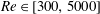$Re\in [300,5000]$ .

The velocity scale $\unicode[STIX]{x0394}U$ leads to the definition of an overall bulk Richardson number $Ri_{B}$ , expressed as the non-dimensional product of the density, length and inverse square velocity scales, and which here takes a constant value

(2.7) $$\begin{eqnarray}\displaystyle Ri_{B}\equiv {\displaystyle \frac{{\displaystyle \frac{g}{\unicode[STIX]{x1D70C}_{0}}}{\displaystyle \frac{\unicode[STIX]{x0394}\unicode[STIX]{x1D70C}}{2}}{\displaystyle \frac{H}{2}}}{\left({\displaystyle \frac{\unicode[STIX]{x0394}U}{2}}\right)^{2}}}={\displaystyle \frac{1}{4}}, & & \displaystyle\end{eqnarray}$$

by criticality of the exchange flow and our definition of $\unicode[STIX]{x0394}U$ in (2.4).

Our last non-dimensional parameter is the Schmidt number, the ratio of the momentum to salt diffusivity

(2.8) $$\begin{eqnarray}\displaystyle Sc\equiv {\displaystyle \frac{\unicode[STIX]{x1D708}}{\unicode[STIX]{x1D705}_{s}}}. & & \displaystyle\end{eqnarray}$$

In summary, we have a total of four free independent non-dimensional input parameters: $\unicode[STIX]{x1D703}$ , $A$ , $Re$ , $Sc$ , and one imposed parameter $Ri_{B}$ . For the apparatus considered, we have $A=30$ , $Sc=700$ , $Ri_{B}=1/4$ , and we have the freedom to vary $\unicode[STIX]{x1D703}$ and $Re$ (by varying $\unicode[STIX]{x0394}\unicode[STIX]{x1D70C}/\unicode[STIX]{x1D70C}_{0}$ ), allowing us to access all flow regimes.

Henceforth, we drop the tildes and, unless explicitly stated otherwise, use non-dimensional variables throughout.

2.4 Previous studies

Meyer & Linden (Reference Meyer and Linden2014) (ML14) mapped the distribution of the four regimes described in § 1 in the $\unicode[STIX]{x1D703}-\unicode[STIX]{x0394}\unicode[STIX]{x1D70C}/(2\unicode[STIX]{x1D70C}_{0})$ plane for 93 experiments (see their figure 5). They sought an equation for the transition curves by arguing that, because of the presence of hydraulic controls (§ 2.2), the kinetic energy in the flow was bounded by the scaling $(\unicode[STIX]{x0394}U)^{2}\sim g^{\prime }H$ (see (2.3) and (2.4)) and thus it could not increase even in the presence of gravitational forcing when $\unicode[STIX]{x1D703}>0^{\circ }$ . The dimensional ‘excess kinetic energy’ $g^{\prime }L\sin \unicode[STIX]{x1D703}$ , gained by conversion from potential energy by the fluid travelling a distance $L$ along the duct in the streamwise field of gravity $g^{\prime }\sin \unicode[STIX]{x1D703}>0$ , thus has to be dissipated by increased wave activity or turbulence. They non-dimensionalised this excess kinetic energy by $(\unicode[STIX]{x1D708}/H)^{2}$ , thus forming the following Grashof number

(2.9) $$\begin{eqnarray}\displaystyle Gr\equiv {\displaystyle \frac{g^{\prime }L\sin \unicode[STIX]{x1D703}}{(\unicode[STIX]{x1D708}/H)^{2}}}=4A\sin \unicode[STIX]{x1D703}Re^{2}, & & \displaystyle\end{eqnarray}$$

where the first equality is their definition and the second equality uses our notation. They found reasonable agreement between this scaling in $\sin \unicode[STIX]{x1D703}Re^{2}$ (using two different aspect ratios $A=15,\,30$ ) and suggested the empirical equation $Gr=4\times 10^{7}$ for the $\mathsf{I}\rightarrow \mathsf{T}$ transition curve (see their figure 8). The limitations of this proposed $Gr$ scaling will be discussed in § 2.5.

Macagno & Rouse (Reference Macagno and Rouse1961) (MR61) is the first study of the SID we are aware of. They mapped the same four regimes independently rediscovered by ML14 in a two-dimensional space (see their figure 8), but instead of using the two natural input parameters $\unicode[STIX]{x1D703}$ and $Re$ emerging from the above dimensional analysis, they used a Froude number and a Reynolds number based on measured values of the actual (output) $\unicode[STIX]{x0394}U$ and of the vertical distance between the two maxima of $|u|$ (depth of the shear layer). They varied $\unicode[STIX]{x1D703}$ in non-trivial ways, sometimes during an experiment, in order to obtain target values of $\unicode[STIX]{x0394}U$ and therefore better control their Reynolds number, and did not appear to realise the presence and importance of hydraulic controls (in fact, they may have disturbed them by their use of splitter plates at the ends of the duct). The main limitation of MR61 is that they did not recognise the importance of $\unicode[STIX]{x1D703}$ in the regime transitions, and were thus unable to propose a convincing physical model to substantiate them.

Kiel (Reference Kiel1991) (K91) proposed a heuristic scaling based on a ‘geometric Richardson number’ $Ri_{G}$ , whose inverse (using our notation)

(2.10) $$\begin{eqnarray}\displaystyle Ri_{G}^{-1}\equiv 4A\tan \unicode[STIX]{x1D703}+{\textstyle \frac{16}{9}} & & \displaystyle\end{eqnarray}$$

can be interpreted as the non-dimensionalisation of the ‘excess kinetic energy’ $g^{\prime }L\sin \unicode[STIX]{x1D703}$ of ML14 by the actual kinetic energy of the hydraulically controlled flow $(\unicode[STIX]{x0394}U)^{2}=g^{\prime }H$ , i.e.  $Ri_{G}^{-1}\sim g^{\prime }L\sin \unicode[STIX]{x1D703}/(g^{\prime }H)=A\sin \unicode[STIX]{x1D703}$ (disregarding constants). He argued that transition to turbulence occurs when the excess energy to be dissipated becomes large compared to the maximum kinetic energy of the flow (high $Ri_{G}^{-1}$ ). The main limitation of K91 in the context of the present study is that he intentionally focused on large $Re$ and assumed that viscous effects could be ignored. Although K91 did use large $Re$ (of order $10^{4}$ ) using ducts of dimensions similar to that of ML14, the observations of ML14 at similar $Re$ highlight the importance of $Re$ in the scaling, which we substantiate in this paper. Consequently, this $Ri_{G}$ criterion is not sufficient to explain regime transitions.

2.5 Observed regime transitions and motivation

To further motivate the need to revisit the problem of regime transitions, we reproduced the regime diagram of ML14 in a slightly different duct geometry in figure 2. The duct used in this paper had a smaller cross-section than that used by ML14 ( $H=45~\text{mm}$ versus $100~\text{mm}$ ), but had the same aspect ratio $A=30$ as that used by ML14 to obtain most of their data. We visually identified the four regimes $\mathsf{L},\mathsf{H},\mathsf{I},\mathsf{T}$  for a total of 360 experiments corresponding to different $(\unicode[STIX]{x1D703},Re)$ couples. Out of these, 312 data points come from shadowgraph observations (as in ML14), 35 come from the volumetric measurements of density and velocity described in § 3 and 13 come from simpler planar measurements that were carried out before the volumetric system was operational (these measurements are not discussed in this paper).

Figure 2. Regime diagram in the $(\unicode[STIX]{x1D703},Re)$ plane of non-dimensional input parameters totalling 360 data points (most were determined from shadowgraph observations). In dashed, the $\mathsf{I}\rightarrow \mathsf{T}$ transition curve inferred by ML14 from their experiments in a larger duct.

We observe that the regimes largely occupy distinct regions of the $\unicode[STIX]{x1D703}-Re$ plane with clear boundaries that are simple open curves, which we refer to as the $\mathsf{L}\rightarrow \mathsf{H}$ , $\mathsf{H}\rightarrow \mathsf{I}$ , and $\mathsf{I}\rightarrow \mathsf{T}$ transitions. To fix ideas, we may formally define a ‘regime function’ $\text{reg}$ taking arbitrary but increasing values such as

(2.11a-d ) $$\begin{eqnarray}\displaystyle \text{reg}\equiv 1\text{ for }\mathsf{L},\quad 2\text{ for }\mathsf{H},\quad 3\text{ for }\mathsf{I},\quad 4\text{ for }\mathsf{T}. & & \displaystyle\end{eqnarray}$$

Finding the scaling of regime transitions is equivalent to finding the functional dependence of $\text{reg}(\unicode[STIX]{x1D703},Re)$ , with ‘transition curves’ being described, for example, by the equations $\text{reg}=1.5,2.5,3.5$ . Although sufficiently far from the transition curves, the flow regime is repeatable for a given $(\unicode[STIX]{x1D703},Re)$ , we observe a slight overlap between regimes near the transitions which could be explained by two potential reasons:

(i) the flow regime may not be a reproducible characteristic of the experiment (and of the underlying dynamical system) near the transitions due to its sensitivity to flow parameters, and/or to initial conditions (the initial transients resulting from the way the experiment is started, which cannot be controlled accurately);

(ii) the qualitative (visual) identification of flow regimes, i.e. the very definition of ‘flow regime’, is not appropriate near the transitions (i.e. not fine or consistent enough) to classify the flow into the four discrete categories of ML14.

Note that throughout this paper, we use the term transition to refer to the change in the qualitative long-term (asymptotic) dynamics of the flow caused by changes in the input parameters. Although mathematically such behaviour is typically referred to as a bifurcation, we chose to avoid this term in this paper since we do not prove nor imply that the underlying dynamical system indeed exhibits strict bifurcations. This question is interesting but outside the scope of this paper.

The $\mathsf{I}\rightarrow \mathsf{T}$ transition curve proposed by ML14 (see § 2.4) is reproduced in dashed black in figure 2 to highlight the fact that the agreement in our geometry (smaller duct) is less convincing. The ML14 curve lies entirely in the $\mathsf{T}$  region (i.e. it is ‘too high’) and the discrepancy is particularly apparent at higher angles $\unicode[STIX]{x1D703}\gtrsim 4^{\circ }$ (which were not considered by ML14), suggesting that their proposed $Gr\sim \sin \unicode[STIX]{x1D703}Re^{2}$ scaling may not be universal.

To summarise, we have seen that regime transitions in the SID depend on at least two input parameters: $\unicode[STIX]{x1D703}$ and $Re$ . The first two attempts to understand the transitions (MR61 and K91) each ignored one of them, proposing heuristic scalings based on (respectively) either $Re$ or $\unicode[STIX]{x1D703}$ . More recently, ML14 correctly identified the $\unicode[STIX]{x1D703}-Re$ dependence, understood the role of hydraulic controls and proposed a transition scaling following $Gr\sim \sin \unicode[STIX]{x1D703}Re^{2}=\text{const.}$ (see (2.9)). This scaling was based on physical arguments of excess kinetic energy, which, as we will show in this paper, are essentially correct but will be made more specific. However, the first limitation of this $Gr$ criterion is that the non-dimensionalisation of the excess kinetic energy by the square velocity scale $(\unicode[STIX]{x1D708}/H)^{2}$ leading to the Grashof number $Gr$ is not justifiable by physical principles, and subsequently nor is the value $Gr=4\times 10^{7}$ for the $\mathsf{I}\rightarrow \mathsf{T}$ transition. The second limitation of the $Gr$ criterion is that it does not appear to agree with our more recent and comprehensive data obtained in a smaller duct (figure 2).

We believe that these limitations motivate the need for a revised scaling of regime transitions of the form $\text{reg}(\unicode[STIX]{x1D703},Re)=\text{const.}$ verified by quantitative experimental data and based on sound physical principles.

In the next two sections we introduce the experimental measurements (§ 3) and physical model (§ 4) employed to achieve this aim.

3.1 Three-dimensional, three-component (3D-3C) measurements

To provide a quantitative basis to the qualitative shadowgraph observations and subsequent categorisation into flow regimes, we investigate in this paper the detailed energetics underpinning each regime. To do so, we employed simultaneous measurements of the density field and three-dimensional, three-component (3D-3C) velocity field in a volume, as sketched in the inset of figure 1.

These measurements relied on a novel technique introduced by Partridge, Lefauve & Dalziel (Reference Partridge, Lefauve and Dalziel2019) in which a thin, pulsed vertical laser sheet (in the $x{-}z$ plane) is scanned rapidly back and forth in the spanwise direction (along $y$ ) to span a duct sub-volume of non-dimensional cross-section $2\times 2$ and non-dimensional length $\ell$ (typically a small fraction of full duct length $\ell \ll 2A$ ). Simultaneous stereo particle image velocimetry (sPIV) and planar laser induced fluorescence (PLIF) are employed to obtain the three-dimensional, three-component velocity and density fields $(u,v,w,\unicode[STIX]{x1D70C})(x,y_{i},z,t_{i})$ in successive $x{-}z$ planes at spanwise locations $y=y_{i}$ and respective times $t=t_{i}$ . Three-dimensional volumes containing $n_{y}$ planes (i.e.  $i=1,2,\ldots ,n_{y}$ ) are then reconstructed from these plane measurements. These volumetric 3D-3C measurements are only near instantaneous in the sense that each plane $(x,y_{i},z,t_{i})$ is separated from the previous one by a small time increment $\unicode[STIX]{x1D6FF}t\equiv t_{i}-t_{i-1}$ , resulting in each volume being constructed over a non-dimensional time $\unicode[STIX]{x0394}t\equiv n_{y}\unicode[STIX]{x1D6FF}t$ . The experimental protocol and details to obtain the measurements used in this paper are identical to those discussed in LPZCDL18 §§ 3.3–3.4, who first used this novel technique to investigate the structure of Holmboe waves found in the $\mathsf{H}$ regime.

This technique provides high-resolution measurements of $(u,v,w,\unicode[STIX]{x1D70C})(x,y,z,t)$ with a typical number of data points in each coordinate $(n_{x},n_{y},n_{z},n_{t})\approx (500,30,100,300)$ per experiment (after processing 150 GB of raw data). The details of the volume location $\bar{x}$ , length $\ell$ , duration of an experiment $\unicode[STIX]{x1D70F}$ , and resolution $(\unicode[STIX]{x0394}x,\unicode[STIX]{x0394}y,\unicode[STIX]{x0394}z,\unicode[STIX]{x0394}t)\equiv (\ell /n_{x},2/n_{y},2/n_{z},\unicode[STIX]{x1D70F}/n_{t})$ for all 3D-3C experiments discussed in this paper will be given in § 5 (table 2). We discuss the physical constraints setting bounds on all of the above resolutions in appendix A.

Finally, we enforced incompressibility in all 3D-3C velocity fields by imposing $\unicode[STIX]{x1D735}\boldsymbol{\cdot }\boldsymbol{u}=0$ for each of the $n_{t}$ volumes. We employed the recent weighted divergence correction scheme of Wang et al. (Reference Wang, Gao, Wei, Li and Wang2017), which constitutes an improved and much faster variant of the general algorithm of de Silva, Philip & Marusic (Reference de Silva, Philip and Marusic2013). Encouragingly, we found that the level of correction needed (the volume-averaged relative $L^{2}$ distance between the original and corrected fields) was typically small (at most a few per cent).

3.2 Visualisations

Figure 3. Comparative visualisations of a typical (a–f) $\mathsf{L}$ flow ( $\unicode[STIX]{x1D703}=2^{\circ }$ , $Re=398$ ) and (g–l) $\mathsf{H}$ flow ( $\unicode[STIX]{x1D703}=1^{\circ }$ , $Re=1455$ ). The $\mathsf{I}$ and $\mathsf{T}$ regimes are shown in figure 4. The $\mathsf{L}$ and $\mathsf{H}$ data correspond respectively to experiments L1 and H1 listed in table 2 (discussed later). For each experiment, we plot the density field $\unicode[STIX]{x1D70C}$ and streamwise velocity field $u$ in (a,c,g,i) the vertical mid-plane of the volume $y=0$ , and in (b,d,h,j) the arbitrary cross-sectional plane $x=-14$ , all for a single arbitrary temporal snapshot: $t=150$ in (a–d), and $t=261$ in (g–j). Colour bars are identical for all plots showing density or velocity and are thus not repeated. Dotted vertical lines in the $y=0$ plane (a,c,g,i) indicate the location of the $x=-14$ plane in (b,d,h,j) and conversely. White arrows indicate the direction of the flow in each layer (in agreement with the notation of § 2.1 and figure 1). In addition, we plot for each experiment: (e,k) the temporal evolution of the volume flux $Q(t)$ and mass flux $Q_{m}(t)$ (the dashed line is the hydraulic limit $Q=0.5$ ); and (f,l) the mean vertical density, streamwise velocity and gradient Richardson number profiles (the dot symbols indicate the vertical resolution of the data).

Figure 4. Comparative visualisations of a typical (a–f) $\mathsf{I}$ flow ( $\unicode[STIX]{x1D703}=6^{\circ }$ , $Re=777$ ) and (g–l) $\mathsf{T}$ flow ( $\unicode[STIX]{x1D703}=6^{\circ }$ , $Re=1256$ ), corresponding respectively to experiments I4 and T2 of table 2 (discussed later). The legend is identical to that of figure 3, except for the temporal snapshots used here: $t=55$ in (a–d) and $t=168$ in (g–j).

Using the measurements described above, we show visualisations of a flow representative of each of the four regimes in figure 3 ( $\mathsf{L}$ and $\mathsf{H}$ regimes) and figure 4 ( $\mathsf{I}$ and $\mathsf{T}$ regimes). We compare side-by-side the same three types of data:

1. (i) an instantaneous snapshot of the density field $\unicode[STIX]{x1D70C}$ and streamwise velocity field $u$ in the vertical mid-plane $y=0$ of the measurement volume (panels a,c,g,i), and in the arbitrary cross-sectional plane $x=-14$ (panels b,d,h,j);

2. (ii) the averaged vertical density profile $\langle \unicode[STIX]{x1D70C}\rangle _{x,y,t}(z)$ , velocity profile $\langle u\rangle _{x,y,t}(z)$ , and corresponding gradient Richardson number (panels f,l) defined as

   (3.1) $$\begin{eqnarray}\displaystyle Ri_{g}(z)\equiv -Ri_{B}{\displaystyle \frac{\unicode[STIX]{x2202}_{z}\langle \unicode[STIX]{x1D70C}\rangle _{x,y,t}}{(\unicode[STIX]{x2202}_{z}\langle u\rangle _{x,y,t})^{2}}}; & & \displaystyle\end{eqnarray}$$

3. (iii) the time series of the volume flux $Q(t)$ and mass flux $Q_{m}(t)$ (panels e,k) defined respectively as the exchange volume flow rate

   (3.2) $$\begin{eqnarray}\displaystyle Q(t)\equiv \langle |u|\rangle _{x,y,z}, & & \displaystyle\end{eqnarray}$$
   and the exchange mass flow rate
   (3.3) $$\begin{eqnarray}\displaystyle Q_{m}(t)\equiv \langle \unicode[STIX]{x1D70C}u\rangle _{x,y,z}. & & \displaystyle\end{eqnarray}$$

Note that $Q_{m}=Q$ in the absence of mixing (since in this case $\unicode[STIX]{x1D70C}=\text{sgn}(u)$ ), but in general $0<Q_{m}<Q$ in the presence of mixing. The non-dimensional hydraulic limit for the volume flux set by the maximal exchange flow condition is $Q=0.5$ , such that in general $0<Q_{m}\leqslant Q\leqslant 0.5$ (the first two inequalities always hold by definition whereas the last inequality is the hydraulic limit that does not precisely hold in the experiments).

We observe that the $\mathsf{L}$ and $\mathsf{H}$ flows have a sharp density interface with a tanh-like vertical profile (figure 3 a,b,f,g,h,l), while the $\mathsf{I}$ and $\mathsf{T}$ flows have a mixing layer (figure 4 a,b,f,g,h,l), i.e. a central layer in which the vertical density gradient is smaller than the values immediately above and below it as a result of turbulent mixing across the interface. As a result, in $\mathsf{L}$ and $\mathsf{H}$ flows, the gradient Richardson number (figure 3 l) exhibits a local maximum at the density interface and two minima on either side of order $Ri_{g}\approx 0.25$ ( $\mathsf{L}$ flow) and $Ri_{g}\approx 0.15-0.20$ ( $\mathsf{H}$ flow). In the $\mathsf{I}$ flow, the local maximum at the interface largely disappears (figure 4 l), where $Ri_{g}$ is relatively constant across the shear layer and $Ri_{g}\approx 0.05-0.30$ . In the $\mathsf{T}$ flow, $Ri_{g}$ is very nearly constant throughout the shear layer at $Ri_{g}\approx 0.15$ , in good agreement with the self-adjusting arguments of an ‘equilibrium Richardson number’ (Turner Reference Turner1973, § 10.2) and of ‘marginal instability’ (Thorpe & Liu Reference Thorpe and Liu2009; Smyth & Moum Reference Smyth and Moum2013).

In the $\mathsf{L}$ and $\mathsf{H}$ regimes, the streamwise velocity profile has a sine-like vertical structure (figure 3 f,l) indicative of fully developed velocity boundary layers (expected when $Re\lesssim 50A=1500$ , the criterion for overlapping of the interfacial, top and bottom wall 99 % boundary layers at $x=0$ ). By contrast, in the $\mathsf{I}$ and $\mathsf{T}$ regimes, interfacial turbulence creates a region of approximately constant velocity gradient across the mixing layer and ‘pointier’ velocity maxima that are pushed closer to the top and bottom walls (figure 4 f,l) especially when turbulence is more intense and sustained in the $\mathsf{T}$ flow. In all regimes, these velocity maxima $\unicode[STIX]{x2202}_{z}\langle u\rangle _{x,y,t}=0$ at $|z|\approx 0.5-0.7$ caused by the no-slip condition at $z=\pm 1$ and the influence of viscosity account for the two symmetric peaks of $Ri_{g}$ .

We also note that the $\mathsf{L}$ flow is largely (i) parallel, i.e. independent of the streamwise direction $x$ , except for a very slight downward slope of the interface typical of such flows (discussed later in § 4.3.1); (ii) steady in time; (iii) symmetric about the $y=0$ and $z=0$ planes. By contrast, the $\mathsf{H}$ flow breaks the $x$ - and $t$ -invariance with a set of travelling, symmetric Holmboe waves distorting the density and velocity interfaces in a characteristic ‘cusp’-like pattern and in a quasi-periodic fashion (these ‘confined Holmboe waves’ were the focus of LPZCDL18). In addition, complex three-dimensional wave motions in the velocity field start breaking the $y=0$ and $z=0$ symmetries (figure 3 i,j).

In the $\mathsf{I}$ and $\mathsf{T}$ flows, the departure from both the $x,t$ invariances and the $y,z=0$ symmetries at any instant in time is even greater, owing to large, three-dimensional turbulent fluctuations (figure 4). Based on the amplitude and spatial scales of the fluctuations in the position of the density and velocity interfaces, and the amplitude of the temporal fluctuations in the $Q(t)$ and $Q_{m}(t)$ time series, it is tempting to classify the $\mathsf{L}$ and $\mathsf{H}$ flows in one group based on their similarity, and the $\mathsf{I}$ and $\mathsf{T}$ regimes in a different group. The $\mathsf{L}-\mathsf{H}$ flows have lower volume and mass flux, which are equal in the absence of mixing ( $Q_{m}\approx Q\approx 0.2-0.3$ ), while the $\mathsf{I}-\mathsf{T}$ flows have higher fluxes and significant mixing ( $Q_{m}\approx 0.4-0.5<Q\approx 0.5-0.6$ , close to the hydraulic limit).

Table 1. Basic characteristics of flow regimes inferred from figures 3–4. Symbol ${\sim}$ indicates a relatively small effect.

Large temporal fluctuations in both $Q$ and $Q_{m}$ are observed in the $\mathsf{I}$ and $\mathsf{T}$ regimes, but $\mathsf{I}$ flows tend to exhibit a component with longer pseudo-period associated with oscillations between laminar and turbulent events (sometimes in a quasi-periodic fashion with period $O$ (100 ATU)). This is visible in the $\mathsf{I}$ flow here (figure 4 e): the start of a turbulent event (shown here in the snapshots figure 4 a–d at $t=55$ ) follows the instability of an accelerating, largely laminar, three-layer flow. A peak in the volume flux at $t\approx 10$ triggered large-amplitude waves at both density interfaces which started overturning at $t\approx 40$ and initiated a turbulent event slowing down the flow (decreasing $Q$ and $Q_{m}$ ). Relaminarisation followed at $t\approx 130$ (increasing $Q$ and $Q_{m}$ ), and another cycle started (note that only one cycle was recorded here).

The basic characteristics of flow regimes described above are summarised in table 1.

In the next section, we introduce the mathematical framework suited to analyse the above 3D-3C measurements and understand the energetics of SID flows.

4.1 Local energy budgets

The governing equations on which all subsequent analyses are based are the incompressible Navier–Stokes equation under the Boussinesq approximation coupled to the advection–diffusion of density. Under the notation and conventions adopted in §§ 2.1–2.3, they take the following non-dimensional form:

(4.1a ) $$\begin{eqnarray}\displaystyle & \displaystyle \unicode[STIX]{x1D735}\boldsymbol{\cdot }\boldsymbol{u}=0, & \displaystyle\end{eqnarray}$$

(4.1b ) $$\begin{eqnarray}\displaystyle & \displaystyle \unicode[STIX]{x2202}_{t}\boldsymbol{u}+\boldsymbol{u}\boldsymbol{\cdot }\unicode[STIX]{x1D735}\boldsymbol{u}=-\unicode[STIX]{x1D735}p+Ri_{B}\,(-\cos \unicode[STIX]{x1D703}\,\hat{\boldsymbol{z}}+\sin \unicode[STIX]{x1D703}\,\hat{\boldsymbol{x}})\unicode[STIX]{x1D70C}+{\displaystyle \frac{1}{Re}}\unicode[STIX]{x1D6FB}^{2}\boldsymbol{u}, & \displaystyle\end{eqnarray}$$

(4.1c ) $$\begin{eqnarray}\displaystyle & \displaystyle \unicode[STIX]{x2202}_{t}\unicode[STIX]{x1D70C}+\boldsymbol{u}\boldsymbol{\cdot }\unicode[STIX]{x1D735}\unicode[STIX]{x1D70C}={\displaystyle \frac{1}{Re\,Sc}}\unicode[STIX]{x1D6FB}^{2}\unicode[STIX]{x1D70C}, & \displaystyle\end{eqnarray}$$

$Ri_{B}=1/4$

$Sc=700$

4.1.1 Kinetic energy

We first consider the kinetic energy field ${\mathcal{K}}$ , defined as

(4.2) $$\begin{eqnarray}\displaystyle {\mathcal{K}}(\boldsymbol{x},t)\equiv {\textstyle \frac{1}{2}}u_{i}u_{i}, & & \displaystyle\end{eqnarray}$$

where, here and in the following, we adopt the summation convention over repeated indices. The evolution of ${\mathcal{K}}$ is obtained by the dot product of the momentum equation (4.1b ) with $\boldsymbol{u}$ . Using incompressibility (4.1a ) and standard manipulations, we obtain

(4.3) $$\begin{eqnarray}\displaystyle {\displaystyle \frac{\unicode[STIX]{x2202}{\mathcal{K}}}{\unicode[STIX]{x2202}t}}=\unicode[STIX]{x1D719}_{{\mathcal{K}}}^{adv}+\unicode[STIX]{x1D719}_{{\mathcal{K}}}^{pre}+\unicode[STIX]{x1D719}_{{\mathcal{K}}}^{vis}+{\mathcal{B}}_{x}-{\mathcal{B}}_{z}-\unicode[STIX]{x1D716}, & & \displaystyle\end{eqnarray}$$

where the boundary fluxes due to advection $\unicode[STIX]{x1D719}_{{\mathcal{K}}}^{adv}$ , pressure work $\unicode[STIX]{x1D719}_{{\mathcal{K}}}^{pre}$ , viscous work $\unicode[STIX]{x1D719}_{{\mathcal{K}}}^{vis}$ are

(4.4a-c ) $$\begin{eqnarray}\displaystyle \unicode[STIX]{x1D719}_{{\mathcal{K}}}^{adv}\equiv {\displaystyle \frac{\unicode[STIX]{x2202}}{\unicode[STIX]{x2202}x_{i}}}(-u_{i}{\mathcal{K}}),\quad \unicode[STIX]{x1D719}_{{\mathcal{K}}}^{pre}\equiv {\displaystyle \frac{\unicode[STIX]{x2202}}{\unicode[STIX]{x2202}x_{i}}}(-u_{i}p),\quad \unicode[STIX]{x1D719}_{{\mathcal{K}}}^{vis}\equiv {\displaystyle \frac{2}{Re}}{\displaystyle \frac{\unicode[STIX]{x2202}}{\unicode[STIX]{x2202}x_{j}}}(u_{i}\unicode[STIX]{x1D634}_{ij}), & & \displaystyle\end{eqnarray}$$

and where the volumetric horizontal buoyancy fluxes ${\mathcal{B}}_{x}$ , vertical buoyancy flux ${\mathcal{B}}_{z}$ and viscous dissipation $\unicode[STIX]{x1D716}$ are

(4.5a-c ) $$\begin{eqnarray}\displaystyle {\mathcal{B}}_{x}\equiv Ri_{B}\,\sin \unicode[STIX]{x1D703}\,\unicode[STIX]{x1D70C}u,\quad {\mathcal{B}}_{z}\equiv Ri_{B}\,\cos \unicode[STIX]{x1D703}\,\unicode[STIX]{x1D70C}w,\quad \unicode[STIX]{x1D716}\equiv {\displaystyle \frac{2}{Re}}\unicode[STIX]{x1D634}_{ij}\unicode[STIX]{x1D634}_{ij}. & & \displaystyle\end{eqnarray}$$

The symmetric strain rate tensor is $\unicode[STIX]{x1D634}_{ij}\equiv (\unicode[STIX]{x2202}_{x_{i}}u_{j}+\unicode[STIX]{x2202}_{x_{j}}u_{i})/2$ , and the dissipation rate is positive definite $\unicode[STIX]{x1D716}>0$ .

4.1.2 Potential energy

Next, we consider the potential energy field ${\mathcal{P}}$ , defined as

(4.6) $$\begin{eqnarray}\displaystyle {\mathcal{P}}(\boldsymbol{x},t)\equiv Ri_{B}\,(z\cos \unicode[STIX]{x1D703}-x\sin \unicode[STIX]{x1D703})\unicode[STIX]{x1D70C}, & & \displaystyle\end{eqnarray}$$

since the duct $(x,y,z)$ coordinate system is tilted at angle $\unicode[STIX]{x1D703}$ with respect to the direction of gravity. The evolution of ${\mathcal{P}}$ is obtained by standard manipulations of the density conservation equation (4.1c ) as

(4.7) $$\begin{eqnarray}\displaystyle {\displaystyle \frac{\unicode[STIX]{x2202}{\mathcal{P}}}{\unicode[STIX]{x2202}t}}=\unicode[STIX]{x1D719}_{{\mathcal{P}}}^{adv}+\unicode[STIX]{x1D719}_{{\mathcal{P}}}^{dif}+\unicode[STIX]{x1D719}_{{\mathcal{P}}}^{int}-{\mathcal{B}}_{x}+{\mathcal{B}}_{z}, & & \displaystyle\end{eqnarray}$$

where we recover the buoyancy fluxes ${\mathcal{B}}_{x},{\mathcal{B}}_{z}$ defined in (4.5), and where the boundary fluxes of ${\mathcal{P}}$ due to advection $\unicode[STIX]{x1D719}_{{\mathcal{P}}}^{adv}$ , diffusion $\unicode[STIX]{x1D719}_{{\mathcal{P}}}^{dif}$ and conversion of internal energy (heat) $\unicode[STIX]{x1D719}_{{\mathcal{P}}}^{int}$ are

(4.8) $$\begin{eqnarray}\displaystyle \left.\begin{array}{@{}c@{}}\unicode[STIX]{x1D719}_{{\mathcal{P}}}^{adv}\equiv {\displaystyle \frac{\unicode[STIX]{x2202}}{\unicode[STIX]{x2202}x_{i}}}(-u_{i}{\mathcal{P}}),\\ \unicode[STIX]{x1D719}_{{\mathcal{P}}}^{dif}\equiv {\displaystyle \frac{Ri_{B}}{Re\,Sc}}{\displaystyle \frac{\unicode[STIX]{x2202}}{\unicode[STIX]{x2202}x_{i}}}\left\{(z\cos \unicode[STIX]{x1D703}-x\sin \unicode[STIX]{x1D703}){\displaystyle \frac{\unicode[STIX]{x2202}\unicode[STIX]{x1D70C}}{\unicode[STIX]{x2202}x_{i}}}\right\},\\ \unicode[STIX]{x1D719}_{{\mathcal{P}}}^{int}\equiv {\displaystyle \frac{Ri_{B}}{Re\,Sc}}\left\{\cos \unicode[STIX]{x1D703}{\displaystyle \frac{\unicode[STIX]{x2202}\unicode[STIX]{x1D70C}}{\unicode[STIX]{x2202}z}}-\sin \unicode[STIX]{x1D703}{\displaystyle \frac{\unicode[STIX]{x2202}\unicode[STIX]{x1D70C}}{\unicode[STIX]{x2202}x}}\right\}.\end{array}\right\} & & \displaystyle\end{eqnarray}$$

4.2 Volume-averaged energy budgets

We now consider the control volume $V$ , a rectangular parallelepiped bounded by the four duct cross-sectional walls at $y,z=\pm 1$ of arbitrary non-dimensional length $\ell \in [0,2A]$ centred around $\bar{x}$ , i.e.  $V=(x,y,z)\in [\bar{x}-\ell /2,\bar{x}+\ell /2]\times [-1,1]\times [-1,1]$ ( $V$ has a volume equal to $\ell \times 2\times 2=4\ell$ ). When applied to our 3D-3C data, the control volume $V$ will be the measurement volume shown in figure 1.

4.2.1 Kinetic energy

We define the volume-averaged kinetic energy $K$ as

(4.9) $$\begin{eqnarray}\displaystyle K(t)\equiv \langle {\mathcal{K}}\rangle _{x,y,z}\equiv {\displaystyle \frac{1}{4\ell }}\int _{V}{\mathcal{K}}\,\text{d}V={\displaystyle \frac{1}{4\ell }}\int _{-1}^{1}\int _{-1}^{1}\int _{\bar{x}-\ell /2}^{\bar{x}+\ell /2}{\mathcal{K}}\,\text{d}x\,\text{d}y\,\text{d}z, & & \displaystyle\end{eqnarray}$$

where, here and henceforth, $\langle \cdot \rangle _{x,y,z}$ denotes averaging over the control volume $V$ .

We obtain the evolution equation of $K$ by volume averaging (4.3). The volume-averaged boundary fluxes $\langle \unicode[STIX]{x1D6F7}_{{\mathcal{K}}}^{adv}\rangle _{x,y,z}$ , $\langle \unicode[STIX]{x1D6F7}_{{\mathcal{K}}}^{pre}\rangle _{x,y,z}$ , $\langle \unicode[STIX]{x1D6F7}_{{\mathcal{K}}}^{vis}\rangle _{x,y,z}$ are simplified by the divergence theorem and the use of the no-slip boundary conditions $u_{i}=0$ on the four solid duct boundaries $y,z=\pm 1$ . All mean gradients along $y$ and $z$ therefore cancel, and the mean gradients along $x$ take the general form $(1/\ell )\langle \cdot \rangle _{y,z}|_{L-R}$ , where $\cdot |_{L-R}$ denotes the difference between the value of $\cdot$ on the left boundary of the volume (‘ $L$ ’, $x=\bar{x}-\ell /2$ ) and its value on right boundary of the volume (‘ $R$ ’, $x=\bar{x}+\ell /2$ ). We are left with

(4.10) $$\begin{eqnarray}\displaystyle {\displaystyle \frac{\text{d}K}{\text{d}t}}=\unicode[STIX]{x1D6F7}_{K}^{adv}+\unicode[STIX]{x1D6F7}_{K}^{pre}+\unicode[STIX]{x1D6F7}_{K}^{vis}+B_{x}-B_{z}-D, & & \displaystyle\end{eqnarray}$$

where the boundary fluxes of $K$ , the volume-averaged buoyancy fluxes and dissipation are, respectively,

(4.11) $$\begin{eqnarray}\displaystyle \left.\begin{array}{@{}c@{}}\unicode[STIX]{x1D6F7}_{K}^{adv}\equiv {\displaystyle \frac{1}{\ell }}\langle u{\mathcal{K}}\rangle _{y,z}|_{L-R},\quad \unicode[STIX]{x1D6F7}_{K}^{pre}\equiv {\displaystyle \frac{1}{\ell }}\langle up\rangle _{y,z}|_{L-R},\quad \unicode[STIX]{x1D6F7}_{K}^{vis}\equiv -{\displaystyle \frac{1}{\ell }}{\displaystyle \frac{2}{Re}}\langle u_{i}s_{i1}\rangle _{y,z}|_{L-R},\\[10.0pt] B_{x}\equiv \langle {\mathcal{B}}_{x}\rangle _{x,y,z},\quad B_{z}\equiv \langle {\mathcal{B}}_{z}\rangle _{x,y,z},\quad D\equiv \langle \unicode[STIX]{x1D716}\rangle _{x,y,z}.\end{array}\right\} & & \displaystyle\end{eqnarray}$$

4.2.2 Potential energy

We define the volume-averaged potential energy $P$ by analogy with $K$ as

(4.12) $$\begin{eqnarray}\displaystyle P(t)\equiv \langle {\mathcal{P}}\rangle _{x,y,z}\equiv {\displaystyle \frac{1}{4\ell }}\int _{V}{\mathcal{P}}\,\text{d}V={\displaystyle \frac{1}{4\ell }}\int _{-1}^{1}\int _{-1}^{1}\int _{\bar{x}-\ell /2}^{\bar{x}+\ell /2}{\mathcal{P}}\,\text{d}x\,\text{d}y\,\text{d}z. & & \displaystyle\end{eqnarray}$$

By volume averaging (4.7) and using the no-slip boundary condition for velocity and no-flux boundary condition for density, we write the evolution of $P$ as

(4.13) $$\begin{eqnarray}\displaystyle {\displaystyle \frac{\text{d}P}{\text{d}t}}=\unicode[STIX]{x1D6F7}_{P}^{adv}+\unicode[STIX]{x1D6F7}_{P}^{dif}+\unicode[STIX]{x1D6F7}_{P}^{int}-B_{x}+B_{z}, & & \displaystyle\end{eqnarray}$$

where the boundary fluxes of $P$ are

(4.14a ) $$\begin{eqnarray}\displaystyle & \displaystyle \unicode[STIX]{x1D6F7}_{P}^{adv}\equiv Ri_{B}{\displaystyle \frac{1}{\ell }}(\cos \unicode[STIX]{x1D703}\,\langle z\unicode[STIX]{x1D70C}u\rangle _{y,z}|_{L-R}-\sin \unicode[STIX]{x1D703}\,\langle x\unicode[STIX]{x1D70C}u\rangle _{y,z}|_{L-R}), & \displaystyle\end{eqnarray}$$

(4.14b ) $$\begin{eqnarray}\displaystyle & \displaystyle \unicode[STIX]{x1D6F7}_{P}^{dif}\equiv {\displaystyle \frac{Ri_{B}}{Re\,Sc}}{\displaystyle \frac{1}{\ell }}\left(\sin \unicode[STIX]{x1D703}\,\left.\left\langle x{\displaystyle \frac{\unicode[STIX]{x2202}\unicode[STIX]{x1D70C}}{\unicode[STIX]{x2202}x}}\right\rangle _{y,z}\right|_{L-R}-\cos \unicode[STIX]{x1D703}\,\left.\left\langle z{\displaystyle \frac{\unicode[STIX]{x2202}\unicode[STIX]{x1D70C}}{\unicode[STIX]{x2202}x}}\right\rangle _{y,z}\right|_{L-R}\right), & \displaystyle\end{eqnarray}$$

(4.14c ) $$\begin{eqnarray}\displaystyle & \displaystyle \unicode[STIX]{x1D6F7}_{P}^{int}\equiv {\displaystyle \frac{Ri_{B}}{Re\,Sc}}\left(-{\displaystyle \frac{1}{\ell }}\sin \unicode[STIX]{x1D703}\langle \unicode[STIX]{x1D70C}\rangle _{y,z}|_{L-R}+{\displaystyle \frac{1}{2}}\cos \unicode[STIX]{x1D703}\langle \unicode[STIX]{x1D70C}\rangle _{x,y}|_{B-T}\right), & \displaystyle\end{eqnarray}$$

where by analogy with $\cdot |_{L-R}$ , we denote by $\cdot |_{B-T}$ the difference between the value of $\cdot$  at the bottom (‘ $B$ ’, $z=-1$ ) and at the top (‘ $T$ ’, $z=1$ ).

4.2.3 Summary and schematics

The evolution equations – or ‘budgets’ – for the volume-averaged kinetic energy $K$ (see (4.10) and (4.11)) and potential energy $P$ (see (4.13) and (4.14)) are summarised schematically in figure 5.

In addition to the kinetic energy $K$ and potential energy $P$ reservoirs, the fluid contained in the volume $V$ has an internal energy (heat) reservoir $I$ that we have hitherto not explicitly considered. As we shall see in § 4.3.2, we do not need to do so since the evolution of $I$ is (to a very good approximation) slaved to that of $K$ and does not feed back on either $K$ or $P$ .

These three reservoirs exchange energy via internal fluxes: $K$ and $P$ exchange energy with one another via a priori reversible (i.e. sign-indefinite) buoyancy fluxes $B_{x}$ , $B_{z}$ ; $K$ is irreversibly dissipated at a positive-definite rate $D>0$ to $I$ ; and $I$ is irreversibly converted by molecular diffusion at a positive-definite rate $\unicode[STIX]{x1D6F7}_{P}^{int}>0$ to $P$ (this conversion does not necessitate macroscopic fluid motions). In addition, $K$ , $P$ and $I$ also exchange energy via a number of boundary fluxes with the exterior (denoted by $E$ ). These boundary fluxes are all a priori reversible (i.e. sign indefinite). (Note that the boundary flux of $I$ was not explicitly considered in the above discussion but it is necessary to close the $I$ budget.)

The steady character of the sustained forcing in the SID experiment ensures that, when averaged over a sufficiently long time period, each energy reservoir must be in steady state. In other words, the time-averaged budgets are ‘closed’, in the sense that they all cancel,

(4.15) $$\begin{eqnarray}\displaystyle \left\langle {\displaystyle \frac{\text{d}K}{\text{d}t}}\right\rangle _{t}\approx \left\langle {\displaystyle \frac{\text{d}P}{\text{d}t}}\right\rangle _{t}\approx \left\langle {\displaystyle \frac{\text{d}I}{\text{d}t}}\right\rangle _{t}\approx 0, & & \displaystyle\end{eqnarray}$$

where $\langle \cdot \rangle _{t}\equiv (1/\unicode[STIX]{x1D70F})\int _{0}^{\unicode[STIX]{x1D70F}}\cdot \,\text{d}t$ denotes averaging over the recorded data (or ‘duration of an experiment’) $\unicode[STIX]{x1D70F}$ . We expect this steady state (4.15) to be a very good approximation, certainly over periods of $O(10^{2}-10^{3}~\text{ATU})$ (the typical duration of an experiment), and presumably even over smaller periods of $O$ (10 ATU) in the relatively steady $\mathsf{L}$ and $\mathsf{H}$ regimes.

These budgets are related to other energetic analyses applied to numerical simulations in the literature (see e.g. Winters et al. Reference Winters, Lombard, Riley and D’Asaro1995, § 4), but have a number of features that make them unique to SID experiments: (i) the presence of a tilt angle $\unicode[STIX]{x1D703}>0^{\circ }$ introducing the crucial horizontal buoyancy flux $B_{x}$ ; (ii) the presence of solid boundaries at $y,z=\pm 1$ cancelling the boundary fluxes along $y$ and $z$ ; (iii) the absence of a periodic boundary condition in the $x$ direction introducing non-zero boundary fluxes along $x$ (contrary to most numerical simulations); and (iv) the asymptotic steadiness of all reservoirs due to the sustained forcing discussed above.

In the remainder of the paper, we make the approximation that

(4.16a,b ) $$\begin{eqnarray}\displaystyle \cos \unicode[STIX]{x1D703}\approx 1\quad \text{and}\quad \sin \unicode[STIX]{x1D703}\approx \unicode[STIX]{x1D703}, & & \displaystyle\end{eqnarray}$$

which is accurate to better than $0.5\,\%$ for the angles considered in this paper ( $\unicode[STIX]{x1D703}\leqslant 6^{\circ }$ ). Unless explicitly specified otherwise, $\unicode[STIX]{x1D703}$ will now be expressed in radians.

4.3 Estimations and simplified budgets

In this section we give physical interpretation of each of the fluxes relevant to SID flows in order to determine their sign, relative magnitude and, eventually, build a simplified picture of the time- and volume-averaged energetics of SID flows.

Figure 5. Schematics of the complete energy budgets in a control volume $V$ . The $V$ -averaged kinetic $K(t)$ , potential $P(t)$ and internal $I(t)$ energy reservoirs exchange energy with one another via internal fluxes and with the exterior $E$ via boundary fluxes. Solid arrows indicate irreversible (i.e. sign-definite) transfer, and dashed arrows indicate a priori reversible (i.e. sign-indefinite) transfer, until proven otherwise later. The a priori reversible transfer between $E$ and $I$ is acknowledged but was not explicitly derived in the text since it is not central to the discussion.

4.3.1 The two-layer hydraulic model

Consider the two-layer hydraulic model sketched in figure 6. The left (‘ $L$ ’) boundary of the volume $V$ (shaded in grey) has a lower layer velocity $u_{1L}>0$ , an upper layer velocity $u_{2L}<0$ , and the right (‘ $R$ ’) boundary of $V$ has a lower layer velocity $u_{1R}>0$ , and an upper layer velocity $u_{2R}<0$ . The position of the interface $\unicode[STIX]{x1D702}(x)$ (black solid curve) defined positive above the midplane $z=0$ (black dashed line) takes the respective values of $\unicode[STIX]{x1D702}_{L}$ and $\unicode[STIX]{x1D702}_{R}$ at each boundary. In agreement with hydraulic theory, and to make the following calculations easier, we further assume a steady streamwise velocity profile uniform in each layer (i.e. depending only on $x$ ), and a hydrostatic pressure distribution where the reference pressure is 0 all along the interface $p(x,z=\unicode[STIX]{x1D702}(x))=0$ (after subtracting the hydrostatic streamwise pressure gradient due to $\unicode[STIX]{x1D703}\neq 0$ ). The local hydrostatic gradient is thus $\unicode[STIX]{x2202}_{z}p=Ri_{B}\,\unicode[STIX]{x1D70C}=(1/4)\unicode[STIX]{x1D70C}$ (where in the lower layer $\unicode[STIX]{x1D70C}_{1}=1$ , in the upper layer $\unicode[STIX]{x1D70C}_{2}=-1$ ), giving a pressure distribution $p(x,z)=(1/4)\{\unicode[STIX]{x1D702}(x)-z\}$ (shown as thin black solid lines).

Figure 6. Schematics and notation used for the evaluation of boundary fluxes under hydraulic assumptions. The control volume $V$ , centred on $\bar{x}$ and of length $\ell$ , is shaded in grey, and as before, 1 (respectively 2) denotes the lower (respectively upper) layer, and $L$ (respectively $R$ ) denotes the left (respectively right) boundary of $V$ . The interface has position $\unicode[STIX]{x1D702}(x)$ (solid curve) with respect to the neutral level $z=0$ (dashed). Note the hydrostatic pressure distributions $p_{L}(z)$ and $p_{R}(z)$ at the $L$ and $R$ boundaries (thin solid lines), with $p=0$ along the interface.

This flow has two distinct forcing mechanisms: (i) a horizontal hydrostatic pressure gradient of opposite sign in each layer, resulting from each end of the duct sitting in reservoirs containing fluids of different densities, which is present even when the duct is horizontal (i.e. when $\unicode[STIX]{x1D703}=0^{\circ }$ ); (ii) the gravitational acceleration of the buoyant layer to the left and the dense layer to the right at positive tilt angles $\unicode[STIX]{x1D703}>0^{\circ }$ . To understand the relative importance of these forcing mechanisms, consider the corresponding streamwise momentum equation (including viscous effects),

(4.17) $$\begin{eqnarray}\displaystyle 4\boldsymbol{u}\boldsymbol{\cdot }\unicode[STIX]{x1D735}u=\underbrace{-\unicode[STIX]{x1D702}^{\prime }(x)}_{{hydrostatic\atop forcing}}+\underbrace{\unicode[STIX]{x1D703}\,\unicode[STIX]{x1D70C}}_{{gravitational\atop forcing}}+{\displaystyle \frac{4}{Re}}\unicode[STIX]{x1D6FB}^{2}u, & & \displaystyle\end{eqnarray}$$

where $\unicode[STIX]{x1D70C}(x,z)=\text{sgn}(\unicode[STIX]{x1D702}(x)-z)=\pm 1$ by definition of $\unicode[STIX]{x1D702}(x)$ . Since each layer convectively accelerates (and thus becomes thinner) in the direction in which is it flowing, the interface position $\unicode[STIX]{x1D702}$ must be a monotonically decreasing function of $x$ : $\unicode[STIX]{x1D702}^{\prime }(x)<0$ for all $x$ . Since in addition $\unicode[STIX]{x1D702}\in [-1,1]$ , the average slope on the scale of the whole duct (taking $\ell =2A$ ) must be smaller than $2/2A=\unicode[STIX]{x1D6FC}$ , where we define the inverse aspect ratio of the duct as

(4.18) $$\begin{eqnarray}\displaystyle \unicode[STIX]{x1D6FC}\equiv A^{-1}. & & \displaystyle\end{eqnarray}$$

We therefore have $\langle |\unicode[STIX]{x1D702}^{\prime }(x)|\rangle _{x}<\unicode[STIX]{x1D6FC}$ , i.e. an upper bound on the magnitude of the average slope and, therefore, on the magnitude of the horizontal pressure gradient in (4.17). This bound holds for any sufficiently large volume $V$ not centred in the immediate vicinity of the ends of the duct (where $|\unicode[STIX]{x1D702}^{\prime }|$ may be large and the hydrostatic assumption may break down). Consequently, in such a control volume, a sufficient condition ensuring that the contribution of the gravitational forcing in (4.17) is always greater than the contribution of the hydrostatic forcing is that the tilt angle $\unicode[STIX]{x1D703}$ is ‘large’, which, in this paper, is understood relative to the ‘geometrical’ angle of the duct $\unicode[STIX]{x1D6FC}$ , i.e.

(4.19) $$\begin{eqnarray}\displaystyle \unicode[STIX]{x1D703}>\unicode[STIX]{x1D6FC}. & & \displaystyle\end{eqnarray}$$

For the duct discussed in this paper $\unicode[STIX]{x1D6FC}=1/30\approx 2^{\circ }$ . (Note that because of the length of the duct considered in this paper, a large tilt angle $\unicode[STIX]{x1D703}>2^{\circ }$ is still compatible with our approximation (4.16).)

A more accurate way to analyse the relative importance of the various terms in (4.17), including the viscous friction in $\unicode[STIX]{x1D6FB}^{2}u$ , is through the framework of frictional two-layer hydraulic theory. Originally proposed by Schijf & Schönfled (Reference Schijf and Schönfled1953), and later formalised by Gu (Reference Gu2001), Gu & Lawrence (Reference Gu and Lawrence2005), this theory combines the hydraulic description of two-layer flows (see e.g. Armi (Reference Armi1986)) with frictional stresses at solid boundaries and at the interface created by the inevitable $(y,z)$ dependence of the underlying velocity profiles. By parameterising the local loss of streamwise momentum due to these stresses by the local uniform model velocities $u_{1}(x),~u_{2}(x)$ using a small number of non-dimensional friction parameters, an expression for the local slope of the interface $\unicode[STIX]{x1D702}(x)$ can be derived. An adaptation of this theory for non-zero tilt angles $\unicode[STIX]{x1D703}\neq 0$ can be found in L18, Chap. 5 but falls outside the scope of this paper. Here we limit ourselves to discussing the simple result that at the middle point ( $x=0$ ) of a tilted duct the interfacial slope is proportional to

(4.20) $$\begin{eqnarray}\displaystyle \unicode[STIX]{x1D702}^{\prime }(0)\propto \unicode[STIX]{x1D703}-F, & & \displaystyle\end{eqnarray}$$

where $F$ is the so-called ‘friction slope’, a complicated expression combining wall and interfacial stress parameters. The above equation can be interpreted as follows: the viscous frictional stresses acting at the walls and at the interface parameterised in $F$ tend to make the interface slope downwards (momentum sink), whereas the positive gravitational forcing $\unicode[STIX]{x1D703}>0$ tends to make the interface slope upwards (momentum source). It follows that:

1. (i) When $0<\unicode[STIX]{x1D703}\ll F$ , viscous friction in the duct makes the interface slope downwards, but as discussed above, with a magnitude that cannot exceed the duct geometrical slope: $F<\unicode[STIX]{x1D6FC}$ . The friction $F$ is largely independent of $\unicode[STIX]{x1D703}$ , which does not play a significant dynamical role. We call such flows lazy flows (figure 7 a).

2. (ii) As $\unicode[STIX]{x1D703}$ is increased, the gravitational forcing makes the interface become increasingly horizontal (i.e. parallel to $x$ ) until it becomes nearly horizontal ( $\unicode[STIX]{x1D702}^{\prime }(0)\lesssim 0$ ) as $\unicode[STIX]{x1D703}$ approaches $F$ from below. As $\unicode[STIX]{x1D703}$ is further increased above this initial value of $F$ , the friction $F$ must increase to follow $\unicode[STIX]{x1D703}$ very closely to enforce the necessary condition that the interface slopes downwards. This qualitative change in the behaviour of the friction $F$ , now directly dependent on $\unicode[STIX]{x1D703}$ , must occur when $\unicode[STIX]{x1D703}>\unicode[STIX]{x1D6FC}$ (since initially $F<\unicode[STIX]{x1D6FC}$ ), yet it generally occurs for smaller $\unicode[STIX]{x1D703}$ (depending on the initial, unknown, value of $F$ ). In this situation, $F\gtrsim \unicode[STIX]{x1D703}$ and the interface is relatively flat throughout the duct ( $\unicode[STIX]{x1D702}^{\prime }(x)\lesssim 0$ for all $x$ ). We call such flows forced flows (figure 7 b).

We believe that our distinction between lazy and forced flows is an important modelling result for the study of two-layer exchange flows forced by a positive angle $\unicode[STIX]{x1D703}>0$ . In the next section, we build on this distinction to derive a much-simplified budget.

Figure 7. Qualitative distinction based on frictional hydraulic theory between (a) ‘lazy’ flows (at small tilt angles $\unicode[STIX]{x1D703}$ ), in which viscous effects in $F$ dominate over the gravitational forcing by $\unicode[STIX]{x1D703}$ ; and (b) ‘forced’ flows (at large tilt angles $\unicode[STIX]{x1D703}$ ) in which both effects are in balance, leading to a relatively flat interface throughout the duct and $Q\approx 0.5$ .

4.3.2 Simplified budgets

Based on the simplified two-layer hydraulic model introduced above, we derived estimations of each term of the full energy budget (4.11), (4.14) in appendix B.

A first level of simplification of the full budget presented in figure 5 consists in neglecting the boundary fluxes $\unicode[STIX]{x1D6F7}_{K}^{pre}$ , $\unicode[STIX]{x1D6F7}_{K}^{vis}$ , $\unicode[STIX]{x1D6F7}_{P}^{dif}$ and $\unicode[STIX]{x1D6F7}_{P}^{int}$ for the $Re$ and $Sc$ considered in this paper (as argued in appendix B). The resulting simplified budget for lazy flows is sketched in figure 8(a), in which all the energy in $V$ is supplied by the positive advective flux of $P$ ( $\unicode[STIX]{x1D6F7}_{P}^{adv}>0$ ) composed of hydrostatic and gravitational contributions (represented by a double arrow). This energy is transferred to $K$ by the horizontal buoyancy flux ( $B_{x}>0$ ), equal to the gravitational contribution of $\unicode[STIX]{x1D6F7}_{P}^{adv}$ . We previously argued that the vertical buoyancy flux $B_{z}$ was, in general, sign indefinite, depending on the level of vertical motions in the flow. However it now becomes clear that, in order to close the budgets of lazy flows over sufficiently long times, $B_{z}$ must be a sink to $P$ and a source to $K$ ( $B_{z}<0$ ), and it must equal the hydrostatic contribution of $\unicode[STIX]{x1D6F7}_{P}^{adv}$ in magnitude. To balance these two distinct sources, $K$ has two distinct sinks: the advective flux $\unicode[STIX]{x1D6F7}_{K}^{adv}<0$ , and the viscous dissipation $-D<0$ . The internal energy reservoir $I$ has an energy source $D>0$ , which in steady state, is balanced by a negative advective boundary flux to $E$ .

Figure 8. Schematics of two simplified energy budgets. The energy fluxes in the general budget of figure 5 were estimated in appendix B using the two-layer hydraulic model of figure 6, and led to two levels of simplifications for (a) lazy flows and (b) forced flows.

A second level of simplification is possible in the special case of forced flows, as sketched in figure 8(b). We show in appendix B that in a ‘periodic’ volume $V$ (expected when $\unicode[STIX]{x1D703}>\unicode[STIX]{x1D6FC}$ ) the hydrostatic contribution of the source term $\unicode[STIX]{x1D6F7}_{P}^{adv}$ and the advective flux $\unicode[STIX]{x1D6F7}_{K}^{adv}$ both cancel. The budget becomes very simple: to a good approximation, the main source of $P$ is $\unicode[STIX]{x1D6F7}_{P}^{adv}=(Q_{m}/4)\unicode[STIX]{x1D703}$ , which corresponds exactly to its main sink (and therefore the main source of $K$ ) $B_{x}=\unicode[STIX]{x1D6F7}_{P}^{adv}=(Q_{m}/4)\unicode[STIX]{x1D703}$ . Therefore, although $B_{z}$ is truly sign indefinite in this case and may be responsible for unsteady reversible energy transfers on short time scales, its temporal average must cancel and become irrelevant in steady state over the duration of an experiment (hence we represent it by a grey dashed arrow). We thus conclude that for forced flows in steady state $P$ , $K$ (and $I$ ) all have only a single source and a single sink, which must all be equal in magnitude,

(4.21) $$\begin{eqnarray}\displaystyle \langle \unicode[STIX]{x1D6F7}_{P}^{adv}\rangle _{t}=\langle B_{x}\rangle _{t}=\langle D\rangle _{t}={\textstyle \frac{1}{4}}\langle Q_{m}\rangle _{t}\unicode[STIX]{x1D703}. & & \displaystyle\end{eqnarray}$$

This is one of the main modelling results of this paper. It states that the time- and volume-averaged energetics of forced flows in any control volume of the SID is reducible to a single flux which depends only on the magnitude of the mass flux exchanged between the two reservoirs $\langle Q_{m}\rangle _{t}$ , and the tilt angle of the duct $\unicode[STIX]{x1D703}$ .

Another very attractive feature of forced flows is that the energy budgets we derived are valid in any control volume $V$ in the duct regardless of its location $\bar{x}$ and length $\ell$ . This is true as long as $V$ is not located in the immediate vicinity of the ends of the duct ( $x=\pm A$ ) where the hydrostatic approximation is questionable and as long as $V$ is sufficiently long (say $\ell \gg 1$ ) for the volume-averaging to make sense. Thus, by virtue of the $x$ -periodicity of forced flows, the volume-averaged energetics of the whole duct are equal to that of any of its sub-volume and, in particular, of any sensible 3D-3C measurement volume.

4.4 Implications: hypothesis for regime transitions

We now propose that the volume-averaged square norm of the (non-dimensional) strain rate tensor $S$ , defined as

(4.22) $$\begin{eqnarray}\displaystyle S\equiv \langle \unicode[STIX]{x1D634}_{ij}\unicode[STIX]{x1D634}_{ij}\rangle _{x,y,z}={\displaystyle \frac{Re}{2}}D, & & \displaystyle\end{eqnarray}$$

is a good candidate for a quantitative proxy of the flow regimes (as opposed to the viscous dissipation $D$ because of its $Re/2$ factor). In the remainder of the paper, we primarily focus on $S$ and refer to it as ‘viscous dissipation’ for simplicity (which is the correct standard terminology with respect to the rescaled time coordinate $t^{\ast }\equiv t/(Re/2)$ ). Since the hydraulic controls at both ends of the duct limit the mean value of streamwise motions to $|u|_{x,y,z}=Q\lesssim 0.5$ and vertical motion must realistically be even smaller, we expect the range of spatial scales over which the strain rates act in $V$ to be the main variable of adjustment between flow regimes. We thus expect laminar flows with gradients over lengths of $O(1)$ to have $S=O(1)$ and increasingly turbulent flows with increasingly small-scale motions to have much larger gradients and $S\gg 1$ .

It therefore appears natural to propose that the $\mathsf{L}$ , $\mathsf{H}$ , $\mathsf{I},\mathsf{T}$  regimes correspond to increasingly large values of the time-averaged dissipation $\langle S\rangle _{t}$ . This intuitive idea can be formalised using the regime function (see (2.11)) as the following simple hypothesis:

(4.23) $$\begin{eqnarray}\displaystyle \text{reg}=\text{reg}(\langle S\rangle _{t}), & & \displaystyle\end{eqnarray}$$

where $\text{reg}$ is a monotonically increasing function of $\langle S\rangle _{t}$ only. This hypothesis is general and does not assume that the flow is lazy or forced.

Our main modelling result (4.21) that the time- and volume-averaged dissipation $\langle S\rangle _{t}$ in forced flows can be predicted from the knowledge of $\unicode[STIX]{x1D703},~Re$ (input parameters) and $Q_{m}$ (output parameter) can be rewritten as

(4.24) $$\begin{eqnarray}\displaystyle \langle S\rangle _{t}=\frac{Re}{2}\langle D\rangle _{t}=\frac{1}{8}\langle Q_{m}\rangle _{t}\,\unicode[STIX]{x1D703}Re. & & \displaystyle\end{eqnarray}$$

Despite $Q_{m}$ being an output parameter, frictional hydraulic theory and extensive empirical evidence (see ML14, L18 § 3.6 and figure 9 below) suggest that the hydraulic limit of $Q_{m}\approx 0.5$ is usually a good approximation in forced flows, so long as they are not excessively turbulent, since excessive turbulence and mixing acts to reduce $Q_{m}$ for very high values of $\unicode[STIX]{x1D703}$ and $Re$ (as will be shown in figure 9 below).

Therefore, the corollary of hypothesis (4.23) in the special case of forced flows is that regime transitions follow the simple scaling

(4.25) $$\begin{eqnarray}\displaystyle \langle S\rangle _{t}\approx {\textstyle \frac{1}{16}}\,\unicode[STIX]{x1D703}Re, & & \displaystyle\end{eqnarray}$$

and (4.23) can be recast in terms of input parameters only

(4.26) $$\begin{eqnarray}\displaystyle \text{reg}=\text{reg}(\unicode[STIX]{x1D703}Re), & & \displaystyle\end{eqnarray}$$

where $\text{reg}$ is a monotonically increasing function of $\unicode[STIX]{x1D703}Re$ only.

In the next section, we discuss experimental data to examine the hypothesis (4.23) and its corollary (4.26).

5.1 Observed regime transitions scaling

To compare the scaling of the transitions in our experimental data with the model and predictions of the previous sections, we plot in figure 9 four distinct types of data in the $\unicode[STIX]{x1D703}{-}Re$ plane:

1. (i) The flow regime data of figure 2 using the same symbols (note that $\unicode[STIX]{x1D703}$ is expressed in radians here using a log scale, restricting us to $\unicode[STIX]{x1D703}>0$ data).

2. (ii) Two families of thick lines indicating two distinct scaling: the dotted lines have slope $-1/2$ and indicate a power law scaling of the form $\unicode[STIX]{x1D703}Re^{2}=\text{const.}$ while the dashed lines have slope $-1$ and indicate a power law scaling of the form $\unicode[STIX]{x1D703}Re=\text{const.}$ These were set manually in order to best fit the data.

3. (iii) A vertical grey shading at $\unicode[STIX]{x1D703}=\unicode[STIX]{x1D6FC}$ representing the upper bound for the expected boundary between lazy flows and forced flows (see § 4.3.1).

4. (iv) Thin black contours showing a fit of $\langle Q_{m}\rangle _{t}$ based on averaged mass flux measurements that were carried out for a subset of experiments (161 in total) using salt mass balances as in ML14 (note the equivalence between our definition and their ‘Froude number’ $F\equiv \sqrt{2}\langle Q_{m}\rangle _{t}$ ). For more details on the salt mass balance method see Lefauve Reference Lefauve2018, § 2.2. These data were then fitted by least-squares assuming a quadratic form in the $(\log \unicode[STIX]{x1D703},\log Re)$ plane.

Figure 9. Experimental data on the scaling of regime transitions. The colour symbols are identical to figure 2, and are plotted in the same $\unicode[STIX]{x1D703}{-}Re$ plane, but with $\unicode[STIX]{x1D703}$ in radians (also note the log–log scale, restricting us to $\unicode[STIX]{x1D703}>0$ ). The families of thick dotted and dashed lines represent approximate regime transition lines with respective scalings $\unicode[STIX]{x1D703}\,Re^{2}=\text{const.}$ and $\unicode[STIX]{x1D703}Re=\text{const.}$ The vertical grey shading at $\unicode[STIX]{x1D703}=\unicode[STIX]{x1D6FC}$ is the boundary between lazy and forced flows. The thin solid black contours are the quadratic form fitting of 161 mass flux measurements of $\langle Q_{m}\rangle _{t}$ . Six contours are shown in the range $0{-}0.5$ and they have been continued beyond the range covered by the data points used (note that no $0.6$ contour exists here).

We make the following observations:

1. (i) The mass flux data $\langle Q_{m}\rangle _{t}$ are best fitted by a quadratic form describing hyperbolas having a major axis of slope $-0.67$ , i.e. an equation $\unicode[STIX]{x1D703}Re^{3/2}=\text{const.}$ This empirical scaling, and more generally, the function $\langle Q_{m}\rangle _{t}(\unicode[STIX]{x1D703},Re)$ , are not presently understood and fall outside the scope of the present study (see L18, § 3.6 for more details). Here, we limit ourselves to the empirical observations that: (i) for the ‘lazy’ data ( $\unicode[STIX]{x1D703}<\unicode[STIX]{x1D6FC}$ ), as $\unicode[STIX]{x1D703}$ and $Re$ increases, $\langle Q_{m}\rangle _{t}$ increases from $\ll 0.5$ ( $\mathsf{L}$  regime) to ${\approx}0.5$ ( $\mathsf{I}$  and $\mathsf{T}$  regimes); (ii) for the ‘forced’ data ( $\unicode[STIX]{x1D703}>\unicode[STIX]{x1D6FC}$ ), $\langle Q_{m}\rangle _{t}\approx 0.5$ . These two observations, given the fact that $Q_{m}\approx Q$ (except for the most turbulent data), are consistent with the theoretical predictions of § 4.3.1.

2. (ii) In lazy flows, the regime data follow a $\text{reg}\sim \unicode[STIX]{x1D703}\,Re^{2}$ scaling (dotted lines). The $\mathsf{L}\rightarrow \mathsf{H}$ , $\mathsf{H}\rightarrow \mathsf{I}$ , and $\mathsf{I}\rightarrow \mathsf{T}$ transitions curves are respectively $\unicode[STIX]{x1D703}\,Re^{2}=6\times 10^{3},6\times 10^{4},2\times 10^{5}$ . This empirical ‘lazy flow scaling’ is not consistent with the theoretical ‘forced flow scaling’ predicted by the corollary (4.26), which is not surprising given the different energetics of lazy flows. This $\unicode[STIX]{x1D703}Re^{2}$ scaling is however consistent with the scaling proposed by ML14 (see § 2.4 and (2.9)), but this may be a coincidence that is not presently understood.

3. (iii) In forced flows, the regime data follow a $\text{reg}\sim \unicode[STIX]{x1D703}\,Re$ scaling (dashed lines). The $\mathsf{L}\rightarrow \mathsf{H}$ , $\mathsf{H}\rightarrow \mathsf{I}$ , and $\mathsf{I}\rightarrow \mathsf{T}$ transitions are respectively $\unicode[STIX]{x1D703}\,Re\approx 20,50,100$ . This empirical ‘forced flow scaling’ is consistent with the corollary (4.26) (and inconsistent with ML14).

We have thus confirmed one of the features underlying the distinction between lazy and forced flows ( $Q\approx Q_{m}<0.5$ versus ${\approx}0.5$ , respectively), as well as the regime transitions scaling in forced flows $\text{reg}=\text{reg}(\unicode[STIX]{x1D703}Re)$ (corollary (4.26)), but showed that lazy flows followed a different (and still unexplained) scaling.

In order to confirm the hypothesis (4.23) underlying the corollary, and thus to provide a physical basis for our understanding of regime transitions, we need to validate the energetics framework of § 4, and in particular, we need direct evidence that the energy budget of forced flows indeed follows the simplified model in figure 8(b). This is the subject of the next section.

5.2 Experimental energy budgets

We turn our attention to the energy budgets of 16 3D-3C experiments, whose input parameters, volume properties and resolution are detailed in table 2. They include one experiment in the $\mathsf{L}$ regime ( $\unicode[STIX]{x1D703}\,Re<20$ , named ‘L1’), four in the $\mathsf{H}$ regime ( $20<\unicode[STIX]{x1D703}\,Re<50$ , ‘H1’ to ‘H4’), eight in the $\mathsf{I}$ regime ( $50<\unicode[STIX]{x1D703}\,Re<100$ , ‘I1’ to ‘I8’) and three in the $\mathsf{T}$ regime ( $\unicode[STIX]{x1D703}\,Re>100$ , ‘T1’to ‘T3’).

Table 2. List of the 16 3D-3C experiments used, showing the input parameters $\unicode[STIX]{x1D703}$ and $Re$ , volume properties and resolution of data. In the second column only, $\unicode[STIX]{x1D703}$ is expressed in (deg.). Experiments are sorted by increasing $\unicode[STIX]{x1D703}Re$ .

In figure 10, we plot the five main time-averaged energy fluxes of interest to validate the energetics model of § 4 and figure 8: $\langle \unicode[STIX]{x1D6F7}_{P}^{adv}\rangle _{t}$ (magenta triangles), $\langle \unicode[STIX]{x1D6F7}_{K}^{adv}\rangle _{t}$ (orange triangles), $\langle B_{x}\rangle _{t}$ (black line and squares), $\langle B_{z}\rangle _{t}$ (green lozenges) and $\langle D\rangle _{t}$ (blue stars). In this plot, the vertical coordinate of each symbol represents the value of its respective flux, and its horizontal coordinate represents the value of the horizontal buoyancy flux $\langle B_{x}\rangle _{t}$ for this particular experiment. All fluxes are therefore effectively plotted against $\langle B_{x}\rangle _{t}$ , whose definition $\langle B_{x}\rangle _{t}=(1/4)\langle Q_{m}\rangle _{t}\unicode[STIX]{x1D703}\approx \unicode[STIX]{x1D703}/8$ (assuming $Q_{m}\approx 0.5$ ) makes it closest to being an input parameter. Note that this choice of horizontal coordinate automatically groups the data by increasing values of $\unicode[STIX]{x1D703}$ (i.e. importantly not by increasing $\unicode[STIX]{x1D703}\,Re$ , thus not by regime). Note that the $\unicode[STIX]{x1D703}=2^{\circ }$ group of data includes a mix of $\mathsf{L}$ , $\mathsf{H}$ and $\mathsf{I}$ flows, the $\unicode[STIX]{x1D703}=5^{\circ }$ group includes $\mathsf{H}$ , $\mathsf{I}$ and $\mathsf{T}$ flows and the $\unicode[STIX]{x1D703}=3^{\circ }$ and $\unicode[STIX]{x1D703}=6^{\circ }$ groups include $\mathsf{I}$ and $\mathsf{T}$ flows.

We observe that $\langle \unicode[STIX]{x1D6F7}_{P}^{adv}\rangle _{t}$ (main source of $P$ ) and $\langle D\rangle _{t}$ (main sink of $K$ ) closely follow the buoyancy flux $\langle B_{x}\rangle _{t}$ ( $P\rightarrow K$ exchange) at all angles. The dissipation data show the greatest discrepancy (i.e. the blue stars lie further away from the black line and squares than the magenta triangles do) as we will explain in § 5.3. We also verify that the advective flux of kinetic energy and the vertical buoyancy fluxes, which are only expected to be relevant in lazy flows, are indeed close to zero: $\langle \unicode[STIX]{x1D6F7}_{K}^{adv}\rangle _{t},\langle B_{z}\rangle _{t}\approx 0$ (see dashed line).

In other words, the simplified budgets of figure 8(b) for forced flows and our main prediction (4.21) that the energetics of SID flows are reducible to a single energy flux (that we may refer to as ‘power throughput’) appear to be good approximations for $\unicode[STIX]{x1D703}\in [1^{\circ },6^{\circ }]$ , that is, even when the necessary condition for forced flows $\unicode[STIX]{x1D703}>\unicode[STIX]{x1D6FC}\approx 2^{\circ }$ does not hold.

Figure 10. Experimental validation of the simple ‘forced flow’ energetics model sketched in figure 8(b). Time-averaged energetics of the 16 3D-3C experiments in table 2. Each flux retained in the general ‘lazy flow’ model of figure 8(a) was calculated using (4.11) and (4.14) and is plotted against $\langle B_{x}\rangle _{t}$ (close to being the input parameter $\unicode[STIX]{x1D703}$ ), showing that, as expected for forced flows, $\langle \unicode[STIX]{x1D6F7}_{P}^{adv}\rangle _{t}\approx \langle B_{x}\rangle _{t}\approx \langle D\rangle _{t}$ and $\langle \unicode[STIX]{x1D6F7}_{K}^{adv}\rangle _{t}\approx \langle B_{z}\rangle _{t}\approx 0$ .

Figure 11. Dissipation and buoyancy flux data of figure 10 (same symbols) rescaled by $Re/2$ and plotted against the input parameter $\unicode[STIX]{x1D703}Re$ to test the corollary (4.25) (black line).

Although we do not show the results, we verified that the experimental time-averaged kinetic and potential energy budgets do indeed cancel to an excellent approximation: $\langle \text{d}P/\text{d}t\rangle _{t}\approx \langle \text{d}K/\text{d}t\rangle _{t}\approx 0$ as hypothesised in (4.15) (the flow has steady $P$ and $K$ reservoirs). However, it is clear from figure 10 that, for some experiments, these budgets do not cancel to such a good approximation when indirectly computed from the sum of experimentally determined fluxes (i.e.  $\langle \text{d}P/\text{d}t\rangle _{t}=\langle \unicode[STIX]{x1D6F7}_{P}^{adv}\rangle _{t}-\langle B_{x}\rangle _{t}+\langle B_{z}\rangle _{t}$ and similarly $\langle \text{d}K/\text{d}t\rangle _{t}=\langle \unicode[STIX]{x1D6F7}_{K}^{adv}\rangle _{t}+\langle B_{x}\rangle _{t}-\langle B_{z}\rangle _{t}-\langle D\rangle _{t}$ as per figure 8). This is due to the greater experimental errors in determining boundary fluxes and dissipation rates than in determining $\text{d}K/\text{d}t$ and $\text{d}P/\text{d}t$ directly, as expected from the nature of the experimental data.

In figure 11, we re-plot the buoyancy flux and dissipation data of figure 10 (black squares and blue stars) rescaled by $Re/2$ . The dissipation $\langle S\rangle _{t}=(Re/2)\langle D\rangle _{t}$ is our hypothetical proxy for the flow regimes and we test its dependence on the transition parameter $\unicode[STIX]{x1D703}Re$ expected from the corollary (4.26). Plotted against this horizontal axis, the data are no longer grouped by angles (as was the case in figure 10); rather they are grouped by increasing flow regimes (as shown by the coloured boxes at the top of the figure).

These data generally support the physical hypothesis that each flow regime corresponds to a well-defined range of $\langle S\rangle _{t}$ scaling with $\unicode[STIX]{x1D703}Re$ . However, the agreement with the simplified scaling (4.25) $\langle S\rangle _{t}\approx (1/16)\unicode[STIX]{x1D703}Re$ (black solid line) is not particularly impressive (blue stars lying below the black line in all but two experiments), and gets worse as the flow gets increasingly more turbulent. This discrepancy has two causes: (i) the approximation $\langle Q_{m}\rangle _{t}=0.5$ is an upper bound for most experiments (black squares lying below the black line) as discussed in §§ 3.2 and 5.1; (ii) the viscous dissipation is generally underestimated in experiments (blue stars lying below the black squares). We discuss the latter next.

5.3 Experimental limitations in measuring the dissipation

The previous section showed that, despite measurements showing that the kinetic energy reservoir was steady $(Re/2)\langle \text{d}K/\text{d}t\rangle _{t}\approx 0$ , its sink $\langle S\rangle _{t}$ was generally measured to be smaller in magnitude than its source $(Re/2)\langle B_{x}\rangle _{t}$ in the $\mathsf{I}$ and $\mathsf{T}$ regimes. This is due to at least three experimental limitations specific to measurements of the dissipation:

First, numerically, the dissipation is the only flux that requires computation of flow field derivatives. Despite our use of a second-order accurate finite-difference scheme to compute the components of the strain rate tensor, experimental errors are bound to be amplified by differentiation especially in the $\mathsf{I}$ and $\mathsf{T}$ regimes where gradients are computed over small length scales;

Second, dynamically, measurements of turbulent dissipation rates require a fine enough spatial resolution, i.e. a grid size $(\unicode[STIX]{x0394}x,\unicode[STIX]{x0394}y,\unicode[STIX]{x0394}z)$ small enough to capture the smallest dynamically active scale. It is generally acknowledged that the spectral content of dissipation becomes negligible below the Kolmogorov length scale, which is defined dimensionally as $L_{k}\equiv (\unicode[STIX]{x1D708}^{3}/\langle \unicode[STIX]{x1D716}\rangle _{x,y,z,t})^{1/4}$ (where, here and here only, $L_{k}$ and $\unicode[STIX]{x1D716}$ are dimensional). Because we know that the kinetic energy budget is closed, we use the estimated time- and volume-averaged dissipation of our corollary (4.25) to estimate the non-dimensional Kolmogorov length scale as

(5.1) $$\begin{eqnarray}\displaystyle L_{k}\equiv {\displaystyle \frac{1}{(H/2)}}\left[{\displaystyle \frac{\unicode[STIX]{x1D708}^{3}}{2\unicode[STIX]{x1D708}{\displaystyle \frac{g^{\prime }H}{(H/2)^{2}}}\langle \unicode[STIX]{x1D634}_{ij}\unicode[STIX]{x1D634}_{ij}\rangle _{x,y,z,t}}}\right]^{1/4}\approx 2^{3/4}(\unicode[STIX]{x1D703}Re^{3})^{-1/4}. & & \displaystyle\end{eqnarray}$$

For each of the 11 experiments in the $\mathsf{I}$ and $\mathsf{T}$ regimes, we plot in figure 12(a,b) the ratio $\langle B_{x}\rangle _{t}/\langle D\rangle _{t}$ against the spatial resolution normalised by the Kolmogorov length scale (5.1): $\unicode[STIX]{x0394}x/L_{k}=\unicode[STIX]{x0394}z/L_{k}$ in panel (a) and $\unicode[STIX]{x0394}y/L_{k}$ in panel $(b)$ . We observe that the estimates of dissipation become more accurate (converging to the red horizontal line) as the spatial resolution approaches the Kolmogorov length scale (the dashed line is the best linear fit to the data and intercepts the red line at $\unicode[STIX]{x0394}x,\unicode[STIX]{x0394}z\approx L_{k}$ ). In other words, experiments featuring the largest discrepancy in figure 11 were the ones in which the spatial resolution of experimental measurements was not sufficient given the level of turbulence expected for their value of $\unicode[STIX]{x1D703}Re$ . We note that this trend was not observed when the data were plotted against $\unicode[STIX]{x0394}x,\unicode[STIX]{x0394}y,\unicode[STIX]{x0394}z$ alone (i.e. the Kolmogorov scale is important). This latter observation suggests that the lack of spatial resolution dominates over the numerical inaccuracies associated with derivatives discussed in the previous paragraph.

Figure 12. Effect of the spatio-temporal resolution of experiments on the accuracy of dissipation measurements in the $\mathsf{I}$ and $\mathsf{T}$ experiments of table 2 and figures 10–11. Measurements converge towards the expected value ( $\langle D\rangle _{t}=\langle B_{x}\rangle _{t}$ , red line) for increased (a,b) spatial resolution and (c) temporal resolutions (better ‘freezing’ of volumes), with respect to the Kolmogorov length and time scale, respectively. Dashed line represents the best linear fit. Note the different $x$ -axis limits between the three panels.

Third, accurate measurements of flow gradients require our 3D-3C measurements to be as instantaneous as possible. As discussed in § 3.1 and appendix A, our scanning technique sets a lower bound on the non-dimensional time resolution $\unicode[STIX]{x0394}t$ over which a volume is constructed. These non-instantaneous measurements inevitably distort turbulent flow structures. Figure 12(c) quantifies this impact and demonstrates that better temporal resolutions with respect to the non-dimensional Kolmogorov time scale $T_{k}\equiv 2^{3/2}(\unicode[STIX]{x1D703}Re)^{-1/2}$ (estimated similarly to (5.1)), in other words better ‘freezing’ of the volumes, result in better estimates of $\langle S\rangle _{t}$ (the fit intercepts the red line for perfect freezing at $\unicode[STIX]{x0394}t/T_{k}\approx 0$ , as expected). The reason why such distortions lead to under-estimations (as opposed to over-estimations) of velocity gradients is still poorly understood.

6.1 Two-dimensional and three-dimensional kinetic energy budgets

We start by defining, for any flow field $\unicode[STIX]{x1D719}$ , a decomposition into a streamwise-averaged two-dimensional component $\unicode[STIX]{x1D719}^{2d}$ and a complementary three-dimensional component $\unicode[STIX]{x1D719}^{3d}$ :

(6.1) $$\begin{eqnarray}\displaystyle \unicode[STIX]{x1D719}(x,y,z,t)=\unicode[STIX]{x1D719}^{2d}(y,z,t)+\unicode[STIX]{x1D719}^{3d}(x,y,z,t), & & \displaystyle\end{eqnarray}$$

where

(6.2a ) $$\begin{eqnarray}\displaystyle & \displaystyle \unicode[STIX]{x1D719}^{2d}(y,z,t)\equiv \langle \unicode[STIX]{x1D719}\rangle _{x}, & \displaystyle\end{eqnarray}$$

(6.2b ) $$\begin{eqnarray}\displaystyle & \displaystyle \unicode[STIX]{x1D719}^{3d}(x,y,z,t)\equiv \unicode[STIX]{x1D719}-\langle \unicode[STIX]{x1D719}\rangle _{x}. & \displaystyle\end{eqnarray}$$

$z$

$(x,z)$

$(x,y,z)$

$y$

$z$

Next, we define the volume-averaged two- and three-dimensional kinetic energies based on the respective velocity fields:

(6.3a ) $$\begin{eqnarray}\displaystyle & \displaystyle K^{2d}(t)\equiv \langle {\mathcal{K}}^{2d}\rangle _{y,z}~\equiv {\textstyle \frac{1}{2}}\langle u_{i}^{2d}u_{i}^{2d}\rangle _{y,z}, & \displaystyle\end{eqnarray}$$

(6.3b ) $$\begin{eqnarray}\displaystyle & \displaystyle K^{3d}(t)\equiv \langle {\mathcal{K}}^{3d}\rangle _{x,y,z}\equiv {\textstyle \frac{1}{2}}\langle u_{i}^{3d}u_{i}^{3d}\rangle _{x,y,z}. & \displaystyle\end{eqnarray}$$

$K=K^{2d}+K^{3d}$

$\langle {\mathcal{K}}\rangle _{x}=\langle {\mathcal{K}}^{2d}\rangle _{x}+\langle {\mathcal{K}}^{3d}\rangle _{x}+u_{i}^{2d}\langle u_{i}^{3d}\rangle _{x}$

$\langle u_{i}^{3d}\rangle _{x}=0$

${\mathcal{K}}^{2d}$

$K^{2d}$

$x$

(6.4) $$\begin{eqnarray}\displaystyle \left\langle {\displaystyle \frac{\unicode[STIX]{x2202}\unicode[STIX]{x1D719}}{\unicode[STIX]{x2202}x_{i}}}\right\rangle _{x}=\underbrace{\left\langle {\displaystyle \frac{\unicode[STIX]{x2202}\unicode[STIX]{x1D719}}{\unicode[STIX]{x2202}x}}\right\rangle _{x}}_{mean~gradient}+{\displaystyle \frac{\unicode[STIX]{x2202}\langle \unicode[STIX]{x1D719}\rangle _{x}}{\unicode[STIX]{x2202}x_{i}}}. & & \displaystyle\end{eqnarray}$$

In this integration by parts, $\unicode[STIX]{x1D719}$ may represent $u_{i}u_{j}$ (convective term), $p$ (pressure gradient) or $u_{i}$ (diffusive term). At this point, the assumption of periodic boundaries in $x$ , consistent with forced flows (see figure 7 b), becomes essential in order to cancel all mean gradients along $x$ (the first term on the right-hand side) and make analytical progress (by avoiding very lengthy expressions). Thus, under this essential periodic assumption, we derive the following simple budgets:

(6.5a ) $$\begin{eqnarray}\displaystyle & \displaystyle {\displaystyle \frac{\text{d}K^{2d}}{\text{d}t^{\ast }}}={\displaystyle \frac{Re}{2}}{\displaystyle \frac{\text{d}K^{2d}}{\text{d}t}}={\displaystyle \frac{Re}{2}}(B_{x}^{2d}-B_{z}^{2d})-S^{2d}-T, & \displaystyle\end{eqnarray}$$

(6.5b ) $$\begin{eqnarray}\displaystyle & \displaystyle {\displaystyle \frac{\text{d}K^{3d}}{\text{d}t^{\ast }}}={\displaystyle \frac{Re}{2}}{\displaystyle \frac{\text{d}K^{3d}}{\text{d}t}}={\displaystyle \frac{Re}{2}}(B_{x}^{3d}-B_{z}^{3d})-S^{3d}+T, & \displaystyle\end{eqnarray}$$

$t^{\ast }\equiv t/(Re/2)$

$\unicode[STIX]{x1D703}Re$

$S$

$D$

$T$

$K^{2d}$

$K^{3d}$

(6.6a ) $$\begin{eqnarray}\displaystyle & \displaystyle B_{x}^{2d}\equiv {\displaystyle \frac{\unicode[STIX]{x1D703}}{4}}\langle \unicode[STIX]{x1D70C}^{2d}u^{2d}\rangle _{y,z},\quad B_{z}^{2d}\equiv {\displaystyle \frac{1}{4}}\langle \unicode[STIX]{x1D70C}^{2d}w^{2d}\rangle _{y,z},\quad S^{2d}\equiv \langle \unicode[STIX]{x1D634}_{2d}^{2}\rangle _{y,z}, & \displaystyle\end{eqnarray}$$

(6.6b ) $$\begin{eqnarray}\displaystyle & \displaystyle B_{x}^{3d}\equiv {\displaystyle \frac{\unicode[STIX]{x1D703}}{4}}\langle \unicode[STIX]{x1D70C}^{3d}u^{3d}\rangle _{x,y,z},\quad B_{z}^{3d}\equiv {\displaystyle \frac{1}{4}}\langle \unicode[STIX]{x1D70C}^{3d}w^{3d}\rangle _{x,y,z},\quad S^{3d}\equiv \langle \unicode[STIX]{x1D634}_{3d}^{2}\rangle _{x,y,z}, & \displaystyle\end{eqnarray}$$

(6.6c ) $$\begin{eqnarray}\displaystyle & \displaystyle T\equiv -{\displaystyle \frac{Re}{2}}\left\langle \langle u_{i}^{3d}u_{j}^{3d}\rangle _{x}{\displaystyle \frac{\unicode[STIX]{x2202}u_{i}^{2d}}{\unicode[STIX]{x2202}x_{j}}}\right\rangle _{y,z}\approx -{\displaystyle \frac{Re}{2}}\left\langle \langle u^{3d}w^{3d}\rangle _{x}{\displaystyle \frac{\unicode[STIX]{x2202}u^{2d}}{\unicode[STIX]{x2202}z}}\right\rangle _{y,z}. & \displaystyle\end{eqnarray}$$

$T$

$i=1,2,3$

$j=2,3$

$i=1,j=3$

$\unicode[STIX]{x2202}_{z}u^{2d}$

6.2 Sketch and implications for regime transitions

A sketch of the time-averaged budgets in (6.3) is shown in figure 13 (using the fast $t^{\ast }$ time scale), which improves on the sketch of figure 8(b). Note that we ignore the vertical buoyancy fluxes $B_{z}^{2d}$ , $B_{z}^{3d}$ as well as the three-dimensional horizontal buoyancy flux $B_{x}^{3d}$ since they have been experimentally verified to be negligible (as expected). Panels (a) and (b) show fluxes of hypothetically different magnitudes under increasing ‘power throughput’ in the system $(Re/2)\langle \unicode[STIX]{x1D6F7}_{P}^{adv}\rangle _{t}=(1/8)\langle Q_{m}\rangle _{t}\unicode[STIX]{x1D703}Re$ (represented by the thickness of the $E\rightarrow P$ arrow). Assuming $\langle Q_{m}\rangle _{t}\approx 0.5$ , the time- and volume-averaged power throughput in the system is $\unicode[STIX]{x1D703}Re/16$ , and we predict the following.

Figure 13. Energy budgets of forced flows using the $K=K^{2d}+K^{3d}$ decomposition, refining the budgets of figure 8(b). These budgets in (a) and (b) only differ in the hypothetical magnitude of the fluxes (with respect to the rescaled time $t^{\ast }$ ), represented by the thickness of the arrows: (a) at low $\unicode[STIX]{x1D703}Re$ , the power throughput is small and dissipation by $\langle S^{2d}\rangle _{t}$ is sufficient; (b) at high $\unicode[STIX]{x1D703}Re$ , the power throughput is high and transfer to $K^{3d}$ by $\langle T\rangle _{t}$ and dissipation by $\langle S^{3d}\rangle _{t}$ takes over.

(i) For the lowest $\unicode[STIX]{x1D703}\,Re<20$ , the power throughput is ${<}20/16=1.25$ , and $\langle S\rangle _{t}=\langle S^{2d}\rangle _{t}$ alone is sufficient to dissipate this power via the adjustment of the streamwise velocity profile $u(y,z)$ creating $O(1)$ gradients $|\unicode[STIX]{x2202}_{z}u^{2d}|$ and $|\unicode[STIX]{x2202}_{y}u^{2d}|$ . This situation corresponds to the $\mathsf{L}$ regime, which, as we have seen in § 3.2, is essentially invariant in $x$ .

(ii) For $20<\unicode[STIX]{x1D703}Re<50$ , the power throughput is $1.25<\langle S\rangle _{t}<3.12$ , and corresponds to the $\mathsf{H}$ regime, featuring the three-dimensional confined Holmboe waves (CHWs) described in LPZCDL18. To understand the $\mathsf{L}\rightarrow \mathsf{H}$ transition, we formulate two distinct hypotheses regarding the energetical importance of CHWs:

1. (1) HYP-1: the distortion of the two-dimensional flow $u^{2d}$ to yield higher $\unicode[STIX]{x2202}_{z}u^{2d},\unicode[STIX]{x2202}_{y}u^{2d}$ and $\langle S^{2d}\rangle _{t}$ ‘incidentally’ renders the flow profile $u^{2d},\unicode[STIX]{x1D70C}^{2d}$ susceptible to the confined Holmboe instability (CHI) and triggers a transition to a weakly three-dimensional flow state, whose dissipation $\langle S^{3d}\rangle _{t}$ is insignificant (panel a). In other words additional dissipation is achieved primarily by $u^{2d}$ and not by the three-dimensional CHWs, which are simply a by-product of the changes in  $u^{2d}$ .

2. (2) HYP-2: the distortion of $u^{2d}$ is no longer sufficient to reach the target dissipation: no two-dimensional solutions exist with the required $\langle S^{2d}\rangle _{t}$ and the flow must ‘bifurcate’ to a three-dimensional state with significant transfer $\langle T\rangle _{t}$ and additional dissipation $\langle S\rangle _{t}\gg \langle S^{2d}\rangle _{t}$ (panel b). In other words additional dissipation is achieved by CHWs rather than by a continuing deformation of $u^{2d}$ . This hypothesis was expressed in the last sentence of ‘future direction (ii)’ in LPZCDL18 (§ 7.2, p. 540) as a possible mechanism setting the amplitude of Holmboe waves.

Experimental data in the next section will allow us to decide which hypothesis is true.

(iii) For $\unicode[STIX]{x1D703}Re>50$ ( $\mathsf{I}$ regime), the power throughput becomes large ${>}3.12$ and we expect the transfer $\langle T\rangle _{t}$ and three-dimensional dissipation $\langle S^{3d}\rangle _{t}$ to be important to close the budgets (panel b). The $\mathsf{H}\rightarrow \mathsf{I}$ transition may be explained by two hypotheses which are respectively consistent with those above:

1. (1) HYP-1: if the CHW is energetically insignificant, its amplitude is presumably not influenced by $\unicode[STIX]{x1D703}Re$ . Since it is the two-dimensional flow $u^{2d}$ that responds to $\unicode[STIX]{x1D703}\,Re$ , we expect the $\mathsf{H}\rightarrow \mathsf{I}$ transition to be related to an instability of this base flow.

2. (2) HYP-2: if the CHW is energetically significant in providing three-dimensional dissipation following $\unicode[STIX]{x1D703}\,Re$ , its amplitude must be set by $\unicode[STIX]{x1D703}\,Re$ and we thus expect the $\mathsf{H}\rightarrow \mathsf{I}$ transition to be related to a ‘secondary’ instability of this wave state, perhaps due to a critical (nonlinear) amplitude.

(iv) For $\unicode[STIX]{x1D703}Re>100$ (power throughput ${>}6.25$ ) the transition to a sustained $\mathsf{T}$ regime has a straightforward explanation: a fully turbulent flow that sustains high values of $S^{3d}$ in time and space will achieve higher time and volume averages of $\langle S^{3d}\rangle _{t}$ than an intermittently turbulent flow.

6.3 Experimental validation

We plot the time-averaged fluxes of the $K^{2d},~K^{3d}$ budgets in our 16 3D-3C experiments in figure 14. This figure is very similar to figure 11, but shows the $S^{2d}+S^{3d}$ decomposition and the transfer term $T$ .

Figure 14. Experimental two-dimensional and three-dimensional kinetic energy budgets in the 16 3D-3C experiments of table 2 and figures 10, 11. The axes, black squares and solid blue stars are identical to those in figure 11. The empty blue stars and the blue asterisks show the two-dimensional and three-dimensional decomposition. Green triangles represent the rate of transfer of $K^{2d}$ to $K^{3d}$ . Orange circles represent the proxy for $\langle S^{3d}\rangle _{t}$ and $\langle T\rangle _{t}$ (see (6.7)) and the dashed orange line represents its trend.

We observe that $\langle S^{2d}\rangle _{t}$ dominates in the $\mathsf{L}$ and $\mathsf{H}$ regimes. To mitigate our underestimation of $\langle S^{3d}\rangle _{t}$ in the $\mathsf{I}$ and $\mathsf{T}$ regimes (owing to the computation of small-scale velocity gradients, see § 5.3), we further consider and plot the following proxy:

(6.7) $$\begin{eqnarray}\displaystyle \langle S_{proxy}^{3d}\rangle _{t}=\langle T_{proxy}\rangle _{t}\equiv {\displaystyle \frac{Re}{2}}\langle B_{x}\rangle _{t}-\langle S^{2d}\rangle _{t}. & & \displaystyle\end{eqnarray}$$

This proxy for the three-dimensional energy dissipation and transfer is trustworthy because it relies on the (verified) steadiness of the kinetic energy reservoirs and does not involve computation of small-scale gradients.

Figure 15. Spatial structure of the kinetic energy fluxes in the $\mathsf{H}$ regime, whose volume-averaged energetics are sketched in figure 13(a). Two-dimensional (2-D) cross-sectional structure of the $t$ - and $x$ -averaged (a) horizontal buoyancy flux; (b) two-dimensional dissipation, (c) ${\mathcal{K}}^{2d}\rightarrow {\mathcal{K}}^{3d}$ transfer; (d) three-dimensional (3-D) dissipation. Instantaneous three-dimensional dissipation in (e) in the vertical mid-plane $y=0$ and (f) in the horizontal mid-plane $z=0$ . This is the same experiment H1 as in figure 3(a–f) (instantaneous snapshots are taken at the same arbitrary time $t=261$ ).

We observe in figure 14 that this proxy for the three-dimensional dissipation dramatically increases in an approximately linear fashion above a threshold $\unicode[STIX]{x1D703}Re\approx 40$ , shortly before the $\mathsf{H}\rightarrow \mathsf{I}$ transition at $\unicode[STIX]{x1D703}Re=50$ (see trend indicated by the dashed line).

This observation is a key experimental result of this paper and supports the prediction of § 6.2 and figure 13 that the $\mathsf{I}$ and $\mathsf{T}$ regime correspond to marked increase in three-dimensional dissipation that scales linearly with the power throughput $\unicode[STIX]{x1D703}Re$ due to the upper bound set on the two-dimensional dissipation by hydraulic controls.

This observation also supports HYP-1 in § 6.2 that Holmboe waves are energetically insignificant and caused by a linear instability triggered by the increased interfacial shear $|\unicode[STIX]{x2202}_{z}u|$ reaching a threshold value when $\langle S^{2d}\rangle _{t}\approx 20$ at the $\mathsf{L}\rightarrow \mathsf{H}$ transition (compare the mean profiles between panels f and l in figure 3). To further support HYP-1, we confirmed that the two-dimensional mean flow in experiment L1 ( $\langle u\rangle _{x,t}(y,z)$ and $\langle \unicode[STIX]{x1D70C}\rangle _{x,y,t}(z)$ ) was indeed linearly stable to three-dimensional perturbations of the form $\unicode[STIX]{x1D719}^{\prime }=\hat{\unicode[STIX]{x1D719}}(y,z)\exp (\text{i}kx+\unicode[STIX]{x1D70E}t)$ (using the analysis described in LPZCDL18 § 5.1, which they performed on experiment H4).

6.4 Spatial structure of energy dissipation

In this section, we examine the spatial distribution of energy fluxes to reveal information hitherto hidden by volume averaging. In figures 15 and 16, we compare and contrast, for the H1 and T2 experiments respectively, the cross-sectional distribution of the buoyancy flux (panel a), two-dimensional dissipation (panel b), transfer (panel c) and three-dimensional dissipation (panel d). The cross-sectional average of the data in each panel respectively yields $(Re/2)\langle B_{x}\rangle _{t}$ , $\langle S^{2d}\rangle _{t}$ , $\langle T\rangle _{t}$ , $\langle S^{3d}\rangle _{t}$ . We also plot instantaneous snapshots of three-dimensional dissipation in the vertical mid-plane $y=0$ (panel e) and horizontal mid-plane $z=0$ (panel f) at the same times as the snapshots in figures 3(a–d) and 3(g–l). We recall that the volume-averaged transfer and three-dimensional dissipation are underestimated in the $\mathsf{T}$ experiment, as can be seen in figure 14 (next-to-rightmost data series). The proxy data in the latter figure suggest that the (averaged) transfer in figure 16(c) should be 25 % larger, and the (averaged) dissipation in figure 16(d–f) should be 50 % larger. The time- and volume-averaged power input $(Re/2)\langle B_{x}\rangle _{t}$ (which should equal the total $\langle S^{2d}\rangle _{t}+\langle S^{3d}\rangle _{t}$ ) can be read on figure 14 as ${\approx}1$ (H1 experiment) and ${\approx}7$ (T2 experiment). Accordingly, the colour bar in figures 15 and 16 (identical for the all panels of each figure) have respective limits of 3 and 20, equal to about three times the average energy input, allowing for side-by-side comparison of the relative importance of each flux in each regime. Complementary visualisations of slices and averages of the density, velocity and enstrophy fields of experiments H1 (same as in figure 15) and T3 (similar to figure 16) are available in Partridge et al. (Reference Partridge, Lefauve and Dalziel2019).

Figure 16. Spatial structure of the kinetic energy fluxes in the $\mathsf{T}$ regime, whose volume-averaged energetics are sketched in figure 13(b). Same panels and legend as figure 15 for side-by-side comparison. This is the same experiment T2 as in figure 4(g–l) (instantaneous snapshots are taken at the same arbitrary time $t=168$ ).

In both experiments, the power input (panels a) is relatively uniformly distributed within each counter-flowing layer, and low around the sharp interface ( $\mathsf{H}$ regime, figure 15) and mixing layer ( $\mathsf{T}$ regime, figure 16). In contrast, the two-dimensional dissipation (panels b) is highly localised at the four duct walls, as well as at the interface in the $\mathsf{H}$ regime only (in the $\mathsf{T}$ regime the interfacial shear is comparatively low). The transfer term (panels c) is also highly localised but in the ‘active core’ of the flow, i.e. at the interface ( $\mathsf{H}$ ) or within the mixing layer ( $\mathsf{T}$ ). This localised power input of ${\mathcal{K}}^{3d}$ is then dissipated by three-dimensional motions preferentially in the interior (panels d) as well as a very close to the top and bottom walls in the $\mathsf{T}$ regime. We also observe that the three-dimensional dissipation is more uniform than the transfer in the cross-section. This suggests complex energy transfer pathways and supports the general conclusion that all the kinetic energy fluxes have very different cross-sectional structures, both in the $\mathsf{H}$ regime and in the $\mathsf{T}$ regime. Next, we focus on the instantaneous snapshots of three-dimensional dissipation in panels (e,f). Beyond the observation that its volume-average $S^{3d}$ is only significant in the $\mathsf{T}$ regime, we see, without surprise, that its spatial structure is highly heterogeneous. ‘Wispy’ regions with considerable three-dimensional structure feature much enhanced dissipation, several times larger than their respective volume average, especially in the $\mathsf{T}$ regime where it locally exceeds the limit of the colour bar.

6.5 Link with the buoyancy Reynolds number

The stratified turbulence literature highlights the importance of the buoyancy Reynolds number, defined by scaling analysis of the momentum equations as $Re_{b}\equiv ReF_{h}^{2}$ , where $F_{h}$ is a horizontal Froude number (Brethouwer et al. Reference Brethouwer, Billant, Lindborg and Chomaz2007). Strongly stratified turbulence, in which there is a significant range of scales not affected by viscosity, requires $Re_{b}\gg 1$ . However, this definition of $Re_{b}$ requires the identification of a horizontal length scale $\ell _{h}$ to construct $F_{h}$ which is not obvious in the SID. ML14 estimated $Re_{b}\approx Re(\ell _{h}/\ell _{v})^{2}\approx 10^{4}(10^{-1})^{2}\approx 100$ in their most turbulent SID experiments at $Re=O(10^{4})$ using an estimation of the horizontal to vertical length scale ratio of $\ell _{h}/\ell _{v}\approx 10$ , meant to characterise the elongated turbulent structures visible in the shadowgraphs. Following this approach, we estimate $Re_{b}=O(10)$ in our most turbulent 3D-3C experiment at $Re=O(10^{3})$ .

A related definition of $Re_{b}$ is

(6.8) $$\begin{eqnarray}\displaystyle Re_{b}\equiv {\displaystyle \frac{\unicode[STIX]{x1D716}_{0}}{\unicode[STIX]{x1D708}N_{0}^{2}}}, & & \displaystyle\end{eqnarray}$$

where the quantities on the right-hand side are dimensional: $\unicode[STIX]{x1D716}_{0}$ is a ‘characteristic’ rate of turbulent dissipation and $N_{0}^{2}$ is a ‘characteristic’ value of the buoyancy frequency $N^{2}\equiv -(g/\unicode[STIX]{x1D70C}_{0})\unicode[STIX]{x2202}_{z}\unicode[STIX]{x1D70C}$ . This definition is based on the assumption that $\unicode[STIX]{x1D716}_{0}\sim q^{3}/l_{h}$ , where $q$ is a measure of the turbulence intensity. This parameter $Re_{b}$ is also referred to as the ‘activity parameter’ and quantifies the separation between the Ozmidov and Kolmogorov length scales (Gibson Reference Gibson and Nihoul1980; Smyth & Moum Reference Smyth and Moum2000). Consensus has emerged that $Re_{b}\gtrsim 20-30$ is required for the flow to have a wide enough range of scales that are not significantly affected either by stratification or by viscosity and hence exhibit the key characteristics of stratified turbulence (Bartello & Tobias Reference Bartello and Tobias2013). In our recent publication (Lefauve et al. Reference Lefauve, Partridge, Zhou, Caulfield, Dalziel and Linden2018, §§ 2.3.2 and 3.2) we quantified $Re_{b}$ in (6.8) using simple scaling arguments and proposed $Re_{b}\approx \unicode[STIX]{x1D703}Re$ , remarking that the $\mathsf{H}\rightarrow \mathsf{I}$ and $\mathsf{I}\rightarrow \mathsf{T}$ transitions occurred respectively at $Re_{b}\approx 50$ and $100$ .

However, the latter estimates were based on scaling laws which do not accurately represent the quantitative relations involved. The results of this paper on the energetics of SID flows now allow us to provide a more accurate estimate of $Re_{b}$ as

(6.9) $$\begin{eqnarray}\displaystyle Re_{b}\approx {\displaystyle \frac{2\langle S^{3d}\rangle _{t}}{\langle |\unicode[STIX]{x2202}_{z}\unicode[STIX]{x1D70C}|\rangle _{x,y,z,t}}}\approx 2\langle S^{3d}\rangle _{t}. & & \displaystyle\end{eqnarray}$$

The first approximation comes from our non-dimensionalisation of (6.8) and our interpretation of ‘characteristic’ dissipation and buoyancy frequency as ‘time and volume averaged’, and of ‘turbulent’ as ‘three-dimensional’. The second approximation comes from $\langle \unicode[STIX]{x2202}_{z}\unicode[STIX]{x1D70C}\rangle _{x,y,z,t}\approx 1$ since $\langle |\unicode[STIX]{x2202}_{z}\unicode[STIX]{x1D70C}|\rangle _{z}=|\unicode[STIX]{x1D70C}(z=1)-\unicode[STIX]{x1D70C}(z=-1)|/2=1$ . As we have seen in figure 14, $S_{proxy}^{3d}$ starts increasing shortly before the $\mathsf{I}\rightarrow \mathsf{T}$ transition, and grows approximately linearly in the $\mathsf{I}$ and $\mathsf{T}$ regime. Assuming two-dimensional dissipation would plateau in very turbulent flows (far above the $\mathsf{I}\rightarrow \mathsf{T}$ transition), our corollary (4.25) yields

(6.10) $$\begin{eqnarray}\displaystyle Re_{b}\rightarrow {\textstyle \frac{1}{8}}\unicode[STIX]{x1D703}Re\quad \text{for }\unicode[STIX]{x1D703}Re\gg 100. & & \displaystyle\end{eqnarray}$$

The maximum value achieved in our $\mathsf{T}$ experiments is however well below this asymptotic estimate: $Re_{b}\approx 2S_{proxy}^{3d}\approx 6$ (figure 14, experiment T3, $\unicode[STIX]{x1D703}Re=132\not \gg 100$ ). We note that this value depends on the choice of volume over which the three-dimensional dissipation is averaged, which varies between studies in the literature. If instead of choosing the whole measurement volume delimited by the four duct walls, as we do in (6.9), we chose a smaller volume containing the ‘core’ of the mixing layer where $\unicode[STIX]{x1D634}_{3d}^{2}$ is largest (e.g. $|y|,|z|\leqslant 1/2$ ), we would obtain an (perhaps more sensible) estimate a factor of 2 to 4 higher, i.e. of magnitude $Re_{b}=O(10)$ . This is about an order of magnitude lower than the values claimed by ML14, because the spatio-temporal resolution constraints of our 3D-3C experiments limit us to flows just above the $\mathsf{I}\rightarrow \mathsf{T}$ transition (at $\unicode[STIX]{x1D703}Re=O(100)$ , giving $Re_{b}=O(10)$ ), whereas some of the shadowgraph observations in ML14 were done much further away from this transition (at $\unicode[STIX]{x1D703}Re=O(10^{3})$ , giving $Re_{b}=O(100)$ ).