Coupled-mode theory

The CMT is based on a representation of a coupled system using the modes of an uncoupled system, which can be rigorously derived by using the orthogonal mode expansion or variational principle [Reference Haus and Huang17]. When the coupling is relatively weak and individual modes are clearly distinguishable, as is the case in systems under consideration, only a few modes need to be taken into account to obtain good approximation, and the results are easily understood intuitively. Historically, the CMT was first applied in microwave engineering for the analysis of tubes, oscillators and waveguides back in 1950s. However later it became more associated with optical resonators in photonics [Reference Haus and Huang17, Reference Fan, Suh and Joannopoulos18].

The independent variable in CMT can be either the spatial coordinate or time; depending on which we speak about mode coupling in space or time [Reference Haus21]. The spatial type of CMT has been used for the analysis of periodic structures, e.g. the microstrip line with periodic perturbations in the ground plane or conductor strip, also known as photonic band-gap (PBG) structures [Reference Lopetegi, Laso, Erro, Sorolla and Thumm22]. Temporal CMT has been used to analyze classical analogue of EIT [Reference Fu, Zhang, Fan, Dong, Cai, Zhu, Chen and Yang23]. However, to the authors' best knowledge, this is the first time it has been applied to microwave MMTLs.

General schematic representation of the TL coupled with two resonators, corresponding to the geometries shown in Figs 1 and 2 is given in Fig. 3 (at this point no specific symmetry of this system is assumed, and resonant frequencies and couplings with the line can be different). In CMT, the resonators are first considered to be not coupled to the TL (but can be coupled between themselves). To describe the excitation the of resonators, so-called positive frequency amplitudes, α_1,2, are used. Their magnitude equals the square root of the power stored in a mode, and the argument corresponds to the phase of oscillations [Reference Haus21]. The relationship between α_i coefficients and voltage and current of the resonator is analogous to the relationship between incident and reflected power waves, a, b, used for definition of S-parameters, and voltage and current on the TL. Because of this, CMT description relates more directly with S-parameters than the equivalent circuit, as it will be shown later.

Fig. 3. TL coupled with two resonant modes.

In the following, the matrix approach from Ref. [Reference Suh, Wang and Fan24] will be used (with slightly adjusted notation to conform to microwave engineering conventions), so the reader is referred there for rigorous proofs of the used relations. Assuming no ohmic losses, time dependence of the resonant modes will be described with two coupled differential equations:

(1)$$ \displaystyle{\partial \over {\partial t}}\left[ {\matrix{ {\alpha _1} \cr {\alpha _2} \cr } } \right] = j {\bf \Omega} \left[ {\matrix{ {\alpha _1} \cr {\alpha _2} \cr } } \right],\quad \,{\bf \Omega} = \left[ {\matrix{ {\omega _1} & \kappa \cr {\kappa^{\ast}} & {\omega_2} \cr } } \right],\, $$

where ω _1,2 are resonant frequencies, κ is the mutual coupling coefficient, and * superscript indicates complex conjugate.

The TL is described by incident and reflected waves (as per usual definition of S-parameters), which are related by non-resonant ‘direct’ scattering matrix $${\bf S}^{(0)}$ (corresponding to the isolated TL):

(2)$$ \left[ {\matrix{ {b_1} \cr {b_2} \cr } } \right] = {\bf S}^{(0)}\left[ {\matrix{ {a_1} \cr {a_2} \cr } } \right]. $$

When coupling between the resonators and TL is introduced, two effects occur:(1) incident waves can excite the resonant modes; (2) power from resonant modes leaks in the TL. In other words, the TL appears both as a drive and as a decay channel for the resonators. Mathematically, the coupling is treated as a first-order perturbation, which is included in equations (1) and (2) by linear terms, proportional to the coefficients of the matrix $${\bf D}=[d_{ij}]$, where indices in the subscript represent row and column of matrix element (see Fig. 3):

(3)$$\displaystyle{\partial \over {\partial t}}\left[ {\matrix{ {\alpha _1} \cr {\alpha _2} \cr } } \right] = (\,j{\bf \Omega }-{\bf \Gamma })\left[ {\matrix{ {\alpha _1} \cr {\alpha _2} \cr } } \right] + {\bf D}^T\left[ {\matrix{ {a_1} \cr {a_2} \cr } } \right],$$

(4)$$ \left[ {\matrix{ {b_1} \cr {b_2} \cr } } \right] = {\bf S}^{(0)}\left[ {\matrix{ {a_1} \cr {a_2} \cr } } \right] + {\bf D}\left[ {\matrix{ {\alpha _1} \cr {\alpha _2} \cr } } \right], $$

where ${\bf \Gamma }=({1}/{2}){\bf D}^\dagger {\bf D}$ is the matrix of damping terms due to power leakage from the resonators into the TL [Reference Haus and Huang17, Reference Fan, Suh and Joannopoulos18, Reference Haus21]. In the preceding expressions, T superscript indicates matrix transpose, and dagger (†) stands for Hermitian transpose.

By taking into account the rotational symmetry of the structures in Fig. 2, i.e. by requiring that the system is unchanged upon 180° rotation, we can deduce the form of the D, S, and Ω matrices:

(5)$${\bf S}^{(0)} = \left[ {\matrix{ {\mathop S\nolimits_{11}^{(0)} } & {\mathop S\nolimits_{21}^{(0)} } \cr {\mathop S\nolimits_{21}^{(0)} } & {\mathop S\nolimits_{11}^{(0)} } } \bigg],\,\quad {\bf D = }\left[ {\matrix{ {d_1} & {d_2} \cr {d_2} & {d_1} } \bigg],\quad \Omega = \left[ {\matrix{ {\omega _0} & {-\kappa } \cr {-\kappa } & {\omega _0} \cr } } \right],$$

where $\kappa \in {\open R}$ in this case. Under steady-state excitation and after substituting (3) and (5) into (4), the resulting transmission through the system is straightforwardly obtained:

(6)$$ \eqalign{S_{21} = S_{21}^{(0)} & + \displaystyle{{{(d_1 + d_2)}^2} \over {2j(\omega -\omega _0-\kappa ) + \vert d_1 + d_2\vert ^2}} \cr & -\displaystyle{{{(d_1-d_2)}^2} \over {2j(\omega -\omega _0 + \kappa ) + \vert d_1-d_2\vert ^2}},} $$

and reflection:

(7)$$ \eqalign{S_{11} = S_{11}^{(0)} & + \displaystyle{{{(d_1 + d_2)}^2} \over {2j(\omega -\omega _0-\kappa ) + \vert d_1 + d_2\vert ^2}} \cr & +\displaystyle{{{(d_1-d_2)}^2} \over {2j(\omega -\omega _0 + \kappa ) + \vert d_1-d_2\vert ^2}}}. $$

In the expressions (6) and (7), the first fraction corresponds to the even mode and second to the odd mode, while resonant frequencies are $\omega _{\pm } = \omega _0 \pm \kappa $ and Q-factors:

(8)$$ Q_\pm = {\omega_\pm}/{\gamma_{\pm}},\quad \gamma_{\pm} = \vert d_1 \pm d_2\vert ^2 $$

where (+) sign corresponds to the even mode, and (−) to the odd mode.

Additionally, it can be shown that the following relation holds:

(9)$$ {\bf S}^{(0)}{\bf D^{\ast}}=-{\bf D}, $$

which enables determining the phase of elements of matrix ${\bf D}$ [Reference Suh, Wang and Fan24].

To determine the values of constants in the preceding expressions for particular geometry, several approaches can be used, such as curve-fitting to the results of measurements or simulations, or derivation from the parameters of the equivalent circuit, as it will be shown later. However, it should be stressed that CMT is an independent method, and the constants can also be directly obtained from field patterns of resonant modes, as it was demonstrated in [Reference Haus and Huang17].

Equivalent circuit approach

The proposed equivalent circuit for the antisymmetric configurations (Fig. 2) is shown in Fig. 4. In addition to the most commonly used model, where only magnetic coupling is present [Reference Baena, Bonache, Martin, Sillero, Falcone, Lopetegi, Laso, Garcia-Garcia, Gil, Portillo and Sorolla11, Reference Bojanic, Milosevic, Jokanovic, Medina-Mena and Mesa13], here both the electric and magnetic coupling with the line and mutual coupling between SRRs is included. The proposed circuit model is electrically symmetric, hence it is desirable to analyze it with even/odd-mode excitation. However, there is no mirror symmetry, so the even- and odd-mode admittances cannot be obtained in a standard way, by placing the electric and magnetic wall in the symmetry plane. Instead, it will be shown how rotational symmetry of the structure can be exploited to obtain the even/odd-mode admittance.

Fig. 4. Equivalent circuit of the asymmetrically coupled split-ring resonators in Fig. 2.

We start by observing that all circuit responses are bilinear functions of input parameters, e.g.

(10)$$ I_{S1} = {\cal L}_{I_{S1}}(V_1,V_2) = -{\cal L}_{I_{S1}}(-V_1,-V_2). $$

Due to the antisymmetry, the following has to hold (for the reference directions given in Fig. 4):

(11)$$ I_{S2}={\cal L}_{I_{S2}}(V_1,V_2)={\cal L}_{I_{S1}}(V_2,V_1). $$

Using (10) and (11), the relations for circuit responses under even and odd excitation can be derived, and they are summarized in Table 1. Based on that, we can obtain a simplified circuits for the even and odd excitation, which are shown in Fig. 5. We can now calculate the even- and odd-mode admittance, $y_{e,o}$, normalized on $Y_0=\sqrt {C/L}$

(12)$$ \eqalign{& y_e = y_e^\Pi + \displaystyle{\,j \over 2}\displaystyle{\omega \over {\omega _{LC}}}\displaystyle{{2\gamma _e^2 } \over {1-\omega ^2/\omega _e^2 }}, \cr & y_e^\Pi = \displaystyle{\,j \over 2}\displaystyle{\omega \over {\omega _{LC}}}\left( {1-2k_e^2 } \right), \cr & y_o = y_o^\Pi + \displaystyle{\,j \over 2}\displaystyle{\omega \over {\omega _{LC}}}\displaystyle{{2\gamma _o^2 } \over {1-\omega ^2/\omega _o^2 }}, \cr & y_o^\Pi = \displaystyle{\,j \over 2}\displaystyle{\omega \over {\omega _{LC}}}\left( {1-2k_e^2 } \right)-2j\displaystyle{{\omega _{LC}} \over \omega },} $$

where

(13)$$\eqalign{& \gamma _e = k_e, \cr & \gamma _o = 2\omega _{LC}\sqrt {L_SC_S} k_m-k_e, \cr & \omega _e = 1/\sqrt {L_SC_S(1-k_{m12})} , \cr & \omega _o = 1/\sqrt {L_SC_S(1 + k_{m12}-2k_m^2 )} , \cr & \omega _{LC} = 1/\sqrt {LC} ,} $$

and $k_e$, electric coupling coefficient, is defined as:

(14)$$ k_e = C_m / \sqrt{CC_S}. $$

In (12), we separated the non-resonant parts of the admittances under the terms $y_{e,o}^\Pi$. They represent the even/odd-mode admittance of the Π-cell in Fig 4, i.e. of the TL onlyFootnote ¹. This notation will allow us to compare the results from the coupled mode theory with an equivalent circuit approach much easier, as it will become clear later on. The transmission coefficient, S ₂₁, is [Reference Hong and Lancaster25]:

(15)$$ S_{21} = \displaystyle{{1} \over {2}}(S_{11,e}-S_{11,o}) = \displaystyle{{1} \over {2}}\left( \displaystyle{{1-y_e} \over {1+y_e}} - \displaystyle{{1-y_o} \over {1+y_o}} \right). $$

The non-resonant part of the transmission can be calculated using the term $y_{e,o}^\Pi $ (12):

(16)$$ S_{21}^\Pi = \displaystyle{{1} \over {2}} \left( S_{11e}^\Pi - S_{11o}^\Pi \right),\quad S_{11e,o}^\Pi = \displaystyle{{1-y_{e,o}^\Pi} \over {1+y_{e,o}^\Pi}}, $$

which is equivalent to the “direct” scattering matrix ${\bf S}^{(0)}$ from the section “Coupled-mode theory”. By substituting (12), (13), and (16), after straight forward but tedious calculations, the final expression for the transmission is obtained:

(17)$$ S_{21} = S_{21}^\Pi - {\displaystyle{S_{11,e}^\Pi \gamma{\prime}_e} \over {\,j(\omega^2-\varpi_e^2)+\gamma{\prime}_e}} + {\displaystyle{S_{11,o}^\Pi \gamma{\prime}_o} \over {\,j(\omega^2-\varpi_o^2)+\gamma{\prime}_o}}, $$

where

(18)$$ \gamma{\prime}_{e,o} = {\rm Re}{\left\{ \displaystyle{1} \over {1+y_{e,o}^\Pi} \right\} {\displaystyle{\omega} \over {\omega_{LC}}} \omega_{e,o}^2\gamma_{e,o}^2}, $$

(19)$$\varpi_{e,o} = \omega_{e,o} - {\rm Im} \left\{ \displaystyle{1} \over {1+y_{e,o}^\Pi} \right\} {\displaystyle{\omega} \over {\omega_{LC}}} \omega_{e,o}^2\gamma_{e,o}^2. $$

The form of (17) was deliberately chosen to stress the equivalence with the result of the coupled mode approach [cf. (6)]. However, the important difference is that, instead of the constant values in (6), we have the functions of frequency in (17), defined by (18) and (19). Nevertheless, they are slowly changing with frequency compared to the resonant terms, and therefore the two approaches are equivalent in a narrow frequency band around the resonances. In Table 2, it is shown how the circuit parameters can be used to calculate the coupled-mode constants, by fixing ω at the desired frequency of interest.

Fig. 5. Equivalent circuits for (a) even; (b) odd-mode excitation (where $L_k=k_{m12}L_S$ is the mutual inductance between the rings).

Table 1. Equivalent circuit responses under the even and odd excitation

Table 2. Equivalence between the coupled-mode theory constants and equivalent circuit parameters

Frequency dependence of modes' effective resonant frequencies $\varpi _{e,o}$ and coupling strengths γ _e,0′ in (17)–(19) can be explained as follows. In the equivalent circuit model, Π-cell used to represent the TL also acts as a resonator, albeit with a much higher frequency than the SRR modes. Nevertheless, coupling with the line causes frequency-dependent perturbation apparent in (18) and (19). In order to obtain analytic form of transmission or reflection which is simple enough to be intuitively understood, such as (17), one usually wants to neglect such perturbations. However, this may be very difficult task when starting from Kirchhoff's laws for equivalent circuit, because it is not apparent what can and cannot be neglected. In contrast to that, CMT can produce expressions like (6) directly, because it inherently separates transmission medium and resonators, except for the first-order coupling. Therefore, it represents a natural frame for analyzing scattering in systems of coupled resonators.

Validation of equivalence between two methods

In order to validate the presented approaches and compare results, the 3D EM simulation of the structures in Fig. 2 was performed, and they were also fabricated and measured. Relevant dimensions are given in Fig. 6, and dielectric substrate Rogers RO3010, with $\varepsilon _r =10.2$, is used.

Fig. 6. Relevant dimensions: h = 1.27mm, L _r = 3 mm, L _m = 0.25 mm, L _g = 0.5 mm, W _r = 0.2 mm, W _l = 1.2 mm, and s = 0.1 mm.

Parameters of the equivalent circuit are determined first. To obtain L, C, and L _S, microstrip line and two nearest SRR arms are modeled as a section of the multi-conductor TL (see Fig. 8). LINPAR software [Reference Djordjevic, Bazdar, Sarkar and Harrington26] is employed for the numerical evaluation of the quasi-static line parameters. LINPAR provides the per unit length (p.u.l.) inductance and capacitance matrices from which the required parameters L, C, and L _S are obtained, by multiplying with appropriate lengths [Reference Bojanic, Milosevic, Jokanovic, Medina-Mena and Mesa13]. Remaining parameters are determined by curve fitting to the results of full-wave simulations.

Fig. 7. Equivalent circuit of the TL section only, with (a) one and (b) two Π-cells.

Fig. 8. Determination of circuit parameters based on quasi-static p.u.l. parameters. Coupled line sections are hatched.

Nelder-Mead simplex method [Reference Lagarias, Reeds, Wright and Wright27] was used for fitting, with error function integrating the absolute difference ($L^1$ norm) between simulated data and parametrized model, over spectrum from 4 to 8 GHz:

(20)$$ {\rm Err}=\int_{\,f_{\rm min}}^{\,f_{\rm max}}\sum_{i=1}^2\sum_{\,j=1}^2\ \left \vert S_{ij}^{model} - S_{ij}^{sim} \right \vert df. $$

The same procedure was applied in all other instances of curve fitting in this paper.

The coupled-mode constants were obtained using expressions in the right-hand-side of Table 2, which were evaluated for a frequency between resonances. It remains to determine non-resonant direct scattering matrix S⁽⁰⁾, which can be done in several ways. For example, matrix elements could be taken as constants and determined by fitting, or matrix could be obtained from simulation of isolated TL section. Here, S⁽⁰⁾ is calculated from the circuit consisting of the Π-cell only (Fig. 7a), with the same values of L and C as in equivalent circuit. This allows for the best possible comparison between the two models.

The results for two structures in Fig. 2 are shown in Figs 9 and 10, and obtained parameters are summarized in Table 3. It can be observed that the equivalent circuit approach and coupled-mode theory agree almost perfectly around the resonances, while there are discrepancies in the broader band, in accordance with the conclusions from the section “Equivalent circuit approach”. Second, both methods show good agreement with EM simulations in both magnitude and phase in case of transmission (S ₂₁ parameter) in the whole bandwidth; on the other hand, in case of reflection (S ₁₁ parameter), there is good agreement only in a narrow band around the resonances.

Fig. 9. Magnitude and phase of S-parameters for the model in Fig. 2a

Fig. 10. Magnitude and phase of S-parameters for the model in Fig. 2b

Table 3. Results obtained for the models in Fig. 2.

Improved results

As the results from the previous section were judged as not completely satisfactory, an effort was made to improve upon them. To this end, equivalent circuit with two Π-cells was used (Fig. 11), since it is expected to give good approximation in a broader bandwidth, compared to simpler circuit in Fig. 4 [Reference Bojanic, Milosevic, Jokanovic, Medina-Mena and Mesa13]. It should be noted that both circuits have the same number of unknown parameters, however the topology in Fig. 11 much better reflects the distributed nature of TL. Circuit parameters are determined in the same way as before (L, C, and $L_S$ from the coupled-line section, and the rest by curve-fitting).

Fig. 11. Equivalent circuit of the antisymmetric structures with two Π-cells.

In the case of CMT, for the calculation of non-resonant parameters S⁽⁰⁾ TL model with two Π- cells is used (Fig. 7b), to better match the improved equivalent circuit. Then, to obtain the best possible matching, curve fitting procedure is applied for all parameters in the CMT model (L, C of Fig. 7 and ω _±, γ _±). This will generally result in slightly different values of L and C for CMT and equivalent circuit model, which may seem strange at first glance; however, it should be kept in mind that non-resonant part of the equivalent circuit is actually perturbed due to the presence of resonators, as it is noted in the section “Equivalent circuit approach”. It is expected that this effect will be more significant in the case of the improved circuit with two Π-cells, because the coupling between SRRs and TL is more distributed. Therefore, independent tuning of L and C is needed in order to account for this perturbation in the CMT model.

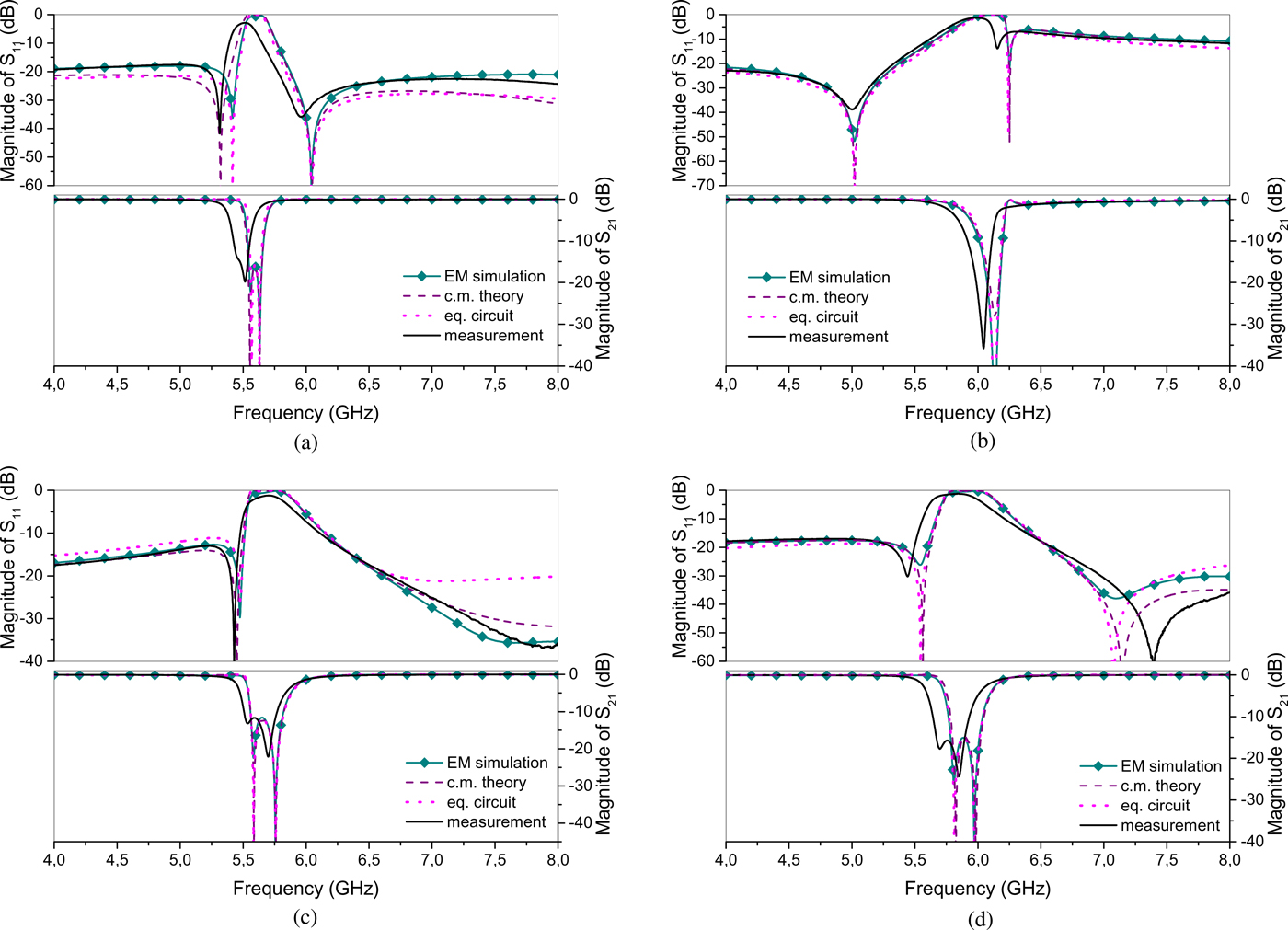
New results for all models in Fig. 2 are shown in Fig. 12, and parameters, obtained by the above procedure, are summarized in Table 4. This time, very good agreement has been obtained, not just for S ₂₁ but also for S ₁₁, in the whole bandwidth of one octave. Overall, CMT and equivalent circuit model produce equally good results, the only exception being slight mismatch in the first $S_{11}$ minimum on Fig. 12a. Considering the measurements in Fig. 12, it can be seen that the resonances are wider and shifted to lower frequencies. This is attributed to the presence of losses, which are left out from the EM simulations and analytical studies. It can also be noted that in some cases, such as in Fig. 12b, only a single resonance is visible in the transmission, because the frequency splitting is too small compared to the resonant widths.

Fig. 12. Comparison of magnitudes of S-parameters, obtained by simulation, measurement, equivalent circuit and coupled-mode theory, for the model in Fig. 2a (a), Fig. 2b (b), Fig. 2c (c), and Fig. 2d (d).

Table 4. Improved results obtained for the models in Fig. 2.

By examining the values in Table 4, we can observe that total coupling strength (which may be estimated as $\gamma _+ + \gamma _-$) increases as the SRR gap is moved away from the TL. This can be explained by the current distribution of the SRR, which has the biggest intensity in the arm opposite to the gap. It can also be seen that the fitted values of TL characteristic impedance used in CMT model (Fig. 7b), defined as $Z_C = \sqrt {L/C}$, also varies (last two rows of Table 4). This effect can be explained by the perturbation due to coupling, and it also explains disagreement in the preceding section, since there this perturbation is not accounted for. Consistently, variation in $Z_C$ is largest for the case of strongest coupling (Fig. 2b). Finally, it can also be seen that the coupling causes resonances to shift to higher frequencies.