


1 Introduction and overview
A canonical problem in free-surface hydrodynamics is that in which a fluid flowing at constant depth and speed in a horizontal channel encounters some sort of blockage. This might occur as a surface disturbance from a ship or a hovercraft, or be due to some object such as a submarine within the water, or an obstruction such as a reef on the bottom. The question of interest is to determine what kind of flow patterns are formed behind the blockage when the fluid has a free surface that can deform in response to the presence of the obstruction. In addition to the fundamental scientific interest that such flows represent, they are clearly also of great relevance to an extensive range of applications, such as ship hydrodynamics, submarine and hydrofoil design, flows produced by reefs, and so on. An authoritative review of many flows of these types has been presented by Wehausen and Laitone [Reference Wehausen and Laitone52]. The book by Kostyukov [Reference Kostyukov33] presents many of the classical solutions for waves produced by ships in various situations and shows how to calculate the wave resistance of hulls and propellers. Some more recent methods for the numerical solution of steady free-surface flow problems are discussed by Vanden-Broeck [Reference Vanden-Broeck48].
An enormous amount of research has been undertaken on free-surface flows caused by obstructions, in particular, when the vast amount of literature on ship hydrodynamics is taken into account. For this reason, we restrict our attention here only to surface waves that have been generated by irregularities at the bottom of a running stream. However, even within this greatly reduced subset of such possible flows, the variety of cases to consider is enormous. Such flows can occur either as steady-state or time-dependent entities. In general, they would exist in three-dimensional geometry, with a wedge-shaped pattern of waves formed behind the obstacle. Such flows are discussed in detail by Wehausen and Laitone [Reference Wehausen and Laitone52] and in the text by Stoker [Reference Stoker43] who also presents photographs of three-dimensional ship-wave patterns. These patterns also occur in atmospheric cloud formations [Reference Sharman and Wurtele41, Reference Wurtele, Sharman and Datta54]. Furthermore, in fluids consisting of more than one layer, obstacles can induce waves at the free surface in addition to internal waves at the interface(s) between fluid layers; this results in extra wave drag on the obstacle, and some seafarers have even ascribed the sluggish motion of their ships in layered oceans to the presence of magical beings within the ocean grasping hold of the hull of their ship [Reference Yiğit and Medvedev55]Footnote 1 . Surface waves in the full three-dimensional geometry can become particularly complicated in water of finite lateral extent [Reference Terziev, Tezdogan, Oguz, Gourlay, Demirel and Incecik45, Reference Tuck46].
Here, we restrict our attention to the consideration of bottom-mounted obstacles in two-dimensional geometry only. The flow therefore occurs in vertical planes and does not vary laterally. The obstacle can thus be considered as a cylinder of effectively infinite width. Further, we consider here only fluids that are “ideal”, in the sense that they are assumed to be inviscid and incompressible, and which therefore flow irrotationally.
The study of steady-state planar flows of ideal fluids over bottom-mounted obstacles is classical, and is discussed in detail by Lamb [Reference Lamb34, Article 245], in a linearized approximation in which the height of the obstacle above the bottom is supposed to be small. The problem can be solved in a reasonably straightforward manner using Fourier transforms, and the free-surface shape is given as an integral (an inverse Fourier transform). The behaviour of this integral is critically dependent upon a dimensionless Froude number
 $$ \begin{align} F = c / \sqrt{gH} , \end{align} $$
in which c is the undisturbed speed of the fluid stream past the obstacle, H is the undisturbed stream depth and g is the downward acceleration due to gravity. Since it is a ratio of two speeds, the Froude number F is closely analogous to the more familiar Mach number of gas dynamics [Reference Anderson1, p. 8]. Lamb’s linearized solution shows that there are two distinct parameter regions, in which the behaviour of the free surface is quite different. In the supercritical case
 $F> 1$
, the integral in the formula for the surface elevation is convergent, and it unambiguously shows that waves are formed neither upstream nor downstream of the obstacle; the surface on both sides is flat and it merely rises above the obstacle before resuming its undisturbed height downstream. However, in the subcritical case
$F> 1$
, the integral in the formula for the surface elevation is convergent, and it unambiguously shows that waves are formed neither upstream nor downstream of the obstacle; the surface on both sides is flat and it merely rises above the obstacle before resuming its undisturbed height downstream. However, in the subcritical case
 $F < 1$
, the integral expression for the surface shape is formally divergent, since a pole singularity appears in the denominator of the integrand. Nevertheless, Lamb [Reference Lamb34, Article 245] shows how to interpret this integral in such a way that it gives a finite result and also satisfies the radiation condition that, for
$F < 1$
, the integral expression for the surface shape is formally divergent, since a pole singularity appears in the denominator of the integrand. Nevertheless, Lamb [Reference Lamb34, Article 245] shows how to interpret this integral in such a way that it gives a finite result and also satisfies the radiation condition that, for
 $F < 1$
, waves cannot exist far upstream of the body in steady flow. In the process, Lamb obtains a free-surface shape that is flat far ahead of the obstacle, and then dips over the bottom bump before forming a downstream wave train that extends to infinity. Furthermore, Lamb, in Article 247, shows that the amplitude of the waves formed far downstream is proportional to the quantity
$F < 1$
, waves cannot exist far upstream of the body in steady flow. In the process, Lamb obtains a free-surface shape that is flat far ahead of the obstacle, and then dips over the bottom bump before forming a downstream wave train that extends to infinity. Furthermore, Lamb, in Article 247, shows that the amplitude of the waves formed far downstream is proportional to the quantity
 $\exp ( - 1 / F^2 )$
. This intriguing observation is the basis of the “low-speed paradox”, in which the downstream wave amplitude decreases faster than exponentially as
$\exp ( - 1 / F^2 )$
. This intriguing observation is the basis of the “low-speed paradox”, in which the downstream wave amplitude decreases faster than exponentially as
 $F \rightarrow 0$
. Lamb’s Fourier transform solution fails to yield a steady-state solution for the critical speed
$F \rightarrow 0$
. Lamb’s Fourier transform solution fails to yield a steady-state solution for the critical speed
 $F = 1$
.
$F = 1$
.
Lamb [Reference Lamb34, Article 247] illustrated his techniques to solve for the steady-state problem of free-surface flow over a semicircular cylinder of radius
 $\alpha $
placed across the bottom of a stream. The height
$\alpha $
placed across the bottom of a stream. The height
 $\alpha $
of the bump (and therefore also its total width
$\alpha $
of the bump (and therefore also its total width
 $2 \alpha $
) was assumed to be small, so that a linearized solution could be obtained. This problem of “ideal” fluid flow over a semicircle was reconsidered in the nonlinear context by Forbes and Schwartz [Reference Forbes and Schwartz19]. They used the Zhukovskii conformal transformation to map the bottom shape simply to a straight line, and thus enforced the bottom boundary condition on the semicircle exactly. They also calculated a linearized solution, valid for small semicircle radius
$2 \alpha $
) was assumed to be small, so that a linearized solution could be obtained. This problem of “ideal” fluid flow over a semicircle was reconsidered in the nonlinear context by Forbes and Schwartz [Reference Forbes and Schwartz19]. They used the Zhukovskii conformal transformation to map the bottom shape simply to a straight line, and thus enforced the bottom boundary condition on the semicircle exactly. They also calculated a linearized solution, valid for small semicircle radius
 $\alpha $
, and obtained essentially the same free-surface profile as Lamb [Reference Lamb34, Article 247], except that their downstream waves had exactly twice the amplitude of those calculated by Lamb. They attributed this difference to the fact that their linearized solution is no longer just a small perturbation about uniform flow, but instead represents a perturbation about a base flow that takes exact account of the semicircular bottom bump, including the two stagnation points on the bottom, as a result of the conformal mapping. They obtained numerical solutions to the nonlinear problem, based on a boundary-integral formulation, and computed solutions for
$\alpha $
, and obtained essentially the same free-surface profile as Lamb [Reference Lamb34, Article 247], except that their downstream waves had exactly twice the amplitude of those calculated by Lamb. They attributed this difference to the fact that their linearized solution is no longer just a small perturbation about uniform flow, but instead represents a perturbation about a base flow that takes exact account of the semicircular bottom bump, including the two stagnation points on the bottom, as a result of the conformal mapping. They obtained numerical solutions to the nonlinear problem, based on a boundary-integral formulation, and computed solutions for
 $F < 1$
having an evanescent surface shape upstream of the semicircle followed by a downstream nonlinear wave train. In the supercritical case
$F < 1$
having an evanescent surface shape upstream of the semicircle followed by a downstream nonlinear wave train. In the supercritical case
 $F> 1$
, they obtained wave-free surface profiles symmetric about the centre-plane
$F> 1$
, they obtained wave-free surface profiles symmetric about the centre-plane
 $x = 0$
. They were not able to compute wave-like solutions in the transcritical region near the critical value
$x = 0$
. They were not able to compute wave-like solutions in the transcritical region near the critical value
 $F = 1$
, but they speculated that nonlinear effects might allow such waves to exist for an appropriately large semicircle radius
$F = 1$
, but they speculated that nonlinear effects might allow such waves to exist for an appropriately large semicircle radius
 $\alpha $
. For both types of solution at each Froude number F, there was found to be a maximum bump size
$\alpha $
. For both types of solution at each Froude number F, there was found to be a maximum bump size
 $\alpha $
at which the free surface formed crests enclosing the Stokes angle of
$\alpha $
at which the free surface formed crests enclosing the Stokes angle of
 $120^{\circ }$
. Steady-state solutions for larger obstacles could not be found. Later, Vanden-Broeck [Reference Vanden-Broeck47] demonstrated that the supercritical wave-free solution is nonunique and that two such flows are possible. The first is the one computed by Forbes and Schwartz and is an analytical continuation of the linearized solution of Lamb, but a second solution also exists, and may be regarded as a bifurcation from a soliton.
$120^{\circ }$
. Steady-state solutions for larger obstacles could not be found. Later, Vanden-Broeck [Reference Vanden-Broeck47] demonstrated that the supercritical wave-free solution is nonunique and that two such flows are possible. The first is the one computed by Forbes and Schwartz and is an analytical continuation of the linearized solution of Lamb, but a second solution also exists, and may be regarded as a bifurcation from a soliton.
Zhang and Zhu [Reference Zhang and Zhu58] later reconsidered the results of Forbes and Schwartz for flow over a submerged semicircle, computing the steady nonlinear solutions using an integral equation based on hodograph variables. They obtained accurate numerical free-surface profiles and undertook a careful comparison with both the linearized solution and the results of Forbes and Schwartz. More recently, Pethiyagoda et al. [Reference Pethiyagoda, Moroney and McCue40] have argued that boundary-integral numerical methods require a very large number of numerical points on the free surface in order to maintain accuracy, and this requires a large nonlinear system of algebraic equations to be solved for the surface shape. It can be argued that the solution of this algebraic system must be carried out by a technique such as Newton’s method, which would solve a linear system exactly [Reference Forbes15] when
 $F < 1$
, and this then leads to the requirement that a large Jacobian matrix of derivatives be calculated and inverted at each iteration of the method. Pethiyagoda et al. [Reference Pethiyagoda, Moroney and McCue40] used an integral-equation approach closely related to that of Zhang and Zhu, but they devised an approach whereby they could avoid the explicit use of a Jacobian matrix. This allowed them to use many more free-surface points and to investigate numerical convergence of their scheme in considerable detail.
$F < 1$
, and this then leads to the requirement that a large Jacobian matrix of derivatives be calculated and inverted at each iteration of the method. Pethiyagoda et al. [Reference Pethiyagoda, Moroney and McCue40] used an integral-equation approach closely related to that of Zhang and Zhu, but they devised an approach whereby they could avoid the explicit use of a Jacobian matrix. This allowed them to use many more free-surface points and to investigate numerical convergence of their scheme in considerable detail.
In linearized theory of the type presented by Lamb [Reference Lamb34], two-dimensional steady flow over a bump suggests the possibility that, for obstacles of certain critical lengths, the free-surface waves generated at the front of the bump may be exactly half a wavelength out of phase with those produced at the back. Since, in linearized theory, these two wave trains superpose, the downstream waves cancel completely, leaving a subcritical flow that is nevertheless free of waves either side of the body. Forbes [Reference Forbes13] investigated this numerically for nonlinear flow over a semielliptical bump and found that there appeared to be ellipse lengths for which the downstream waves vanished. He followed this with a paper that sought wave-free subcritical solutions explicitly [Reference Forbes14], by demanding symmetric flow and making the numerical scheme compute the ellipse length for which this occurred. Remarkably, such drag-free solutions do occur, evidently for a countably infinite set of ellipse lengths agreeing very closely with the predictions of linearized theory for small ellipse heights; the nth such waveless flow contains
 $n - 1$
trapped waves over the ellipse, but none downstream. As the ellipse height is increased, however, these wave-free eigenfunctions begin to merge, and eventually coalesce in pairs at certain maximum ellipse heights. This intriguing result represents a relatively rare instance of an effective superposition principle present even in a nonlinear system, although the ellipse lengths for which it occurs depend strongly on the ellipse height, unlike the linearized system. As such, it is perhaps reminiscent of the celebrated result of Zabusky and Kruskal [Reference Zabusky and Kruskal56] for the Korteweg–de Vries equation. Later, Holmes et al. [Reference Holmes, Hocking, Forbes and Baillard29] and Hocking et al. [Reference Hocking, Holmes and Forbes27] carried out similar and more accurate computations for steady flow over a system of two bottom bumps, and confirmed the existence of sets of separation distances between the bumps for which wave-free solutions exist; furthermore, they allowed these bumps to have either positive or negative heights, and obtained an elaborate lattice of waveless solutions in a parameter space consisting of the separation distance and height of the two bumps. These results were extended by Holmes and Hocking [Reference Holmes and Hocking28], who also compared the fully nonlinear solutions with the predictions of weakly nonlinear theory.
$n - 1$
trapped waves over the ellipse, but none downstream. As the ellipse height is increased, however, these wave-free eigenfunctions begin to merge, and eventually coalesce in pairs at certain maximum ellipse heights. This intriguing result represents a relatively rare instance of an effective superposition principle present even in a nonlinear system, although the ellipse lengths for which it occurs depend strongly on the ellipse height, unlike the linearized system. As such, it is perhaps reminiscent of the celebrated result of Zabusky and Kruskal [Reference Zabusky and Kruskal56] for the Korteweg–de Vries equation. Later, Holmes et al. [Reference Holmes, Hocking, Forbes and Baillard29] and Hocking et al. [Reference Hocking, Holmes and Forbes27] carried out similar and more accurate computations for steady flow over a system of two bottom bumps, and confirmed the existence of sets of separation distances between the bumps for which wave-free solutions exist; furthermore, they allowed these bumps to have either positive or negative heights, and obtained an elaborate lattice of waveless solutions in a parameter space consisting of the separation distance and height of the two bumps. These results were extended by Holmes and Hocking [Reference Holmes and Hocking28], who also compared the fully nonlinear solutions with the predictions of weakly nonlinear theory.
In addition to the subcritical wave-like solutions (
 $F < 1$
) and the symmetric supercritical (
$F < 1$
) and the symmetric supercritical (
 $F> 1$
) wave-free solutions, there also exists a third solution type for steady-state flow. These are well known in the civil engineering literature, where they are often referred to as “critical flows” or “hydraulic falls”, and are discussed in the text by Henderson [Reference Henderson24]. In these flow types, there is subcritical flow ahead of the obstacle, and wave-free supercritical flow behind it. The fluid falls over the obstacle in a type of waterfall flow, and there is a point on it where the local Froude number equals one. Here, the obstacle is acting as a weir, choking the flow so that only a fixed steady volume flux is possible for a given obstacle height. Such steady solutions can only occur at one value of the upstream Froude number F for each value of the obstacle height
$F> 1$
) wave-free solutions, there also exists a third solution type for steady-state flow. These are well known in the civil engineering literature, where they are often referred to as “critical flows” or “hydraulic falls”, and are discussed in the text by Henderson [Reference Henderson24]. In these flow types, there is subcritical flow ahead of the obstacle, and wave-free supercritical flow behind it. The fluid falls over the obstacle in a type of waterfall flow, and there is a point on it where the local Froude number equals one. Here, the obstacle is acting as a weir, choking the flow so that only a fixed steady volume flux is possible for a given obstacle height. Such steady solutions can only occur at one value of the upstream Froude number F for each value of the obstacle height
 $\alpha $
. Forbes [Reference Forbes16] used the conformal map and boundary-integral approach of [Reference Forbes and Schwartz19] to compute steady critical flows produced by a semicircular bottom bump, allowing the upstream Froude number F in (1.1) to be found as an unknown parameter in the numerical scheme. He computed free-surface profiles and a portion of the subcritical F–
$\alpha $
. Forbes [Reference Forbes16] used the conformal map and boundary-integral approach of [Reference Forbes and Schwartz19] to compute steady critical flows produced by a semicircular bottom bump, allowing the upstream Froude number F in (1.1) to be found as an unknown parameter in the numerical scheme. He computed free-surface profiles and a portion of the subcritical F–
 $\alpha $
relationship for these flows, and also compared his results against experimentally measured values of the downstream fluid depth. A picture of one such flow is presented in Figure 1
Footnote
2
. Steady critical flows have since been computed for flows over various different bottom shapes, and some examples for flows over steps and rectangular obstacles are presented by Binder et al. [Reference Binder, Dias and Vanden-Broeck5].
$\alpha $
relationship for these flows, and also compared his results against experimentally measured values of the downstream fluid depth. A picture of one such flow is presented in Figure 1
Footnote
2
. Steady critical flows have since been computed for flows over various different bottom shapes, and some examples for flows over steps and rectangular obstacles are presented by Binder et al. [Reference Binder, Dias and Vanden-Broeck5].
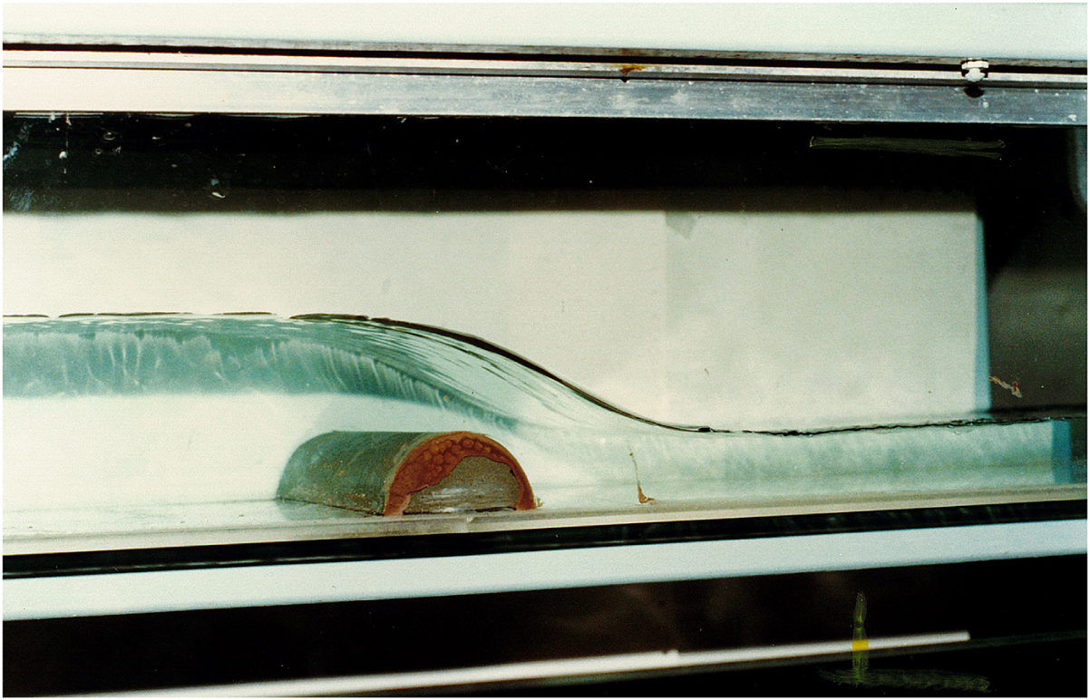
Figure 1 A photograph of a critical flow over a semicircular obstacle mounted on the bottom of a horizontal channel.
Because the calculation of nonlinear free-surface flows is difficult and computer-intensive, many researchers have been attracted to the use of simpler, weakly nonlinear theories to model such flows and, until the past two decades, these two approaches had proceeded almost independently and in parallel. Many of these more approximate analyses focused on the use of the Korteweg–de Vries (KdV) equation for two-dimensional flow, and Shen and Shen [Reference Shen and Shen42] present a concise picture of the predictions of KdV theory for steady free-surface flow over a bump. If the bottom disturbance is taken to be a semicircle, as assumed by both Forbes and Schwartz [Reference Forbes and Schwartz19] and Shen and Shen [Reference Shen and Shen42], then there are only two dimensionless parameters that describe the steady free-surface flow over this object. The first is the Froude number F in (1.1) and the second is the semicircle radius
 $\alpha $
. Suppose we fix the upstream speed
$\alpha $
. Suppose we fix the upstream speed
 $F < 1$
and consider the change of the behaviour of the (subcritical) solution as the bump radius
$F < 1$
and consider the change of the behaviour of the (subcritical) solution as the bump radius
 $\alpha $
is increased; according to KdV theory, the wavelength and the wave amplitude of the downstream waves increases until a finite value of
$\alpha $
is increased; according to KdV theory, the wavelength and the wave amplitude of the downstream waves increases until a finite value of
 $\alpha $
is reached at which the wavelength becomes infinite. Thus, in KdV theory, the downstream waves evolve continuously into the critical flow solution in Figure 1 as
$\alpha $
is reached at which the wavelength becomes infinite. Thus, in KdV theory, the downstream waves evolve continuously into the critical flow solution in Figure 1 as
 $\alpha $
increases, and there is no longer a steady solution once
$\alpha $
increases, and there is no longer a steady solution once
 $\alpha $
exceeds this limiting value. This is an elegant explanation for both the subcritical solution with downstream waves and the critical flow type, and it gives an appealing synthesis of the two. Unfortunately, this pleasing explanation is not confirmed by fully nonlinear calculations, which instead show that, as
$\alpha $
exceeds this limiting value. This is an elegant explanation for both the subcritical solution with downstream waves and the critical flow type, and it gives an appealing synthesis of the two. Unfortunately, this pleasing explanation is not confirmed by fully nonlinear calculations, which instead show that, as
 $\alpha $
is increased, the downstream waves shorten rather than lengthen, and although there is a limit radius
$\alpha $
is increased, the downstream waves shorten rather than lengthen, and although there is a limit radius
 $\alpha $
for these steady solutions, it is characterized by the breaking of the downstream waves at their crests, and is thus not related to the formation of the critical flow solution. Belward and Forbes [Reference Belward and Forbes3] computed both the solution type with downstream waves and the critical flow type for
$\alpha $
for these steady solutions, it is characterized by the breaking of the downstream waves at their crests, and is thus not related to the formation of the critical flow solution. Belward and Forbes [Reference Belward and Forbes3] computed both the solution type with downstream waves and the critical flow type for
 $F < 1$
and argued that there are parameter regions for which both steady solution types could exist simultaneously. However, Higgins et al. [Reference Higgins, Read and Belward26] later disputed this claim, arguing instead that the boundary-integral method of Belward and Forbes [Reference Belward and Forbes3] lacked sufficient accuracy to guarantee such a conclusion. The relationship, if any, between subcritical flows and critical flows therefore remains an open question.
$F < 1$
and argued that there are parameter regions for which both steady solution types could exist simultaneously. However, Higgins et al. [Reference Higgins, Read and Belward26] later disputed this claim, arguing instead that the boundary-integral method of Belward and Forbes [Reference Belward and Forbes3] lacked sufficient accuracy to guarantee such a conclusion. The relationship, if any, between subcritical flows and critical flows therefore remains an open question.
A recent review of the steady flow types predicted by KdV theory has been given by Binder [Reference Binder4]. That article examines various types of obstructions both mounted on the bottom and present at the free surface, and it carries out an extensive phase-plane analysis of the KdV model for these flows. Several authors have also investigated the use of other, similar, weakly nonlinear theories to describe flow over obstacles. Marchant and Smyth [Reference Marchant and Smyth38] derived a fifth-order KdV-type equation to describe unsteady flows over obstacles and compared their results with experiment. For unsteady flows, more elaborate approximations such as the Green–Naghdi equations [Reference Ertekin, Webster and Wehausen12] or Wu’s equations [Reference Lee, Yates and Wu35] have also been investigated, and the review by Helfrich and Melville [Reference Helfrich and Melville23] discusses further extensions of KdV-type models. Several more recent papers have also examined the accuracy of KdV theory against the predictions of fully nonlinear inviscid free-surface hydrodynamics. Holmes and Hocking [Reference Holmes and Hocking28] found that KdV theory was only accurate for flow over topography when
 $F \approx 1$
, which is entirely consistent with the approximation used in the derivation of that theory. Tam et al. [Reference Tam, Yu, Kelso and Binder44] used both KdV theory and fully nonlinear models to solve the (inverse) problem in which the free-surface elevation is assumed known, for a critical flow, and the bottom bump shape then calculated. They were able to obtain reasonable agreement with experiment only with fully nonlinear theory, and the KdV model was only able to predict coarse features of the underlying topology.
$F \approx 1$
, which is entirely consistent with the approximation used in the derivation of that theory. Tam et al. [Reference Tam, Yu, Kelso and Binder44] used both KdV theory and fully nonlinear models to solve the (inverse) problem in which the free-surface elevation is assumed known, for a critical flow, and the bottom bump shape then calculated. They were able to obtain reasonable agreement with experiment only with fully nonlinear theory, and the KdV model was only able to predict coarse features of the underlying topology.
As discussed previously, the linearized theory of Lamb [Reference Lamb34, Article 247] indicates that, for the subcritical flow
 $F < 1$
, the downstream wave amplitude is proportional to the quantity
$F < 1$
, the downstream wave amplitude is proportional to the quantity
 $\exp ( - 1 / F^2 )$
, which approaches zero faster than any power of
$\exp ( - 1 / F^2 )$
, which approaches zero faster than any power of
 $F^2$
as
$F^2$
as
 $F \rightarrow 0$
. Consequently, any attempt to create a “linearized” steady solution by expanding in powers of
$F \rightarrow 0$
. Consequently, any attempt to create a “linearized” steady solution by expanding in powers of
 $F^2$
(rather than the obstacle height, as in Lamb’s solution) will encounter difficulties, since the naïve series can be expected to be divergent and not to predict waves. In some free-surface fluid-flow problems, such as the canonical problem of flow generated by a submerged line or point source in otherwise stationary fluid, there is only the single dimensionless parameter
$F^2$
(rather than the obstacle height, as in Lamb’s solution) will encounter difficulties, since the naïve series can be expected to be divergent and not to predict waves. In some free-surface fluid-flow problems, such as the canonical problem of flow generated by a submerged line or point source in otherwise stationary fluid, there is only the single dimensionless parameter
 $F^2$
, so that linearization in the sense of Lamb’s solution is simply not possible. Consequently, expansions in powers of
$F^2$
, so that linearization in the sense of Lamb’s solution is simply not possible. Consequently, expansions in powers of
 $F^2$
give only asymptotic series, although it is nevertheless well known that such expressions can be remarkably accurate when only the first few terms in the series are retained; this was discussed for the problem of source flow by Peregrine [Reference Peregrine39] in two dimensions and by Forbes and Hocking [Reference Forbes and Hocking18] in three-dimensional geometry. Possibly the first serious attempt to obtain detailed information from a high-order (divergent) series expansion in powers of
$F^2$
give only asymptotic series, although it is nevertheless well known that such expressions can be remarkably accurate when only the first few terms in the series are retained; this was discussed for the problem of source flow by Peregrine [Reference Peregrine39] in two dimensions and by Forbes and Hocking [Reference Forbes and Hocking18] in three-dimensional geometry. Possibly the first serious attempt to obtain detailed information from a high-order (divergent) series expansion in powers of
 $F^2$
was made by Vanden-Broeck et al. [Reference Vanden-Broeck, Schwartz and Tuck49]. They used computer arithmetic to generate the coefficients of the series expansions in
$F^2$
was made by Vanden-Broeck et al. [Reference Vanden-Broeck, Schwartz and Tuck49]. They used computer arithmetic to generate the coefficients of the series expansions in
 $F^2$
, and they observed that such series are indeed divergent with the nth order coefficient behaving like
$F^2$
, and they observed that such series are indeed divergent with the nth order coefficient behaving like
 $n!$
. By using numerical series-acceleration techniques (the Shanks transformation), they were able to “sum” their divergent series, and for flow past a surface-piercing ship in planar geometry, their result indicated a free surface, behind the ship, that was wave-free but possessed a discontinuity. Vanden-Broeck et al. [Reference Vanden-Broeck, Schwartz and Tuck49] interpreted this to mean that there were two different solutions, and their series-summation technique was giving the wave-free portions of each; the discontinuity at the free surface represented their technique attempting to connect their two solution portions with a branch cut. In fact, by interpreting the portion between the ship and the discontinuity as representing a section of a genuine stern flow, they used an integral-equation formulation to “complete” the downstream flow, and they did indeed obtain a steady-state stern flow with a train of downstream waves.
$n!$
. By using numerical series-acceleration techniques (the Shanks transformation), they were able to “sum” their divergent series, and for flow past a surface-piercing ship in planar geometry, their result indicated a free surface, behind the ship, that was wave-free but possessed a discontinuity. Vanden-Broeck et al. [Reference Vanden-Broeck, Schwartz and Tuck49] interpreted this to mean that there were two different solutions, and their series-summation technique was giving the wave-free portions of each; the discontinuity at the free surface represented their technique attempting to connect their two solution portions with a branch cut. In fact, by interpreting the portion between the ship and the discontinuity as representing a section of a genuine stern flow, they used an integral-equation formulation to “complete” the downstream flow, and they did indeed obtain a steady-state stern flow with a train of downstream waves.
The more recent development of techniques for analysing these divergent series in the Froude number has enabled the phenomenon of the downstream waves behind bottom topography to be understood from a different perspective. Chapman and Vanden-Broeck [Reference Chapman and Vanden-Broeck7] employed the theory of exponential asymptotics to study steady-state flow over a step on the bottom of a channel, and thus re-examined an earlier paper by King and Bloor [Reference King and Bloor31] who had solved this problem using an integral-equation approach. Chapman and Vanden-Broeck found that their technique generated a Stokes line, at which waves of exponentially small amplitude could be produced. This line started from one corner of the bottom-based step and moved through the fluid until it intersected the free surface; this is reminiscent of the discontinuous jump at the free surface that the Shanks-transform series-summation method of Vanden-Broeck et al. [Reference Vanden-Broeck, Schwartz and Tuck49] had similarly produced. This work was later generalized by Lustri et al. [Reference Lustri, McCue and Binder37] to allow the bottom-based step to have a finite slope.
The solutions for flow over topography discussed so far have all been for the steady-state case, but it is not always obvious whether such solutions would be observable once transient (time-dependent) behaviour is also considered. In the laboratory, two-dimensional flows of the type studied in this paper would be achieved by placing a cylindrical obstruction across the bottom of a rectangular channel and avoiding boundary-layer effects at the channel walls. The steady-state flow presumably then corresponds to infinite-time behaviour
 $t \rightarrow \infty $
, and so questions of stability naturally arise. For supercritical flow upstream,
$t \rightarrow \infty $
, and so questions of stability naturally arise. For supercritical flow upstream,
 $F> 1$
, it seems likely that one of Vanden-Broeck’s two steady solutions would be unstable [Reference Vanden-Broeck47] and thus would not be seen. By contrast, the “critical” flow type, in which there is an hydraulic fall over the obstacle, is easily generated, is stable, as Figure 1 indicates, and agrees well with nonlinear numerical solutions of the steady equations [Reference Forbes16].
$F> 1$
, it seems likely that one of Vanden-Broeck’s two steady solutions would be unstable [Reference Vanden-Broeck47] and thus would not be seen. By contrast, the “critical” flow type, in which there is an hydraulic fall over the obstacle, is easily generated, is stable, as Figure 1 indicates, and agrees well with nonlinear numerical solutions of the steady equations [Reference Forbes16].
The situation for time-dependent subcritical flow
 $F < 1$
is much less clear. For a bottom bump placed across a channel with parallel vertical walls, Ertekin et al. [Reference Ertekin, Webster and Wehausen11] demonstrated experimentally that a train of solitons is generated ahead of the obstruction and, as time progresses, these waves move further upstream. This observation was supported by numerical solutions of approximate, weakly nonlinear models in a later paper by the same authors [Reference Ertekin, Webster and Wehausen12]. These upstream-advancing solitons have since generated a great deal of interest. Wu [Reference Wu53] used a weakly nonlinear theory (Wu’s equations) to compute unsteady flow over topography at the critical Froude number
$F < 1$
is much less clear. For a bottom bump placed across a channel with parallel vertical walls, Ertekin et al. [Reference Ertekin, Webster and Wehausen11] demonstrated experimentally that a train of solitons is generated ahead of the obstruction and, as time progresses, these waves move further upstream. This observation was supported by numerical solutions of approximate, weakly nonlinear models in a later paper by the same authors [Reference Ertekin, Webster and Wehausen12]. These upstream-advancing solitons have since generated a great deal of interest. Wu [Reference Wu53] used a weakly nonlinear theory (Wu’s equations) to compute unsteady flow over topography at the critical Froude number
 $F = 1$
and demonstrated the presence of the upstream train of solitons and a downstream pattern of waves moving away from the disturbance. Similar computations were also carried out by Lee et al. [Reference Lee, Yates and Wu35], again using Wu’s equations, and they also demonstrated that their results were in accordance with experimental measurements for Froude numbers in the transcritical range
$F = 1$
and demonstrated the presence of the upstream train of solitons and a downstream pattern of waves moving away from the disturbance. Similar computations were also carried out by Lee et al. [Reference Lee, Yates and Wu35], again using Wu’s equations, and they also demonstrated that their results were in accordance with experimental measurements for Froude numbers in the transcritical range
 $F \approx 1$
. Recall that Lamb’s linearized solution [Reference Lamb34, Article 247] for steady flow fails at the critical value
$F \approx 1$
. Recall that Lamb’s linearized solution [Reference Lamb34, Article 247] for steady flow fails at the critical value
 $F = 1$
, and it has been demonstrated by Cole [Reference Cole10] that the corresponding linearized theory for unsteady flow predicts that the free-surface elevation grows like
$F = 1$
, and it has been demonstrated by Cole [Reference Cole10] that the corresponding linearized theory for unsteady flow predicts that the free-surface elevation grows like
 $t^{1/3}$
for large t, for critical flow
$t^{1/3}$
for large t, for critical flow
 $F = 1$
. Some degree of nonlinearity is therefore required to obtain solutions in the transcritical regime, and Cole used KdV theory to obtain these; her results are qualitatively equivalent to those of Wu [Reference Wu53] obtained with a different weakly nonlinear model. The use of KdV theory to calculate unsteady flow over a step is reviewed by Grimshaw [Reference Grimshaw21], and KdV theory has also been used in a variety of other applications, including waves generated by two bottom bumps [Reference Chardard, Dias, Nguyen and Vanden-Broeck8, Reference Grimshaw and Maleewong22].
$F = 1$
. Some degree of nonlinearity is therefore required to obtain solutions in the transcritical regime, and Cole used KdV theory to obtain these; her results are qualitatively equivalent to those of Wu [Reference Wu53] obtained with a different weakly nonlinear model. The use of KdV theory to calculate unsteady flow over a step is reviewed by Grimshaw [Reference Grimshaw21], and KdV theory has also been used in a variety of other applications, including waves generated by two bottom bumps [Reference Chardard, Dias, Nguyen and Vanden-Broeck8, Reference Grimshaw and Maleewong22].
In this article, we consider the time-dependent linearized solution, based on Lamb’s [Reference Lamb34] formulation. We also present some solutions to the full nonlinear system of inviscid free-surface equations, using a novel spectral method based on one developed by Forbes et al. [Reference Forbes, Chen and Trenham17] for free-surface flows, but extended here to permit arbitrary smooth bottom-bump topography.
2 Unsteady spectral formulation
We now consider a novel semianalytical approach to the description of the unsteady two-dimensional problem of flow over an obstacle. A Cartesian coordinate system is located with its x-axis pointing horizontally along the bottom and its y-axis pointing vertically, as in Figure 2. The fluid is subject to the gravitational body force, with constant acceleration g directed negatively along the y-axis. As in earlier works [Reference Forbes and Schwartz19, Reference Lamb34], the fluid is taken to be inviscid and incompressible, so that its velocity vector
 $\mathbf {q} ( x,y,t ) \equiv u ( x,y,t ) \mathbf {i} + v ( x,y,t ) \mathbf {j}$
can be written as the gradient of a velocity potential
$\mathbf {q} ( x,y,t ) \equiv u ( x,y,t ) \mathbf {i} + v ( x,y,t ) \mathbf {j}$
can be written as the gradient of a velocity potential
 $\Phi ( x,y,t )$
in the form
$\Phi ( x,y,t )$
in the form
 $\mathbf {q} = \nabla \Phi $
. Here, the two constant unit vectors
$\mathbf {q} = \nabla \Phi $
. Here, the two constant unit vectors
 $\mathbf {i}$
and
$\mathbf {i}$
and
 $\mathbf {j}$
point along the positive x- and y-axes, respectively. The governing equation in the fluid is then Laplace’s equation
$\mathbf {j}$
point along the positive x- and y-axes, respectively. The governing equation in the fluid is then Laplace’s equation
 $$ \begin{align} \nabla^2 \Phi = \partial^2 \Phi / \partial x^2 + \partial^2 \Phi / \partial y^2 = 0. \end{align} $$
In the absence of any obstacle, the fluid would simply be flowing from left to right with some uniform speed c and have constant depth H.


We now introduce dimensionless variables, which we will use henceforth. All lengths are referenced to the undisturbed fluid depth H, and speeds are referred to c. The scale for time is chosen to be
 $H/c$
. In these nondimensional coordinates, the upstream speed and depth of the fluid are both one, as depicted in Figure 2. The form of the governing equation (2.1) remains unchanged by this transformation. The key dimensionless parameter is seen to be the Froude number F in (1.1), although there will be two further dimensionless constants
$H/c$
. In these nondimensional coordinates, the upstream speed and depth of the fluid are both one, as depicted in Figure 2. The form of the governing equation (2.1) remains unchanged by this transformation. The key dimensionless parameter is seen to be the Froude number F in (1.1), although there will be two further dimensionless constants
 $\alpha $
and
$\alpha $
and
 $\beta $
which will specify the length and the height of the bottom-based obstruction, respectively. Clearly, the height
$\beta $
which will specify the length and the height of the bottom-based obstruction, respectively. Clearly, the height
 $\beta $
provides a direct measure of the effects of nonlinearity, since, as
$\beta $
provides a direct measure of the effects of nonlinearity, since, as
 $\beta \rightarrow 0$
, the obstruction vanishes and simple uniform flow
$\beta \rightarrow 0$
, the obstruction vanishes and simple uniform flow
 $\Phi = x$
is restored.
$\Phi = x$
is restored.
For simplicity, we assume that the shape of the bottom-mounted obstacle does not change with time, and so we suppose it to be described by the equation
 $y = h (x)$
. For inviscid fluid, there can be no flow normal to the bottom, which gives the kinematic condition
$y = h (x)$
. For inviscid fluid, there can be no flow normal to the bottom, which gives the kinematic condition
 $$ \begin{align} v = u \frac {d h(x)}{d x} \quad \text{on } y = h(x) \end{align} $$
holding on the bottom surface.
A similar kinematic condition holds on the unknown location
 $y = \eta (x,t)$
of the free surface. Since this is a material boundary, taking the time derivative following the motion gives
$y = \eta (x,t)$
of the free surface. Since this is a material boundary, taking the time derivative following the motion gives
 $$ \begin{align} \frac {\partial \eta}{\partial t} = v - u \frac {\partial \eta}{\partial x} \quad \text{on } y = \eta (x,t). \end{align} $$
There is also a dynamic boundary condition that holds on the free surface, which expresses the fact that the pressure in the fluid there must be continuous with the (constant) atmospheric pressure. The fluid pressure can be calculated using Bernoulli’s equation, and, in dimensionless coordinates, the final form of this dynamic condition is
 $$ \begin{align} F^2 \frac {\partial \Phi}{\partial t} + \frac {1}{2} F^2 ( u^2 + v^2 ) + \eta = \frac {1}{2} F^2 + 1 \quad \text{on } y = \eta ( x,t ). \end{align} $$
The constant F is the Froude number in equation (1.1).
Forbes and Schwartz [Reference Forbes and Schwartz19] developed a numerical scheme for solving the steady version of this nonlinear inviscid problem (2.1)–(2.4). Their technique was based on the use of boundary-integral methods to satisfy (2.1) in the fluid region, replacing it with a singular integral equation that only involved variables on the free surface. Such an approach has obvious advantages, but, in the unsteady problem, it can lead to ill-conditioning, since the integral equation to be solved at each new time step is a Fredholm equation of the first kind. Here, we instead seek the numerical solution to the unsteady problem, in some computational window
 $-L < x < L$
, in the semianalytical form
$-L < x < L$
, in the semianalytical form
 $$ \begin{align} \Phi ( x,y,t ) & = x + \sum_{n=1}^N \bigg[ A_n (t) \cos \bigg( \frac {n \pi x}{L} \bigg) + B_n (t) \sin \bigg( \frac {n \pi x}{L} \bigg) \bigg] \frac {\cosh ( n \pi y / L )}{\cosh ( n \pi / L )} \nonumber \\ & \quad + \sum_{m=1}^M Q_m (t) \int_{-\alpha}^{\alpha} \sin \bigg( \frac {m \pi ( \xi + \alpha )}{2\alpha} \bigg) \ln \sqrt{ (x - \xi )^2 + y^2} \, d \xi. \end{align} $$
Here, the bump
 $y = h(x)$
on the bottom of the channel is supposed to have finite support, and to lie over the portion
$y = h(x)$
on the bottom of the channel is supposed to have finite support, and to lie over the portion
 $-\alpha < x < \alpha $
. Outside the interval, the bottom is simply the flat surface
$-\alpha < x < \alpha $
. Outside the interval, the bottom is simply the flat surface
 $y = 0$
. The aim is to find the Fourier coefficients
$y = 0$
. The aim is to find the Fourier coefficients
 $ A_n (t)$
,
$ A_n (t)$
,
 $B_n (t)$
and the coefficients
$B_n (t)$
and the coefficients
 $Q_m (t)$
of an effective distribution of sources along
$Q_m (t)$
of an effective distribution of sources along
 $-\alpha < x < \alpha $
,
$-\alpha < x < \alpha $
,
 $y = 0$
designed to enforce the bottom boundary condition (2.2). The velocity components u and v are then obtained by direct differentiation of the velocity potential (2.5).
$y = 0$
designed to enforce the bottom boundary condition (2.2). The velocity components u and v are then obtained by direct differentiation of the velocity potential (2.5).
The paper by Forbes and Schwartz [Reference Forbes and Schwartz19] used conformal mapping to enforce the bottom condition (2.2) exactly, and this is the most precise and accurate technique available. It also has the advantage that it copes exactly with corners in the bottom profile, where there might be a stagnation point or even a flow singularity in the inviscid flow model. The drawback of conformal mapping is that each specific bottom shape requires its own unique mapping function. Thus Forbes and Schwartz studied flow generated by a semicircular bump only, although Forbes [Reference Forbes14] generalized the mapping function to allow semielliptical obstacles, demonstrating, in the process, that exact wave cancellation could occur downstream for obstacles of the appropriate length and height, even in the nonlinear problem. These findings were confirmed later by Hocking et al. [Reference Hocking, Holmes and Forbes27] and Holmes et al. [Reference Holmes, Hocking, Forbes and Baillard29]. King and Bloor [Reference King and Bloor31] investigated free-surface flow produced by polygonal obstacles, and even devised a numerical conformal-mapping technique based on a continuous Schwarz–Christoffel mapping [Reference King and Bloor32]. More recent flows over rectangular obstacles have been presented by Herterich and Dias [Reference Herterich and Dias25].
In this present analysis based on (2.5), we have taken an alternative approach that allows for a general bottom profile
 $y = h(x)$
over some interval
$y = h(x)$
over some interval
 $-\alpha < x < \alpha $
, and thus we are not restricted only to profiles for which complex conformal mappings are known. However, our profiles are now required to be continuous and have continuous first derivatives, so that bottom corners and stagnation points are excluded here. For a bump having compact support, this necessarily means that
$-\alpha < x < \alpha $
, and thus we are not restricted only to profiles for which complex conformal mappings are known. However, our profiles are now required to be continuous and have continuous first derivatives, so that bottom corners and stagnation points are excluded here. For a bump having compact support, this necessarily means that
 $$ \begin{align} h (\pm\alpha ) = 0 \quad \text{and} \quad h' (\pm\alpha ) = 0. \end{align} $$
This, however, imposes no major limitation, since corners can always be approximated to some degree by a smooth curve, and, in fact, Fridman [Reference Fridman20] has argued that some two-dimensional flows replace a single stagnation point with a stagnation zone of finite area but shape that is unknown a priori; such inviscid flows possibly mimic closely the recirculating zone near a stagnation point expected in viscous fluids. In this representation (2.5), the second integral term can be regarded as a continuous line source distribution along the surface
 $y = 0$
, with effective source strength
$y = 0$
, with effective source strength
 $P_S(x,t)$
represented in the Fourier-series form
$P_S(x,t)$
represented in the Fourier-series form
 $$ \begin{align} P_S(x,t) = \sum_{m=1}^M Q_m (t) \sin \bigg( \frac {m \pi ( x + \alpha )}{2\alpha} \bigg). \end{align} $$
We observe that
 $P_S(x,t)$
falls to zero at
$P_S(x,t)$
falls to zero at
 $x = \pm \alpha $
due to the smoothness conditions (2.6).
$x = \pm \alpha $
due to the smoothness conditions (2.6).
In view of (2.5), the bottom condition (2.2) becomes
 $$ \begin{align} \sum_{m=1}^M Q_m (t) G^B_1 (x) = - h'(x) + \sum_{n=1}^N A_n (t) G^S_2 (x) + \sum_{n=1}^N B_n (t) G^S_3 (x) , \end{align} $$
where we have chosen to denote
 $$ \begin{align} \begin{aligned} G^B_1 (x) & = \int_{-\alpha}^{\alpha} \sin \bigg( \frac {m \pi ( \xi + \alpha )}{2\alpha} \bigg) \bigg[ \frac {(x - \xi )h'(x) - h(x)}{(x - \xi )^2 + h^2 (x)} \bigg] \, d \xi \\ G^S_2 (x) & = \frac {n\pi}{L} \bigg[ h'(x) \sin \bigg( \frac {n\pi x}{L} \bigg) \frac {\cosh ( n\pi h(x) / L )}{\cosh ( n\pi / L )} \\ & \quad + \cos \bigg( \frac {n\pi x}{L} \bigg) \frac {\sinh ( n\pi h(x) / L )}{\cosh ( n\pi / L )} \bigg] \\ G^S_3 (x) & = \frac {n\pi}{L} \bigg[ - h'(x) \cos \bigg( \frac {n\pi x}{L} \bigg) \frac {\cosh ( n\pi h(x) / L )}{\cosh ( n\pi / L )} \\ & \quad + \sin \bigg( \frac {n\pi x}{L} \bigg) \frac {\sinh ( n\pi h(x) / L )}{\cosh ( n\pi / L )} \bigg]. \end{aligned} \end{align} $$
This representation (2.8) of the bottom boundary condition (2.2) is now Fourier analysed by multiplying it by the basis functions
 $\sin ( k\pi (x + \alpha ) / (2\alpha ) )$
,
$\sin ( k\pi (x + \alpha ) / (2\alpha ) )$
,
 $k = 1 , 2 , \ldots , M$
, and integrating over the compact domain. The result is the
$k = 1 , 2 , \ldots , M$
, and integrating over the compact domain. The result is the
 $M \times M$
matrix system of linear equations
$M \times M$
matrix system of linear equations
 $$ \begin{align} \mathbf{L^B Q} = \mathbf{R^A A} + \mathbf{R^B B} - \mathbf{E^B} , \end{align} $$
in which the
 $M \times 1$
vector
$M \times 1$
vector
 $\mathbf {Q}$
contains the coefficients
$\mathbf {Q}$
contains the coefficients
 $Q_m (t)$
and the two
$Q_m (t)$
and the two
 $N \times 1$
vectors
$N \times 1$
vectors
 $\mathbf {A}$
and
$\mathbf {A}$
and
 $\mathbf {B}$
consist of elements
$\mathbf {B}$
consist of elements
 $A_n (t)$
and
$A_n (t)$
and
 $B_n (t)$
, respectively. The vector
$B_n (t)$
, respectively. The vector
 $\mathbf {E^B}$
has the M components
$\mathbf {E^B}$
has the M components
 $$ \begin{align*} E^B_k = \int_{-\alpha}^{\alpha} h'(x) \sin \bigg( \frac {k \pi ( x + \alpha )}{2\alpha} \bigg) \, d x \nonumber \end{align*} $$
and the two
 $M \times N$
matrices
$M \times N$
matrices
 $\mathbf {R^A}$
and
$\mathbf {R^A}$
and
 $\mathbf {R^B}$
contain elements
$\mathbf {R^B}$
contain elements
 $$ \begin{align*} R^A_{k,n} & = \int_{-\alpha}^{\alpha} G^S_2 (x) \sin \bigg( \frac {k \pi ( x + \alpha )}{2\alpha} \bigg) \, dx \nonumber \\ R^B_{k,n} & = \int_{-\alpha}^{\alpha} G^S_3 (x) \sin \bigg( \frac {k \pi ( x + \alpha )}{2\alpha} \bigg) \, dx .\nonumber \end{align*} $$
The
 $M \times M$
matrix
$M \times M$
matrix
 $\mathbf {L^B}$
has components
$\mathbf {L^B}$
has components
 $$ \begin{align*} L^B_{k,m} = \int_{-\alpha}^{\alpha} G^B_1 (x) \sin \bigg( \frac {k \pi ( x + \alpha )}{2\alpha} \bigg) \, d x. \nonumber \end{align*} $$
This matrix equation (2.10) is finally solved for the vector
 $\mathbf {Q}$
of bottom-profile coefficients
$\mathbf {Q}$
of bottom-profile coefficients
 $Q_m (t)$
, in terms of the free-surface coefficients
$Q_m (t)$
, in terms of the free-surface coefficients
 $A_n (t)$
and
$A_n (t)$
and
 $B_n (t)$
, and gives a matrix expression of the form
$B_n (t)$
, and gives a matrix expression of the form
 $$ \begin{align} \mathbf{Q} = \mathbf{T^A A} + \mathbf{T^B B} - \mathbf{F^B} , \end{align} $$
with
 $M \times N$
coefficient matrices
$M \times N$
coefficient matrices
 $$ \begin{align} \mathbf{T^A} = ( \mathbf{L^B} )^{-1} \mathbf{R^A} \quad \text{and} \quad \mathbf{T^B} = ( \mathbf{L^B} )^{-1} \mathbf{R^B} \end{align} $$
and
 $M \times 1$
vector
$M \times 1$
vector
 $$ \begin{align} \mathbf{F^B} = ( \mathbf{L^B} )^{-1} \mathbf{E^B}. \end{align} $$
In the numerical method, it is only necessary to calculate these matrices (2.12) and vector (2.13) once, since they are independent of time. Once obtained, they are stored and used later as needed.
The kinematic free-surface condition (2.3) is also subjected to Fourier decomposition, following the “basic” algorithm in the paper of Forbes et al. [Reference Forbes, Chen and Trenham17]. To begin, we define surface velocity components
 $$ \begin{align} U (x,t) = u ( x, \eta (x,t) , t ) \quad \text{and} \quad V (x,t) = v ( x, \eta (x,t) , t ) \end{align} $$
by direct differentiation of the velocity potential (2.5) and then evaluating the resulting expressions on the free surface
 $y = \eta (x,t)$
. A spectral representation is also needed for the unknown free-surface shape, which is consistent with (2.5), and we choose
$y = \eta (x,t)$
. A spectral representation is also needed for the unknown free-surface shape, which is consistent with (2.5), and we choose
 $$ \begin{align} \eta (x,t) = H_0 (t) + \sum_{n=1}^N \bigg[ H_n (t) \cos \bigg( \frac {n \pi x}{L} \bigg) + K_n (t) \sin \bigg( \frac {n \pi x}{L} \bigg) \bigg]. \end{align} $$
Next, the kinematic condition (2.3) at the free surface is multiplied by the appropriate basis functions and integrated over the computational domain
 $-L < x < L$
to give
$-L < x < L$
to give
 $$ \begin{align} \begin{aligned} H'_0 (t) & = \frac {1}{2L} \int_{-L}^L \bigg( V - U \frac {\partial \eta}{\partial x} \bigg) \, d x \\ H'_{\ell} (t) & = \frac {1}{L} \int_{-L}^L \bigg( V - U \frac {\partial \eta}{\partial x} \bigg) \cos \bigg( \frac {\ell\pi x}{L} \bigg) \, d x \\ K'_{\ell} (t) & = \frac {1}{L} \int_{-L}^L \bigg( V - U \frac {\partial \eta}{\partial x} \bigg) \sin \bigg( \frac {\ell\pi x}{L} \bigg) \, d x \\ & \quad \quad \quad \quad \ell = 1 , 2 , \ldots , N. \end{aligned} \end{align} $$
These represent a system of differential equations for the coefficients of the free-surface elevation in (2.15).
Finally, the dynamic free-surface condition (2.4) is subject to similar Fourier analysis at the surface. The two representations (2.5) and (2.15) for the velocity potential and surface shape are used, and the even Fourier modes are then obtained by multiplying by the even basis functions
 $\cos ( \ell \pi x / L )$
, for
$\cos ( \ell \pi x / L )$
, for
 $\ell = 1 , 2 , \ldots , N$
, and integrating over the computational window
$\ell = 1 , 2 , \ldots , N$
, and integrating over the computational window
 $- L < x < L$
. This gives an
$- L < x < L$
. This gives an
 $N \times N$
matrix equation of the form
$N \times N$
matrix equation of the form
 $$ \begin{align} F^2 \mathbf{C^C} \mathbf{A}' + F^2 \mathbf{C^S} \mathbf{B}' + F^2 \mathbf{\mathcal{M}} \mathbf{Q}' = -\mathbf{H} - \tfrac {1}{2} F^2 \mathbf{Y^C} , \end{align} $$
in which
 $\mathbf {A}$
, and so on, are the vectors of coefficients as previously, and the additional
$\mathbf {A}$
, and so on, are the vectors of coefficients as previously, and the additional
 $N \times 1$
vector
$N \times 1$
vector
 $\mathbf {H}$
contains the N coefficients
$\mathbf {H}$
contains the N coefficients
 $H_n (t)$
in (2.15). The two
$H_n (t)$
in (2.15). The two
 $N \times N$
matrices
$N \times N$
matrices
 $\mathbf {C^C}$
and
$\mathbf {C^C}$
and
 $\mathbf {C^S}$
have elements
$\mathbf {C^S}$
have elements
 $$ \begin{align} \begin{aligned} C^C_{\ell ,n} (t) & = \frac {1}{L} \int_{-L}^{L} \cos \bigg( \frac {n\pi x}{L} \bigg) \frac {\cosh ( n\pi \eta (x,t) / L )}{\cosh ( n\pi / L )} \cos \bigg( \frac {\ell \pi x}{L} \bigg) \, d x \\ C^S_{\ell ,n} (t) & = \frac {1}{L} \int_{-L}^{L} \sin \bigg( \frac {n\pi x}{L} \bigg) \frac {\cosh ( n\pi \eta (x,t) / L )}{\cosh ( n\pi / L )} \cos \bigg( \frac {\ell \pi x}{L} \bigg) \, d x \end{aligned} \end{align} $$
and the
 $N \times 1$
vector
$N \times 1$
vector
 $\mathbf {Y^C}$
has components
$\mathbf {Y^C}$
has components
 $$ \begin{align} Y^C_{\ell} (t) = \frac {1}{L} \int_{-L}^{L} ( U^2 + V^2 ) \cos \bigg( \frac {\ell \pi x}{L} \bigg) \, d x. \end{align} $$
Here, U and V are the two surface velocity components defined in (2.14). The
 $M \times N$
matrix
$M \times N$
matrix
 $\mathbf {\mathcal {M}}$
in (2.17) contains the elements
$\mathbf {\mathcal {M}}$
in (2.17) contains the elements
 $$ \begin{align} \mathcal{M}_{\ell ,m} (t) & = \frac {1}{L} \int_{-L}^{L} \cos \bigg( \frac {\ell \pi x}{L} \bigg) \, d x \nonumber \\ & \quad \times \int_{-\alpha}^{\alpha} \sin \bigg( \frac {m \pi ( \xi + \alpha )}{2\alpha} \bigg) \ln \sqrt{ (x - \xi )^2 + \eta^2 (x,t)} \, d \xi. \end{align} $$
The odd Fourier modes for the dynamic free-surface condition are likewise obtained by multiplying by the odd basis functions
 $\sin ( \ell \pi x / L )$
, for
$\sin ( \ell \pi x / L )$
, for
 $\ell = 1 , 2 , \ldots , N$
, and integrating. This gives the
$\ell = 1 , 2 , \ldots , N$
, and integrating. This gives the
 $N \times N$
matrix equation
$N \times N$
matrix equation
 $$ \begin{align} F^2 \mathbf{S^C} \mathbf{A}' + F^2 \mathbf{S^S} \mathbf{B}' + F^2 \mathbf{\mathcal{N}} \mathbf{Q}' = -\mathbf{K} - \tfrac {1}{2} F^2 \mathbf{Y^S}. \end{align} $$
Here, the
 $N \times 1$
vector
$N \times 1$
vector
 $\mathbf {K}$
contains the coefficients
$\mathbf {K}$
contains the coefficients
 $K_n (t)$
in (2.15). The two matrices
$K_n (t)$
in (2.15). The two matrices
 $\mathbf {S^C}$
and
$\mathbf {S^C}$
and
 $\mathbf {S^S}$
have the same form as
$\mathbf {S^S}$
have the same form as
 $\mathbf {C^C}$
and
$\mathbf {C^C}$
and
 $\mathbf {C^S}$
in the definitions (2.18), except that the quantity
$\mathbf {C^S}$
in the definitions (2.18), except that the quantity
 $\cos ( \ell \pi x / L )$
in the integrands must be replaced with
$\cos ( \ell \pi x / L )$
in the integrands must be replaced with
 $\sin ( \ell \pi x / L )$
. The vector
$\sin ( \ell \pi x / L )$
. The vector
 $\mathbf {Y^S}$
is obtained from the definition (2.19) by similarly substituting
$\mathbf {Y^S}$
is obtained from the definition (2.19) by similarly substituting
 $\sin ( \ell \pi x / L )$
in place of the cosine term, and the same substitution is used to obtain the elements of the
$\sin ( \ell \pi x / L )$
in place of the cosine term, and the same substitution is used to obtain the elements of the
 $M \times N$
matrix
$M \times N$
matrix
 $\mathbf {\mathcal {N}}$
in place of
$\mathbf {\mathcal {N}}$
in place of
 $\mathbf {\mathcal {M}}$
in equation (2.20).
$\mathbf {\mathcal {M}}$
in equation (2.20).
This coupled system of nonlinear equations is now ready to be integrated forward in time. The matrix system (2.11) is differentiated with respect to time and used to eliminate the vector
 $\mathbf {Q}'$
in (2.17) and (2.21) in favour of the derivatives
$\mathbf {Q}'$
in (2.17) and (2.21) in favour of the derivatives
 $\mathbf {A}'$
and
$\mathbf {A}'$
and
 $\mathbf {B}'$
. Thus the dynamic boundary condition yields the
$\mathbf {B}'$
. Thus the dynamic boundary condition yields the
 $2N \times 2N$
matrix system
$2N \times 2N$
matrix system
 $$ \begin{align} F^2 \left[ \begin{array}{lr} \mathbf{C^C} + \mathbf{\cal{M}}\mathbf{T^A} & \mathbf{C^S} + \mathbf{\cal{M}}\mathbf{T^B} \\ \mathbf{S^C} + \mathbf{\cal{N}}\mathbf{T^A} & \mathbf{S^S} + \mathbf{\cal{N}}\mathbf{T^B} \end{array} \right] \left[ \begin{array}{l} \mathbf{A}' \\ \mathbf{B}' \end{array} \right] = - \frac {1}{2} F^2 \left[ \begin{array}{l} \mathbf{Y^C} \\ \mathbf{Y^S} \end{array} \right] - \left[ \begin{array}{l} \mathbf{H} \\ \mathbf{K} \end{array} \right]. \end{align} $$
The system of equations (2.16) and (2.22) constitutes a total of
 $4N + 1$
ordinary differential equations for the Fourier coefficients
$4N + 1$
ordinary differential equations for the Fourier coefficients
 $H_0 (t)$
,
$H_0 (t)$
,
 $H_n (t)$
,
$H_n (t)$
,
 $K_n (t)$
,
$K_n (t)$
,
 $A_n (t)$
and
$A_n (t)$
and
 $B_n (t)$
, for
$B_n (t)$
, for
 $n = 1 , 2 , \ldots , N$
. We integrate it forward in time using a 16-stage, 10th-order Runge–Kutta scheme presented by Zhang [Reference Zhang57]. Surprisingly, perhaps, we find that the use of this higher-order scheme reduces the computer run time by at least an order of magnitude when compared with the classical fourth-order Runge–Kutta scheme presented by Atkinson [Reference Atkinson2, p. 371], for the same level of accuracy, and we believe this occurs for two reasons. The first is that, because of the complicated system of ordinary differential equations being integrated, the number of function evaluations vastly outweighs any additional overheads associated with a more complicated method. Secondly, each function evaluation introduces some round-off error due to the use of 64-bit arithmetic. Both of these factors are improved with the use of a higher-order method, as it allows larger timesteps, and correspondingly fewer function evaluations, for the same level of accuracy. The initial conditions are taken simply to be
$n = 1 , 2 , \ldots , N$
. We integrate it forward in time using a 16-stage, 10th-order Runge–Kutta scheme presented by Zhang [Reference Zhang57]. Surprisingly, perhaps, we find that the use of this higher-order scheme reduces the computer run time by at least an order of magnitude when compared with the classical fourth-order Runge–Kutta scheme presented by Atkinson [Reference Atkinson2, p. 371], for the same level of accuracy, and we believe this occurs for two reasons. The first is that, because of the complicated system of ordinary differential equations being integrated, the number of function evaluations vastly outweighs any additional overheads associated with a more complicated method. Secondly, each function evaluation introduces some round-off error due to the use of 64-bit arithmetic. Both of these factors are improved with the use of a higher-order method, as it allows larger timesteps, and correspondingly fewer function evaluations, for the same level of accuracy. The initial conditions are taken simply to be
 $$ \begin{align} H_0 (0) = 1, \quad H_n (0) = K_n (0) = 0, \quad A_n (0) = B_n (0) = 0 , \end{align} $$
corresponding to the impulsive appearance of the bottom bump into an otherwise uniform flow with initial free-surface location
 $\eta (x,0) = 1$
.
$\eta (x,0) = 1$
.
We tested this numerical algorithm in the Matlab coding environment before converting the script into the Fortran language. The numerical quadratures required to evaluate the intermediate quantities (2.16) and (2.18)–(2.20) and so on were all carried out using the Gaussian-quadrature routine of [Reference von Winckel50]. The numbers of mesh points in these quadrature rules on both the free surface and the bottom bump were taken to be five times the corresponding numbers N and M of Fourier modes. The majority of the matrix multiplications were performed on graphics hardware using CUDA Fortran to reduce run time. We used double precision (64 bit) real numbers in all calculations.
3 Classical linearized theory
The governing equations (2.1)–(2.4) can be approximated by a linearized system, assuming that the flow corresponds to a small perturbation of the basic uniform flow of unit speed and depth. For this to be possible, it is necessary to take the obstacle height
 $\beta $
as the small parameter and suppose that
$\beta $
as the small parameter and suppose that
 $$ \begin{align} \begin{aligned} \Phi (x,y,t) & = x + \beta \Phi^L (x,y,t) + \mathcal{O} ( \beta^2 ) \\ \eta (x,t) & = 1 + \beta \eta^L (x,t) + \mathcal{O} ( \beta^2 ) \\ h(x) & = \beta h^L (x) + \mathcal{O} ( \beta^2 ). \end{aligned} \end{align} $$
The first-order perturbation potential
 $\Phi ^L (x,y,t)$
continues to satisfy Laplace’s equation (2.1) as expected, although now in the linearized known domain
$\Phi ^L (x,y,t)$
continues to satisfy Laplace’s equation (2.1) as expected, although now in the linearized known domain
 $0 < y < 1$
. The bottom condition (2.2) becomes
$0 < y < 1$
. The bottom condition (2.2) becomes
 $$ \begin{align} \frac {\partial \Phi^L}{\partial y} = \frac {d h^L (x)}{d x} \quad \text{on } y = 0. \end{align} $$
The linearization process (3.1) projects quantities at the true free surface
 $y = \eta (x,t)$
onto the surface
$y = \eta (x,t)$
onto the surface
 $y = 1$
using Taylor series, so that the kinematic condition (2.3) is approximated by
$y = 1$
using Taylor series, so that the kinematic condition (2.3) is approximated by
 $$ \begin{align} \frac {\partial \Phi^L}{\partial y} = \frac {\partial \eta^L}{\partial t} + \frac {\partial \eta^L}{\partial x} \quad \text{on } y = 1. \end{align} $$
The dynamic condition (2.4) is linearized to become
 $$ \begin{align} F^2 \frac {\partial \Phi^L}{\partial t} + F^2 \frac {\partial \Phi^L}{\partial x} + \eta^L = 0 \quad \text{on } y = 1. \end{align} $$
The steady-state solution to these equations, in which all the time-derivative terms are removed, is a classical problem that has been extensively studied over the past century. Lamb [Reference Lamb34, Article 245] uses Fourier transforms to obtain a linearized free-surface shape given by the expression
 $$ \begin{align} \eta (x) = 1 - \frac {\beta F^2}{\sqrt{2 \pi}} \int_{-\infty}^{\infty} \frac {k \widetilde{h^L} (k) \exp ( i k x )} {\sinh k - k F^2 \cosh k} \, \mathrm{d} k + \mathcal{O} (\kern1.2pt\beta^2 ) , \end{align} $$
in which the function
 $\widetilde {h^L} (k)$
is the Fourier transform of the bottom shape function
$\widetilde {h^L} (k)$
is the Fourier transform of the bottom shape function
 $h^L (x)$
in equation (3.1). Essentially this same solution (3.5) is given by Wehausen and Laitone [Reference Wehausen and Laitone52, p. 570], at least for the case of a symmetric bottom bump shape
$h^L (x)$
in equation (3.1). Essentially this same solution (3.5) is given by Wehausen and Laitone [Reference Wehausen and Laitone52, p. 570], at least for the case of a symmetric bottom bump shape
 $h(x)$
.
$h(x)$
.
The problem with the expression (3.5) is that the integral is formally divergent for subcritical flow, in which
 $F < 1$
, since, in that case, the denominator of the integrand has two real zeros at
$F < 1$
, since, in that case, the denominator of the integrand has two real zeros at
 $k = \pm k_0$
obtained from the equation
$k = \pm k_0$
obtained from the equation
 $$ \begin{align} \sinh k_0 - k_0 F^2 \cosh k_0 = 0. \end{align} $$
Lamb [Reference Lamb34] argues that waves cannot propagate upstream against the oncoming flow when
 $F < 1$
, since the radiation condition from physics precludes such behaviour. He shows that the required physical characteristics for the steady surface shape are recovered by interpreting the path of integration in (3.5) to be a contour in the complex k-plane, from
$F < 1$
, since the radiation condition from physics precludes such behaviour. He shows that the required physical characteristics for the steady surface shape are recovered by interpreting the path of integration in (3.5) to be a contour in the complex k-plane, from
 $k = - \infty $
to
$k = - \infty $
to
 $k = \infty $
along the real k-axis, but passing below the pole singularities at
$k = \infty $
along the real k-axis, but passing below the pole singularities at
 $k = \pm k_0$
. With such an interpretation, (3.5) now yields a linearized free-surface shape that is flat with
$k = \pm k_0$
. With such an interpretation, (3.5) now yields a linearized free-surface shape that is flat with
 $\eta = 1$
far upstream, rises slightly as it nears the leading edge of the bump at
$\eta = 1$
far upstream, rises slightly as it nears the leading edge of the bump at
 $x = - \alpha $
, dips over the obstacle and finally makes a train of waves of wavelength
$x = - \alpha $
, dips over the obstacle and finally makes a train of waves of wavelength
 $2\pi / k_0$
extending infinitely far downstream, for subcritical flow
$2\pi / k_0$
extending infinitely far downstream, for subcritical flow
 $F < 1$
. When the flow is supercritical,
$F < 1$
. When the flow is supercritical,
 $F> 1$
, this difficulty does not arise, since the equation (3.6) has no real roots, and the integrand in (3.5) possesses no such singularities. In that fast-flowing case, the interface rises above the submerged obstacle and there are no waves either upstream or downstream of the bump. There is no steady linearized solution for the critical case
$F> 1$
, this difficulty does not arise, since the equation (3.6) has no real roots, and the integrand in (3.5) possesses no such singularities. In that fast-flowing case, the interface rises above the submerged obstacle and there are no waves either upstream or downstream of the bump. There is no steady linearized solution for the critical case
 $F = 1$
. Numerical solutions of the steady nonlinear problem confirm these general features of the flow, and pictures of the free surface both for subcritical and supercritical flows can be found in articles by Forbes and Schwartz [Reference Forbes and Schwartz19], King and Bloor [Reference King and Bloor32], Grimshaw [Reference Grimshaw21] and others.
$F = 1$
. Numerical solutions of the steady nonlinear problem confirm these general features of the flow, and pictures of the free surface both for subcritical and supercritical flows can be found in articles by Forbes and Schwartz [Reference Forbes and Schwartz19], King and Bloor [Reference King and Bloor32], Grimshaw [Reference Grimshaw21] and others.
The unsteady problem, consisting of Laplace’s equation (2.1) for the function
 $\Phi ^L$
and conditions (3.2)–(3.4), can likewise be solved using Fourier transforms. After some algebra, the general form of the perturbation velocity potential is found to be
$\Phi ^L$
and conditions (3.2)–(3.4), can likewise be solved using Fourier transforms. After some algebra, the general form of the perturbation velocity potential is found to be
 $$ \begin{align} \Phi^L (x,y,t) = \frac {1}{\sqrt{2\pi}} \int_{-\infty}^{\infty} \widetilde{\Phi^L} (k; y,t) e^{i k x} \, d k \end{align} $$
and the linearized free-surface elevation function is, similarly,
 $$ \begin{align} \eta^L (x,t) = \frac {1}{\sqrt{2\pi}} \int_{-\infty}^{\infty} \widetilde{\eta^L} (k; t) e^{i k x} \, d k , \end{align} $$
where the Fourier transforms of these two functions are
 $$ \begin{align} \widetilde{\Phi^L} (k; y,t) & = 2 e^{- i k t} [ C_1 (k) e^{- i P(k) t} + C_2 (k) e^{i P(k) t} ] \cosh (ky) \nonumber \\ & \quad - i \widetilde{h^L} (k) \frac {\cosh ( k (y-1) ) + k F^2 \sinh ( k (y-1) )}{ \sinh k - k F^2 \cosh k} \end{align} $$
and
 $$ \begin{align} \widetilde{\eta^L} (k; t) &= 2 i F^2 P(k) e^{- i k t} [ C_1 (k) e^{- i P(k) t} - C_2 (k) e^{i P(k) t} ] \cosh (k) \nonumber\\ &\quad - \widetilde{h^L} (k) \frac {k F^2}{ \sinh k - k F^2 \cosh k}. \end{align} $$
The quantity
 $$ \begin{align*} P(k) = \sqrt{ \frac {k \sinh k}{F^2 \cosh k}} \nonumber \end{align*} $$
has been introduced for convenience, and the two functions
 $C_1 (k)$
and
$C_1 (k)$
and
 $C_2 (k)$
in Fourier space are determined by the initial conditions.
$C_2 (k)$
in Fourier space are determined by the initial conditions.
In choosing appropriate initial conditions for this linearized problem, we wish to mimic conditions (2.23), in which the bump appears impulsively at the stream bottom. Thus the initial free-surface elevation is simply
 $\eta (x,0) = 1$
, so that (3.1) gives
$\eta (x,0) = 1$
, so that (3.1) gives
 $\eta ^L (x,0) = 0$
. In the Fourier space, this becomes
$\eta ^L (x,0) = 0$
. In the Fourier space, this becomes
 $\widetilde {\eta ^L (k; 0)} = 0$
and therefore
$\widetilde {\eta ^L (k; 0)} = 0$
and therefore
 $$ \begin{align} 2 i F^2 P(k) [ C_1 (k) - C_2 (k) ] \cosh (k) = \widetilde{h^L} (k) \frac {k F^2}{ \sinh k - k F^2 \cosh k}. \end{align} $$
A second initial condition is more difficult to construct, but if we suppose that the flow originally consisted purely of the bottom disturbance, then, from (2.5), it is reasonable to argue that
 $$ \begin{align*} \frac {\partial \Phi^L}{\partial x} ( x,y,0 ) = \frac {1}{\pi} \int_{-\infty}^{\infty} h^L (\xi ) \frac {[ - ( x - \xi )^2 + y^2 ]} {[ (x - \xi )^2 + y^2 ]^2} \, d \xi , \nonumber \end{align*} $$
after using integration by parts and making use of the fact that the bottom disturbance
 $h^L (\xi )$
is zero outside the interval
$h^L (\xi )$
is zero outside the interval
 $-\alpha < \xi < \alpha $
. We take the Fourier transform of this expression and use the convolution theorem to obtain
$-\alpha < \xi < \alpha $
. We take the Fourier transform of this expression and use the convolution theorem to obtain
 $$ \begin{align*} i k \widetilde{\Phi^L} (k; y,0) = \widetilde{h^L} (k) |k| \exp ( - |k| y ) , \end{align*} $$
so that, when (3.9) is taken into account, the second initial condition is obtained in the form
 $$ \begin{align*} 2 i k [ C_1 (k) + C_2 (k) ] &\cosh (ky) + k \widetilde{h^L} (k) \frac {\cosh ( k (y-1) ) + k F^2 \sinh ( k (y-1) )}{ \sinh k - k F^2 \cosh k} \\ & = \widetilde{h^L} (k) |k| \exp ( - |k| y ). \end{align*} $$
A careful analysis of this equation for the two cases
 $k < 0$
and
$k < 0$
and
 $k> 0$
shows that, remarkably, the function
$k> 0$
shows that, remarkably, the function
 $\cosh (ky)$
is common to each term and so cancels, leaving
$\cosh (ky)$
is common to each term and so cancels, leaving
 $$ \begin{align} 2 i [ C_1 (k) + C_2 (k) ] = - e^{- |k|} \widetilde{h^L} (k) \frac {1 + |k| F^2}{ \sinh k - k F^2 \cosh k} \end{align} $$
as the second initial condition in the Fourier space. These two equations, (3.11) and (3.12), are now solved for the two functions
 $C_1 (k)$
and
$C_1 (k)$
and
 $C_2 (k)$
.
$C_2 (k)$
.
After some algebra, the linearized free-surface elevation is obtained from (3.8) and (3.10) to be
 $$ \begin{align} \eta^L (x,t) & = \frac {F^2}{\sqrt{2\pi}} \int_{-\infty}^{\infty} \frac {\widetilde{h^L} (k)}{ \sinh k - k F^2 \cosh k} [ k e^{i k (x - t)} \cos ( P(k) t ) \nonumber \\ & \quad + i e^{i k (x - t)} \sin ( P(k) t ) e^{- |k|} P(k) ( 1 + |k| F^2 ) \cosh k - k e^{i k x} ] \, d k. \end{align} $$
Qualitatively similar expressions are given in a recent paper by Wang [Reference Wang51]. The linearized potential
 $\Phi ^L$
in (3.7) can also be determined, but is not given here in the interests of space.
$\Phi ^L$
in (3.7) can also be determined, but is not given here in the interests of space.
There is a crucial difference between the steady-state expression (3.5) and the unsteady formula (3.13) for the surface elevation. Whereas the integrand in the steady case (3.5) has a pole singularity in the path of integration, this is not true for the unsteady formula (3.13), even though they both share the same denominator, which is indeed zero at the point
 $k_0$
given by (3.6) when
$k_0$
given by (3.6) when
 $F < 1$
.
$F < 1$
.
This is most easily seen for a symmetric bottom obstacle, for which
 $h(x) = h( - x )$
, since, in that case, the corresponding result
$h(x) = h( - x )$
, since, in that case, the corresponding result
 $\widetilde {h^L} (k) = \widetilde {h^L}( - k )$
also holds in the Fourier space. Then the linearized surface elevation (3.13) is given by the real expression
$\widetilde {h^L} (k) = \widetilde {h^L}( - k )$
also holds in the Fourier space. Then the linearized surface elevation (3.13) is given by the real expression
 $$ \begin{align} \eta^L (x,t) & = F^2 \sqrt{\frac {2}{\pi}} \int_{0}^{\infty} \frac {\widetilde{h^L} (k)}{ \sinh k - k F^2 \cosh k} [ k \Lambda_1 ( k; x,t) \nonumber \\ & \quad - e^{- |k|} P(k) ( 1 + |k| F^2 ) \Lambda_2 (k; x,t) \cosh k ] \, d k , \end{align} $$
where we have defined the auxiliary functions
 $$ \begin{align} \begin{aligned} \Lambda_1 (k; x,t) & = \cos ( k (x - t) ) \cos ( P(k) t ) - \cos (kx) , \\ \Lambda_2 (k; x,t) & = \sin ( k (x - t) ) \sin ( P(k) t ) \end{aligned} \end{align} $$
for convenience. Now, in the limit
 $k \rightarrow k_0$
, it follows from (3.6) that
$k \rightarrow k_0$
, it follows from (3.6) that
 $P(k) \rightarrow k_0$
. As a result, it is straightforward to show from (3.15) that
$P(k) \rightarrow k_0$
. As a result, it is straightforward to show from (3.15) that
 $\Lambda _1 ( k_0; x,t ) = \Lambda _2 ( k_0; x,t )$
. Furthermore, the identity
$\Lambda _1 ( k_0; x,t ) = \Lambda _2 ( k_0; x,t )$
. Furthermore, the identity
 $\exp ( k_0 ) = \cosh k_0 + \sinh k_0$
combined with (3.6) gives the result
$\exp ( k_0 ) = \cosh k_0 + \sinh k_0$
combined with (3.6) gives the result
 $$ \begin{align*} \exp ( - k_0 ) = \frac {1}{\exp ( k_0 )} = \frac {1}{ ( 1 + k_0 F^2 ) \cosh k_0} \nonumber \end{align*} $$
and, consequently, the numerator in (3.14) also becomes zero as
 $k \rightarrow k_0$
. Thus the linearized free-surface expression (3.14) has a removable singularity at
$k \rightarrow k_0$
. Thus the linearized free-surface expression (3.14) has a removable singularity at
 $k_0$
for all
$k_0$
for all
 $t < \infty $
.
$t < \infty $
.
The behaviour of the unsteady solution (3.14) is thus very different from that of the classical steady solution (3.5), and it is by no means obvious that the steady-state result (3.5) is necessarily obtained from (3.14) in the limit
 $t \rightarrow \infty $
, as would be expected from the physics. Furthermore, although it is possible to derive an asymptotic form of the unsteady solution (3.14) valid for large t, using the method of stationary phase, the resulting equation is complicated and unenlightening on this issue.
$t \rightarrow \infty $
, as would be expected from the physics. Furthermore, although it is possible to derive an asymptotic form of the unsteady solution (3.14) valid for large t, using the method of stationary phase, the resulting equation is complicated and unenlightening on this issue.
It is interesting to observe that, from the linearized steady-state solution (3.5), the exact cancellation of the downstream wave train may occur for many different obstacle types in the subcritical case
 $F < 1$
. For a symmetric bottom profile
$F < 1$
. For a symmetric bottom profile
 $h(-x) = h(x)$
, it follows that
$h(-x) = h(x)$
, it follows that
 $\widetilde {h^L} (k) = \widetilde {h^L}( - k )$
, as discussed previously, and so the interpretation of the singular integral in (3.5), required to satisfy the upstream radiation condition, necessarily results in a steady downstream wave train of the form
$\widetilde {h^L} (k) = \widetilde {h^L}( - k )$
, as discussed previously, and so the interpretation of the singular integral in (3.5), required to satisfy the upstream radiation condition, necessarily results in a steady downstream wave train of the form
 $$ \begin{align} \eta (x) = 1 - \beta \frac {4\pi k_0 \widetilde{h^L} ( k_0 )} {( 1 - F^2 - k_0^2 F^4 ) \cosh k_0} \sin ( k_0 x ) + \mathcal{O} (\kern1.2pt\beta^2 ). \end{align} $$
Thus, for quite general bottom shapes, the amplitude of the downstream wave train in (3.16) becomes precisely zero whenever
 $\widetilde {h^L} ( k_0 ) = 0$
.
$\widetilde {h^L} ( k_0 ) = 0$
.
To fix some of the ideas, we consider the symmetrical obstacle shape
 $$ \begin{align} h(x) = \begin{cases} - \beta ( x^2 / \alpha^2 - 1 )^3 &\quad \text{if } -\alpha < x < \alpha, \\ 0 & \quad \text{if } |x|> \alpha. \end{cases} \end{align} $$
This has the Fourier transform
 $$ \begin{align} \widetilde{h^L} ( k ) & = \frac {96 \alpha}{\sqrt{2\pi} ( k\alpha )^7} [ ( k\alpha )^3 \cos ( k\alpha ) - 6 ( k\alpha )^2 \sin ( k\alpha ) -15 ( k\alpha ) \cos ( k\alpha ) + 15 \sin ( k\alpha ) ]. \end{align} $$
If this quantity is zero at
 $k = k_0$
, then the amplitude of the steady-state downstream waves in (3.16) is zero and the waves vanish.
$k = k_0$
, then the amplitude of the steady-state downstream waves in (3.16) is zero and the waves vanish.
For a fixed Froude number
 $F < 1$
, the wavenumber
$F < 1$
, the wavenumber
 $k_0$
of the downstream waves is determined uniquely by the transcendental equation (3.6). For ease of reference, this relationship has been plotted in Figure 3(a). Equation (3.18) then shows that the amplitude of the linearized downstream wave train is zero whenever
$k_0$
of the downstream waves is determined uniquely by the transcendental equation (3.6). For ease of reference, this relationship has been plotted in Figure 3(a). Equation (3.18) then shows that the amplitude of the linearized downstream wave train is zero whenever
 $$ \begin{align} \frac {\tan ( k_0 \alpha )}{( k_0 \alpha )} = \frac {15 - ( k_0 \alpha )^2}{15 - 6 ( k_0 \alpha )^2}. \end{align} $$
This expression (3.19) thus gives the bottom half-length
 $\alpha $
at which wave-free subcritical solutions may be found. Since (3.19) is a transcendental equation, it would need to be solved for this
$\alpha $
at which wave-free subcritical solutions may be found. Since (3.19) is a transcendental equation, it would need to be solved for this
 $\alpha $
using an iterative numerical method, but to understand the structure of this equation, we have plotted in Figure 3(b) the left-hand side (blue online) and the right-hand side (red online) of (3.19) as functions of
$\alpha $
using an iterative numerical method, but to understand the structure of this equation, we have plotted in Figure 3(b) the left-hand side (blue online) and the right-hand side (red online) of (3.19) as functions of
 $k_0 \alpha $
. Where these two sets of curves intersect is the value of
$k_0 \alpha $
. Where these two sets of curves intersect is the value of
 $k_0 \alpha $
at which a wave-free solution would occur. Thus, in a simple graphical understanding, the Froude number F determines the downstream wavenumber
$k_0 \alpha $
at which a wave-free solution would occur. Thus, in a simple graphical understanding, the Froude number F determines the downstream wavenumber
 $k_0$
from Figure 3(a) and the obstacle half-length
$k_0$
from Figure 3(a) and the obstacle half-length
 $\alpha $
required for wave-free solutions is then obtained from Figure 3(b).
$\alpha $
required for wave-free solutions is then obtained from Figure 3(b).

Figure 3 (a) The relationship (3.6) between the Froude number and the downstream wavenumber for the linearized solution; and (b) the left- and right-hand sides of equation (3.19). Where these two curves intersect gives values of
 $k_0 \alpha $
at which the downstream wave train vanishes (colour available online).
$k_0 \alpha $
at which the downstream wave train vanishes (colour available online).
4 The solution algorithm applied to the linearized problem
It is instructive to apply the semianalytic solution algorithm of Section 2 to the linearized problem of Section 3, since the exact solution (3.14) is already known in closed form and thus serves as a check on the numerical results. In addition, some analytical insights are available from this approach that are not obvious from the purely numerical scheme.
Following developments in Section 2, we take, for the linearized potential function
 $\Phi ^L (x,y,t)$
in (3.1), a representation of the corresponding form
$\Phi ^L (x,y,t)$
in (3.1), a representation of the corresponding form
 $$ \begin{align} \Phi^L ( x,y,t ) & = \sum_{n=1}^{\infty} \bigg[ A^L_n (t) \cos \bigg( \frac {n \pi x}{L} \bigg) + B^L_n (t) \sin \bigg( \frac {n \pi x}{L} \bigg) \bigg] \cosh \bigg( \frac {n \pi y}{L} \bigg) \nonumber \\ & \quad+ \sum_{m=1}^{\infty} Q^L_m (t) \int_{-\alpha}^{\alpha} \sin \bigg( \frac {m \pi ( \xi + \alpha )}{2\alpha} \bigg) \ln \sqrt{ (x - \xi )^2 + y^2} \, \, d \xi \end{align} $$
over the computational window
 $- L < x < L$
. The perturbed free-surface shape is similarly assumed to be
$- L < x < L$
. The perturbed free-surface shape is similarly assumed to be
 $$ \begin{align} \eta^L (x,t) = \sum_{n=1}^{\infty} \bigg[ H^L_n (t) \cos \bigg( \frac {n \pi x}{L} \bigg) + K^L_n (t) \sin \bigg( \frac {n \pi x}{L} \bigg) \bigg] \end{align} $$
in this linearized approximation (3.1) to the solution.
The linearized bottom condition (3.2) is now applied, and it at once yields
 $$ \begin{align} \sum_{m=1}^{\infty} Q^L_m (t) \lim_{y \rightarrow 0^{+}} \int_{-\alpha}^{\alpha} \sin \bigg( \frac {m \pi ( \xi + \alpha )}{2\alpha} \bigg) \frac {y}{ (x - \xi )^2 + y^2} \, d \xi = \frac {d h^L (x)}{d x}. \end{align} $$
In order to evaluate the limit in this expression, we make the change of variables
 $\xi = x + y \tan \theta $
. The integral term in (4.3) therefore becomes
$\xi = x + y \tan \theta $
. The integral term in (4.3) therefore becomes
 $$ \begin{align*} \lim_{y \rightarrow 0^{+}} \int_{\mathrm{arctan} (-\alpha-x)/y}^{\mathrm{arctan} (\alpha-x)/y} \sin \bigg[ \frac {m \pi}{2\alpha} ( x + \alpha + y\tan\theta ) \bigg] \, d \theta = \begin{cases} 0 \quad &\text{if } x < -\alpha , \\ \pi \sin \bigg( \dfrac {m \pi ( x + \alpha )}{2\alpha} \bigg) &\text{if } -\alpha < x< \alpha, \\ 0 \quad &\text{if } x> \alpha. \end{cases} \end{align*} $$
The linearized bottom condition (3.2) thus gives
 $$ \begin{align} P^L_S (x,t) = \sum_{m=1}^{\infty} Q^L_m (t) \sin \bigg( \frac {m \pi ( x + \alpha )}{2\alpha} \bigg) = \frac {1}{\pi} \frac {d h^L (x)}{d x} \end{align} $$
for the linearized source strength on the plane
 $y = 0$
over the interval
$y = 0$
over the interval
 $- \alpha < x < \alpha $
. The function
$- \alpha < x < \alpha $
. The function
 $P^L_S$
has been introduced here, as the linearized counterpart to the quantity defined in (2.7).
$P^L_S$
has been introduced here, as the linearized counterpart to the quantity defined in (2.7).
As a consequence of (4.4), the linearized potential function (4.1) now has the equivalent representation
 $$ \begin{align} \Phi^L ( x,y,t ) & = \sum_{n=1}^{\infty} \bigg[ A^L_n (t) \cos \bigg( \frac {n \pi x}{L} \bigg) + B^L_n (t) \sin \bigg( \frac {n \pi x}{L} \bigg) \bigg] \cosh \bigg( \frac {n \pi y}{L} \bigg) \nonumber \\ & \quad+ \frac {1}{\pi} \int_{-\alpha}^{\alpha} \frac {d h^L (\xi )}{d \xi} \ln \sqrt{ (x - \xi )^2 + y^2} \, d \xi. \end{align} $$
The coefficients
 $A^L_n (t)$
,
$A^L_n (t)$
,
 $B^L_n (t)$
in this expression, along with
$B^L_n (t)$
in this expression, along with
 $H^L_n (t)$
and
$H^L_n (t)$
and
 $K^L_n (t)$
for the free surface in (4.2), remain to be determined, and they are found by using the expression (4.5) in the linearized kinematic and dynamic conditions in Section 3.
$K^L_n (t)$
for the free surface in (4.2), remain to be determined, and they are found by using the expression (4.5) in the linearized kinematic and dynamic conditions in Section 3.
The linearized kinematic condition (3.3) is Fourier analysed, and its even and odd components give the two equations
 $$ \begin{align} \begin{aligned} \theta_S A^L_{\ell} (t) & = \frac {d h^L_{\ell} (t)}{d t} + \bigg( \frac {\ell\pi}{L} \bigg) K^L_{\ell} (t) - \widehat{K^{CL}_{\ell}} \\ \theta_S B^L_{\ell} (t) & = \frac {d k^L_{\ell} (t)}{d t} - \bigg( \frac {\ell\pi}{L} \bigg) H^L_{\ell} (t) - \widehat{K^{SL}_{\ell}}. \end{aligned} \end{align} $$
Similarly, the linearized dynamic condition (3.4) is likewise subject to Fourier decomposition, and it yields the further two equations
 $$ \begin{align} \begin{aligned} F^2 \frac {d A^L_{\ell} (t)}{d t} + F^2 \bigg( \frac {\ell\pi}{L} \bigg) B^L_{\ell} (t) + \theta_C H^L_{\ell} (t) + F^2 \theta_C \widehat{S^{CL}_{\ell}} & = 0 \\ F^2 \frac {d B^L_{\ell} (t)}{d t} - F^2 \bigg( \frac {\ell\pi}{L} \bigg) A^L_{\ell} (t) + \theta_C K^L_{\ell} (t) + F^2 \theta_C \widehat{S^{SL}_{\ell}} & = 0. \end{aligned} \end{align} $$
In these four equations (4.6) and (4.7) we have defined constants
 $$ \begin{align*} \theta_C & = \frac {1}{\cosh ( \ell\pi / L )} \\ \theta_S & = \bigg( \frac {\ell\pi}{L} \bigg) \sinh \bigg( \frac {\ell\pi}{L} \bigg). \end{align*} $$
Four additional constants have also been defined for convenience. Two of these are
 $$ \begin{align} \begin{aligned} \widehat{K^{CL}_{\ell}} & = \frac {1}{\pi L} \int_{-\alpha}^{\alpha} \frac {d h^L (\xi)}{d \xi} \int_{- L}^{L} \frac {\cos ( \ell\pi x / L )}{(x - \xi )^2 + 1} \, d x \, d \xi \\ \widehat{S^{CL}_{\ell}} & = \frac {1}{\pi L} \int_{-\alpha}^{\alpha} \frac {d h^L (\xi)}{d \xi} \int_{- L}^{L} \frac {(x - \xi ) \cos ( \ell\pi x / L )}{(x - \xi )^2 + 1} \, d x \, d \xi , \\ & \qquad\qquad \ell = 1 , 2 , \ldots. \end{aligned} \end{align} $$
The constants
 $\widehat {K^{SL}_{\ell }}$
can be obtained from
$\widehat {K^{SL}_{\ell }}$
can be obtained from
 $\widehat {K^{CL}_{\ell }}$
by replacing the cosine term in the second integrand with the corresponding sine term. Similarly,
$\widehat {K^{CL}_{\ell }}$
by replacing the cosine term in the second integrand with the corresponding sine term. Similarly,
 $\widehat {S^{SL}_{\ell }}$
is obtained by replacing the cosine with sine in the expression for
$\widehat {S^{SL}_{\ell }}$
is obtained by replacing the cosine with sine in the expression for
 $\widehat {S^{CL}_{\ell }}$
in (4.8).
$\widehat {S^{CL}_{\ell }}$
in (4.8).
It is straightforward, although lengthy, to solve the system of four equations (4.6) and (4.7) in closed form. After some algebra, the general solution is found to be
 $$ \begin{align} \begin{aligned} H^L_{\ell} (t) & = C_1 e^{i \omega_1 t} + C_2 e^{- i \omega_1 t} + C_3 e^{i \omega_2 t} + C_4 e^{- i \omega_2 t} \\ & \quad+ \frac {1}{\omega_1 \omega_2} \bigg[ \theta_S \theta_C \widehat{S^{CL}_{\ell}} - \bigg( \frac {\ell\pi}{L} \bigg) \widehat{K^{SL}_{\ell}} \bigg] \\ K^L_{\ell} (t) & = -i C_1 e^{i \omega_1 t} + i C_2 e^{- i \omega_1 t} - i C_3 e^{i \omega_2 t} + i C_4 e^{- i \omega_2 t} \\ &\quad + \frac {1}{\omega_1 \omega_2} \bigg[ \theta_S \theta_C \widehat{S^{SL}_{\ell}} + \bigg( \frac {\ell\pi}{L} \bigg) \widehat{K^{CL}_{\ell}} \bigg] \end{aligned} \end{align} $$
for the coefficients in expression (4.2) for the linearized free-surface elevation. The four sets of constants
 $C_1 , \ldots , C_4$
are arbitrary, and their values are ultimately determined by initial conditions. The remaining coefficient functions are
$C_1 , \ldots , C_4$
are arbitrary, and their values are ultimately determined by initial conditions. The remaining coefficient functions are
 $$ \begin{align*} \theta_S A^L_{\ell} (t) & = \frac {i}{F} \sqrt{\theta_S \theta_C} [ C_1 e^{i \omega_1 t} - C_2 e^{- i \omega_1 t} - C_3 e^{i \omega_2 t} + C_4 e^{- i \omega_2 t} ] \nonumber \\ & \quad+ \frac {\theta_S \theta_C}{\omega_1 \omega_2} \bigg[ \bigg( \frac {\ell\pi}{L} \bigg) \widehat{S^{SL}_{\ell}} + \frac {1}{F^2} \widehat{K^{CL}_{\ell}} \bigg] \\[-10pt] \\ \theta_S B^L_{\ell} (t) & = \frac {1}{F} \sqrt{\theta_S \theta_C} [ C_1 e^{i \omega_1 t} + C_2 e^{- i \omega_1 t} - C_3 e^{i \omega_2 t} - C_4 e^{- i \omega_2 t} ] \nonumber \\ & \quad - \frac {\theta_S \theta_C}{\omega_1 \omega_2} \bigg[ \bigg( \frac {\ell\pi}{L} \bigg) \widehat{S^{CL}_{\ell}} - \frac {1}{F^2} \widehat{K^{SL}_{\ell}} \bigg]. \nonumber \end{align*} $$
In these general solutions, we have defined further sets of constants
 $$ \begin{align*} \omega_1 = \frac {1}{F} \bigg[F \bigg( \frac {\ell\pi}{L} \bigg) + \sqrt{\theta_S \theta_C} \bigg]\quad \text{and} \quad \omega_2 = \frac {1}{F} \bigg[F \bigg( \frac {\ell\pi}{L} \bigg) - \sqrt{\theta_S \theta_C} \bigg]. \end{align*} $$
These quantities arise naturally, since the four sets of constants
 $\pm i \omega _1$
and
$\pm i \omega _1$
and
 $\pm i \omega _2$
are the four eigenvalues of the homogeneous system of differential equations associated with (4.6) and (4.7).
$\pm i \omega _2$
are the four eigenvalues of the homogeneous system of differential equations associated with (4.6) and (4.7).
Consistent with (2.23) in Section 2, we choose to impose initial conditions
 $$ \begin{align*} H^L_{\ell} (0) = K^L_{\ell} (0) = 0,\quad A^L_{\ell} (0) = B^L_{\ell} (0) = 0 \quad \ell = 1 , 2, \ldots. \nonumber \end{align*} $$
This then enables the determination of the four sets of constants
 $C_1 , \ldots , C_4$
in the general solution. These are then inserted into (4.9) and (4.2) to give the linearized free-surface function in its final (real) form
$C_1 , \ldots , C_4$
in the general solution. These are then inserted into (4.9) and (4.2) to give the linearized free-surface function in its final (real) form
 $$ \begin{align} \eta^L (x,t) & = \sum_{\ell = 1}^{\infty} \bigg\{ \frac{1}{2\omega_1} [ \widehat{K^{CL}_{\ell}} \sin ( \omega_1 t - \ell\pi x / L ) + \widehat{K^{SL}_{\ell}} \cos ( \omega_1 t - \ell\pi x / L ) ] \nonumber \\ & \quad + F \frac{\sqrt{\theta_S \theta_C}}{2\omega_1} [ \widehat{S^{CL}_{\ell}} \cos ( \omega_1 t - \ell\pi x / L ) - \widehat{S^{SL}_{\ell}} \sin ( \omega_1 t - \ell\pi x / L ) ] \nonumber \\ & \quad + \frac{1}{2\omega_2} [ \widehat{K^{CL}_{\ell}} \sin ( \omega_2 t - \ell\pi x / L ) + \widehat{K^{SL}_{\ell}} \cos ( \omega_2 t - \ell\pi x / L ) ] \nonumber \\ & \quad - F \frac{\sqrt{\theta_S \theta_C}}{2\omega_2} [ \widehat{S^{CL}_{\ell}} \cos ( \omega_2 t - \ell\pi x / L ) - \widehat{S^{SL}_{\ell}} \sin ( \omega_2 t - \ell\pi x / L ) ] \nonumber \\ & \quad + \frac{\theta_S \theta_C}{\omega_1 \omega_2} [ \widehat{S^{CL}_{\ell}} \cos ( \ell\pi x / L ) + \widehat{S^{SL}_{\ell}} \sin ( \ell\pi x / L ) ] \nonumber \\ & \quad - \frac{( \ell\pi / L )}{\omega_1 \omega_2} [ \widehat{K^{SL}_{\ell}} \cos ( \ell\pi x / L ) - \widehat{K^{CL}_{\ell}} \sin ( \ell\pi x / L ) ] \bigg\}. \end{align} $$
For a symmetric bottom obstacle, for which
 $h^L ( - x) = h^L (x)$
, it is straightforward to show from (4.8) that
$h^L ( - x) = h^L (x)$
, it is straightforward to show from (4.8) that
 $\widehat {K^{CL}_{\ell }} = 0$
and
$\widehat {K^{CL}_{\ell }} = 0$
and
 $\widehat {S^{SL}_{\ell }} = 0$
, so that the lengthy expression (4.10) simplifies substantially in that case.
$\widehat {S^{SL}_{\ell }} = 0$
, so that the lengthy expression (4.10) simplifies substantially in that case.
5 Results
In this section, results generated from the three previous theories in Sections 2–4 are presented. Although we have investigated several different bottom shapes, we shall present results here only for the single case (3.17) of a smooth, symmetric profile with a single bump.

Figure 4 Solution for
 $F = 0.7$
,
$F = 0.7$
,
 $\alpha = 1$
,
$\alpha = 1$
,
 $\beta = 0.01$
, using
$\beta = 0.01$
, using
 $288$
modes on the body and on the free surface. (a) Nonlinear surface elevation
$288$
modes on the body and on the free surface. (a) Nonlinear surface elevation
 $\eta (x,t)$
at different times; and (b) comparison of the linear solution (dashed, black online) and the nonlinear results (solid, red online) at time
$\eta (x,t)$
at different times; and (b) comparison of the linear solution (dashed, black online) and the nonlinear results (solid, red online) at time
 $t = 160$
.
$t = 160$
.
Figure 4 shows the results produced from the nonlinear solution algorithm in Section 2 for the subcritical case
 $F = 0.7$
and for a bottom bump of half-length
$F = 0.7$
and for a bottom bump of half-length
 $\alpha = 1$
and height
$\alpha = 1$
and height
 $\beta = 0.01$
. The evolution of the free surface is shown in Figure 4(a); the x-axis is directed from left to right, the y-axis is vertical and the time axis t points into the page. As time progresses, a train of waves is formed downstream of the bump, for
$\beta = 0.01$
. The evolution of the free surface is shown in Figure 4(a); the x-axis is directed from left to right, the y-axis is vertical and the time axis t points into the page. As time progresses, a train of waves is formed downstream of the bump, for
 $x>0$
, and after some time has elapsed, these waves begin to adopt a permanent, time-independent profile. This is as predicted by the steady-state linearized solution (3.5) of Lamb [Reference Lamb34]. At early times, there is also a weak disturbance that moves upstream of the bump, and this is visible in the diagram.
$x>0$
, and after some time has elapsed, these waves begin to adopt a permanent, time-independent profile. This is as predicted by the steady-state linearized solution (3.5) of Lamb [Reference Lamb34]. At early times, there is also a weak disturbance that moves upstream of the bump, and this is visible in the diagram.
The value
 $\beta = 0.01$
used in Figure 4 is very small and so there should be close agreement between the linearized and nonlinear results. This serves as an important check on the accuracy of the algorithm in Section 2. We have undertaken a careful comparison of the two theories, and a sample result is shown in Figure 4(b), at the last time
$\beta = 0.01$
used in Figure 4 is very small and so there should be close agreement between the linearized and nonlinear results. This serves as an important check on the accuracy of the algorithm in Section 2. We have undertaken a careful comparison of the two theories, and a sample result is shown in Figure 4(b), at the last time
 $t = 160$
shown in part (a). The nonlinear solution is sketched with a solid line (red online). The dashed line (black online) represents the result calculated from the linearized formula (3.8) obtained analytically using Fourier transforms. In evaluating this linearized expression for the chosen bottom profile (3.17), it was found that the exact Fourier transform (3.18) of the bottom shape was subject to extremely large loss-of-significance error as
$t = 160$
shown in part (a). The nonlinear solution is sketched with a solid line (red online). The dashed line (black online) represents the result calculated from the linearized formula (3.8) obtained analytically using Fourier transforms. In evaluating this linearized expression for the chosen bottom profile (3.17), it was found that the exact Fourier transform (3.18) of the bottom shape was subject to extremely large loss-of-significance error as
 $k \rightarrow 0$
, whereas the numerical evaluation of the transform could be evaluated to very high accuracy. Consequently, this was the preferred approach to the calculation of the quantity
$k \rightarrow 0$
, whereas the numerical evaluation of the transform could be evaluated to very high accuracy. Consequently, this was the preferred approach to the calculation of the quantity
 $\widetilde {h^L}$
in (3.8).
$\widetilde {h^L}$
in (3.8).
As is evident from Figure 4(b), the linearized and nonlinear theories are in excellent agreement, as is required. In addition, the algorithm applied to the linearized problem, culminating in the expression (4.10), was also evaluated in this case, and is found to be indistinguishable from the linearized result (3.8). Figure 4(b) shows the wave train forming downstream of the bump and also the smaller transient waves present in a portion ahead of the obstacle at this time.
A solution at the same subcritical Froude number
 $F = 0.7$
is presented in Figure 5, but now for the larger obstacle height
$F = 0.7$
is presented in Figure 5, but now for the larger obstacle height
 $\beta = 0.05$
. This solution was run with
$\beta = 0.05$
. This solution was run with
 $128$
Fourier modes on the surface and on the body, so that we could continue to the later time
$128$
Fourier modes on the surface and on the body, so that we could continue to the later time
 $t = 200$
within an achievable computer execution time. The development of the wave train behind the obstacle over time is illustrated in part (a), and the figure shows how a steady-state pattern of downstream waves is being formed, starting near the bump and extending further downstream as time increases. There are again smaller upstream transient waves that move upstream, and their amplitude slowly decreases with time close to the obstacle.
$t = 200$
within an achievable computer execution time. The development of the wave train behind the obstacle over time is illustrated in part (a), and the figure shows how a steady-state pattern of downstream waves is being formed, starting near the bump and extending further downstream as time increases. There are again smaller upstream transient waves that move upstream, and their amplitude slowly decreases with time close to the obstacle.

Figure 5 Solution for
 $F = 0.7$
,
$F = 0.7$
,
 $\alpha = 1$
,
$\alpha = 1$
,
 $\beta = 0.05$
, using
$\beta = 0.05$
, using
 $128$
modes on the body and on the free surface. (a) Nonlinear surface elevation
$128$
modes on the body and on the free surface. (a) Nonlinear surface elevation
 $\eta (x,t)$
at different times; and (b) comparison of the two linear solutions (dashed, black online) and the nonlinear results (solid, red online) at time
$\eta (x,t)$
at different times; and (b) comparison of the two linear solutions (dashed, black online) and the nonlinear results (solid, red online) at time
 $t = 200$
.
$t = 200$
.
A portion of the computed free-surface elevation for bump height
 $\beta = 0.05$
is shown in Figure 5(b), at the last time
$\beta = 0.05$
is shown in Figure 5(b), at the last time
 $t = 200$
displayed in part (a). The nonlinear profile is drawn with a solid line (red online) and the dashed (black) line indicates the interface profile predicted by both the linearized solution (3.14) and the solution algorithm applied to the linearized equations, for which the surface is given by (4.10). There is again close agreement between the linearized and nonlinear solutions over the downstream portion of the flow. Upstream, however, there is slightly more rapid damping of the waves travelling ahead of the obstacle in the nonlinear case than in the corresponding linearized solutions in the portion close to the bump, although the two are in much closer agreement further upstream. (The upstream segment
$t = 200$
displayed in part (a). The nonlinear profile is drawn with a solid line (red online) and the dashed (black) line indicates the interface profile predicted by both the linearized solution (3.14) and the solution algorithm applied to the linearized equations, for which the surface is given by (4.10). There is again close agreement between the linearized and nonlinear solutions over the downstream portion of the flow. Upstream, however, there is slightly more rapid damping of the waves travelling ahead of the obstacle in the nonlinear case than in the corresponding linearized solutions in the portion close to the bump, although the two are in much closer agreement further upstream. (The upstream segment
 $-100 < x < -50$
has not been displayed in Figure 5(b) so that the downstream waves can be seen more clearly in the diagram).
$-100 < x < -50$
has not been displayed in Figure 5(b) so that the downstream waves can be seen more clearly in the diagram).
A further check on the reliability of the solution algorithm for the nonlinear unsteady problem in Section 2 is to compute the velocity vector
 $\mathbf {q} = u \mathbf {i} + v \mathbf {j} = \nabla \Phi $
by direct differentiation of the expression (2.5), since the bottom condition (2.2) stipulates that the vector
$\mathbf {q} = u \mathbf {i} + v \mathbf {j} = \nabla \Phi $
by direct differentiation of the expression (2.5), since the bottom condition (2.2) stipulates that the vector
 $\mathbf {q}$
must be parallel to the bottom surface. This is illustrated in Figure 6 for the same subcritical case
$\mathbf {q}$
must be parallel to the bottom surface. This is illustrated in Figure 6 for the same subcritical case
 $F = 0.7$
,
$F = 0.7$
,
 $\alpha = 1$
,
$\alpha = 1$
,
 $\beta = 0.05$
as in Figure 5, in a smaller region of fluid near the obstacle. The vector field of lines (blue online) represents the velocity vector and the body itself is sketched with a heavier solid line (red online). The fluid outside the obstacle clearly moves tangentially to the bump, as required. In addition, since the obstacle is “created” in the algorithm of Section 2 by placing a source distribution along the plane
$\beta = 0.05$
as in Figure 5, in a smaller region of fluid near the obstacle. The vector field of lines (blue online) represents the velocity vector and the body itself is sketched with a heavier solid line (red online). The fluid outside the obstacle clearly moves tangentially to the bump, as required. In addition, since the obstacle is “created” in the algorithm of Section 2 by placing a source distribution along the plane
 $y = 0$
, there is also an effective movement of fluid inside the bump, out from the bottom sources over the interval
$y = 0$
, there is also an effective movement of fluid inside the bump, out from the bottom sources over the interval
 $-1 < x < 0$
and into the sinks over
$-1 < x < 0$
and into the sinks over
 $0< x < 1$
, parallel to the body in its interior.
$0< x < 1$
, parallel to the body in its interior.

Figure 6 The velocity vector field
 $\mathbf {q}$
near the bottom bump, for the case
$\mathbf {q}$
near the bottom bump, for the case
 $F = 0.7$
,
$F = 0.7$
,
 $\alpha = 1$
,
$\alpha = 1$
,
 $\beta = 0.05$
at time
$\beta = 0.05$
at time
 $t = 20$
. The bottom profile is also shown with a thick solid line (red online).
$t = 20$
. The bottom profile is also shown with a thick solid line (red online).
The source-strength function
 $P_S (x,t)$
in equation (2.7), required to create the bottom profile in Figure 6, is illustrated for this same case in Figure 7. In this instance, there is almost no change in this source profile with time, and so the result shown in Figure 7 has been presented for the initial time
$P_S (x,t)$
in equation (2.7), required to create the bottom profile in Figure 6, is illustrated for this same case in Figure 7. In this instance, there is almost no change in this source profile with time, and so the result shown in Figure 7 has been presented for the initial time
 $t = 0$
. As expected, the profile is antisymmetric about
$t = 0$
. As expected, the profile is antisymmetric about
 $x = 0$
, at least to visual accuracy, with
$x = 0$
, at least to visual accuracy, with
 $P_S> 0$
ahead corresponding to sources there, and
$P_S> 0$
ahead corresponding to sources there, and
 $P_S < 0$
downstream representing the existence of sinks in the rear portion
$P_S < 0$
downstream representing the existence of sinks in the rear portion
 $x> 0$
. This source profile corresponds very closely to the derivative of the bottom profile, as suggested by the analysis leading to (4.4). We observe, too, that the source strength
$x> 0$
. This source profile corresponds very closely to the derivative of the bottom profile, as suggested by the analysis leading to (4.4). We observe, too, that the source strength
 $P_S$
and its derivative both fall to zero at each end of the bump, at
$P_S$
and its derivative both fall to zero at each end of the bump, at
 $x = \pm 1$
, since the profile (3.17) is smooth there.
$x = \pm 1$
, since the profile (3.17) is smooth there.

Figure 7 Solution for
 $F = 0.7$
,
$F = 0.7$
,
 $\alpha = 1$
,
$\alpha = 1$
,
 $\beta = 0.05$
, for the initial source-strength function
$\beta = 0.05$
, for the initial source-strength function
 $P_S(x,0)$
along
$P_S(x,0)$
along
 $y = 0$
required to satisfy the bottom boundary condition at the body
$y = 0$
required to satisfy the bottom boundary condition at the body
 $y = h(x)$
.
$y = h(x)$
.
For supercritical flows
 $F> 1$
, the steady linearized solution (3.5) of Lamb [Reference Lamb34] predicts that the fluid free surface simply rises above the bump, but is otherwise flat at the undisturbed height
$F> 1$
, the steady linearized solution (3.5) of Lamb [Reference Lamb34] predicts that the fluid free surface simply rises above the bump, but is otherwise flat at the undisturbed height
 $y = 1$
, both upstream and downstream. This is studied in Figure 8 for
$y = 1$
, both upstream and downstream. This is studied in Figure 8 for
 $F = 1.5$
,
$F = 1.5$
,
 $\alpha = 1$
and the small bump height
$\alpha = 1$
and the small bump height
 $\beta = 0.01$
. The evolution of the nonlinear free surface is shown in part (a), and a comparison between the linearized solution and the nonlinear results obtained from Section 2 is illustrated in part (b). The development of the free-surface shape in part(a) shows an elevation above the obstacle and a growing flat region at the undisturbed height
$\beta = 0.01$
. The evolution of the nonlinear free surface is shown in part (a), and a comparison between the linearized solution and the nonlinear results obtained from Section 2 is illustrated in part (b). The development of the free-surface shape in part(a) shows an elevation above the obstacle and a growing flat region at the undisturbed height
 $y = 1$
downstream, although there is also a train of waves that is clearly being swept away downstream by the supercritical fluid motion. This strongly suggests that the flow will evolve to the symmetric steady-state surface shape predicted by the linearized solution (3.5) of Lamb. Figure 8(b) indicates that there is very close agreement between the unsteady linearized theory (3.14), sketched with a dashed line, and the numerical nonlinear result, drawn with a solid curve (red online), as is to be expected.
$y = 1$
downstream, although there is also a train of waves that is clearly being swept away downstream by the supercritical fluid motion. This strongly suggests that the flow will evolve to the symmetric steady-state surface shape predicted by the linearized solution (3.5) of Lamb. Figure 8(b) indicates that there is very close agreement between the unsteady linearized theory (3.14), sketched with a dashed line, and the numerical nonlinear result, drawn with a solid curve (red online), as is to be expected.

Figure 8 Solution for
 $F = 1.5$
,
$F = 1.5$
,
 $\alpha = 1$
,
$\alpha = 1$
,
 $\beta = 0.01$
, using
$\beta = 0.01$
, using
 $288$
modes on the body and on the free surface. (a) Nonlinear surface elevation
$288$
modes on the body and on the free surface. (a) Nonlinear surface elevation
 $\eta (x,t)$
at different times; and (b) comparison of the linear solution (dashed, black online) and the nonlinear results (solid, red online) at time
$\eta (x,t)$
at different times; and (b) comparison of the linear solution (dashed, black online) and the nonlinear results (solid, red online) at time
 $t = 160$
.
$t = 160$
.
As the bottom bump height
 $\beta $
is allowed to become larger, we have found that the numerical solution technique described in Section 2 becomes progressively more ill conditioned, until, at sufficiently large
$\beta $
is allowed to become larger, we have found that the numerical solution technique described in Section 2 becomes progressively more ill conditioned, until, at sufficiently large
 $\beta $
, it can no longer yield a solution. This is because we have chosen to simulate the existence of the bottom obstacle with a line of sources and sinks along
$\beta $
, it can no longer yield a solution. This is because we have chosen to simulate the existence of the bottom obstacle with a line of sources and sinks along
 $y = 0$
. Therefore, it is not surprising that, as
$y = 0$
. Therefore, it is not surprising that, as
 $\beta $
increases and the top of the obstacle moves further away from
$\beta $
increases and the top of the obstacle moves further away from
 $y = 0$
, the sources and sinks become less effective at controlling flow details there. In order to overcome this difficulty, we have replaced the line of sources on
$y = 0$
, the sources and sinks become less effective at controlling flow details there. In order to overcome this difficulty, we have replaced the line of sources on
 $y = 0$
by a similar source distribution over some line
$y = 0$
by a similar source distribution over some line
 $y = \theta h(x)$
inside the body, for some choice of the parameter
$y = \theta h(x)$
inside the body, for some choice of the parameter
 $\theta $
in the interval
$\theta $
in the interval
 $0 < \theta < 1$
. To ensure that
$0 < \theta < 1$
. To ensure that
 $v = 0$
continues to hold on
$v = 0$
continues to hold on
 $y = 0$
, for
$y = 0$
, for
 $| x |> \alpha $
where there is no bottom obstacle, we have also placed an image line of sources at
$| x |> \alpha $
where there is no bottom obstacle, we have also placed an image line of sources at
 $y = - \theta h(x)$
. We have thus generated an alternative version of the algorithm in Section 2 in which the last (integral) term in (2.5) is replaced with
$y = - \theta h(x)$
. We have thus generated an alternative version of the algorithm in Section 2 in which the last (integral) term in (2.5) is replaced with
 $$ \begin{align} \sum_{m=1}^M Q_m (t)& \int_{-\alpha}^{\alpha} \sin \bigg( \frac {m \pi ( \xi + \alpha )}{2\alpha} \bigg) \bigg[ \ln \sqrt{ (x - \xi )^2 + ( y - \theta h( \xi ) )^2} \nonumber \\ &+ \ln \sqrt{ (x - \xi )^2 + ( y + \theta h( \xi ) )^2} \,\bigg] \, d \xi. \end{align} $$
The velocity components u, v are obtained, as before, by differentiation of the new velocity potential
 $\Phi $
into which this new expression (5.1) has been substituted. This requires that the appropriate changes are made to the quantities in (2.9), after which the formula (2.11) for the satisfaction of the bottom boundary condition (2.2) proceeds as before.
$\Phi $
into which this new expression (5.1) has been substituted. This requires that the appropriate changes are made to the quantities in (2.9), after which the formula (2.11) for the satisfaction of the bottom boundary condition (2.2) proceeds as before.

Figure 9 The velocity vector field
 $\mathbf {q}$
near the bottom bump, for the case
$\mathbf {q}$
near the bottom bump, for the case
 $F = 1.5$
,
$F = 1.5$
,
 $\alpha = 1$
,
$\alpha = 1$
,
 $\beta = 0.05$
. The bottom profile is shown with a thick solid line (red online), and one of the lines of sources within the body is shown with a thick dashed line (green online). Here,
$\beta = 0.05$
. The bottom profile is shown with a thick solid line (red online), and one of the lines of sources within the body is shown with a thick dashed line (green online). Here,
 $\theta = 0.5$
.
$\theta = 0.5$
.
A sample quiver plot is shown in Figure 9 for
 $F = 1.5$
and
$F = 1.5$
and
 $\alpha = 1$
, for the case
$\alpha = 1$
, for the case
 $\beta = 0.05$
. This is taken at time
$\beta = 0.05$
. This is taken at time
 $t = 20$
for illustrative purposes, although the flow in this vicinity does not change appreciably with time. This solution has been computed with the two source lines at
$t = 20$
for illustrative purposes, although the flow in this vicinity does not change appreciably with time. This solution has been computed with the two source lines at
 $y = \pm \theta h(x)$
and, for ease of viewing, we have chosen to set
$y = \pm \theta h(x)$
and, for ease of viewing, we have chosen to set
 $\theta = 0.5$
. One of these lines is shown in the diagram, and has been sketched with a heavy dashed line (green online). The field of short lines (blue online) represents the fluid velocity vector
$\theta = 0.5$
. One of these lines is shown in the diagram, and has been sketched with a heavy dashed line (green online). The field of short lines (blue online) represents the fluid velocity vector
 $\mathbf {q}$
computed from the nonlinear numerical solution. Sources are present over the portion of the (dashed) source line in
$\mathbf {q}$
computed from the nonlinear numerical solution. Sources are present over the portion of the (dashed) source line in
 $-1 < x < 0$
and sinks occur over the remaining portion
$-1 < x < 0$
and sinks occur over the remaining portion
 $0 < x < 1$
. As can be seen from the diagram, the flow vectors are parallel to the body surface at the body, as is required to satisfy the bottom boundary condition (2.2). In addition, they can be seen exiting the (dashed) line of sources on the left half of that curve and re-entering the curve on the right half, where sinks are present.
$0 < x < 1$
. As can be seen from the diagram, the flow vectors are parallel to the body surface at the body, as is required to satisfy the bottom boundary condition (2.2). In addition, they can be seen exiting the (dashed) line of sources on the left half of that curve and re-entering the curve on the right half, where sinks are present.
Figure 10 shows the evolving free surface at the same supercritical Froude number
 $F = 1.5$
as in Figure 8, but now for two much larger bump heights,
$F = 1.5$
as in Figure 8, but now for two much larger bump heights,
 $\beta = 0.2$
in part (a) and
$\beta = 0.2$
in part (a) and
 $\beta = 0.5$
in part(b). These solutions were obtaining using parameter
$\beta = 0.5$
in part(b). These solutions were obtaining using parameter
 $\theta = 0.9$
and
$\theta = 0.9$
and
 $\theta = 0.99$
, respectively, for the positioning of the lines of sources in (5.1). The solution for
$\theta = 0.99$
, respectively, for the positioning of the lines of sources in (5.1). The solution for
 $\beta = 0.2$
in Figure 10(a) is similar to that in Figure 8, and suggests that the flow is again evolving towards a steady-state solution, with a raised surface profile over the bump and a flat region downstream, as in Lamb’s [Reference Lamb34] linearized solution. As the obstacle height
$\beta = 0.2$
in Figure 10(a) is similar to that in Figure 8, and suggests that the flow is again evolving towards a steady-state solution, with a raised surface profile over the bump and a flat region downstream, as in Lamb’s [Reference Lamb34] linearized solution. As the obstacle height
 $\beta $
continues to increase, it becomes progressively more difficult to compute accurate, converged numerical solutions in the unsteady case, and Figure 10(b) presents a case with
$\beta $
continues to increase, it becomes progressively more difficult to compute accurate, converged numerical solutions in the unsteady case, and Figure 10(b) presents a case with
 $\beta = 0.5$
, which is about the largest value of the bump height at which we are able to obtain reliable and consistent results. At this height, small errors associated with the use of a finite computational window
$\beta = 0.5$
, which is about the largest value of the bump height at which we are able to obtain reliable and consistent results. At this height, small errors associated with the use of a finite computational window
 $- L < x < L$
become apparent, since our representation (2.5) assumes periodicity of period
$- L < x < L$
become apparent, since our representation (2.5) assumes periodicity of period
 $2L$
; consequently, waves associated with the impulsive appearance of the bump at the initial time
$2L$
; consequently, waves associated with the impulsive appearance of the bump at the initial time
 $t = 0$
have travelled downstream and then “wrapped around” to appear (incorrectly) in the upstream portion of the flow. This can be overcome by increasing L, for example, but comes at the cost of an even greater computational time. It is interesting, too, that a large disturbance is evidently created near the bump at time
$t = 0$
have travelled downstream and then “wrapped around” to appear (incorrectly) in the upstream portion of the flow. This can be overcome by increasing L, for example, but comes at the cost of an even greater computational time. It is interesting, too, that a large disturbance is evidently created near the bump at time
 $t = 0$
and is swept downstream as a wave with almost periodic amplitude; this feature can be seen in Figure 10(b), and may even prevent the approach to a steady-state solution for
$t = 0$
and is swept downstream as a wave with almost periodic amplitude; this feature can be seen in Figure 10(b), and may even prevent the approach to a steady-state solution for
 $\beta $
values much larger than about the one shown here.
$\beta $
values much larger than about the one shown here.

Figure 10 Two large-amplitude supercritical solutions, obtained with
 $F = 1.5$
and bump half-length
$F = 1.5$
and bump half-length
 $\alpha = 1$
. (a) Bump height
$\alpha = 1$
. (a) Bump height
 $\beta = 0.2$
; and (b) bump height
$\beta = 0.2$
; and (b) bump height
 $\beta = 0.5$
. Each solution was generated using
$\beta = 0.5$
. Each solution was generated using
 $288$
modes on the body and on the free surface.
$288$
modes on the body and on the free surface.
We conclude this discussion of results by considering the resonant case
 $F = 1$
, for which the steady-state linearized solution (3.5) of Lamb [Reference Lamb34] diverges and cannot yield a steady solution. An unsteady formula in the linearized case, similar to equation (3.13), was investigated by Cole [Reference Cole10], who demonstrated that free-surface disturbances grow slowly with time, at a rate proportional to
$F = 1$
, for which the steady-state linearized solution (3.5) of Lamb [Reference Lamb34] diverges and cannot yield a steady solution. An unsteady formula in the linearized case, similar to equation (3.13), was investigated by Cole [Reference Cole10], who demonstrated that free-surface disturbances grow slowly with time, at a rate proportional to
 $t^{1/3}$
for large t. Nonlinear effects are therefore of great importance in this case, and they must eventually dominate at sufficiently large times. It remains an open question as to whether nonlinearity is always sufficient to dampen the wave growth predicted by the linearized solution, and thus gives rise to the possibility of one or more steady-state solutions at this critical flow speed
$t^{1/3}$
for large t. Nonlinear effects are therefore of great importance in this case, and they must eventually dominate at sufficiently large times. It remains an open question as to whether nonlinearity is always sufficient to dampen the wave growth predicted by the linearized solution, and thus gives rise to the possibility of one or more steady-state solutions at this critical flow speed
 $F = 1$
. Forbes and Schwartz [Reference Forbes and Schwartz19] speculated that steady-state solutions at
$F = 1$
. Forbes and Schwartz [Reference Forbes and Schwartz19] speculated that steady-state solutions at
 $F = 1$
, with a downstream train of cnoidal waves, might indeed be possible for certain values
$F = 1$
, with a downstream train of cnoidal waves, might indeed be possible for certain values
 $\alpha $
,
$\alpha $
,
 $\beta $
of the defining obstacle shape, but this conjecture has never been confirmed.
$\beta $
of the defining obstacle shape, but this conjecture has never been confirmed.

Figure 11 Solution for the resonant flow case
 $F = 1$
. Here
$F = 1$
. Here
 $\alpha = 1$
and
$\alpha = 1$
and
 $\beta = 0.1$
. This was obtained using
$\beta = 0.1$
. This was obtained using
 $288$
modes on the body and on the free surface. (a) Nonlinear surface elevation
$288$
modes on the body and on the free surface. (a) Nonlinear surface elevation
 $\eta (x,t)$
at different times; and (b) comparison of the linear solution (dashed, black online) and the nonlinear results (solid, red online) at time
$\eta (x,t)$
at different times; and (b) comparison of the linear solution (dashed, black online) and the nonlinear results (solid, red online) at time
 $t = 200$
.
$t = 200$
.
In Figure 11(a), we show the results of a time-dependent nonlinear computation of the free-surface elevation
 $\eta (x,t)$
in the resonant case
$\eta (x,t)$
in the resonant case
 $F = 1$
, for
$F = 1$
, for
 $\alpha = 1$
and
$\alpha = 1$
and
 $\beta = 0.1$
. This was obtained using
$\beta = 0.1$
. This was obtained using
 $288$
Fourier modes over each of the bottom bump and the free surface and
$288$
Fourier modes over each of the bottom bump and the free surface and
 $1,440$
mesh points on each object. As time progresses, a train of waves is formed downstream, but is slowly being swept away by the flow, and an apparently uniform region continues to open up between the bottom bump and these downstream waves. A comparison between the unsteady linearized solution (3.14) and a nonlinear profile extracted from part (a) at the time
$1,440$
mesh points on each object. As time progresses, a train of waves is formed downstream, but is slowly being swept away by the flow, and an apparently uniform region continues to open up between the bottom bump and these downstream waves. A comparison between the unsteady linearized solution (3.14) and a nonlinear profile extracted from part (a) at the time
 $t = 200$
is presented in Figure 11(b). For smaller values of
$t = 200$
is presented in Figure 11(b). For smaller values of
 $\beta $
, we have verified that there is again good agreement between the two theories at early times, but the value
$\beta $
, we have verified that there is again good agreement between the two theories at early times, but the value
 $\beta = 0.1$
presented here is already sufficiently large that strong differences have begun to appear by the time
$\beta = 0.1$
presented here is already sufficiently large that strong differences have begun to appear by the time
 $t = 200$
shown. The most noticeable difference is that, in the nonlinear case, solitons of significant amplitude have been generated ahead of the obstacle and continue to propagate upstream. Their shape is strongly affected by nonlinearity, with sharp pointed crests and broader troughs. In addition, although both theories predict transient downstream waves, there is a significant difference here, too, since the nonlinear solution creates a growing nearly uniform region immediately behind the bottom bump, at approximate height
$t = 200$
shown. The most noticeable difference is that, in the nonlinear case, solitons of significant amplitude have been generated ahead of the obstacle and continue to propagate upstream. Their shape is strongly affected by nonlinearity, with sharp pointed crests and broader troughs. In addition, although both theories predict transient downstream waves, there is a significant difference here, too, since the nonlinear solution creates a growing nearly uniform region immediately behind the bottom bump, at approximate height
 $y \approx 0.85$
, but this feature is absent in the linearized case (sketched with a dashed line). The first few downstream waves are also strongly affected by nonlinearity, since they again have sharp crests and broader troughs; however, further downstream, there is almost complete agreement between the linearized and nonlinear waves in the region of small amplitude.
$y \approx 0.85$
, but this feature is absent in the linearized case (sketched with a dashed line). The first few downstream waves are also strongly affected by nonlinearity, since they again have sharp crests and broader troughs; however, further downstream, there is almost complete agreement between the linearized and nonlinear waves in the region of small amplitude.
In Figure 12, we display a further solution at the resonant case
 $F = 1$
, for the longer bottom bump
$F = 1$
, for the longer bottom bump
 $\alpha = 5$
and at the greater height
$\alpha = 5$
and at the greater height
 $\beta = 0.25$
. Part (a) shows the evolution of the free-surface shape with time, and Figure 12(b) gives a comparison between the nonlinear solution and the linearized prediction (sketched with a dashed line) at time
$\beta = 0.25$
. Part (a) shows the evolution of the free-surface shape with time, and Figure 12(b) gives a comparison between the nonlinear solution and the linearized prediction (sketched with a dashed line) at time
 $t = 200$
. This is a more extremely nonlinear example than that shown in Figure 11, and the evolving free surface shown in part (a) possesses a widening region immediately behind the obstacle in which the flow is nearly uniform followed by a train of highly nonlinear waves that are being swept slowly further downstream. Ahead of the obstacle is a region in which there are, again, large-amplitude solitary waves that appear to be emitted periodically. The comparison displayed in part (b) at
$t = 200$
. This is a more extremely nonlinear example than that shown in Figure 11, and the evolving free surface shown in part (a) possesses a widening region immediately behind the obstacle in which the flow is nearly uniform followed by a train of highly nonlinear waves that are being swept slowly further downstream. Ahead of the obstacle is a region in which there are, again, large-amplitude solitary waves that appear to be emitted periodically. The comparison displayed in part (b) at
 $t = 200$
highlights the effects of nonlinearity still further, since the linearized solution ceases to be valid, predicting surface waves of such large amplitude that they would even pass through the bottom at
$t = 200$
highlights the effects of nonlinearity still further, since the linearized solution ceases to be valid, predicting surface waves of such large amplitude that they would even pass through the bottom at
 $y = 0$
, according to the growth with time first identified by Cole [Reference Cole10]. In the nonlinear case, however, the solution amplitude remains bounded. The effects of nonlinearity upon the shape of the upstream solitons, in particular, is immediately evident, as they possess sharp crests and broad troughs.
$y = 0$
, according to the growth with time first identified by Cole [Reference Cole10]. In the nonlinear case, however, the solution amplitude remains bounded. The effects of nonlinearity upon the shape of the upstream solitons, in particular, is immediately evident, as they possess sharp crests and broad troughs.

Figure 12 Solution for the resonant flow case
 $F = 1$
. Here
$F = 1$
. Here
 $\alpha = 5$
and
$\alpha = 5$
and
 $\beta = 0.25$
. (a) Nonlinear surface elevation
$\beta = 0.25$
. (a) Nonlinear surface elevation
 $\eta (x,t)$
at different times; and (b) comparison of the linear solution (dashed, black online) and the nonlinear results (solid, red online) at time
$\eta (x,t)$
at different times; and (b) comparison of the linear solution (dashed, black online) and the nonlinear results (solid, red online) at time
 $t = 200$
.
$t = 200$
.
In order to understand better the behaviour of unsteady flows at the critical Froude number
 $F = 1$
, we have increased the numbers of modes and mesh points for the case shown in Figure 12 to generate greater accuracy, and we have expanded the computational window to
$F = 1$
, we have increased the numbers of modes and mesh points for the case shown in Figure 12 to generate greater accuracy, and we have expanded the computational window to
 $L = 300$
so that the solution can be continued further in time. A portion of the solution thus obtained is displayed in Figure 13 and has suggested an unexpected outcome. Part (a) gives an expanded view of the same situation depicted in Figure 12(a) over extended domains in both time and space, and part (b) shows the free surface
$L = 300$
so that the solution can be continued further in time. A portion of the solution thus obtained is displayed in Figure 13 and has suggested an unexpected outcome. Part (a) gives an expanded view of the same situation depicted in Figure 12(a) over extended domains in both time and space, and part (b) shows the free surface
 $\eta $
as a function of x at the time
$\eta $
as a function of x at the time
 $t = 1200$
. There is again a train of nonlinear waves that is being swept slowly downstream, with an almost uniform flow region downstream, between the obstacle and the slowly receding waves, with height about
$t = 1200$
. There is again a train of nonlinear waves that is being swept slowly downstream, with an almost uniform flow region downstream, between the obstacle and the slowly receding waves, with height about
 $y \approx 0.82$
. Upstream there is again a train of solitons advancing ahead of the obstacle, but, at this later, time our results indicate that their amplitude is slowly decreasing with time. Most strikingly, every point on these solitons lies above the undisturbed depth
$y \approx 0.82$
. Upstream there is again a train of solitons advancing ahead of the obstacle, but, at this later, time our results indicate that their amplitude is slowly decreasing with time. Most strikingly, every point on these solitons lies above the undisturbed depth
 $y = 1$
, so they are evidently not converging to this free-stream depth as
$y = 1$
, so they are evidently not converging to this free-stream depth as
 $t \rightarrow \infty $
. We have calculated the average depth of the upstream solitons over the interval
$t \rightarrow \infty $
. We have calculated the average depth of the upstream solitons over the interval
 $-100 < x < 0$
and sketched this using a broken (blue) line in Figure 13(b), and we find that the average upstream depth is about
$-100 < x < 0$
and sketched this using a broken (blue) line in Figure 13(b), and we find that the average upstream depth is about
 $y \approx 1.18$
at this time.
$y \approx 1.18$
at this time.

Figure 13 Solution for the resonant flow case
 $F = 1$
, for the same parameter values as in Figure 12. (a) Nonlinear surface elevation
$F = 1$
, for the same parameter values as in Figure 12. (a) Nonlinear surface elevation
 $\eta (x,t)$
at different times; and (b) comparison of the linear and nonlinear results at time
$\eta (x,t)$
at different times; and (b) comparison of the linear and nonlinear results at time
 $t = 1200$
. The broken line (blue online) to the left of the diagram shows the average free-surface height over the upstream portion
$t = 1200$
. The broken line (blue online) to the left of the diagram shows the average free-surface height over the upstream portion
 $-100 < x < 0$
.
$-100 < x < 0$
.
These numerical results suggest that the unsteady solution in the critical case
 $F = 1$
converges to a steady surface profile in which the upstream solitons permanently alter the upstream fluid depth to some raised level
$F = 1$
converges to a steady surface profile in which the upstream solitons permanently alter the upstream fluid depth to some raised level
 $y_{\text {up}}> 1$
; in addition, a uniform flow is also created behind the obstacle at some lower height
$y_{\text {up}}> 1$
; in addition, a uniform flow is also created behind the obstacle at some lower height
 $y_{\text {down}} < 1$
. This is, in fact, a transcritical flow of the type shown in Figure 1.
$y_{\text {down}} < 1$
. This is, in fact, a transcritical flow of the type shown in Figure 1.
It is possible to undertake a (very) crude estimate of the expected value of the free-surface height in the growing patch of uniform flow behind the obstacle in Figure 13(b), based on the assumption that a transcritical flow is indeed forming. In these dimensionless variables, if we suppose that the mean upstream depth has increased from
 $1$
to some new value
$1$
to some new value
 $\chi $
, then, for
$\chi $
, then, for
 $F = 1$
, the uniform dimensionless flow speed must be
$F = 1$
, the uniform dimensionless flow speed must be
 $1 / \chi $
. We denote the depth of the developing downstream uniform flow region as
$1 / \chi $
. We denote the depth of the developing downstream uniform flow region as
 $H_{\text {down}}$
so that, by conservation of mass, the downstream steady speed in that region is
$H_{\text {down}}$
so that, by conservation of mass, the downstream steady speed in that region is
 $V_{\text {down}} = 1 / H_{\text {down}}$
. Then it follows from Bernoulli’s equation that the upstream and downstream depths
$V_{\text {down}} = 1 / H_{\text {down}}$
. Then it follows from Bernoulli’s equation that the upstream and downstream depths
 $\chi $
and
$\chi $
and
 $H_{\text {down}}$
are related by the equation
$H_{\text {down}}$
are related by the equation
 $$ \begin{align*} \frac {1}{2} \frac {1}{\chi^2} + \chi = \frac {1}{2} \frac {1}{H_{\text{down}}^2} + H_{\text{down}}. \nonumber \end{align*} $$
The solution of interest to this cubic equation is
 $$ \begin{align} H_{\text{down}} = \frac {1}{4 \chi^2} \bigg[ 1 + \sqrt{1 + 8 \chi^3} \bigg]. \end{align} $$
This solution (5.2) is related to the celebrated Bélanger equation of civil engineering [Reference Chanson6]. For an upstream depth
 $\chi \approx 1.2$
, formula (5.2) suggests that the downstream depth would be about
$\chi \approx 1.2$
, formula (5.2) suggests that the downstream depth would be about
 $H_{\text {down}} \approx 0.84$
. While not precise, these estimates show plausible consistency with the diagram in Figure 13(b). Of course, (5.2) assumes simple one-dimensional flow and a complete steady-state situation, neither of which will be precisely true in this diagram. Determining the solution in Figure 13(b) to greater accuracy and over a longer time interval requires a corresponding increase in computational run time, and has not been pursued here. Nevertheless, this crude analysis and comparison with the figure does suggest that a transcritical flow is being formed. The local Froude number upstream of the obstacle is
$H_{\text {down}} \approx 0.84$
. While not precise, these estimates show plausible consistency with the diagram in Figure 13(b). Of course, (5.2) assumes simple one-dimensional flow and a complete steady-state situation, neither of which will be precisely true in this diagram. Determining the solution in Figure 13(b) to greater accuracy and over a longer time interval requires a corresponding increase in computational run time, and has not been pursued here. Nevertheless, this crude analysis and comparison with the figure does suggest that a transcritical flow is being formed. The local Froude number upstream of the obstacle is
 $F_{\text {up}} = 1 / \chi ^{3/2}$
, giving the approximate subcritical value
$F_{\text {up}} = 1 / \chi ^{3/2}$
, giving the approximate subcritical value
 $F_{\text {up}} = 0.76$
, and the Froude number downstream can be estimated from (5.2) to have the supercritical value
$F_{\text {up}} = 0.76$
, and the Froude number downstream can be estimated from (5.2) to have the supercritical value
 $F_{\text {down}} \approx 1.7$
. For steady-state transcritical flows, the upstream Froude number
$F_{\text {down}} \approx 1.7$
. For steady-state transcritical flows, the upstream Froude number
 $F_{\text {up}} < 1$
decreases and the downstream Froude number
$F_{\text {up}} < 1$
decreases and the downstream Froude number
 $F_{\text {down}}> 1$
increases as the bump height
$F_{\text {down}}> 1$
increases as the bump height
 $\beta $
increases, and a representative curve is given by Forbes [Reference Forbes16]. The relationship between the bump height
$\beta $
increases, and a representative curve is given by Forbes [Reference Forbes16]. The relationship between the bump height
 $\beta $
and the downstream depth (5.2) depends sensitively upon details of the flow in the vicinity of the obstacle, and although we have attempted an asymptotic analysis here, the result is insufficiently accurate to be of much value, so that a numerical solution is indeed required.
$\beta $
and the downstream depth (5.2) depends sensitively upon details of the flow in the vicinity of the obstacle, and although we have attempted an asymptotic analysis here, the result is insufficiently accurate to be of much value, so that a numerical solution is indeed required.
6 Conclusion
This paper has presented a review of the state of research into free-surface flow over submerged cylinders on the bottom of a stream of finite depth. Although this seems a somewhat specialized topic, and in an area of classical physics and applied mathematics that has been studied over the past century, there still remain a number of unresolved questions about these flows of deceptively simple appearance.
A theory for linearized steady-state flow over bottom-mounted obstacles, in two-dimensional geometry, was described by Lamb [Reference Lamb34] nearly a century ago, and already dealt with the difficult issue of interpreting a singular integral in such a way that satisfied the radiation condition that there should be no permanent waves in the upstream portion of the flow. Lamb’s solution (3.5) showed that free-surface waves are formed downstream of the bump for the slower-speed (subcritical) case
 $F < 1$
, and that no waves occurred either upstream or downstream in the faster (supercritical) situation
$F < 1$
, and that no waves occurred either upstream or downstream in the faster (supercritical) situation
 $F> 1$
. No steady solution existed for the resonant case
$F> 1$
. No steady solution existed for the resonant case
 $F = 1$
. Nonlinear solutions obtained by numerous authors since have essentially confirmed this picture, both for
$F = 1$
. Nonlinear solutions obtained by numerous authors since have essentially confirmed this picture, both for
 $F < 1$
and
$F < 1$
and
 $F> 1$
. Nevertheless, it remains an open question as to whether steady-state solutions are possible precisely at the critical speed
$F> 1$
. Nevertheless, it remains an open question as to whether steady-state solutions are possible precisely at the critical speed
 $F = 1$
for obstacles of positive elevation; however, if the obstruction occurs as a depression in the river bed, Keeler et al. [Reference Keeler, Binder and Blyth30] have shown that an apparently infinite set of steady solutions exists at
$F = 1$
for obstacles of positive elevation; however, if the obstruction occurs as a depression in the river bed, Keeler et al. [Reference Keeler, Binder and Blyth30] have shown that an apparently infinite set of steady solutions exists at
 $F = 1$
for that case.
$F = 1$
for that case.
In addition to the classical subcritical and supercritical solution types, there is also a third type of steady-state flow in the subcritical case
 $F < 1$
. This is characterized by a subcritical uniform flow upstream of the bump, followed by a shallower, faster supercritical uniform flow downstream. Somewhere over the bump, the flow becomes critical, with local Froude number equal to one. As a result, this is a choking type of flow, in which conditions at the weir control the value of the upstream Froude number F at which such a solution can occur, and Figure 1 illustrates a situation of this type. Weakly nonlinear theory suggests that these transcritical flow types are analytically connected to the subcritical branch of solutions with downstream waves [Reference Shen and Shen42]. This is by no means certain, however, in the fully nonlinear theory, and so the relation between these two flow types remains unresolved.
$F < 1$
. This is characterized by a subcritical uniform flow upstream of the bump, followed by a shallower, faster supercritical uniform flow downstream. Somewhere over the bump, the flow becomes critical, with local Froude number equal to one. As a result, this is a choking type of flow, in which conditions at the weir control the value of the upstream Froude number F at which such a solution can occur, and Figure 1 illustrates a situation of this type. Weakly nonlinear theory suggests that these transcritical flow types are analytically connected to the subcritical branch of solutions with downstream waves [Reference Shen and Shen42]. This is by no means certain, however, in the fully nonlinear theory, and so the relation between these two flow types remains unresolved.
Many ingenious techniques have been developed to obtain nonlinear solutions for these steady-state flows, and, to a lesser extent, also for the more difficult unsteady situation. These are surveyed in Section 1. We have also included here a somewhat novel spectral approach for the solution of the fully nonlinear unsteady inviscid problem. Our aim is to allow an arbitrary bottom shape to be used in a simple way that does not require a method based on conformal mapping, such as that used by Forbes and Schwartz [Reference Forbes and Schwartz19] and more recently by Wang [Reference Wang51]. The technique here assumes that the bottom bump has compact support
 $- \alpha < x < \alpha $
and requires a (artificial) computational window
$- \alpha < x < \alpha $
and requires a (artificial) computational window
 $- L < x < L$
for the free surface. It then extends an earlier free-surface spectral technique [Reference Forbes, Chen and Trenham17] by including a source distribution function within the bottom bump, in order to satisfy the condition (2.2) on the bottom surface
$- L < x < L$
for the free surface. It then extends an earlier free-surface spectral technique [Reference Forbes, Chen and Trenham17] by including a source distribution function within the bottom bump, in order to satisfy the condition (2.2) on the bottom surface
 $y = h(x)$
. The source distribution is then also represented as a spectral series, with coefficients
$y = h(x)$
. The source distribution is then also represented as a spectral series, with coefficients
 $Q_m (t)$
that are time dependent, since the changing position of the free surface has a smaller (second-order) effect on the source-strength function, even though the bottom shape itself is independent of time. We have verified this algorithm in Section 4 by applying it directly to the linearized problem and establishing that the results so obtained are indistinguishable from the linearized solution in Section 3. It is reasonably straightforward to allow for a time-dependent bottom profile
$Q_m (t)$
that are time dependent, since the changing position of the free surface has a smaller (second-order) effect on the source-strength function, even though the bottom shape itself is independent of time. We have verified this algorithm in Section 4 by applying it directly to the linearized problem and establishing that the results so obtained are indistinguishable from the linearized solution in Section 3. It is reasonably straightforward to allow for a time-dependent bottom profile
 $y = h(x,t)$
using the same spectral representation (2.5), or a more judicious placement of sources within the body such as (5.1), since only the bottom boundary condition (2.2) would change. This would permit the bottom disturbance to be introduced more gently into the flow, rather than in the impulsive way assumed here, and so could eliminate the start-up disturbance that propagates through the solution, as, for example, in Figure 10(b). However, this has not been pursued here. One potential limitation of our spectral method in Section 2 might arise if the bottom obstacle is a depression rather than a bump of elevation, such as the situation considered by Choi [Reference Choi9], since, in that case, an array of sources beneath a larger section than just the obstacle itself may be required.
$y = h(x,t)$
using the same spectral representation (2.5), or a more judicious placement of sources within the body such as (5.1), since only the bottom boundary condition (2.2) would change. This would permit the bottom disturbance to be introduced more gently into the flow, rather than in the impulsive way assumed here, and so could eliminate the start-up disturbance that propagates through the solution, as, for example, in Figure 10(b). However, this has not been pursued here. One potential limitation of our spectral method in Section 2 might arise if the bottom obstacle is a depression rather than a bump of elevation, such as the situation considered by Choi [Reference Choi9], since, in that case, an array of sources beneath a larger section than just the obstacle itself may be required.
Our unsteady solutions have confirmed the known results reviewed in Section 1 in both the subcritical and supercritical cases. When
 $F < 1$
, a train of downstream waves is generated, and as time progresses it evidently evolves into a permanent semiinfinite wave train, as predicted by Lamb’s [Reference Lamb34] steady-state solution (3.5) for small-amplitude disturbances. At early times, a train of solitons also moves ahead of the obstacle, as apparently first reported by Ertekin et al. [Reference Ertekin, Webster and Wehausen11], but moves infinitely far upstream leaving a time-independent region of almost uniform flow ahead of the bump. This advancing soliton packet is believed not to alter conditions far ahead of the obstacle, although this has not been established definitively, and may perhaps be resolved using the technique of exponential asymptotics, as reviewed by Lustri et al. [Reference Lustri, Koens and Pethiyagoda36]. An interesting feature of steady-state subcritical flows is that a bottom bump of appropriate height and length may give a drag-free flow in which the downstream waves have cancelled precisely, even in the nonlinear case, as discussed for the linearized solution in Figure 3(b). This would presumably also be observed for time-dependent flow in the limit of large time, although the enormous demands on computer resources needed to search for such solutions have prevented us from confirming this directly. These subcritical flows are difficult and time consuming to compute, principally because they form permanent downstream waves, many of which need to be obtained in order to progress suitably far forward in time. It might prove possible to include some sort of absorbing boundary condition in the numerical algorithm in Section 2, and that could alleviate this limitation. By contrast, supercritical flows (
$F < 1$
, a train of downstream waves is generated, and as time progresses it evidently evolves into a permanent semiinfinite wave train, as predicted by Lamb’s [Reference Lamb34] steady-state solution (3.5) for small-amplitude disturbances. At early times, a train of solitons also moves ahead of the obstacle, as apparently first reported by Ertekin et al. [Reference Ertekin, Webster and Wehausen11], but moves infinitely far upstream leaving a time-independent region of almost uniform flow ahead of the bump. This advancing soliton packet is believed not to alter conditions far ahead of the obstacle, although this has not been established definitively, and may perhaps be resolved using the technique of exponential asymptotics, as reviewed by Lustri et al. [Reference Lustri, Koens and Pethiyagoda36]. An interesting feature of steady-state subcritical flows is that a bottom bump of appropriate height and length may give a drag-free flow in which the downstream waves have cancelled precisely, even in the nonlinear case, as discussed for the linearized solution in Figure 3(b). This would presumably also be observed for time-dependent flow in the limit of large time, although the enormous demands on computer resources needed to search for such solutions have prevented us from confirming this directly. These subcritical flows are difficult and time consuming to compute, principally because they form permanent downstream waves, many of which need to be obtained in order to progress suitably far forward in time. It might prove possible to include some sort of absorbing boundary condition in the numerical algorithm in Section 2, and that could alleviate this limitation. By contrast, supercritical flows (
 $F> 1$
) are rather simpler to compute and evolve eventually to a steady-state configuration free from waves, with a raised free surface near the obstacle.
$F> 1$
) are rather simpler to compute and evolve eventually to a steady-state configuration free from waves, with a raised free surface near the obstacle.
In the critical case
 $F = 1$
, the steady-state equation (3.5) of Lamb [Reference Lamb34] does not give a linearized solution. Cole [Reference Cole10] showed that the corresponding unsteady solution (3.13) can be expected to grow without bound when
$F = 1$
, the steady-state equation (3.5) of Lamb [Reference Lamb34] does not give a linearized solution. Cole [Reference Cole10] showed that the corresponding unsteady solution (3.13) can be expected to grow without bound when
 $F = 1$
. Nonlinearity damps this unbounded growth, and, instead, generates a train of solitons that advances ahead of the obstacle, similar to the situation for subcritical flow
$F = 1$
. Nonlinearity damps this unbounded growth, and, instead, generates a train of solitons that advances ahead of the obstacle, similar to the situation for subcritical flow
 $F < 1$
. Forbes and Schwartz [Reference Forbes and Schwartz19] speculated that large-amplitude solutions containing a downstream wave train might be possible for some parameter values even for
$F < 1$
. Forbes and Schwartz [Reference Forbes and Schwartz19] speculated that large-amplitude solutions containing a downstream wave train might be possible for some parameter values even for
 $F = 1$
, similar to the subcritical flow branch, although they have not been observed. In the present paper, however, we have obtained some preliminary numerical evidence to suggest that, for
$F = 1$
, similar to the subcritical flow branch, although they have not been observed. In the present paper, however, we have obtained some preliminary numerical evidence to suggest that, for
 $F = 1$
, the flow is indeed capable of converging to a steady-state solution as
$F = 1$
, the flow is indeed capable of converging to a steady-state solution as
 $t \rightarrow \infty $
, but that it does so by virtue of the fact that the train of solitons that progresses upstream, ahead of the bottom bump, permanently changes both the upstream depth and speed. In effect, the obstacle indeed controls conditions upstream, making them subcritical, and forcing the situation to evolve into a steady-state transcritical flow. This extends previous results [Reference Wang51] for the critical case
$t \rightarrow \infty $
, but that it does so by virtue of the fact that the train of solitons that progresses upstream, ahead of the bottom bump, permanently changes both the upstream depth and speed. In effect, the obstacle indeed controls conditions upstream, making them subcritical, and forcing the situation to evolve into a steady-state transcritical flow. This extends previous results [Reference Wang51] for the critical case
 $F = 1$
.
$F = 1$
.
Acknowledgements
L. K. Forbes is indebted to the ANZIAM Society for the honour of receiving the ANZIAM Medal for 2020. All three authors are grateful to the Editors for inviting this review article. Comments from two anonymous referees are gratefully acknowledged, and have improved the paper significantly.


