1. INTRODUCTION
In order to realize precise positioning of satellites, navigation by stellar refraction makes use of the relationship between the refraction angle and refraction height in the atmosphere, to sense the horizon indirectly and accurately with a high-precision CCD star sensor (second of arc) (Yang et al., Reference Haiyan, Xueying, Jie and Guoqiang2010). Traditional navigation by stellar refraction is limited in application and its development is seriously held back due to the difficulty of selection of a refraction navigation star and the fixed height of 25 km in its measurement model (Gounley et al., Reference Gounley, White and Gai1984). This paper responds to these problems and proposes a measurement model that is based on multiple models switching, thus making sure that refracted starlight ranging from 20 km to 50 km can be captured accurately at its corresponding height. This is significant for improving the practical accuracy and applicability of navigation by stellar refraction.
2. GENERAL MEASUREMENT MODEL
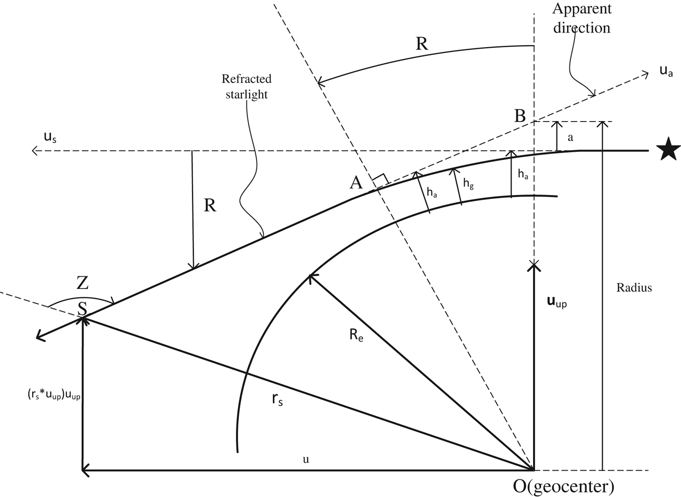
Owing to the variety of atmospheric density, starlight will be refracted when passing through the spherically layered atmosphere (Lair and Duchon, Reference Lair and Duchon1988) as shown in Figure 1. This refraction is more intense if the starlight is closer to the earth's surface.

Figure 1. Geometry of starlight refraction.
Supposing ρ g is the atmospheric density at refraction height h g, the relationship between refraction angle and refraction height can be given in Equation (1) as follows:
 $$R = k(\lambda )\rho _g [2\pi (R_e + h_g )/H_B ]^{1/2} $$
where R is refraction angle, H B is the density scale height, R e is earth radius and k(λ) is the dispersion parameter which is only related to the wavelength λ.
Assuming that atmospheric density changes completely according to the index law, the density at refraction height h g is given as follows:
 $$\rho _g = \rho _0 \exp [ - (h_g - h_0 )/H_B ]$$
where ρ 0 is the atmospheric density at the height h 0.
Because R e is much more than h g, Equation (1) can be simplified as:
 $$R \approx k(\lambda )\rho _g [2\pi R_e /H_B ]^{1/2} $$
Associating Equation (2) with Equation (3), Equation (4) is thus:
 $$h_g = h_0 - H_B \ln (R) + H_B \ln [k(\lambda )\rho _0 (2\pi R_e /H_B )^{1/2} ]$$
The relationship between apparent height h a and refraction height h g is as follows:
 $$h_a = [1 + k(\lambda )\rho _g ]h_g + k(\lambda )\rho _g R_e $$
Associating Equation (4) with Equation (5), Equation (6) is thus:
 $$h_a = h_0 - H_B \ln (R) + H_B \ln [k(\lambda )\rho _0 (2\pi R_e /H_B )^{1/2} ] + R(H_B R_e /2\pi )^{1/2} $$
where H B is the density scale height at 25 km. Therefore, Equation (6) is the measurement model of navigation by starlight refraction at 25 km.
3. DISTURBED ATMOSPHERIC DENSITY MODEL
The measurement model of navigation by stellar refraction is based on the atmospheric density model. The precision of the measurement model is closely related to the accuracy of the atmospheric density (Wang and Ma, Reference Xinlong and Shan2009). Generally, the atmospheric density decreases exponentially with the increase of altitude, and it is influenced by solar activity, time, season, latitude, and geomagnetic activities, especially by season, latitude, and the random changing of atmospheric density. The variety of atmospheric density is defined as the deviation between real density and its standard, expressed as Equation (7):
 $$\delta _\rho = (\rho - \rho _{CT} )/\rho _{CT} $$
where δ ρ is the variety of atmospheric density; ρ is the real density; ρ CT is the standard value.
3.1. Season and Latitude (Ji, Reference Rongfen1995)
The complexity of atmospheric density is mainly manifested in that the atmospheric density differs with time and place. The latitude and season are particularly important factors. During a year, the variety of atmospheric density, pressure, wind speed and other factors at the height from 0 km to 150 km is predictable, within certain limits. The mathematical model of variety of atmospheric density affected by season and latitude is as follows:
 $$\delta _{\rho cm} (H,L,N) = K_0 (H,M) + \sum\limits_{i = 1}^6 {K_i} (H,M)L^i $$
where H is height; L is latitude; M is month. Other coefficients can be calculated as follows:
 $$\eqalign{ & K_0 (H,M) = \delta _{\rho cm1} (H,M) \cr & K_1 (H,M) = 0 \cr & K_2 (H,M) = 0{\cdot}5n_3 \cr & K_3 (H,M) = 0 \cr & K_4 (H,M) = 8{\cdot}729n_1 - 1{\cdot}489n_2 - 1{\cdot}994n_3 \cr & K_5 (H,M) = - 11{\cdot}114n_1 + 2{\cdot}523n_2 + 2{\cdot}203n_3 \cr & K_6 (H,M) = 3{\cdot}538n_1 - 0{\cdot}936n_2 - 0{\cdot}562n_3} $$
In Equation (8), other parameters are as below:
 $$\eqalign{ & n_1 = \delta _{\rho cm2} (H,M) - \delta _{\rho cm1} (H,M) \cr & n_2 = \delta _{\rho cm3} (H,M) - \delta _{\rho cm1} (H,M) \cr & n_3 = - 2u_{cm1} (H,M)[1 + \delta _{\rho cm1} (H,M)\omega _3 r\rho _{CT} /P_{CT} ]} $$
δ ρ cmi(H,M), i=1,2,3, are the default variety of density in corresponding height in Equation (10). They are from three different latitudes: 0°(i=1), 50°(i=2) and 90°(i=3). U cm1(H,M) is the zonal wind on the equator; ω 3 is angular velocity of earth rotation; r is the distance between the position of research and geocenter; ρ CT is standard density; P CT is standard pressure.
The season-latitude component of zonal wind is as follows:
 $$u_{cm} (H,L,M) = - [1/2(1 + \delta _{\rho cm} )\omega _3 r]^*[P_{CT} /(\sin \varphi ^*\rho _{CT} )]^*(\partial \delta _{\rho cm} /\partial \varphi )$$
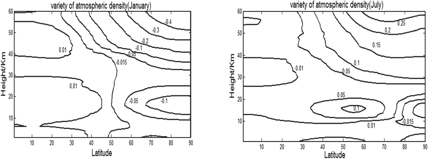
According to Equation (8), the equipotential line of the density variety affected by season and latitude in January and July can be given as shown in Figure 2. In the figure, the axis of abscissa is latitude (0°∼90°N), and the axis of bank is height (0∼60 km). It can be seen that the variety of atmospheric density is affected by latitude and height in different seasons. On the specific height, the variety of atmospheric density will increase with the rising of height. However, there are two heights of equal density at 8 km and 25 km, where the variety of atmospheric density is stable, as shown in Figure 2.
Figure 2. Variety of density affected by season and latitude.
3.2. Random Factors
The variety of atmospheric density affected by random factors reflects its uncertainty. This uncertainty is mainly caused by the changes of solar activity and geomagnetic processes. At the range of the height H⩽100 km, the mathematical model of variety of atmospheric density affected by random factors is as follows:
 $$\eqalign{\delta _{\rho c\pi y} = & X(H,L,M)f_1 (H)f_2 (L) + y(H) \cr & ^*( - 4{\cdot}493^*10^{ - 1} + 1{\cdot}978^*10^{ - 2} \sqrt {T_{CP} - 483{\cdot}92} )} $$
f 1(H) is the characteristic function of density variety at a particular height, it can be given as:
 $$f_1 (H) = a_1 + a_2 \sin [\pi (H - 60)/40]$$
f 2(L) is the characteristic function of density variety on a particular latitude, it can be given as:
 $$f_2 (L) = 0{\cdot}92 + 0{\cdot}08\sin (9L + a_3 )$$
y(H) can be ascertained as below:
 $$y(H) = \left\{ {\hskip -3pt\matrix{ 0 & {\hskip 39pt H \lt 95\; {\rm km}} \cr {3{\cdot}869^*10^{ - 6} (H - 95)^3 + 2{\cdot}632^*10^{ - 4} (H - 95)^2} & {95\, {\rm km} \leqslant H \leqslant 125\, {\rm km}} \cr {2{\cdot}632^*10^{ - 2} (H - 112)} & \hskip 39pt {H \gt 125\, {\rm km}} \cr}} \right.$$
X(H,L,M) is equal to δ ρcπ(H,L,M), which is the limit of density variety. It, at height from 0 km to 150 km and latitude from 0° to 90°, is shown as follows:
 $$\eqalign{\delta _{\rho c\pi} (H,L,M) = & [(1 - \sin (H - 115))/2]^*\{ - 5{\cdot}119^*10^{ - 5} H^2 + 6{\cdot}770^*10^{ - 2} \cr & {\hskip -2pt}+ [q_1 (H,M) ( - 5{\cdot}160^*10^{ - 1} L^3 + 1{\cdot}216L^2 ) + q_2 (H)]\cr &^*\cos ^2 [(\pi |H - H_2 |)/(H_1 - 2|H - H_2 |)]\} \cr & ^*\{ a_1 + a_2 \sin [\pi (H - 60)/40]\} ^*\{ 1 - 0{\cdot}08[1 - \sin (9L + a_3 )]\} \cr & {\hskip -2pt}+ [(1 + \sin (H - 112))/2]^* (H - 112)( - 1{\cdot}182^*10^{ - 2} \cr & {\hskip -2pt}+ 5{\cdot}205^*10^{ - 4} \sqrt {T_{CP} - 483{\cdot}92} )} $$
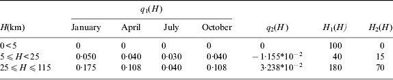
q 1(H), q 2(H), H 1(H), H 2(H) can be chosen from Table 1:
Table 1. Atmospheric parameter (1).

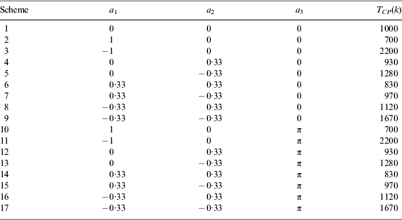
a 1, a 2, a 3 and T CP can be chosen from Table 2:
Table 2. Atmospheric parameter (2).

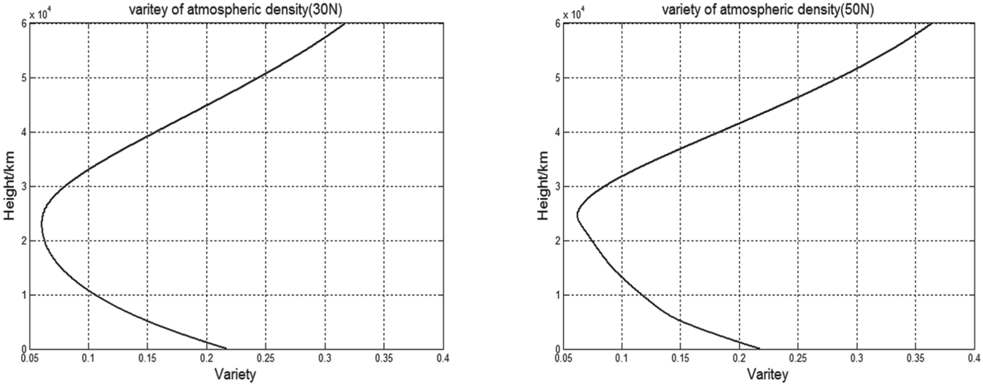
Figure 4 shows the simulation results calculated by Equation (12), where the axis of abscissa is density variety, and the axis of bank is height (0∼60 km). Figure 3 reflects the variety at 30° north latitude and 50° north latitude. It can be seen from the figure that the variety of density affected by random factors can be approximated as a stochastic process that can be simulated by different parameters at different height, latitude, and season. In this random process, there is an obvious interval in which the variety is small. When the height reaches from 20 km to 30 km, the random variety of atmospheric density is slight, and this means that the status is relatively stable in this interval.
Figure 3. Variety of density affected by random factors.
3.3. Establishment and Verification
Usually, the atmospheric density is approximately described as an exponential function of height: ρ=Ae−Bh. The general mathematic model of atmospheric density is as follows:
 $$\rho = 1537{\cdot}3e^{ - 0.1462*h_g} $$
This needs to be modified according to Sections 3.1 and 3.2; Equation (17) is modified, then a new disturbed model of atmospheric density can be obtained as follows:
 $$\rho = 1537{\cdot}3(1 + \delta _{\rho \Sigma} )e^{ - 0.1462*h_g} $$
 $$\delta _{\rho \Sigma} = \delta _{\rho cm} + \delta _{\rho cn} $$
where δ ρΣ is the variety of atmospheric density, including δ ρ cm variety affected by season and latitude and δ ρ cn variety affected by random factors.
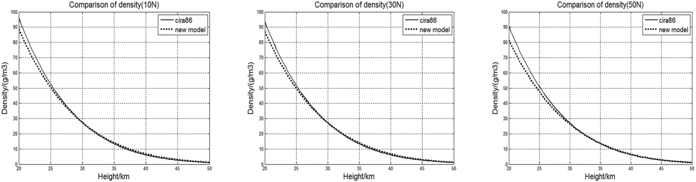
Using the temperature, pressure, wind speed, atmospheric composition and other data on different latitude and geopotential height given by cira1986 (international reference atmosphere), the atmospheric density can be calculated as shown in Figure 4. The solid lines in Figure 4 reflect the average status of atmospheric density at a specific interval of atmospheric pressure. The axis of abscissa is height (20∼50 km), and the axis of bank is atmospheric density (g/m3). The dotted lines in the figure reflect atmospheric density calculated by the model in this paper. As the figures show, the two curves are basically consistent with each other, and the average error is less than 10%. Therefore the new disturbed model of atmospheric density can meet the real situation, and it is practicable.
Figure 4. Comparison of density.
4. ADAPTIVE MEASUREMENT MODEL BASED ON MULTIPLE MODELS SWITCHING
Multiple models adaptive control is used to describe the uncertainty of a system with multiple models, and the corresponding controller is built on each model. The main idea of the multiple models switching approach is that multiple models are built for one system. Furthermore, each model is switched according to the corresponding requirement.
4.1. Fixed Measurement Model
According to the atmospheric density model (Equation (18)), the disturbed measurement model can be obtained by associating Equations (1) and (6). When λ=0·7 μm, k(λ)=2·25*10−7. The refraction model can be obtained through mathematical transformation:
 $$R = 0{\cdot}0338(1 + \delta _{\rho \Sigma} )e^{ - 0{\cdot}1518026*h_g} $$
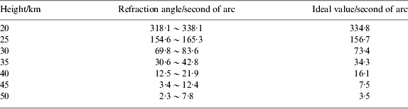
where h g is the refraction height (unit is km), R is refraction angle (unit is second of arc). The variety of refraction angle based on atmospheric density at different height is shown in Table 3.
Table 3. Refraction angle at different height.

The measurement model for corresponding refraction height can be obtained as follows:
 $$h_a = h_g - Hg^*\ln (R) + Hg^*\ln [k(\lambda )\rho _g (2\pi R_e /Hg)^{1/2} ] + R(HgR_e /2\pi )^{1/2} $$
where Hg is the density scale height at refraction height h g; refraction angle R and atmospheric density ρ g changes with refraction height.
Refraction angle decreases as height increases. When the refraction height is beyond 50 km, the refraction angle is lower than the measurement accuracy of the star sensor. Owing to atmospheric brightness, when the refraction height is lower than 20 km, the refraction star is barely captured. Therefore the disturbed measurement models’ range is 20 km to 50 km. According to Equations (20) and (21), fixed measurement models are established at h g=20 km, 25 km, 30 km, 35 km, 40 km, 45 km, and 50 km.
4.2. Multiple Models Switching
According to the seven measurement models established in the range of 20 km ∼50 km in Section 4.1, the appropriate model is picked up automatically on the basis of a switching performance index. The prediction error of the model is defined as:
 $$e_j = h_g - \hat h_g $$
 $\hat h_g $ is the estimated value of refraction height, which can be calculated by the observed refraction angle. The performance index J j(t) is formed by each model's prediction error, while each model could be switched according to which model minimises the performance index. The rationality of this approach lies in that a small prediction error will cause a small concomitant error.
The performance index is as follows:
 $$J_j (t) = \alpha e_j^2 (t) + \beta \int\limits_0^t {e^{ - \theta (t - \tau )} e_j^2 (\tau )d\tau} $$
where α⩾0, β>0, θ>0. Parameters α and β determine the relative importance of transient measurement and long term measurement in the performance index. Parameter θ is a “forgetting” factor, which determines the memory length of the performance index.
4.3. Switching Process
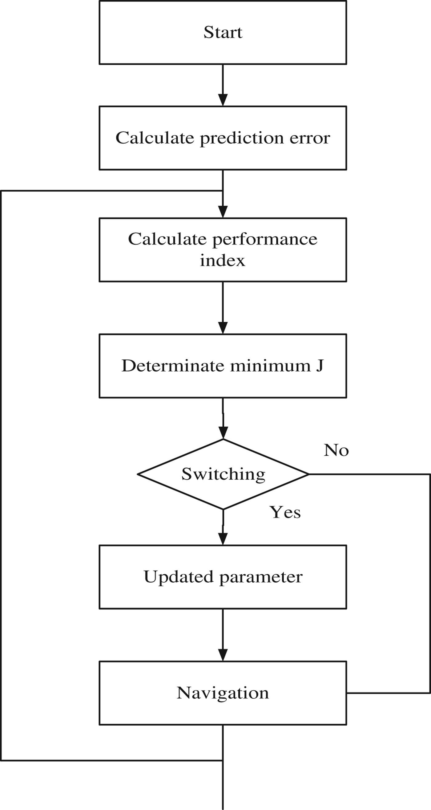
In order to avoid any fast switching, a hysteresis switching algorithm is used. Assuming prediction model I j is selected at time t and J k=min{J i(t)} that J j(T) is not the minimum, if J j(t)⩽J k(t)+δ, model I j will also be selected. But if J j(t)⩾J k(t)+Δ, model I k will be selected, where Δ is a hysteresis factor (Shi et al., Reference Hongrui, Zhihong and Hongtao2004). The switching process is shown in Figure 5.
Figure 5. Switching process of the adaptive model.
The above analysis indicates that when the star sensor captures the refracted starlight at a height of 20 km to 50 km, the system could automatically select the corresponding measurement model. Thus the limitation of the traditional model of a fixed height (25 km) is improved, and the scope of application of the measurement model of stellar refraction expands to the range of 20 km to 50 km. The accuracy and application of navigation by stellar refraction is dramatically improved.
5. SIMULATION
5.1. Dynamic Model
A satellite's movement is affected by many perturbations which include non-spherical earth gravity, solar gravity, lunar gravity, sunlight pressure, atmospheric drag, etc. Compared with the earth gravity, these perturbations are very weak. To model the system states equation, the gravitation and the disturbances in two-order gravity field terms are taken into account in this paper. Other disturbances are equal to process noise with a Gaussian distribution. The state of the satellite can be described by X=[x, y, z, V x, Vy, Vz]T, where x, y, and z are three components of position; V x, Vy and V z are three components of velocity in earth-centred inertial coordinates.
The state equation is described as:
 $$\mathop X\limits^. (t) = f\,(X(t),\user2{} \user1{} t) + \omega (t)$$
 $$f(X(t),\user2{} t) = \left\{ {\matrix{ {\matrix{ {V_x} \cr {V_y} \cr {V_z} \cr}} \cr { - \mu ^*x/r^3 (1 + 3J_2 /2^*(R_e /r)^2 (1 - 5(z/r)^2 )) + \omega _x} \cr { - \mu ^*y/r^3 (1 + 3J_2 /2^*(R_e /r)^2 (1 - 5(z/r)^2 )) + \omega _y} \cr { - \mu ^*z/r^3 (1 + 3J_2 /2^*(R_e /r)^2 (1 - 5(z/r)^2 )) + \omega _z} \cr}} \right.$$
where r is the size of the satellite position vector; J 2 is the disturbances in a two-order gravity field; ω(t)=[0, 0, 0, ω x, ωy, ωz]T is the model noise which can be assumed as a Gaussian white distribution.
5.2. Measurement Equation
The number of refracted stars observed by the satellite is assumed to be 40, distributed uniformly. According to the geometrical relationship as shown in Figure 1, the observation equation can be described as:
 $$h_a = \sqrt {r_s^2 - u^2} + u^*\tan (R) - R_e - \sigma + \nu (t)$$
where u=|r s*us|, r s is the spacecraft position, u s is the true direction of starlight and σ is very small and can be ignored. ν(t) is the measurement noise which also can be assumed as a Gaussian white distribution. ν(t) and ω(t) are independent of each other. Their statistical characteristics are shown as below:
 $$\eqalign{ & E[\omega (k)] = E[\nu (k)] = 0 \cr & E[\omega (k)\omega ^T (\,j)] = Q_k \delta _{kj} \cr & E[\nu (k)\nu ^T (\,j)] = R_k \delta _{kj} \cr & E[\omega (k)\nu ^T (\,j)] = 0} $$
where δ kj is the impulse function.
According to Equation (26), the measurement value of h a can be calculated. The real value of h a needs to be calculated according to Equation (21).
5.3. Results and Analysis Based On UKF
The simulation conditions are as follows: semi-major axis a=7136·635 km; eccentricity e=1·809*10−3; inclination i=65°; right ascension of ascending node Ω=30°; argument of perigee ω=30°; the time passing the perigee t=0. In order to close to a practical application, the filter cycle T is 3 sec. The initial value of the actual state is X(0)=[4·590*106 m, 4·388*106 m, 3·228*106 m, −4·612*103 m/s, 5·014*102 m/s, 5·876*103 m/s]T. The initial value of filtering is X(0|0)=X(0)+[400 m, 400 m, 400 m, 0·8 m/s, 0·8 m/s, 0·8 m/s]T. The covariance matrix of the initial estimate error covariance matrix is P(0|0)=diag((500 m)2, (500 m)2, (500 m)2, (0·2 m/s)2, (0·2 m/s)2, (0·2 m/s)2). The noise covariance matrix of discrete system noise is Q k=E[ωωT]=diag(q 12, q 22, q 12, q 12, q 22, q 12), where q 1=1*10−3 m/s, q 2=2*10−3 m/s. The covariance matrix of measurement noise is R k=E[υυT]=(80 m)2.
5.3.1. Simulation Results
Refraction angle R is the random value in the range of 1″ to 340″. This means refraction height h g is in the range 20 km to 50 km. Based on the multiple models switching algorithm, the adaptive measurement model is automatically selected. Parameter α=1, β=0·1.
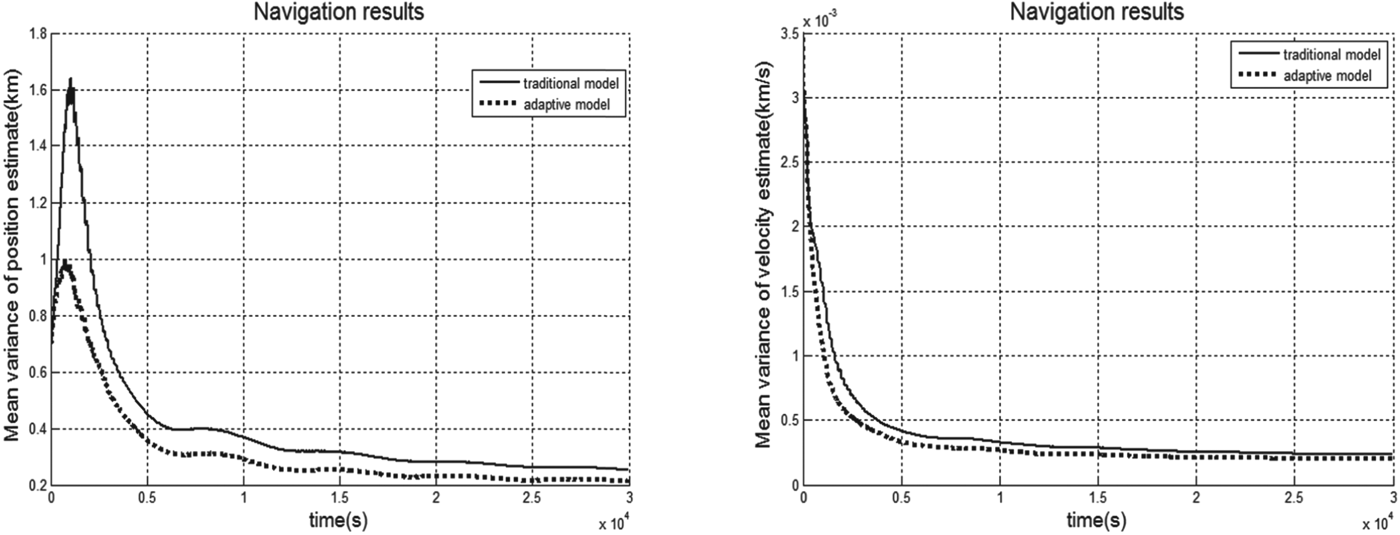
Figure 6 shows a comparison of navigation results between the adaptive measurement model and the traditional model. The solid lines in Figure 6 reflect the navigation results based on the traditional model, and the dotted lines reflect the navigation results based on the adaptive measurement model. If filter cycle T is 3 sec, the variance of the system's position vector is 216·6 m, and the variance of the system's velocity vector is 0·2029 m/s. Comparing the results based on the traditional model, position accuracy is improved by 13·6%, and velocity accuracy is improved by 14% after using the adaptive measurement model.
Figure 6. Comparison of navigation results.
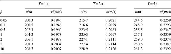
Parameters α and β are two important parameters of the model switching algorithm, which determine the importance of transient measurement and long term measurement in the performance index. The larger β, the more important to long-term measurement is the performance index. If α=1, β could be different values. The navigation results on different filter cycles are shown in Table 4. Character u is the variance of position estimate, and v is the variance of velocity estimate.
Table 4. Navigation results with different parameters.

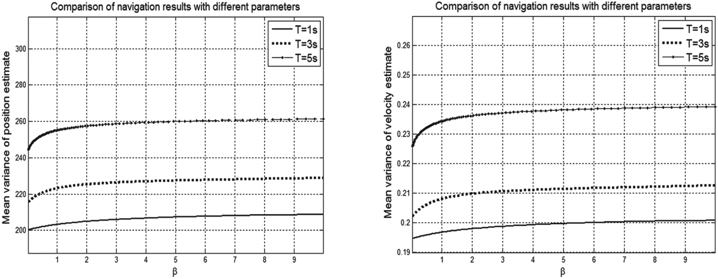
Table 4 shows that the accuracy of navigation decreases with β increasing. The importance of long term measurement in the performance index will increase with increasing β, and this will affect the identification error of the adaptive measurement model. Figure 7 reflects the comparison of navigation results with different parameters. As shown in the figure, the filter cycle has a great influence on the accuracy of navigation. If the filter cycle is larger, accuracy of navigation obviously improves, but this improvement is slow when the filter cycle is smaller.
Figure 7. Comparison of navigation results with different parameters.
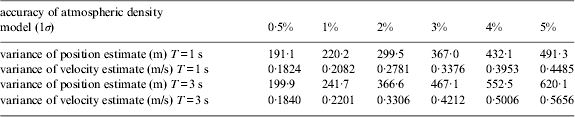
The atmospheric density model has a great influence on the precision of navigation. If the accuracy of the atmospheric density model is 0·5%, 1%, 2%, 3%, 4%, and 5%, the variance of measurement noise can be calculated according to Equation (20) as shown in Table 5.
Table 5. Measurement noise affected by accuracy of atmospheric density model.
Using the variance of measurement noise, the accuracy of navigation influenced by atmospheric density can be obtained as shown in Table 6.
Table 6. Navigation results affected by accuracy of atmospheric density model.

As seen from Table 6, the accuracy of the atmospheric density model is an essential factor affecting the accuracy of navigation by stellar refraction. This effect is more obvious when the filter cycle is larger. If the accuracy of the atmospheric density model is 2%, the navigation results meet the accuracy requirements.
5.3.2. Results Discussion
As can be seen from the results, navigation by stellar refraction can be affected by many factors. The simulation results show that by using the adaptive measurement model, the accuracy of navigation by stellar refraction could be improved. Comparing navigation based on the tradition model, the accuracy can be improved by 14%. Also, the refraction star range captured by star sensor expands from 20 km to 50 km.
α and β are two important parameters of the model switching algorithm which determine the importance of transient measurement and long-term measurement. When the importance of long-term measurement in the performance index is heavier, namely if the β is larger, it is more difficult to achieve high accuracy navigation.
The accuracy of the atmospheric density model is an influential factor on the accuracy of navigation. When the accuracy of atmospheric density model decreased to 1%, the accuracy of navigation results will improve by about 80 m.
6. CONCLUSION
For navigation by stellar refraction, the measurement model is the most crucial element which can decide the results and application of navigation. Due to the uncertainty of atmospheric density, the relationship between refraction angle and refraction height is usually hard to describe. After the study of stellar refraction principles and atmospheric density changes with altitude, latitude, season and other factors, the adaptive measurement model based on multi-model switching is established in this paper, which improves on the limitations of the traditional measurement model.
ACKNOWLEDGEMENT
This work was supported by a grant from the National Natural Science Foundation of China (No. 61074183) and the State Key Program of the National Natural Science Foundation of China (No. 91016004).