


1 Introduction
The exchange of water, solutes and momentum across the interface of sediments and the overlying water plays a significant role in controlling biogeochemical processes in aquatic environments. Examples include hyporheic exchange (Bencala Reference Bencala2000; Wondzell Reference Wondzell2006; Phanikumar et al. Reference Phanikumar, Aslam, Shen, Long and Voice2007; Roche et al. Reference Roche, Li, Bolster, Wagner and Packman2019) and reactive transport processes involving nitrification and denitrification within streams and streambed sediments (Bertuzzo et al. Reference Bertuzzo, Maritan, Gatto, Rodriguez-Iturbe and Rinaldo2007; Gomez-Velez et al. Reference Gomez-Velez, Harvey, Cardenas and Kiel2015; Painter Reference Painter2018). Such interfacial exchange phenomena occur over a wide range of spatial and temporal scales and are affected by a number of key processes and parameters including roughness, bedform, bed porosity and permeability, bed heterogeneity, water flow velocity and unsteadiness (Boano et al. Reference Boano, Harvey, Marion, Packman, Revelli, Ridolfi and Worman2014; Cardenas Reference Cardenas2015).
Fundamental studies of turbulent flow over permeable beds have addressed the effect of varying permeability on canonical turbulent channel flows. These include, for example, experimental studies of Zagni & Smith (Reference Zagni and Smith1976), Kong & Schetz (Reference Kong and Schetz1982), Zippe & Graf (Reference Zippe and Graf1983), Manes, Poggi & Ridolfi (Reference Manes, Poggi and Ridolfi2011) and Kim et al. (Reference Kim, Blois, Best and Christensen2018) and numerical studies of Kuwata & Suga (Reference Kuwata and Suga2016a,Reference Kuwata and Sugab) and Fang et al. (Reference Fang, Han, He and Dey2018). Wall permeability is shown to significantly affect the dynamics and statistics of turbulence, including a higher friction coefficient, a varying von Kármán constant ( $\unicode[STIX]{x1D705}$) dependent on the separation of the penetration depth and the boundary-layer thickness, reduced streamwise velocity fluctuations and augmented wall-normal and spanwise velocity fluctuations due to a relaxation of wall blocking. According to the type of dominant flow processes, the interfacial flow can be separated into three regimes (Suga, Mori & Kaneda Reference Suga, Mori and Kaneda2011; Voermans, Ghisalberti & Ivey Reference Voermans, Ghisalberti and Ivey2017) based on the permeability Reynolds number,
  $Re_{K}=u_{\unicode[STIX]{x1D70F}}\sqrt{K}/\unicode[STIX]{x1D708}$ (where
  $u_{\unicode[STIX]{x1D70F}}$ is the friction velocity,
  $K$ is the permeability and
  $\unicode[STIX]{x1D708}$ is the kinematic viscosity): (i) an effectively impermeable regime (
 $Re_{K}\ll 1$) where attached eddies (Cossu & Hwang Reference Cossu and Hwang2018) dominate the near-wall dynamics, displaying a broad range of turbulent scales, (ii) a highly permeable regime (
 $Re_{K}\gg 1$) where the interface is characterized by a distinct inflection point of the mean velocity and a predictable frequency of coherent motions due to Kelvin–Helmholtz instability and (iii) a transitional regime (
 $Re_{K}\sim o(1)$), where characteristics of both limiting regimes exist. Here, we focus on the momentum transport in a scenario similar to river flows over sand beds, i.e. turbulent water flows over sediments with
  $Re_{K}\sim o(1)$ that allows turbulence to penetrate into the sediment.
A challenge in understanding the mass and momentum transport across the sediment–water interface is associated with the lack of detailed information on the fluid dynamics at the scale of sediment grains, especially near the bed surface. This is due to both the difficulty of experimental measurements at the scale of sediment grains as well as the high cost of numerical simulations to resolve the full spectrum of scales ranging from individual grains to those of ripples, dunes, pool-riffle structures, meanders and the watershed. The wall-normal protuberances formed by individual particles are characterized as bed roughness (or particle roughness). This is to be differentiated from the protuberances of bedforms, which are formed by clusters of particles and are typically orders-of-magnitude larger compared to the length scale associated with the particles.
The bed roughness influences properties of the time-average flow and turbulence over permeable walls (Nikora, Goring & Biggs Reference Nikora, Goring and Biggs1998). Many rough, permeable-bed flow studies focused on the role of permeability using similarly structured sediments that vary in particle size; in this case, it is difficult to separate the effect of roughness from that of permeability, except for cases with very small particle size (Breugem, Boersma & Uittenbogaard Reference Breugem, Boersma and Uittenbogaard2006) or cases where the packing structure is modified inside the bed (Fang et al. Reference Fang, Han, He and Dey2018). Manes et al. (Reference Manes, Pokrajac, McEwan and Nikora2009a) compared permeable and impermeable walls with the same roughness and showed that the penetration of turbulent flows into the porous bed leads to higher flow resistance than an impermeable rough bed. Even in the fully rough regime, the friction factor for the permeable bed increases with Reynolds number.
The understanding of the effect of roughness isolated from that of permeability is much more limited. Padhi et al. (Reference Padhi, Penna, Dey and Gaudio2018) experimentally compared two gravel beds with different bed surface roughnesses. They observed that the bed with streamwise oriented gravels generates significantly higher Reynolds stresses, form-induced stresses and turbulent-kinetic-energy (TKE) flux than the sediment with randomly oriented gravels. Han et al. (Reference Han, Fang, He and Reible2018) conducted direct numerical simulations (DNS) of solute transport on synthesized sediments consisting of regularly packed spheres with a layer of small spheres above to simulate roughness in different regimes of rough-walled turbulence. They found that an increase of roughness Reynolds number disrupts the diffusive layer and causes turbulent motions that more efficiently transport the solute.
While most studies are conducted using regularly packed particles, natural permeable-bed roughness is characterized by random shape, orientation, spacing and arrangement of particles. These irregularities affect the bed roughness and apparent bed permeability and, consequently, could influence strongly the pattern and intensity of turbulence, as well as the transport characteristics across the interface. While the effects of permeability heterogeneity in the bulk of the sediment have been studied in relation to interfacial transport and a few studies emphasized the importance of the uppermost sediment layer on the transport across the interface (Kalbus et al. Reference Kalbus, Schmidt, Molson, Reinstorf and Schirmer2009; Laube, Schmidt & Fleckenstein Reference Laube, Schmidt and Fleckenstein2018), it is not clear how characteristics of the uppermost sediment layer influence the dynamics at the individual grain level as well as the overall exchange of solute mass and momentum. For turbulent flows bounded by impermeable rough walls, surface roughness leads to spatial heterogeneity of the time-averaged fields and, consequently, additional mechanisms of production and transport of TKE and mean momentum that depend sensitively on the roughness texture (Raupach, Antonia & Rajagopalan Reference Raupach, Antonia and Rajagopalan1991; Mignot, Bartheleemy & Hurther Reference Mignot, Bartheleemy and Hurther2009; Yuan & Aghaei Jouybari Reference Yuan and Aghaei Jouybari2018).
The goal of this work is to characterize the detailed effects of different bed roughnesses on aspects of turbulence that are responsible for scalar and momentum transfer, including averaged statistics and flow structural information. Our questions are the following: (i) How different are the roughness characteristics corresponding to regular and random arrangements of sediment grains in the top layer? (ii) How does the bed roughness texture influence the dynamics at the individual grain level and the overall interfacial exchange of mass and momentum? Specifically, how important are the additional, form-induced terms in the momentum and stress balances?
To address the above questions, we perform DNS of fully developed turbulent open-channel flows over grain-resolved permeable beds with an identical bulk permeability (below the interface region) but different roughnesses produced by either random or regular grain arrangements at the bed surface. The Reynolds numbers based on the open-channel height ( $Re_{\unicode[STIX]{x1D70F}}=u_{\unicode[STIX]{x1D70F}}\unicode[STIX]{x1D6FF}/\unicode[STIX]{x1D708}$, where
  $\unicode[STIX]{x1D6FF}$ is the open-channel height) and on the permeability (
 $Re_{K}$) are kept constant. The paper is organized as follows. Section 2 introduces the methodology of the simulations and porous-bed synthesis and compares the two different interfaces generated. Section 3.1 validates the random sediment synthesis by comparing with the experimental measurements of Voermans et al. (Reference Voermans, Ghisalberti and Ivey2017). Section 3.2 compares the turbulence statistics and structure as affected by the differences in the interface. Lastly, § 3.3 discusses implications for the hyporheic exchange mechanisms.
2 Methodology
2.1 Governing equations
The incompressible flow of a Newtonian fluid is governed by the equations of conservation of mass and momentum
 $$\begin{eqnarray}\displaystyle & \displaystyle \frac{\unicode[STIX]{x2202}u_{i}}{\unicode[STIX]{x2202}x_{i}}=0, & \displaystyle\end{eqnarray}$$
 $$\begin{eqnarray}\displaystyle & \displaystyle \frac{\unicode[STIX]{x2202}u_{j}}{\unicode[STIX]{x2202}t}+\frac{\unicode[STIX]{x2202}u_{i}u_{j}}{\unicode[STIX]{x2202}x_{i}}=-\frac{\unicode[STIX]{x2202}P}{\unicode[STIX]{x2202}x_{j}}+\unicode[STIX]{x1D708}\unicode[STIX]{x1D6FB}^{2}u_{j}+F_{j}. & \displaystyle\end{eqnarray}$$
 Here,  $x_{1}$,
  $x_{2}$ and
  $x_{3}$ (or
  $x$,
$x$,  $y$ and
  $z$) are, respectively, the streamwise, wall-normal and spanwise directions, and
  $u_{j}$ (or
  $u$,
$u$,  $v$ and
  $w$) are the velocity components in those directions;
  $P=p/\unicode[STIX]{x1D70C}$ is the modified pressure, where
  $\unicode[STIX]{x1D70C}$ the density. The term
  $F_{j}$ in (2.2) is a body force imposed by an immersed boundary method (IBM) to impose no-slip boundary conditions on the fluid–solid interface. The grain geometry is well resolved by the grid. The IBM is based on the volume-of-fluid approach (Scotti Reference Scotti2006); its detailed implementation and validation are provided in Yuan & Piomelli (Reference Yuan and Piomelli2014a,Reference Yuan and Piomellib). The
  $F_{i}$ values are negligible except in the cells that are cut by the immersed solid boundaries. The simulations are performed using a well-validated code that solves the governing equations (2.1) and (2.2) on a staggered grid using second-order, central differences for all terms, semi-implicit time advancement (with second-order Adams–Bashforth scheme for the wall-normal diffusion term) and MPI parallelization (Keating et al. Reference Keating, Piomelli, Bremhorst and Nešić2004).
Fully developed open-channel flows are simulated with symmetric boundary conditions applied at both top and bottom boundaries of the simulation domain and periodic conditions are applied in  $x$ and
  $z$. A constant pressure gradient is used to drive the flow.
In the sediment, the presence of grains leads to spatial heterogeneity of the time-averaged variables; these time-averaged fluctuations are separated from turbulent fluctuations using the double-averaging (DA) decomposition introduced by Raupach & Shaw (Reference Raupach and Shaw1982),
 $$\begin{eqnarray}\unicode[STIX]{x1D719}(\boldsymbol{x},t)=\langle \overline{\unicode[STIX]{x1D719}}\rangle (y)+\widetilde{\unicode[STIX]{x1D719}}(\boldsymbol{x})+\unicode[STIX]{x1D719}^{\prime }(\boldsymbol{x},t),\end{eqnarray}$$
 where  $\unicode[STIX]{x1D719}$ is an instantaneous flow variable,
  $\langle \unicode[STIX]{x1D719}\rangle$ is the intrinsic spatial average in the
  $(x,z)$-plane,
  $\langle \unicode[STIX]{x1D719}\rangle =1/A_{f}\int _{A_{f}}\unicode[STIX]{x1D719}\,\text{d}A$ (where
  $A_{f}$ is the area occupied by fluid),
  $\overline{\unicode[STIX]{x1D719}}$ is the temporal average,
  $\unicode[STIX]{x1D719}^{\prime }=\unicode[STIX]{x1D719}-\overline{\unicode[STIX]{x1D719}}$ is the instantaneous turbulent fluctuation and
  $\widetilde{\unicode[STIX]{x1D719}}=\overline{\unicode[STIX]{x1D719}}-\langle \overline{\unicode[STIX]{x1D719}}\rangle$ is the form-induced fluctuation. The area averaging carried out in the total area of fluid and solid,
  $A_{o}$, is termed superficial area averaging, denoted by
  $\langle \unicode[STIX]{x1D719}\rangle _{s}=1/A_{o}\int _{A_{f}}\unicode[STIX]{x1D719}\,\text{d}A$; the two averaging approaches satisfy the relation
  $\langle \rangle _{s}=\unicode[STIX]{x1D703}(y)\langle \rangle$, where
  $\unicode[STIX]{x1D703}(y)$ is the plane-averaged porosity at elevation
  $y$,
$y$,
 $$\begin{eqnarray}\unicode[STIX]{x1D703}(y)=\frac{A_{f}(y)}{A_{o}}.\end{eqnarray}$$
 The plane-averaged total drag  $F_{D}(y)$, exerted by the grains on the fluid (including both viscous and pressure drag contributions), is calculated using the IBM body force,
  $\overline{F_{1}}$
 $$\begin{eqnarray}F_{D}(y)=\frac{\unicode[STIX]{x1D70C}}{L_{x}L_{z}}\int _{A_{o}}\overline{F_{1}}(x,y,z)\,\text{d}x\,\text{d}z,\end{eqnarray}$$
 where  $L_{x_{i}}$ is the domain size in
  $x_{i}$. For a detailed explanation of this method, see Yuan & Piomelli (Reference Yuan and Piomelli2014a). The friction velocity,
  $u_{\unicode[STIX]{x1D70F}}$, is calculated based on the maximum value of the total stress, which is the sum of the viscous shear stress, turbulent shear stress and the form-induced shear stress.
2.2 Parameters
The detailed simulation parameters for all cases are listed in table 1. Two types of sediment–water interface (SWI) – regular and random interfaces – are simulated; their definitions are given in § 2.3. Case 1 is used in § 3.1 to validate the synthesis of the random interface generated with experimental data. Cases 2 and 3 share a higher friction Reynolds number than that in Case 1; these two cases are used to compare the effects of different interface geometries on the turbulent flow in § 3.2.

Figure 1. (a) Simulation domain and (b) positions of sediment crest,  $k_{c}$, and zero-plane displacement,
  $d$, defined in § 3.2.1.
Table 1. Summary of simulations.  $\unicode[STIX]{x1D703}_{avg}$ is the average porosity in the bulk of the sediment;
  $D$ is the sphere diameter;
  $H_{s}$ is the sediment depth;
  $L_{x_{i}}$ is the domain size in
  $x_{i}$.

In table 1,  $\unicode[STIX]{x1D703}_{avg}$ is the volume-averaged porosity inside the sediment; its value is kept the same for all cases. The bulk permeability,
  $K$, is estimated using the Kozeny–Carman model (Kozeny Reference Kozeny1927; Carman Reference Carman1937),
 $$\begin{eqnarray}K=\frac{\unicode[STIX]{x1D703}_{avg}^{3}}{180(1-\unicode[STIX]{x1D703}_{avg})^{2}}D^{2},\end{eqnarray}$$
 where  $D$ is the grain diameter. The Kozeny–Carman model has been widely used for multiple types of artificially generated packed beds, for example, by Voermans et al. (Reference Voermans, Ghisalberti and Ivey2017) for a random packing of spheres and by Fang et al. (Reference Fang, Han, He and Dey2018) for periodic arrays of spheres. The elevation of
  $y=0$ is chosen at the sediment crest, for ease of simulation domain set-up. However,
  $y=0$ is not used as the virtual origin of the
  $y$ axis for comparison of flow statistics. Instead, the virtual origin is chosen at the zero-plane displacement,
  $-d$, which is obtained by fitting the DA velocity to the logarithmic law (shown in § 3.2);
  $H_{s}$ is the sediment depth measured from the sediment crest to the bottom boundary of the simulation domain. Figure 1(a,b) shows the simulation domain and the relation between various lengths and the
  $y$ axis.
The domain sizes for Case 1 in the  $x$ and
  $z$ directions are
  $12\unicode[STIX]{x1D6FF}$ and
  $6\unicode[STIX]{x1D6FF}$, respectively. For Cases 2 and 3 with higher
  $Re_{\unicode[STIX]{x1D70F}}$ values, smaller domain sizes are used. Such domain sizes are considered sufficiently large for the following reasons. (i) The streamwise and spanwise two-point autocorrelations of the streamwise turbulent velocity fluctuations, calculated at
  $y\leqslant 0.5\unicode[STIX]{x1D6FF}$, fall below 0.1 at half the domain length or width for all cases. (ii) The domain is sufficient for the sediment domains to contain 2000–2500 randomly distributed grains to produce statistically converged single-point and two-point turbulent flow statistics. A test is performed for Case 3 with a domain size twice as large in both
  $x$ and
  $z$, which yields similar results. (iii) The sediment depth,
  $H_{s}$, is much larger than the penetration depth of turbulence into the sediment, as shown in § 3.2. The total simulation time for each case is at least
  $T=25\unicode[STIX]{x1D6FF}/u_{\unicode[STIX]{x1D70F}}$ after the transient.
The number of grid points is  $1024(x)\times 380(y)\times 512(z)$ for Case 1 and
  $1536(x)\times 478(y)\times 768(z)$ for Cases 2 and 3. For Cases 2 and 3, we have verified that coarsening
  $\unicode[STIX]{x0394}x_{i}^{+}$ twofold does not noticeably affect the results shown in this paper. Here, superscript
  $+$ indicates normalization by the viscous length scale,
  $\unicode[STIX]{x1D6FF}_{\unicode[STIX]{x1D708}}=\unicode[STIX]{x1D708}/u_{\unicode[STIX]{x1D70F}}$. Uniform spacing of grids is used in
  $x$ and
  $z$;
$z$;  $\unicode[STIX]{x0394}x=\unicode[STIX]{x0394}z$. The grain geometry is resolved by 36 grid points along each direction in Case 1 and 50 grid points in Cases 2 and 3. In the
  $y$ direction, 120 grid points are used to refine the grid within one diameter distance below the crest; deeper inside the sediment, uniform
  $\unicode[STIX]{x0394}y$, the same as the grid size in
  $x$ and
  $z$, is used. Above the crest, the
  $y$ grid is stretched with finer resolution close to the interface. The minimum vertical grid spacing
  $\unicode[STIX]{x0394}y_{min}^{+}$ in wall units is 1.5 for Case 1 and 0.19 for Cases 2 and 3. The maximum
  $\unicode[STIX]{x0394}y^{+}$ is 5.3 for Case 1 and 4.2 for Cases 2 and 3.
To provide further evidence that the resolution of 50 grid points per diameter captures well the velocity distribution and forces produced by the spheres, we conducted another simulation of a uniform flow past a single sphere with a set-up similar to Mittal et al. (Reference Mittal, Dong, Bozkurttas, Najjar, Vargas and Von Loebbecke2008) and compared the results to the experimental measurements of Taneda (Reference Taneda1956). Two values of the Reynolds number based on grain diameter,  $DU/\unicode[STIX]{x1D708}$ (where
  $U$ is the uniform undisturbed velocity), of 75 and 100 were used. These values are similar to or higher than the Reynolds number experienced by the spheres near the interface in this work. Results (not shown) quantify the difference between our DNS and the experimental results as 1 %–4 % for the flow characteristics (separation angle, recirculation bubble size and recirculation centre location) and 1 %–1.5 % for the drag force. The comparison gives confidence that the results herein, especially the local mean shear layers (important for turbulence production) and the drag force (important for form-induced stress production (Raupach & Shaw Reference Raupach and Shaw1982)) are well captured by the spatial resolution.
2.3 Synthesis of porous beds
Numerical studies of permeable walls usually employ idealized models characterized by regular packing of grains and a constant bed height due to their easy implementation. Examples include a Cartesian grid of cubes used by Breugem & Boersma (Reference Breugem and Boersma2005), a regular packed bed of Breugem et al. (Reference Breugem, Boersma and Uittenbogaard2006) or a simple cubic packing of spheres used in Stoesser, Frohlich & Rodi (Reference Stoesser, Frohlich and Rodi2007) and Fang et al. (Reference Fang, Han, He and Dey2018). Numerical approximations of natural sediments were constructed by, for example, Stubbs, Stoesser & Bockelmann-Evans (Reference Stubbs, Stoesser and Bockelmann-Evans2018), who used a computer-aided design model to design and manufacture an artificial gravel riverbed to approximate a natural bed for both experimental and numerical studies. Here, we implement a different approach based on molecular dynamics (MD) simulations, which are widely applied in flows through porous media with applications in materials science (Khirevich Reference Khirevich2011; Amadio Reference Amadio2014). The simulations are carried out using the open-source code LAMMPS (Plimpton Reference Plimpton1995) to generate sediments composed of randomly packed, monodisperse hard spheres. The process of pouring hard spheres into a tank is simulated; this process is designed to reproduce the sediment used in the experimental studies of Voermans et al. (Reference Voermans, Ghisalberti and Ivey2017) (henceforth referred to as VGI17). Details of the MD simulations are included in appendix A.
Two types of distribution of the sphere-centre locations of the uppermost-layer spheres are generated: (i) regular distribution in  $(x,z)$ with constant height,
  $y$, called a regular interface, and (ii) random values in both
  $(x,z)$ and
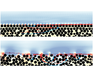
  $y$ directions, called a random interface. Below the interface, sediments with both types of interface are synthesized using a random sphere distribution that is statistically similar. The total number of spheres are 2633, 2351 and 2116, for Cases 1, 2 and 3, separately. Figure 2 compares the sphere distributions in Cases 2 and 3; the difference at the top of the sediments is apparent. These characteristics of the interface can also be expressed in terms of the mean and variance of the permeability in the uppermost sediment layer as well as the correlation length scales in the
  $x$ and
  $z$ directions (§ 2.4).

Figure 2. Synthesized sediment beds coloured by  $y/\unicode[STIX]{x1D6FF}$ with (a) regular and (b) random interfaces.
2.4 Geometrical comparison of the two interface types

Figure 3. Wall-normal profiles of plane-averaged porosity profile for regular (- - - -) and random (——) interfaces.
The characteristics of the grain distributions in Cases 2 and 3 are compared. First, the plane-averaged porosity profiles along the vertical direction are shown in figure 3. In the interface region ( $y\approx 0$), the random interface yields monotonically decreasing porosity with decreasing
  $y$, with an inflection point as observed in VGI17. In comparison, the regular sediment yields a different pattern, with large-amplitude fluctuations. This is due to the constant sphere height in the uppermost layer. The vertically averaged porosity inside the sediment is the same between the two cases.

Figure 4. Bed surface height fluctuations for the (a) regular and (b) random interfaces. (c) Autocorrelation of height fluctuations and Taylor micro-scales.
Table 2. Flow parameters for Cases 2 and 3.  $\unicode[STIX]{x1D6FF}_{b}$ and
  $\unicode[STIX]{x1D6FF}_{p}$ are Brinkman-layer thickness and Reynolds-stress penetration depth, both measured from
  $y=-d$;
  $\unicode[STIX]{x1D6FF}_{b}^{\ast }$ and
  $\unicode[STIX]{x1D6FF}_{p}^{\ast }$ are the same lengths measured from crest;
  $K^{\ast }$ is apparent permeability.

To characterize the positioning of the sediment grains located in the vicinity of the interface, we define the local bed surface height,  $h(x,z)$, as the highest sphere-surface elevation at each
  $(x,z)$ location. Note that this is different from using the sediment-grain centre height (which would yield constant height distribution for the regular interface). Since the penetration depths are within one sphere diameter, as shown later in table 2, only sphere surfaces within one sphere diameter distance below the crest are considered in calculating
  $h(x,z)$. The number of top-layer spheres identified in this way is 900 for the regular interface (Case 2) and 632 for the random interface (Case 3). The sediment-height fluctuations,
  $h^{\prime }(x,z)$, are defined as the deviations of the local height value
  $h(x,z)$ from its plane-averaged value. Figure 4(a,b) compare
  $h^{\prime }(x,z)$ distributions in Cases 2 and 3, normalized by
  $\unicode[STIX]{x1D6FF}$. Interpolation is carried out to show a smooth variation for demonstration. The magnitude of
  $h(x,z)$ fluctuations can be characterized by the root-mean-square value of
  $h^{\prime }$,
  $\unicode[STIX]{x1D70E}_{h}$. The
  $\unicode[STIX]{x1D70E}_{h}^{+}$ values are 17 and 23 for Cases 2 and 3, respectively. The horizontal distribution of
  $h^{\prime }(x,z)$ is characterized here by a Taylor micro-scale,
  $\unicode[STIX]{x1D706}$, determined from a polynomial fit of the two-point autocorrelation
  $R_{x}$ of
  $h^{\prime }$, similar to the method used by Padhi et al. (Reference Padhi, Penna, Dey and Gaudio2018). Here,
  $R_{x}$ is calculated as
 $$\begin{eqnarray}R_{x}=\frac{1}{A_{o}}\int _{x,z}h^{\prime }(x,z)h^{\prime }(x+r_{x},z)\,\text{d}A,\end{eqnarray}$$
 where  $r_{x}$ is the separation length in
  $x$. Figure 4(c) shows that
  $\unicode[STIX]{x1D706}^{+}$, estimated using the two-point correlation with streamwise separation, is 15 and 28 for Cases 2 and 3, respectively. The significant difference in roughness length scales affects the apparent permeability in the uppermost sediment layer, as shown in § 3.3.1. The random interface is more heterogeneous with a larger mean and variance of the apparent permeability, although the permeability in the bulk of the sediment is the same.

Figure 5. Probability density function of bed height fluctuations for (a) regular and (b) random interfaces.
The probability density functions of  $h^{\prime }(x,z)$ are shown in figure 5. Case 2 (regular) gives a highly skewed probability distribution with a skewness of
  $-2.5$ and a kurtosis of 8.7, while Case 3 (random) displays a less skewed but still asymmetric distribution with a skewness of
  $-0.075$ and kurtosis of 1.9. The skewness and a kurtosis of Case 3 are well within the ranges for gravel beds summarized in Nikora et al. (Reference Nikora, Goring and Biggs1998), confirming that the interface is random. These observations show that the major differences between the sediment surfaces in Cases 2 and 3 are the larger wall-normal and horizontal length scales for the random case. These lengths are small compared to the grain size (
 $D^{+}\approx 70$); thus, such height fluctuations are considered as roughness, instead of bedform, whose length scales are much larger than the grain scale. We have also verified that different realizations of the random interface (obtained from separate MD simulations) share similar geometrical characteristics of the sediment surface. For example, another realization of the sediment in Case 1 gives matching values of
  $\unicode[STIX]{x1D70E}_{h}/D$ and
  $\unicode[STIX]{x1D706}/D$ within 1 % difference.
3 Results
3.1 Validation of sediment synthesis
To test how the random interface mimic sediment beds in natural and laboratory settings, we compare Case 1 with the measurements of Case L12 from VGI17. The present values of  $\unicode[STIX]{x1D703}=0.41$ and
  $Re_{K}=2.56$ match those in VGI17 and fall in the range in real aquatic systems. To be consistent with VGI17, in this section we define the location of
  $y=0$ to be the location where
  $\unicode[STIX]{x2202}^{2}\unicode[STIX]{x1D703}/\unicode[STIX]{x2202}y^{2}=0$. Note that for the rest of this paper,
  $y=0$ is defined at the sediment crest (while the virtual origin is chosen as
  $y=-d$ for statistics comparison, as discussed in § 3.2).

Figure 6. Comparison of (a) mean velocity and (b–d) streamwise, wall-normal and shear components of the Reynolds-stress tensor. ○ Experiment, —— DNS.
The comparison of the mean velocity profile  $U=\langle \overline{u}\rangle$ normalized by the DA free-surface (or channel half-height) flow velocity,
  $U_{\unicode[STIX]{x1D6FF}}$, is shown in figure 6(a). Excellent agreement is obtained. Figure 6(b–d) shows the comparison of the turbulence intensities normalized by
  $u_{\unicode[STIX]{x1D70F}}$. Very good agreement is obtained and the slight differences in the outer layer (
 $y/\unicode[STIX]{x1D6FF}\geqslant 0.3$) are probably due to the fact that the flow in the experiment at the measurement station is not a fully developed open-channel flow, but resembles a spatially developing boundary-layer flow.

Figure 7. Comparison of (a) streamwise, (b) wall-normal and (c) shear components of the form-induced stress tensor. ○ Experiment, —— DNS. Black lines represent the values spatially averaged over the entire horizontal plane; grey lines emulate the sampling used in the experiment.
The intensities of the form-induced fluctuations normalized by  $u_{\unicode[STIX]{x1D70F}}$ are compared in figure 7. Relatively large discrepancies are found between the present DNS and the experimental measurements. This is at least partially attributed to a difference in the sampling size. The sizes of the sediment domains are similar between the present DNS and the experiment; however, for the DNS, the spatial averaging is carried out throughout the entire
  $(x,z)$ domain, while the spatial averaging in the experiment was carried out over six lateral measurement frame positions at one streamwise location only. The form-induced stresses have been found to be highly sensitive to the interface geometry (Nikora et al. Reference Nikora, Goring, McEwan and Griffiths2001; Fang et al. Reference Fang, Han, He and Dey2018). If we mimic the experimental sampling protocol by applying the spanwise averaging procedure at six uncorrelated spanwise locations and then repeating the procedure for different streamwise locations using the DNS data, we obtain a family of curves whose envelope provides an indication of the level of uncertainty in the experimental measurements. Such a family of curves is shown by the grey lines in figure 7 while the black solid lines denotes DNS results using spatial averaging over the entire domain. The VGI17 data points fall within the scatter.
In addition to the uncertainties arising due to sampling size, subtle differences in details of the sphere distribution near the interface may also contribute to discrepancies in form-induced velocity fluctuations. However, since the detailed grain-distribution characteristics are not available from VGI17, we consider the synthesized sediment sufficiently ‘realistic’ as it reproduces quantitatively the turbulence statistics and matches qualitatively the form-induced fluctuations. In comparison, a sediment with a regular interface may yield flow statistics that are drastically different as described in § 3.2.
3.2 Effects of interface irregularity on flow statistics
In this section, Cases 2 and 3 are compared to understand the effects of interface characteristics on turbulence statistics and structure.
3.2.1 DA velocity and friction

Figure 8. (a) Diagnostic function for fitting the logarithmic profile and (b) DA velocity profiles for regular (– – –) and random (——) interfaces; - - - (red) fitted logarithmic profiles.
The location of the zero-plane displacement,  $d$, and the von Kármán constant,
  $\unicode[STIX]{x1D705}$, of the wall-bounded flow are determined by fitting the streamwise DA velocity profile to the logarithmic law,
 $$\begin{eqnarray}U^{+}=\frac{1}{\unicode[STIX]{x1D705}}\log (y+d)^{+}+B,\end{eqnarray}$$
 where  $B$ is the intercept of the logarithmic profile. The fitting procedure is similar to the method used by Breugem et al. (Reference Breugem, Boersma and Uittenbogaard2006) and Suga et al. (Reference Suga, Matsumura, Ashitaka, Tominaga and Kaneda2010) and is demonstrated in figure 8(a). The fitted velocity profiles are shown in figure 8(b). The fitted values of
  $\unicode[STIX]{x1D705}$ and
  $d$ are listed in table 2; these values are close to the results (
 $\unicode[STIX]{x1D705}=0.31{-}0.32$ and
  $d/\unicode[STIX]{x1D6FF}=0.06{-}0.1$) reported by Breugem et al. (Reference Breugem, Boersma and Uittenbogaard2006), Suga et al. (Reference Suga, Matsumura, Ashitaka, Tominaga and Kaneda2010) and Manes et al. (Reference Manes, Poggi and Ridolfi2011) at similar
  $Re_{K}$. It is well established that
  $\unicode[STIX]{x1D705}$ for turbulence bounded by a porous wall is smaller than the corresponding value for an impermeable wall, which is usually within
  $5\,\%$ of 0.41 for both smooth and rough walls. Despite sharing similar
  $\unicode[STIX]{x1D705}$ values, Cases 2 and 3 differ significantly in
  $d$. Recalling that
  $d$ is measured from the sediment crest height, the higher
  $d$ in Case 3 is probably due to the larger variance in local sediment heights associated with the random interface. In the following plots we offset
  $y$ by the amount of
  $d$ to effectively collapse the logarithmic regions between the two cases.

Figure 9. DA velocity along  $y$ in linear scaling for regular (– – –) and random (——) interfaces. Inset magnifies the distribution at
  $y\approx -d$.
The DA velocity profiles in linear scaling (figure 9) show the differences in the velocities near the interface. The velocity in the vicinity of the regular interface is negative with a small magnitude. This can be related to the organized recirculation regions induced by each sphere at the top layer (discussed in § 3.2.3). This is an important observation with implications for interfacial exchange of solutes. Also, simpler models, especially those that ignore inertial effects, may not be able to capture these features. Such a flow pattern is also described in the conceptual model of Pokrajac & Manes (Reference Pokrajac and Manes2009). For lower  $y$, the velocity decreases and eventually reaches a constant, positive value inside the sediment. For the random interface, the velocity variation is monotonic. Both velocity profiles exhibit an inflection point near the sediment crest, consistent with observations of Manes et al. (Reference Manes, Poggi and Ridolfi2011), Voermans et al. (Reference Voermans, Ghisalberti and Ivey2017).
The depth of shear-layer penetration,  $\unicode[STIX]{x1D6FF}_{b}$, is defined as the distance from the
  $y=-d$ to the
  $y$ location separating the constant-velocity region in the bed and the shear layer above;
  $\unicode[STIX]{x1D6FF}_{b}$ is also referred to as the Brinkman-layer thickness. Here,
  $\unicode[STIX]{x1D6FF}_{b}$ is calculated in the same way as in Voermans et al. (Reference Voermans, Ghisalberti and Ivey2017),
  $\langle \overline{u}\rangle _{y+d=-\unicode[STIX]{x1D6FF}_{b}}=0.01(U_{i}-U_{p})+U_{p}$, where
  $U_{i}$ is the DA velocity at
  $y=-d$ and
  $U_{p}$ is the constant velocity deep in the sediment;
  $\unicode[STIX]{x1D6FF}_{b}$ is the penetration depth measured from
  $y=-d$. The value measured from the crest,
  $\unicode[STIX]{x1D6FF}_{b}^{\ast }=\unicode[STIX]{x1D6FF}_{b}+d$, for the two cases is shown in table 2, equalling
  $0.138\unicode[STIX]{x1D6FF}$ (regular case) and
  $0.165\unicode[STIX]{x1D6FF}$ (random case). They are of the same order as the grain diameter, as also observed by Goharzadeh, Khalili & Jørgensen (Reference Goharzadeh, Khalili and Jørgensen2005).
The friction coefficient is defined as
 $$\begin{eqnarray}C_{f}=2\left(\frac{u_{\unicode[STIX]{x1D70F}}}{U_{\unicode[STIX]{x1D6FF}}}\right)^{2}.\end{eqnarray}$$
 Table 2 shows that the friction coefficient on the random interface is 70 % higher than the regular one. A higher  $C_{f}$ for the random interface is expected as the larger interface length scales (
 $\unicode[STIX]{x1D70E}_{h}^{+}$ and
  $\unicode[STIX]{x1D706}^{+}$) lead to higher total drag, similar to the effects of an impermeable wall with a larger roughness length scale.
3.2.2 Turbulent fluctuations
Figure 10(a,b) compares the Reynolds-stress tensor and its anisotropy between the two cases. The Reynolds-stress anisotropy tensor is defined as
 $$\begin{eqnarray}b_{ij}=\frac{\langle \overline{u_{i}^{\prime }u_{j}^{\prime }}\rangle }{\langle \overline{u_{k}^{\prime }u_{k}^{\prime }}\rangle }-\frac{\unicode[STIX]{x1D6FF}_{ij}}{3}.\end{eqnarray}$$
 It is shown that Townsend’s wall-similarity hypothesis for a wall-bounded flow applies to the outer layer ( $y/\unicode[STIX]{x1D6FF}>0.2$). As
  $y$ decreases from the sediment crest, for both cases all components of the Reynolds-stress tensor are damped rapidly, together with a decrease of tensor anisotropy. In the interface region, the random interface results in a lower Reynolds-stress anisotropy with a higher fraction of TKE residing in
  $v^{\prime }$ and
  $w^{\prime }$ motions.

Figure 10. Components of (a) the Reynolds-stress tensor and (b) the anisotropy tensor for regular (– – –) and random (——) interfaces.

Figure 11. Contours of instantaneous  ${u^{\prime }}^{+}$ in the
  $(x,z)$ plane at the respective
  $\langle \overline{u^{\prime 2}}\rangle$-peak elevations for the (a) regular and (b) random interfaces.
The more isotropic turbulence near the random interface is linked to the augmented disturbance from the sediment obstruction to the near-wall turbulent coherent structures. Figure 11 compares the contours of  ${u^{\prime }}^{+}$ at the respective locations of the
  $\langle \overline{u^{\prime 2}}\rangle$ peaks in the two cases. The low-speed streaks near the random interface are significantly shorter in wall units than those near the regular interface due to the physical blockage from the spheres serving as roughness elements.
The penetration depth of turbulent shear stress into the bed,  $\unicode[STIX]{x1D6FF}_{p}$, is obtained from
  $\langle \overline{u^{\prime }v^{\prime }}\rangle _{y=-\unicode[STIX]{x1D6FF}_{p}}=0.01\langle \overline{u^{\prime }v^{\prime }}\rangle _{i}$, following Voermans et al. (Reference Voermans, Ghisalberti and Ivey2017), and shown in table 2;
  $\langle \overline{u^{\prime }v^{\prime }}\rangle _{i}$ is the value of
  $\langle \overline{u^{\prime }v^{\prime }}\rangle$ at
  $y=-d$;
  $\unicode[STIX]{x1D6FF}_{p}^{\ast }$ is the same depth measured from the crest. The flow over the random interface gives significantly deeper turbulence penetration, as shown by a 47 % higher
  $\unicode[STIX]{x1D6FF}_{p}^{\ast }$ and 20 % higher
  $\unicode[STIX]{x1D6FF}_{p}$ compared to the regular interface.

Figure 12. Integral length scales of  $u^{\prime }$ motions along the streamwise direction for regular (– – –) and random (——) interfaces.
To quantitatively compare turbulent scales, the integral length scales are shown in figure 12. It is defined as
 $$\begin{eqnarray}L_{ij,x_{k}}(y)=\int _{0}^{\infty }R_{ij}(y,\unicode[STIX]{x0394}r_{k})d(\unicode[STIX]{x0394}r_{k}),\end{eqnarray}$$
where
 $$\begin{eqnarray}R_{ij}(y,\unicode[STIX]{x0394}r_{k})=\frac{\langle \overline{u_{i}^{\prime }(y,x_{k})u_{j}^{\prime }(y,x_{k}+\unicode[STIX]{x0394}r_{k})}\rangle }{\unicode[STIX]{x1D70E}_{u_{i}}(y)\unicode[STIX]{x1D70E}_{u_{j}}(y)}\end{eqnarray}$$
 (no summation over repeated indices). Here,  $\unicode[STIX]{x0394}r_{k}$ is the separation along the
  $x_{k}$ direction and
  $\unicode[STIX]{x1D70E}_{u_{i}}(y)$,
  $\unicode[STIX]{x1D70E}_{u_{j}}(y)$ are the root-mean-square of turbulent fluctuations. The integration is carried out to the value of
  $\unicode[STIX]{x0394}r_{k}$ at which the correlation coefficient first crosses 0.3. A threshold value between 0.3 and 0.5 is usually used to calculate the integral lengths from two-point correlation coefficients (see, for example, Krogstad & Antonia (Reference Krogstad and Antonia1994), Christensen & Wu (Reference Christensen and Wu2005) and Volino, Schultz & Flack (Reference Volino, Schultz and Flack2011)). It has been checked that varying this threshold from 0.2 to 0.5 would not noticeably affect the comparison. It is shown that, for the random interface, at
  $y=-d$ the coherent motions are more extensive in
  $x$ due to a deeper flow penetration. At the sediment crest, however, the coherent motions are noticeably shorter in
  $x$ for the random interface, due to the disturbances of the larger roughness height.
Farther away from the interface ( $(y+d)/\unicode[STIX]{x1D6FF}>0.15$), the difference in the
  $x$ integral length between the two cases systematically increases with
  $y$, indicating a lack of Townsend’s wall-similarity hypothesis for this flow quantity. One reason is the relatively high roughness. Jiménez (Reference Jiménez2004) has proposed that Townsend’s hypothesis applies when the roughness height is less than
  $0.02\unicode[STIX]{x1D6FF}$. In the present study, the roughness height (measured from
  $y=-d$) is at least
  $0.06\unicode[STIX]{x1D6FF}$. Another possible reason is the limited Reynolds number used in the present DNS. The experimental study of Krogstad & Antonia (Reference Krogstad and Antonia1994) showed a lack of similarity in the outer layer
  $L_{11}$ in
  $x$ between a smooth-wall and a rough-wall turbulent boundary-layer flow. However, a repeated experiment of boundary layer flows by Krogstad & Efros (Reference Krogstad and Efros2012) at a higher Reynolds number indicated reduced discrepancy in the outer layer
  $L_{11}$.
3.2.3 Form-induced fluctuations

Figure 13. Components of the form-induced stress tensor: (a) streamwise, (b) wall-normal and (c) spanwise components, for regular (– – –) and random (——) interfaces.

Figure 14. (a) Time-averaged streamlines for the regular interface. (b) Streamlines on Slice A ( $(x,y)$ plane across the crests of the grains). (c) Streamline distribution on Slice B (
 $(x,y)$ plane across the valley between two rows of grains). Dashed lines indicate
  $y=-d$.

Figure 15. (a) Time-averaged streamlines for the random interface. Panels (b) and (c) show streamlines on two  $(x,y)$ planes, Slice C and Slice D. Dashed lines indicate
  $y=-d$.
The form-induced stresses are shown in figure 13. The peak values of all components are much smaller than the corresponding Reynolds stresses, consistent with observations of Manes et al. (Reference Manes, Pokrajac, McEwan and Nikora2009b), Voermans et al. (Reference Voermans, Ghisalberti and Ivey2017) and Fang et al. (Reference Fang, Han, He and Dey2018). The streamwise form-induced stress near the regular interface region is concentrated in a narrower layer near the crest elevation with a much higher peak value. This is due to the vertical alignment of the wake regions of the grains, as shown in figure 14(b,c). Large values of  $\langle \widetilde{u}^{2}\rangle$ are found in the troughs of the top sediment surface and in the wake regions of the surface protuberances. Since these regions are located in a narrow layer near the crest, the distribution of
  $\langle \widetilde{u}^{2}\rangle$ is narrower with a larger peak. In contrast, figure 15 shows that, for the random interface, the mean recirculation regions can reach much larger sizes and that the penetration of the time-mean flow is much deeper. In addition,
  $\langle \widetilde{v}^{2}\rangle$,
  $\langle \widetilde{w}^{2}\rangle$ and
  $\langle \widetilde{u}\,\widetilde{v}\rangle$ are higher near the random interface. This may be explained by the higher spatial variation of
  $\widetilde{u}$ associated with the disordered blockage, which leads to more intense
  $\widetilde{v}$ and
  $\widetilde{w}$ through continuity.

Figure 16. Shear stresses for cases with (a) regular and (b) random interfaces: - - - (blue) Reynolds shear stress, – – – viscous shear stress and —— (red) form-induced shear stress.
To analyse the importance of form-induced stresses to the mean momentum balance, we compare the magnitudes of the various shear stresses in figure 16. For the regular interface, the form-induced shear stress is negligible; the viscous shear stress contributes significantly to the total shear stress at the sediment crest. However, for the random interface the viscous shear is weaker due to the milder DA velocity gradient associated with the thicker shear layer; a much stronger form-induced stress is present.
It is important to note that, in the vicinity of the random interface, the form-induced shear stress reaches a similar magnitude of the Reynolds shear stress (figure 16b). The fact that the form-induced stress potentially affects the DA velocity near the interface and that it strongly depends on the interface geometry calls for a systematic study of the generation of the form-induced stresses; however, this is beyond the scope of the present work.
3.2.4 Reynolds-stress budgets
The budget equations of the normal Reynolds stresses,  $\langle \overline{u_{\unicode[STIX]{x1D6FC}}^{\prime 2}}\rangle _{s}$, can be written as (Raupach & Shaw Reference Raupach and Shaw1982; Mignot et al. Reference Mignot, Bartheleemy and Hurther2009; Yuan & Aghaei Jouybari Reference Yuan and Aghaei Jouybari2018)
 $$\begin{eqnarray}\displaystyle 0 & = & \displaystyle \underbrace{-2\langle \overline{u_{\unicode[STIX]{x1D6FC}}^{\prime }v^{\prime }}\rangle _{s}\frac{\unicode[STIX]{x2202}\langle \overline{u}_{\unicode[STIX]{x1D6FC}}\rangle }{\unicode[STIX]{x2202}y}}_{P_{s}}\underbrace{-2\langle \overline{u_{\unicode[STIX]{x1D6FC}}^{\prime }u_{j}^{\prime }}\rangle _{s}\left\langle \frac{\unicode[STIX]{x2202}\widetilde{u}_{\unicode[STIX]{x1D6FC}}}{\unicode[STIX]{x2202}x_{j}}\right\rangle }_{P_{m}}\underbrace{-2\left\langle \widetilde{u_{\unicode[STIX]{x1D6FC}}^{\prime }u_{j}^{\prime }}\frac{\unicode[STIX]{x2202}\widetilde{u}_{\unicode[STIX]{x1D6FC}}}{\unicode[STIX]{x2202}x_{j}}\right\rangle _{s}}_{P_{w}}\underbrace{-\left\langle \frac{\unicode[STIX]{x2202}}{\unicode[STIX]{x2202}x_{j}}\widetilde{u_{\unicode[STIX]{x1D6FC}}^{\prime }u_{\unicode[STIX]{x1D6FC}}^{\prime }}\widetilde{u}_{j}\right\rangle _{s}}_{T_{w}}\nonumber\\ \displaystyle & & \displaystyle \underbrace{-\left\langle \frac{\unicode[STIX]{x2202}}{\unicode[STIX]{x2202}x_{j}}\overline{u_{\unicode[STIX]{x1D6FC}}^{\prime }u_{\unicode[STIX]{x1D6FC}}^{\prime }u_{j}^{\prime }}\right\rangle _{s}}_{T_{t}}\underbrace{+\unicode[STIX]{x1D708}\left\langle \frac{\unicode[STIX]{x2202}^{2}\overline{u_{\unicode[STIX]{x1D6FC}}^{\prime 2}}}{\unicode[STIX]{x2202}x_{j}\unicode[STIX]{x2202}x_{j}}\right\rangle _{s}}_{T_{\unicode[STIX]{x1D708}}}\underbrace{-2\left\langle \overline{u_{\unicode[STIX]{x1D6FC}}^{\prime }\frac{\unicode[STIX]{x2202}P^{\prime }}{\unicode[STIX]{x2202}x_{\unicode[STIX]{x1D6FC}}}}\right\rangle _{s}}_{\unicode[STIX]{x1D6F1}}\underbrace{-2\unicode[STIX]{x1D708}\left\langle \overline{\frac{\unicode[STIX]{x2202}u_{\unicode[STIX]{x1D6FC}}^{\prime }}{\unicode[STIX]{x2202}x_{j}}\frac{\unicode[STIX]{x2202}u_{\unicode[STIX]{x1D6FC}}^{\prime }}{\unicode[STIX]{x2202}x_{j}}}\right\rangle _{s}}_{\unicode[STIX]{x1D716}}.\end{eqnarray}$$
 On the right-hand side, the first three terms are, respectively, shear production  $(P_{s})$ and additional productions due to the form-induced shear (
 $P_{w}$ and
  $P_{m}$). The following three terms are the transport terms due to the form-induced (wake) fluctuations
  $(T_{w})$, turbulent fluctuations
  $(T_{t})$ and viscous diffusion
  $(T_{\unicode[STIX]{x1D708}})$;
  $\unicode[STIX]{x1D6F1}$ is the pressure work and
  $\unicode[STIX]{x1D716}$ is the viscous dissipation. Summing over the equations of the three Reynolds-stress components yields the budget equation of the TKE; the sum of the
  $\unicode[STIX]{x1D6F1}$ terms yields the pressure transport,
  $T_{p}$. The production terms and viscous dissipation of the TKE are shown in figure 17(a), whereas the transport terms are shown in figure 17(b). The residuals are around
  $3\,\%$ of
  $P_{s}$ peak values.
For  $(y+d)/\unicode[STIX]{x1D6FF}\geqslant 0.2$, the shear production is balanced by the viscous dissipation (not shown). The
  $P_{s}$ terms reach their maximum values close to the sediment crest. The total amounts of form-induced production (
 $P_{m}+P_{w}$) are significant near the interface, becoming dominant a short distance below the crest. Fang et al. (Reference Fang, Han, He and Dey2018) also observed non-negligible form-induced TKE production for regular interface particle distribution with
  $Re_{K}=0{-}27$.
In the vicinity of the regular interface,  $T_{\unicode[STIX]{x1D708}}$,
  $T_{t}$ and
  $T_{p}$ remove TKE from the high-TKE region slightly above the crest and transfer it into the low-TKE region in the bed;
  $T_{\unicode[STIX]{x1D708}}$ dominates other TKE transports due to high
  $\unicode[STIX]{x2202}U/\unicode[STIX]{x2202}y$, while
  $T_{w}$ is negligible. In contrast, for the random interface
  $T_{\unicode[STIX]{x1D708}}$ is negligible and the augmented
  $\widetilde{v}$ fluctuations (figure 13) lead to a non-negligible form-induced transport, which works against the other transport processes by moving TKE upward from low-TKE region in the bed to the crest region corresponding to the TKE peak. Such process contributes to a more equilibrium turbulence (with more energy dissipated at the location where it is generated).

Figure 17. Terms in the TKE budget equation. (a) Production and viscous dissipation for regular (symbols and thin lines) and random interface (thick lines) cases;  $P_{s}$ (——, ▵),
  $P_{m}+P_{w}$ (—— (red), ○ (red)) and
  $\unicode[STIX]{x1D716}$ (– – –, ▫). Transport terms for (b) regular and (c) random interfaces;
  $T_{w}$ (—— (red)),
  $T_{t}$ (- - -),
  $T_{\unicode[STIX]{x1D708}}$ (——) and
  $T_{p}$ (– – –). All terms are normalized by
  $u_{\unicode[STIX]{x1D70F}}^{3}/\unicode[STIX]{x1D6FF}$.

Figure 18. (a) Form-induced production and (b) pressure–strain-rate term in regular (– – –) and random interface (——) cases for the budgets of  $\langle \overline{u^{\prime 2}}\rangle _{s}$ (○),
  $\langle \overline{v^{\prime 2}}\rangle _{s}$ (▫) and
  $\langle \overline{w^{\prime 2}}\rangle _{s}$ (▵); normalization is done with
  $u_{\unicode[STIX]{x1D70F}}$ and
  $\unicode[STIX]{x1D6FF}$.

Figure 19. Time-averaged spanwise vorticity  $\overline{\unicode[STIX]{x1D714}}_{z}$ normalized by
  $u_{\unicode[STIX]{x1D70F}}/\unicode[STIX]{x1D6FF}$ at (a) Slice B of the regular interface and (b) Slice D of the random interface.
The total form-induced production ( $P_{w}+P_{m}$) for individual normal Reynolds stresses are compared in figure 18(a). For both cases below the crest, it predominantly contributes to
  $\langle \overline{u^{\prime 2}}\rangle$ other than the wall-normal and spanwise components, more so for the regular interface.
  $P_{m}$ can be rewritten as
  $-2\langle \overline{u_{\unicode[STIX]{x1D6FC}}^{\prime }v^{\prime }}\rangle \langle \overline{u}_{\unicode[STIX]{x1D6FC}}\rangle \text{d}\unicode[STIX]{x1D703}/\text{d}y$. Thus,
  $P_{m}$ remains positive for
  $\langle \overline{u^{\prime 2}}\rangle$ and is zero for
  $\langle \overline{v^{\prime 2}}\rangle$ and
  $\langle \overline{w^{\prime 2}}\rangle$. The negative
  $P_{w}+P_{m}$ in both cases in the vicinity of the crest is then due to negative
  $P_{w}$, indicating conversion of TKE to the kinetic energy of form-induced fluctuations, since this term also exists in the form-induced stress budgets with a positive sign (Raupach & Shaw Reference Raupach and Shaw1982). Such conversion is probably due to the work of particle drag against the turbulent motions of scales larger than the particles, generating form-induced fluctuations at the scale of the particles. Deeper into the porous bed, the scales of turbulent motions are rapidly reduced and are smaller than that of the particles (as shown by the integral scales in figure 12); here, the particle-scale form-induced shear layers generates turbulence, represented by positive
  $P_{w}$.
The pressure work for a normal Reynolds stress is decomposed into the pressure transport and a pressure–strain-rate term,  ${\mathcal{R}}=2\langle \overline{P^{\prime }\unicode[STIX]{x2202}u_{\unicode[STIX]{x1D6FC}}^{\prime }/\unicode[STIX]{x2202}x_{\unicode[STIX]{x1D6FC}}}\rangle _{s}$. The latter is compared in figure 18(b);
  ${\mathcal{R}}$ distributes energy among different normal components of the Reynolds-stress tensor and forms the primary source for the
  $v^{\prime }$- and
  $w^{\prime }$-energy budgets that balances the viscous dissipation. The main difference is that, at the crest of the regular interface, the
  $u^{\prime }$ energy converts mostly to that of
  $w^{\prime }$, with
  ${\mathcal{R}}_{22}\approx 0$, while
  ${\mathcal{R}}_{22}$ and
  ${\mathcal{R}}_{33}$ are of comparable magnitudes at the crest for the random case. Liu & Katz (Reference Liu and Katz2018) observed experimentally that, in a shear layer formed over an open cavity, the magnitude of
  ${\mathcal{R}}_{11}$ is an order of magnitude higher than
  ${\mathcal{R}}_{22}$. The similar observation herein may also be attributed to the local mean shear layers formed above the topmost-layer particles, shown in figure 19 using time-mean spanwise vorticity in an
  $(x,y)$ plane. Such shear layers are stronger and aligned in
  $y$ above the regular interface, while the random distribution of particle for the random interface results in a spread in such effect on energy redistribution.
3.3 Implications for the mechanism of flat-bed hyporheic exchange
3.3.1 Variation of apparent permeability
As a convention of the oil and gas industry (Edwards et al. Reference Edwards, Shapiro, Bar-Yoseph and Shapira1990; Huang & Ayoub Reference Huang and Ayoub2006; Javadpour Reference Javadpour2009), the apparent permeability,  $K^{\ast }$, is used to establish a relationship between mean velocity and macroscopic pressure gradient in a finite Reynolds number flow inside a porous medium. Here, the local value of
  $K^{\ast }$ is obtained based on the local volume-averaged velocity and the gradient of the local volume-averaged pressure,
 $$\begin{eqnarray}\left\langle \overline{u}\right\rangle _{s}(x,y,z)=-\frac{K^{\ast }(x,y,z)}{\unicode[STIX]{x1D707}}\frac{\unicode[STIX]{x2202}\langle \overline{p}\rangle (x,y,z)}{\unicode[STIX]{x2202}x},\end{eqnarray}$$
 where  $\langle \cdot \rangle _{s}$ and
  $\langle \cdot \rangle$ indicate, respectively, the superficial and intrinsic volume averaging performed locally (within a volume much larger than a grain size). Normalized by
  $u_{\unicode[STIX]{x1D70F}}$ and
  $\unicode[STIX]{x1D6FF}$, equation (3.7) becomes
 $$\begin{eqnarray}\langle \overline{u}\rangle _{s}^{+}=-Re_{\unicode[STIX]{x1D70F}}\left(\frac{K^{\ast }}{\unicode[STIX]{x1D6FF}^{2}}\right)\left(\frac{\unicode[STIX]{x2202}\langle \overline{P}\rangle ^{+}}{\unicode[STIX]{x2202}x/\unicode[STIX]{x1D6FF}}\right),\end{eqnarray}$$
 keeping in mind that  $P=p/\unicode[STIX]{x1D70C}$. For convenience, from here on we write the dimensionless
  $K^{\ast }/\unicode[STIX]{x1D6FF}^{2}$ as
  $K^{\ast }$. Note that
  $K^{\ast }$ is not the Darcy permeability, but a macroscopic descriptor of the complex flow at the interface, including the influences of both diffusion of the mean momentum (traditionally modelled using the Brinkman correction (Brinkman Reference Brinkman1949)) and microscopic inertial and drag forces (traditionally modelled using Forchheimer’s correction (Hassanizadeh & Gray Reference Hassanizadeh and Gray1987)).

Figure 20. Horizontal variation of the apparent permeability  $K^{\ast }$ in the Brinkman layer in the random interface case.
Since the Brinkman layer (measured from crest) has a thickness ( $\unicode[STIX]{x1D6FF}_{b}^{\ast }$) of the order of a sphere diameter,
  $K^{\ast }$ in this layer is considered constant along
  $y$, but varying in
  $x$ and
  $z$. To calculate such a
  $K^{\ast }(x,z)$, we divide the Brinkman layer horizontally into small segments with a size of
  $2D\times 2D$ in
  $x$ and
  $z$. Enlarging the segment size to
  $4D\times 4D$ or
  $8D\times 8D$ does not fundamentally change the observation. The velocity and pressure values in (3.7) are spatially averaged in each small segment; the pressure gradient for each segment is obtained using a second-order central difference. The
  $(x,z)$ distribution of
  $K^{\ast }$ for the random interface is shown in figure 20; the variation for the regular interface is between
  $1\times 10^{-3}$ and
  $2\times 10^{-3}$, barely visible using the same colour bar and is thus not shown. The random interface leads to a much more heterogeneous permeability distribution with a higher mean value. Based on its natural logarithm, the mean,
  $\unicode[STIX]{x1D707}_{ln(K^{\ast })}$, and the variance,
  $\unicode[STIX]{x1D70E}_{ln(K^{\ast })}^{2}$, are calculated and summarized in table 2. For the regular and random interfaces, respectively, the
  $\unicode[STIX]{x1D707}_{ln(K^{\ast })}$ values are
  $-6.5$ and
  $-5.4$ (or twice higher in mean apparent permeability for the random case) and the
  $\unicode[STIX]{x1D70E}_{ln(K^{\ast })}^{2}$ values are
  $0.005$ and
  $0.055$. Since the square root of permeability has the physical meaning of the effective pore size (Breugem et al. Reference Breugem, Boersma and Uittenbogaard2006), the results here show that the random interface increases the effective pore size at the interface associated with a larger apparent permeability. This is consistent with the larger streamwise integral length scales of
  $u^{\prime }$ motions at
  $y\approx -d$, as shown in figure 12.
The  $K^{\ast }$ value is also calculated below the Brinkman layer using (3.8). Here,
  $K^{\ast }$ becomes the bulk permeability,
  $K$, associated with laminar flow inside the porous medium, which is typically predicted using a semi-empirical model such as the Kozeny–Carman equation. The value of
  $\text{ln}(K^{\ast })$ obtained using the DNS data is almost a constant of
  $-10.9$, regardless of location. Such value indicates a
  $K^{\ast }$ that is almost two orders of magnitude smaller than the value in the Brinkman layer. In comparison, the Kozeny–Carman equation predicts a
  $\text{ln}(K)$ value of
  $-10.0$ inside the bulk of the sediment, overestimating the bulk permeability by almost 1.5 times.
In the next section, it will be shown that the spatial variation of apparent permeability in the Brinkman layer of the random interface is correlated with the roughness geometry. As  $K^{\ast }$ in the Brinkman layer incorporates the effect of both macroscopic diffusion and microscopic inertia on the macroscopic (volume-averaged) velocity, we focus on the spatial variation of these two mechanisms as affected by the roughness geometry.
3.3.2 Momentum transport mechanisms and dependence on roughness geometry

Figure 21. Terms in the DA  $u$-momentum equation (3.9), normalized by
  $u_{\unicode[STIX]{x1D70F}}^{2}/\unicode[STIX]{x1D6FF}$ for (a) regular and (b) random interfaces: Reynolds-stress term(—— (red)), viscous stress term (– – – (red)), total drag (——), form-induced stress term (– – –) and pressure-gradient term (- - -).
The double-averaged  $u$-momentum equation can be written as (Raupach & Shaw Reference Raupach and Shaw1982)
 $$\begin{eqnarray}-\frac{\unicode[STIX]{x2202}\langle \bar{P}\rangle _{s}}{\unicode[STIX]{x2202}x}+\underbrace{\left(\unicode[STIX]{x1D708}\frac{\unicode[STIX]{x2202}^{2}\langle \bar{u}\rangle _{s}}{\unicode[STIX]{x2202}y^{2}}-\frac{\unicode[STIX]{x2202}\langle \overline{u^{\prime }v^{\prime }}\rangle _{s}}{\unicode[STIX]{x2202}y}\right)}_{{\mathcal{D}}}-\underbrace{\left(\frac{\unicode[STIX]{x2202}\langle \tilde{u} \tilde{v}\rangle _{s}}{\unicode[STIX]{x2202}y}+F_{D}\right)}_{{\mathcal{I}}}=0,\end{eqnarray}$$
 where  $F_{D}$ is the total drag per unit mass (sum of both pressure drag and viscous drag around the grains). According to Whitaker (Reference Whitaker1996), the viscous and Reynolds shear stress terms represent the effects due to diffusion of the mean momentum, usually modelled using the Brinkman correction; the sum of these two terms is denoted herein as
  ${\mathcal{D}}$, representing ‘diffusion’. The terms related to the form-induced fluctuations (i.e. the form-induced shear stress and the total drag) represent the effects of fluid inertia at the grain scale on the mean momentum, usually modelled by the Forchheimer correction. Their sum is denoted as
  ${\mathcal{I}}$, representing (microscopic) ‘inertia’.
Figure 21 shows the balance of equation (3.9) across the interface, with the spatial averaging performed using area averaging in the  $(x,z)$ plane of the whole domain. The residual is less than
  $2.3\,\%$ of the peak magnitude of the total force term for the two cases. For both cases, the spatial-averaged values of
  ${\mathcal{D}}$ and
  ${\mathcal{I}}$ are both significant inside the Brinkman layer, approximately balancing each other as the pressure gradient is comparatively weak. The total drag is the main contributor to
  ${\mathcal{I}}$ for both cases. For the regular interface,
  ${\mathcal{D}}$ is contributed to almost equally by both Reynolds and viscous stresses, while it is predominantly due to the Reynolds stress for the random one; this is consistent with the observations made for shear stress distribution (figure 19). The total drag peaks at the crest for the regular interface. This is because the main contributor of
  $F_{D}$ – the pressure drag – is caused by recirculation regions, which are distributed uniformly near the crest for this case. For the random interface, recirculation regions of various sizes are formed due to various scales of roughness protuberances, leading to a peak of
  $F_{D}$ below the crest.

Figure 22. Horizontal variation of local volume-averaged  ${\mathcal{D}}$ (a) and
  $|{\mathcal{I}}|$ (b), both normalized by
  $u_{\unicode[STIX]{x1D70F}}^{2}/\unicode[STIX]{x1D6FF}$. (c) Sediment surface height fluctuations
  $h^{\prime }$ normalized by
  $\unicode[STIX]{x1D6FF}$ for the random interface case. (d) Correlations of
  ${\mathcal{D}}^{\prime }$ (red) and
  $|{\mathcal{I}}|^{\prime }$ (black) with
  $h^{\prime }$.
We now explore potential correlation between the geometry of the random interface and the  $(x,z)$ variation of locally averaged
  ${\mathcal{D}}$ and
  ${\mathcal{I}}$ magnitudes inside the Brinkman layer. The same local volume-averaging method described in § 3.3.1 is used. The results for the regular interface are not shown, as the variations are barely visible using the same range of contour levels. Figures 22(a) and 22(b) compare the
  $(x,z)$ distribution of locally averaged
  ${\mathcal{D}}$ and
  $|{\mathcal{I}}|$, respectively. The spatial average is similar for both contours, a result of a relatively weak pressure gradient discussed earlier. The spatial variation is much more intense for
  $|{\mathcal{I}}|$ than for
  ${\mathcal{D}}$. This indicates that, although roughness leads to local augmentation of
  $\overline{u^{\prime }v^{\prime }}$ (predominantly through wake-induced production), such spatial variation is rather weak and does not significantly affect the
  $(x,z)$ pattern of wall-normal
  $\langle \overline{u}\rangle _{s}$ transport. In contrast, the pressure drag is generated by the small-scale wake of each grain. Therefore,
  $|{\mathcal{I}}|$ is more sensitive to the local roughness height. Visual comparison with the roughness height distribution
  $h^{\prime }(x,z)$ in figure 22(c) shows that the distributions of
  $|{\mathcal{I}}|$ and
  $h^{\prime }$ are somewhat correlated. Indeed, the scatter plot (figure 22d) of
  $h^{\prime }$ and the spatial fluctuation of
  $|{\mathcal{I}}|$ (departure from the
  $x$–
$x$– $z$ mean) displays a positive correlation (with preferred distribution in quadrants I and III). This is consistent with the expectation that a high roughness protuberance tends to generate a large (in
  $y$) recirculation region and, consequently, a higher-than-average value of pressure drag at the corresponding
  $(x,z)$ location.
As  $K^{\ast }$ describes the global effect of both
  ${\mathcal{I}}$ and
  ${\mathcal{D}}$, the
  $K^{\ast }$ contour in figure 20 also displays correlation with
  $h^{\prime }(x,z)$ distribution; the correlation is negative as a higher local drag serves as a stronger momentum sink.
3.3.3 Mechanisms producing vertical mass flux
The hyporheic flux  $(Q_{H})$ quantifies the magnitude of mass exchange across the interface during a period of time; it is defined as the wall-normal volumetric flow rate at
  $y=-d$ directed out of the permeable bed (Elliott & Brooks Reference Elliott and Brooks1997),
 $$\begin{eqnarray}Q_{H}(T)=\frac{1}{A}\int _{(x,z)}\overline{\left.v(t,\boldsymbol{x})\right|_{v>0}}^{T}\,\text{d}A,\end{eqnarray}$$
 where  $\overline{()}^{T}$ denotes running time averaging within a window size
  $T$ and
  $A$ is the fluid area of the
  $(x,z)$ plane at
  $y=-d$. Figure 23(a) shows the variation of the vertical flux,
  $Q_{H}$, as a function of
  $T$. The error bars quantify the variance of the values obtained from the DNS data for each
  $T$; the variance is zero for
  $T$ equal to the total simulation time and increases with decreasing
  $T$. For
  $T$ much larger than the large-eddy turn-over time,
  $\unicode[STIX]{x1D6FF}/u_{\unicode[STIX]{x1D70F}}$, the form-induced wall-normal velocity (
 $\widetilde{v}$) is the only contributor of
  $Q_{H}$, while for
  $T<\unicode[STIX]{x1D6FF}/u_{\unicode[STIX]{x1D70F}}$ the turbulence fluctuation (
 $v^{\prime }$) also contributes to the exchange. Evidently, the contribution of
  $\widetilde{v}$ is more significant than that of
  $v^{\prime }$ for both interfaces. Also,
  $Q_{H}$ is around five times larger for the random interface compared to the other, consistent with the more intense Reynolds and form-induced stresses near
  $y=-d$.

Figure 23. (a) Wall-normal flux at  $y=-d$ normalized by
  $u_{\unicode[STIX]{x1D70F}}\unicode[STIX]{x1D6FF}^{2}$ with different averaging window sizes
  $Tu_{\unicode[STIX]{x1D70F}}/\unicode[STIX]{x1D6FF}$ for regular (– – –) and random (——) interfaces. (b) Pressure work term of
  $\langle \widetilde{v}^{2}\rangle _{s}$ budget normalized by
  $u_{\unicode[STIX]{x1D70F}}^{3}/\unicode[STIX]{x1D6FF}$ for regular (– – –, ○) and random (——) interfaces.
The mechanisms governing  $v^{\prime }$ energy transport have been discussed in § 3.2.4 using the stress budget. For the transport of
  $\widetilde{v}$ energy, studies on impermeable flows over rough surfaces (Raupach & Shaw Reference Raupach and Shaw1982; Yuan & Piomelli Reference Yuan and Piomelli2014b) showed that the process is governed by the work done by the form-induced pressure,
  $\widetilde{\unicode[STIX]{x1D6F1}}=-2\langle \widetilde{v}\unicode[STIX]{x2202}\widetilde{P}/\unicode[STIX]{x2202}y\rangle _{s}$, as the main source, the wake production predominantly as a sink. The wall-normal variation of
  $\widetilde{\unicode[STIX]{x1D6F1}}$ is compared in figure 23(b); the much higher overall value for the random interface is due to the more intense
  $\widetilde{P}$ fluctuations (shown in figure 24 in an
  $(x,y)$ slice for each case) leading to significant
  $\unicode[STIX]{x2202}\widetilde{P}/\unicode[STIX]{x2202}y$ near the interface.
Thus, the main difference between the  $Q_{H}$ generation in the two cases is that the random particle arrangement leads to larger-scale and more intense time-mean pressure variations which, by working against the time-mean velocity, generate more intense
  $\widetilde{v}$ near the interface and promote vertical momentum exchange. Meanwhile,
  $v^{\prime }$ is also intensified by the pressure work near the interface, also contributing to
  $Q_{H}$, although with a smaller magnitude.

Figure 24. Time-averaged pressure variation and three-dimensional mean streamlines for (a) regular and (b) random interfaces. Blue arrows indicate examples of hyporheic flow paths.
The hyporheic flow paths are also of interests due to their impact on important macroscopic exchange parameters such as the residence-time distribution and the penetration depth. Below the region of turbulence penetration ( $1D$ below the crest), the flow is steady and, consequently, the mean streamlines shown in figure 24 can be interpreted as the hyporheic flow paths of particles released from the upstream.
For the regular interface, the spatial variation of  $\widetilde{P}$ shows distributions with alternating negative and positive values with a length scale of one sphere diameter, representing organized mean recirculation regions that are shown in figure 14(b,c). The main mechanism of vertical time-mean exchange is due to these organized recirculation regions at the interface. The relatively low
  $K^{\ast }$ at the uppermost layer of the regular interface limits communication between the flows inside the sediment and in the region above; thus, in the sediment, there is little vertical exchange and the lateral flow paths are long.
In contrast, for the random interface, the hyporheic flow paths display a multiscale pattern with short flow paths near the interface and longer flow paths in the shape of circular arcs reaching deeper into the bed. These paths are similar to those visualized through dye transport for a flat bed in the experiments of Packman, Salehin & Zaramella (Reference Packman, Salehin and Zaramella2004). Near the bed, the strong  $\widetilde{P}$ gradients of larger coherence length induce flow infiltration near the bed, reminiscent of bedform-induced advective pumping (Packman et al. Reference Packman, Salehin and Zaramella2004). This also results in more intense
  $\widetilde{v}$, increasing form-induced mixing. The streamwise lengths of the flow paths appear to be reduced as the wall-normal communication is strengthened.
4 Conclusions and discussion
We reported DNS results for fully developed turbulent flows in an open channel on grain-resolved sediment beds with either regular or random grain positioning at the sediment–water interface. The random interface results in a particle roughness with significantly larger root-mean-square height and longer horizontal correlation lengths. These length scales are much smaller compared to those typical of a bedform. Thus, the interface height variation is considered as roughness. A comparison with experimental measurements using randomly poured spheres shows that the case with random interface yields matching flow statistics. It is thus considered as a good approximation of a realistic sediment.
Detailed DNS results obtained with regular and random interfaces with matching  $Re_{\unicode[STIX]{x1D70F}}=395$ and
  $Re_{K}=2.6$ are compared. The differences in the effects on the turbulence and the mass and momentum exchange across the interface are summarized as follows. (i) As a main difference between the two cases, the larger roughness length scales brought by the random interface result in a less organized distribution of mean recirculation regions at the interface and more intense
  $\widetilde{P}$ variations at larger scales. The result is a higher
  $\widetilde{v}$ production and, consequently, a more isotropic form-induced stress tensor and significant form-induced shear stress (that is comparable to the Reynolds shear stress). It is shown that
  $\widetilde{v}$, as opposed to
  $v^{\prime }$, is the main contributor to the wall-normal hyporheic flux across the interface for both regular and random interface roughnesses. Consequently, the hyporheic flux is significantly higher for the random interface than for the regular one. (ii) The vertical spread of the mean shear-layer distribution near the random interface leads to a more even TKE redistribution for
  $v^{\prime }$ and
  $w^{\prime }$ fluctuations and consequently a more isotropic Reynolds-stress tensor. The form-induced fluctuations also modulate the total production of Reynolds stress through conversion between TKE and wake kinetic energy, as well as introducing an additional diffusion process that transports energy from the low-TKE region to the high-TKE region. (iii) More intense mixing is observed near the random interface due to augmented Reynolds and form-induced shear stresses; this is reflected in a deeper turbulence penetration (44 % higher
  $\unicode[STIX]{x1D6FF}_{p}^{\ast }$) and a higher apparent permeability (twice higher
  $K^{\ast }$) in the Brinkman layer. The local apparent permeability in this layer is negatively correlated with the local height of roughness. Moreover, the strengthened communication between the surface and subsurface flows for the random interface leads to shortened and deeper-reaching hyporheic flow paths.
Regarding how the type of interface roughness influences the effects of wall permeability, the results show that the penetration depths of mean shear and turbulence are significantly increased by the random roughness. However, the roughness type does not appear to noticeably modify the von Kármán constant (which is lower on a permeable wall than on an impermeable one), as long as the same type of packing is used inside the sediment. Lastly, the Kelvin–Helmholtz (K-H) instability due to wall permeability and the K-H rollers, if present, may also be affected differently by the two roughness types. The K-H instability is, however, expected to be very weak in this work as  $Re_{K}\approx 2.5$. Manes et al. (Reference Manes, Poggi and Ridolfi2011) systematically evaluated the effects of
  $K$ with
  $Re_{K}$ varying from 0 to 17. Within this range, the K-H instability and signature of the rollers were observed for
  $Re_{K}\approx 17$ and not for
  $Re_{K}\approx 8$, for example. The effects of interface roughness on K-H instability and the resulting coherent motions for flows with high
  $Re_{K}$ are interesting questions for future work.
It should be noted that the specific configuration of the regular packing may also affect the drag, turbulent statistics and structure. For example, the hexagonal particle packing is expected to give more drag and higher resistance to the streamwise velocity fluctuations. We have run an additional DNS simulation with a hexagonal arrangement at the interface (not shown herein) and compared various flow quantities with the cubic arrangement. It was observed that, although the hexagonal arrangement gave slightly higher  $C_{f}$ and anisotropy of the form-induced stresses, such differences were much smaller compared to the difference between the cubic and the random arrangements. The reason is probably due to the similar roughness length scales among various regular arrangements and the organized mean-velocity pattern (e.g. mean recirculation regions) they generate. For this reason, the cubic arrangement discussed in details herein is considered as a representative example of regular type of packing.
The results demonstrate that subtle details of the particle roughness alone, in the absence of bedform, can affect significantly the dynamics of the turbulence and the form-induced fluctuations. Such effects translate to large differences in apparent permeability, hyporheic flux, and subsurface flow paths of passive scalars. Future work is needed to fully understand the effects of particle roughness on scalar and momentum transport with systematically varying roughness lengths ( $\unicode[STIX]{x1D70E}_{h}^{+}$,
  $\unicode[STIX]{x1D706}^{+}$), roughness texture, as well as the effect of varying bulk permeability with random interface roughness.
Declaration of interests
The authors report no conflict of interest.
Appendix. Details of porous-bed syntheses
Both the porous beds with random and regular interfaces are generated by simulating the pouring of hard spheres of the same diameter,  $D$, into the MD simulation domain. The particles are subject to the gravitational force in the
  $y$ direction and the forces between particles determined by the Hookean-style granular potential with history effects. The top and bottom boundaries are fixed, where the repulsive boundary condition is imposed; the periodic boundary condition is imposed on the
  $x$ and
  $z$ boundaries.
For the bed with the random interface packing, the particles are released at each time step from the top boundary and move towards the bottom boundary due to imposed gravity (figure 25). The simulation ends as the sediment-bed domain is filled with randomly packed spheres. For the bed with the regular interface, special treatment is required at the bottom boundary. Specifically, a layer of regularly packed spheres is initially positioned on the bottom boundary (figure 26a); a second layer of spheres is also manually positioned following hexagonal close packing (figure 26b). However, as is, the first two layers of spheres lead to a locally low value of  $\unicode[STIX]{x1D703}$ at such elevation. To maintain the running average of
  $\unicode[STIX]{x1D703}(y)$ (with an averaging window size of
  $D$) as almost a constant value of
  $\unicode[STIX]{x1D703}_{avg}$, the second layer of spheres is shifted away from the wall by a small amount determined by the targeted
  $\unicode[STIX]{x1D703}_{avg}$ value (of the order of
  $o(0.1D)$ with 3 % fluctuations added, figure 26c). Then, the similar procedure as in figure 25 is employed to fill the rest of the porous bed with randomly packed spheres. In the end, the MD simulation domain is flipped upside down to yield a regularly packed uppermost layer. Once the particle positions are determined using the aforementioned procedure, the particles are overlaid with the DNS grid and the volume of fluid for each grid cell is determined for the immersed boundary method of the fluid solver.

Figure 25. Bed synthesis with random interface packing.

Figure 26. Bed synthesis with regular interface packing.


