


1 Introduction
Shock reflection phenomena can be seen in many practical engineering applications involving supersonic flows. Shock reflections are broadly classified as regular reflections (RR) and irregular reflections (IR). In steady flows, IR occurs most commonly as Mach reflection (MR). Figure 1(a,b) shows the schematics of RR and MR respectively. It is known from classical shock reflection theory (Ben-Dor Reference Ben-Dor2007) that an RR occurs when the reflected shock wave (
 $r$
) is capable of producing an equal flow deflection in the opposite direction to that produced by the incident shock wave (
$r$
) is capable of producing an equal flow deflection in the opposite direction to that produced by the incident shock wave (
 $i$
). On the other hand, if the reflected shock wave is not able to produce an equal deflection to that produced by the incident shock wave, an MR is formed. It is seen that the shock configurations of RR and MR are very different from each other and consequently, the transition RR
$i$
). On the other hand, if the reflected shock wave is not able to produce an equal deflection to that produced by the incident shock wave, an MR is formed. It is seen that the shock configurations of RR and MR are very different from each other and consequently, the transition RR
 $\leftrightarrow$
MR brings forth significant changes in the flow field.
$\leftrightarrow$
MR brings forth significant changes in the flow field.
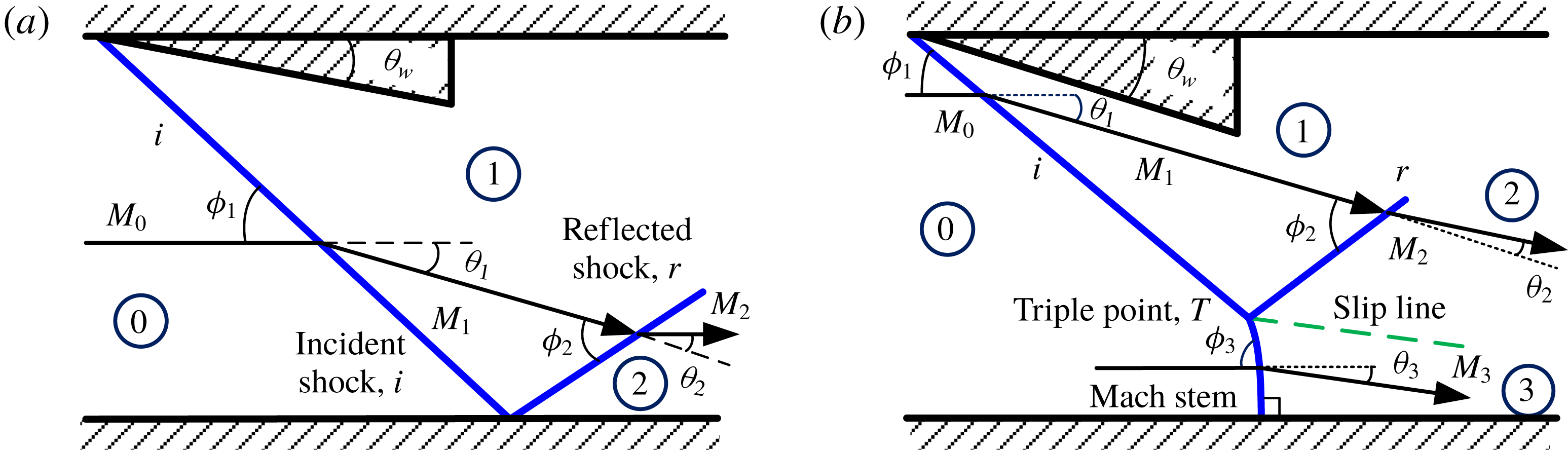
Figure 1. (a) Regular reflection for
 $\unicode[STIX]{x1D703}_{w}<\unicode[STIX]{x1D703}_{w}^{D}(M_{1})<\unicode[STIX]{x1D703}_{w}^{D}(M_{0})$
; (b) Mach reflection for
$\unicode[STIX]{x1D703}_{w}<\unicode[STIX]{x1D703}_{w}^{D}(M_{1})<\unicode[STIX]{x1D703}_{w}^{D}(M_{0})$
; (b) Mach reflection for
 $\unicode[STIX]{x1D703}_{w}^{D}(M_{1})<\unicode[STIX]{x1D703}_{w}<\unicode[STIX]{x1D703}_{w}^{D}(M_{0})$
; where subscript
$\unicode[STIX]{x1D703}_{w}^{D}(M_{1})<\unicode[STIX]{x1D703}_{w}<\unicode[STIX]{x1D703}_{w}^{D}(M_{0})$
; where subscript
 $w$
denotes wedge and superscript
$w$
denotes wedge and superscript
 $D$
denotes detachment criterion.
$D$
denotes detachment criterion.
It was widely accepted that there are two limiting criteria for RR
 $\leftrightarrow$
MR transition in steady flows, namely the von Neumann and the detachment criteria (Von-Neumann Reference Von-Neumann1943, Reference Von-Neumann1945; Henderson & Lozzi Reference Henderson and Lozzi1975; Hornung, Oertel & Sandeman Reference Hornung, Oertel and Sandeman1979). The von Neumann criterion suggests that the RR
$\leftrightarrow$
MR transition in steady flows, namely the von Neumann and the detachment criteria (Von-Neumann Reference Von-Neumann1943, Reference Von-Neumann1945; Henderson & Lozzi Reference Henderson and Lozzi1975; Hornung, Oertel & Sandeman Reference Hornung, Oertel and Sandeman1979). The von Neumann criterion suggests that the RR
 $\leftrightarrow$
MR transition occurs when the static pressures downstream of the reflected shock and the Mach stem match at the triple point. The detachment criterion proposes that RR
$\leftrightarrow$
MR transition occurs when the static pressures downstream of the reflected shock and the Mach stem match at the triple point. The detachment criterion proposes that RR
 $\leftrightarrow$
MR transition happens when the required turning angle for the flow downstream of the incident shock to become parallel to the reflecting surface, exceeds the maximum turning angle possible for that flow Mach number. Above the wedge angle corresponding to the detachment criterion, only MR structure exists, and below the wedge angle corresponding to von Neumann criterion, only RR structure exists.
$\leftrightarrow$
MR transition happens when the required turning angle for the flow downstream of the incident shock to become parallel to the reflecting surface, exceeds the maximum turning angle possible for that flow Mach number. Above the wedge angle corresponding to the detachment criterion, only MR structure exists, and below the wedge angle corresponding to von Neumann criterion, only RR structure exists.
It has been found from all the previous studies that the wedge-angle-variation-induced transition of RR
 $\rightarrow$
MR is abrupt, in the sense that the Mach stem (followed by a region of subsonic flow) appears suddenly. On the other hand, the MR
$\rightarrow$
MR is abrupt, in the sense that the Mach stem (followed by a region of subsonic flow) appears suddenly. On the other hand, the MR
 $\rightarrow$
RR transition is smooth, with the Mach stem height gradually reducing to zero. In other words, the reduction of the Mach stem size to zero presents itself as a corollary to the MR
$\rightarrow$
RR transition is smooth, with the Mach stem height gradually reducing to zero. In other words, the reduction of the Mach stem size to zero presents itself as a corollary to the MR
 $\rightarrow$
RR transition criterion, where the von Neumann condition is satisfied. This led the researchers to the prediction of the height of the Mach stem and the overall MR configuration through geometric considerations, to identify the von Neumann criterion for transition. Efforts towards determining the Mach reflection configurations started with Azevedo (Reference Azevedo1989). He analytically modelled a symmetric MR, as shown in figure 2. In this work, it was assumed that the leading characteristic from the expansion fan (emanating from the trailing edge of the wedge and transmitted by the reflected shock) interacts with the slip line at the sonic throat. This point is shown as
$\rightarrow$
RR transition criterion, where the von Neumann condition is satisfied. This led the researchers to the prediction of the height of the Mach stem and the overall MR configuration through geometric considerations, to identify the von Neumann criterion for transition. Efforts towards determining the Mach reflection configurations started with Azevedo (Reference Azevedo1989). He analytically modelled a symmetric MR, as shown in figure 2. In this work, it was assumed that the leading characteristic from the expansion fan (emanating from the trailing edge of the wedge and transmitted by the reflected shock) interacts with the slip line at the sonic throat. This point is shown as
 $F$
in figure 2. The slip line is taken to be straight until this point.
$F$
in figure 2. The slip line is taken to be straight until this point.
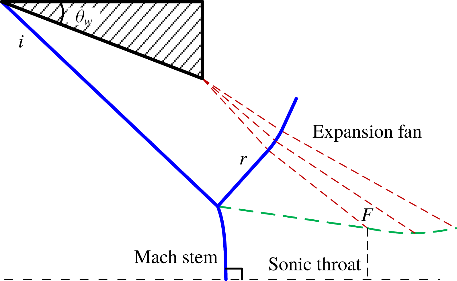
Figure 2. Model for Mach reflection configuration (Azevedo Reference Azevedo1989).
Li & Ben-Dor (Reference Li and Ben-Dor1997) improved this symmetric model by considering additional flow features such as the interaction of the reflected shock with the expansion fan from the trailing edge of the wedge, the entropy layer emanating from this interaction and the reflection of the expansion fan from the slip line. In this model, the slip line starts curving from point
 $F$
onward and becomes parallel to the symmetry plane at a point where the central characteristic of the expansion fan interacts with the slip line and also the sonic throat occurs. They employed a second-order curve to model the curved entities like the Mach stem and segments of the slip line and the reflected shock.
$F$
onward and becomes parallel to the symmetry plane at a point where the central characteristic of the expansion fan interacts with the slip line and also the sonic throat occurs. They employed a second-order curve to model the curved entities like the Mach stem and segments of the slip line and the reflected shock.
Mouton (Reference Mouton2007), Hornung & Mouton (Reference Hornung and Mouton2008) and Mouton & Hornung (Reference Mouton and Hornung2008) suggested another model for symmetric MR, where they considered only the geometrical features of the flow problem and omitted the curvature of the discontinuities (Mach stem, slip line). Further minute details of the MR configuration were considered in more recent models by Gao & Wu (Reference Gao and Wu2010) and Bai & Wu (Reference Bai and Wu2017) to predict the MR configuration. Both these models incorporated the presence of secondary waves emanating from the slip line into the non-uniform supersonic flow and consequent interactions therewith, leading to an inflection in the slip-line curve at point
 $F$
. Bai & Wu (Reference Bai and Wu2017) additionally found a discontinuity in the slope of the slip line.
$F$
. Bai & Wu (Reference Bai and Wu2017) additionally found a discontinuity in the slope of the slip line.
For most practical cases of engineering interest such as supersonic inlet flows, nozzle flows and hypersonic flows, the type of MR is asymmetric rather than symmetric. Two types of configuration are generally observed in asymmetric reflections – overall regular reflection (oRR) and overall Mach reflection (oMR) (Li, Chpoun & Ben-Dor Reference Li, Chpoun and Ben-Dor1999; Ben-Dor Reference Ben-Dor2007). The schematics are given in figure 3. The subscripts
 $u$
and
$u$
and
 $l$
indicate upper and lower regions, respectively.
$l$
indicate upper and lower regions, respectively.

Figure 3. Types of asymmetric reflection: (a) oRR (overall regular reflection); (b) oMR (overall Mach reflection); subscript
 $u$
stands for upper domain and
$u$
stands for upper domain and
 $l$
stands for lower domain.
$l$
stands for lower domain.
Mouton (Reference Mouton2007) defined an equivalence angle to estimate the Mach stem height for asymmetric MR from their symmetric MR model. Recently, Roy & Rajesh (Reference Roy and Rajesh2017) presented an analytical model for asymmetric MR based on the Li & Ben-Dor (Reference Li and Ben-Dor1997) model. Tao et al. (Reference Tao, Liu, Fan, Xiong, Yu and Sun2017) proposed a model for asymmetric MR, based on the Gao & Wu (Reference Gao and Wu2010) symmetric MR model. They claimed that the locations of the triple points are a function of the angles of the two slip lines, which they based on the experimental visualisations of oMR (Tao, Fan & Zhao Reference Tao, Fan and Zhao2015) for some particular conditions. The model takes into consideration the secondary waves on the slip lines as in the case of Gao & Wu (Reference Gao and Wu2010) and the predictions are shown to be in reasonable agreement with previous experimental and numerical data. However, the estimation of Mach stem height for various oMR configurations (figure 4) in the asymmetric wedge-angle–Mach-number domain was never attempted in their work.

Figure 4. Types of overall Mach reflection (based on upper wedge angle): (a) DiMR (direct Mach reflection); (b) StMR (stationary Mach reflection); (c) InMR (inverse Mach reflection).
Figure 4 shows various configurations of oMR in the wedge-angle–Mach-number domain, along with the corresponding shock polars based on the inclinations of the slip line (Li et al. Reference Li, Chpoun and Ben-Dor1999; Ben-Dor Reference Ben-Dor2007). As can be seen from the figure, the InMR configuration is very different from the other oMR configurations. For example, it is not possible to have two InMRs in an oMR as that would result in diverging slip lines and hence render the flow non-physical. InMR is a discrete manifestation only in asymmetric reflection in steady flows.
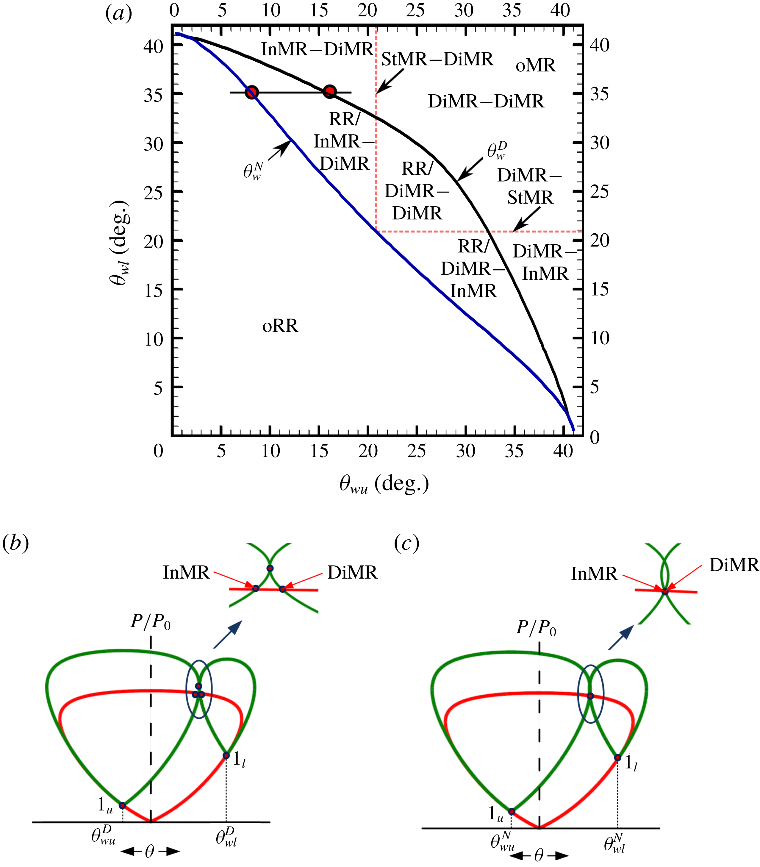
Figure 5. (a) The dual-solution domain in the (
 $\unicode[STIX]{x1D703}_{wu},\unicode[STIX]{x1D703}_{wl}$
)-plane for
$\unicode[STIX]{x1D703}_{wu},\unicode[STIX]{x1D703}_{wl}$
)-plane for
 $M_{0}=4.96$
(Li et al.
Reference Li, Chpoun and Ben-Dor1999); (b,c) shock polars for a set of cases of detachment and von Neumann criteria, respectively.
$M_{0}=4.96$
(Li et al.
Reference Li, Chpoun and Ben-Dor1999); (b,c) shock polars for a set of cases of detachment and von Neumann criteria, respectively.
Various configurations of asymmetric reflection can be better understood with the help of the (
 $\unicode[STIX]{x1D703}_{wu},\unicode[STIX]{x1D703}_{wl}$
)-plane, as given in figure 5(a) for an incoming Mach number
$\unicode[STIX]{x1D703}_{wu},\unicode[STIX]{x1D703}_{wl}$
)-plane, as given in figure 5(a) for an incoming Mach number
 $M_{0}$
of 4.96 (Li et al.
Reference Li, Chpoun and Ben-Dor1999). The figure shows the plots of detachment (
$M_{0}$
of 4.96 (Li et al.
Reference Li, Chpoun and Ben-Dor1999). The figure shows the plots of detachment (
 $\unicode[STIX]{x1D703}_{w}^{D}$
) and von Neumann (
$\unicode[STIX]{x1D703}_{w}^{D}$
) and von Neumann (
 $\unicode[STIX]{x1D703}_{w}^{N}$
) criteria, and the domains of various shock reflections that are theoretically possible for a given set of wedge angles. The region enclosed between the curves demarcates the dual-solution domain, whereby both oRR and oMR solutions are possible. Shock polars for arbitrary wedge angles for the two criteria, which are marked in figure 5(a), are shown in figure 5(b,c).
$\unicode[STIX]{x1D703}_{w}^{N}$
) criteria, and the domains of various shock reflections that are theoretically possible for a given set of wedge angles. The region enclosed between the curves demarcates the dual-solution domain, whereby both oRR and oMR solutions are possible. Shock polars for arbitrary wedge angles for the two criteria, which are marked in figure 5(a), are shown in figure 5(b,c).
Analytical predictions of InMR configurations have not been addressed by previous work on asymmetric MR by Tao et al. (Reference Tao, Liu, Fan, Xiong, Yu and Sun2017), and it is not clear whether their model can correctly predict them. The present work is hence an attempt to develop an analytical model to predict the oMR configurations for all types of steady Mach reflections in asymmetric wedge flows. The present analytical model is based on the Li & Ben-Dor (Reference Li and Ben-Dor1997) model for the simple reason that the model takes into consideration most of the physical phenomena in the shock reflection region. For example, in the Li & Ben-Dor (Reference Li and Ben-Dor1997) model, the triple point solution, the subsonic region, the reflected shock–expansion-fan interaction and the reflection of the expansion fan from the slip line (although there is no appreciable effect (Henderson Reference Henderson1989)) were considered. Moreover, certain flow features such as the Mach stem, reflected shock configuration and slip-line curvatures were approximated using second-order curves. In the following section, the Li & Ben-Dor (Reference Li and Ben-Dor1997) model is discussed, followed by some salient features of the Roy & Rajesh (Reference Roy and Rajesh2017) model, which is extended in the present work. Next, the formulation for the present model is given in detail, and finally, the results obtained by this model are presented and analysed. It is expected that the present work will be a useful addition to the more recent interest in asymmetric Mach reflection configurations in steady flows.
2 Base models
The symmetric MR model by Li & Ben-Dor (Reference Li and Ben-Dor1997) was an improvement over the ones given by Azevedo (Reference Azevedo1989) and Azevedo & Liu (Reference Azevedo and Liu1993). The upper part of figure 6 (highlighted in the dashed box) is the schematic of the symmetric MR configuration employed by Li & Ben-Dor (Reference Li and Ben-Dor1997). The lower part is added for completeness and the whole schematic represents the model proposed by Roy & Rajesh (Reference Roy and Rajesh2017), and serves as the base model for the present work.

Figure 6. Asymmetric MR model (Roy & Rajesh Reference Roy and Rajesh2017); highlighted symmetric MR model (Li & Ben-Dor Reference Li and Ben-Dor1997).
In the Li & Ben-Dor (Reference Li and Ben-Dor1997) model, regions of reflection phenomena are systematically solved for unknown parameters. The governing equations for the flow field are combined and rewritten so as to express the flow properties downstream of a shock as functions of upstream flow Mach number
 $M$
and shock angle
$M$
and shock angle
 $\unicode[STIX]{x1D719}$
. Flow deflections through expansion waves and the shock–expansion-fan interactions are modelled using the Prandtl–Meyer function. The slip line is taken to be a straight line until the location where the leading characteristic from the expansion fan interacts with it. The slip line curves downstream of this point to become parallel to the horizontal line of symmetry at a further downstream location. It is at this location that the sonic throat occurs, where the subsonic pocket of the quasi-one-dimensional flow has the minimum area of cross-section. Downstream of the throat, the flow expands further, with the slip lines diverging as well. Thus the expansion fan from the trailing edge of the wedge determines the size and location of the Mach stem by carrying information of the geometrical features through the subsonic pocket to the Mach stem.
$\unicode[STIX]{x1D719}$
. Flow deflections through expansion waves and the shock–expansion-fan interactions are modelled using the Prandtl–Meyer function. The slip line is taken to be a straight line until the location where the leading characteristic from the expansion fan interacts with it. The slip line curves downstream of this point to become parallel to the horizontal line of symmetry at a further downstream location. It is at this location that the sonic throat occurs, where the subsonic pocket of the quasi-one-dimensional flow has the minimum area of cross-section. Downstream of the throat, the flow expands further, with the slip lines diverging as well. Thus the expansion fan from the trailing edge of the wedge determines the size and location of the Mach stem by carrying information of the geometrical features through the subsonic pocket to the Mach stem.
A salient feature of the Li & Ben-Dor (Reference Li and Ben-Dor1997) model is that the shape of the Mach stem is assumed to be slightly curved, and modelled using a second-order curve as a function of the boundary conditions (coordinates and slope at its ends), under a first-order approximation assuming minimal change in slope. Other similar shapes, such as the curved portion of the slip line and the characteristic lines of the expansion fan in the entropy layer region, are also modelled using this relation. The equation of the curve (Li & Ben-Dor Reference Li and Ben-Dor1997) is as follows:
 $$\begin{eqnarray}\displaystyle & & \displaystyle J(x,y,x_{1},y_{1},x_{2},y_{2},\unicode[STIX]{x1D6FF}_{1},\unicode[STIX]{x1D6FF}_{2})=[(y-y_{1})\sin \unicode[STIX]{x1D6FF}_{1}+(x-x_{1})\cos \unicode[STIX]{x1D6FF}_{1}]^{2}\tan (\unicode[STIX]{x1D6FF}_{2}-\unicode[STIX]{x1D6FF}_{1})\nonumber\\ \displaystyle & & \displaystyle \quad +\,2[(x_{2}-x_{1})\cos \unicode[STIX]{x1D6FF}_{1}+(y_{2}-y_{1})\sin \unicode[STIX]{x1D6FF}_{1}][(x-x_{1})\sin \unicode[STIX]{x1D6FF}_{1}-(y-y_{1})\cos \unicode[STIX]{x1D6FF}_{1}]=0\qquad\end{eqnarray}$$
and the coordinates of the end points
 $[(x_{1},y_{1}),(x_{2},y_{2})]$
satisfy the relation:
$[(x_{1},y_{1}),(x_{2},y_{2})]$
satisfy the relation:
 $$\begin{eqnarray}y_{2}-y_{1}=\tan \unicode[STIX]{x1D6EC}[\unicode[STIX]{x1D6FF}_{1},\unicode[STIX]{x1D6FF}_{2}](x_{2}-x_{1}),\end{eqnarray}$$
where
 $(\unicode[STIX]{x1D6FF}_{1},\unicode[STIX]{x1D6FF}_{2})$
are the slopes (with
$(\unicode[STIX]{x1D6FF}_{1},\unicode[STIX]{x1D6FF}_{2})$
are the slopes (with
 $x$
-axis) at the ends, and
$x$
-axis) at the ends, and
 $\unicode[STIX]{x1D6EC}$
is given by:
$\unicode[STIX]{x1D6EC}$
is given by:
 $$\begin{eqnarray}\unicode[STIX]{x1D6EC}(\unicode[STIX]{x1D6FF}_{1},\unicode[STIX]{x1D6FF}_{2})=\arctan \left[\frac{2\tan \unicode[STIX]{x1D6FF}_{1}+\tan (\unicode[STIX]{x1D6FF}_{2}-\unicode[STIX]{x1D6FF}_{1})}{2-\tan \unicode[STIX]{x1D6FF}_{1}\tan (\unicode[STIX]{x1D6FF}_{2}-\unicode[STIX]{x1D6FF}_{1})}\right].\end{eqnarray}$$
Roy & Rajesh (Reference Roy and Rajesh2017) proposed the model for asymmetric MR as a combination of upper and lower domains of symmetric MR, as shown in figure 6. Here, the axis of symmetry (for symmetric MR) is taken as the common horizontal
 $x$
-axis for both the upper and lower domains. By inverting the vertical axis of the coordinate system in the lower domain (
$x$
-axis for both the upper and lower domains. By inverting the vertical axis of the coordinate system in the lower domain (
 $y_{u}$
to
$y_{u}$
to
 $y_{l}$
), all the conventions used for the geometrical parameters in the upper domain are retained.
$y_{l}$
), all the conventions used for the geometrical parameters in the upper domain are retained.

Figure 7. Conditions for closing the equations in Roy & Rajesh (Reference Roy and Rajesh2017) model: (a) choking at the same abscissa; (b) sonic (choking) contour along the Mach stem profile; (c) profile continuity of the Mach stem.
The flow domains around the triple point, and the region of interaction of the expansion fan with the reflected shock, for both the upper and lower domains, were solved independently. The geometrical relations for the upper and lower domains were grouped together to be solved simultaneously, which yielded a set of 23 equations with 24 unknowns. Various possible closing equations were proposed in Roy & Rajesh (Reference Roy and Rajesh2017) and the results for the oMR configurations were compared. Figure 7 gives schematic representations of the closing equations proposed. In figure 7(a), the flow in the subsonic pocket is assumed to choke at the same horizontal location, giving a straight vertical line profile to the sonic contour. In figure 7(b), the sonic contour is assumed to follow the Mach stem profile by following the exact curvature of the stem. The third approach, which is more fundamental, is shown schematically in figure 7(c). Here, it is imposed that the Mach stem has a continuous profile across the upper and lower domains, with the slopes being equal (and perpendicular) at the point of confluence on the axis. This condition for the closing equation was previously concluded to give the best results (Roy & Rajesh Reference Roy and Rajesh2017), and has been subsequently used in the present study as well.
Figure 8. Position of common
 $x$
-axis in Roy & Rajesh (Reference Roy and Rajesh2017) model: (a) DiMR–DiMR; (b) StMR–DiMR; (c) InMR–DiMR (hypothetical).
$x$
-axis in Roy & Rajesh (Reference Roy and Rajesh2017) model: (a) DiMR–DiMR; (b) StMR–DiMR; (c) InMR–DiMR (hypothetical).
In the Roy & Rajesh (Reference Roy and Rajesh2017) model, the Mach stem is perpendicular to a common
 $x$
-axis. It is argued that there is at least one streamline in the uniform flow upstream that passes through the Mach stem without deviation, and this streamline essentially forms the
$x$
-axis. It is argued that there is at least one streamline in the uniform flow upstream that passes through the Mach stem without deviation, and this streamline essentially forms the
 $x$
-axis. The vertical location of the
$x$
-axis. The vertical location of the
 $x$
-axis is variable and depends on the particular case of oMR configuration, as shown in figure 8. In case of DiMR–DiMR, the axis passes through the Mach stem at some intermediate position between the triple points. The axis keeps shifting to any of the triple points for decreasing wedge angle of the corresponding side. The limiting case occurs for StMR–DiMR in which the axis passes through one of the triple points and is also perpendicular to the Mach stem at that point, and the contribution to the Mach stem height is made entirely by the domain on one side of the axis. Although this approach works well for the DiMR–DiMR or DiMR–StMR case, it cannot give the solution for the condition when one of the reflections is an InMR, as shown in figure 8(c). Here, the axis becomes perpendicular to the Mach stem at a hypothetically extrapolated location. In this case, the axis cannot be taken as a symmetry plane for any of the symmetric MR halves. This limitation, in particular, has been addressed and resolved in the present work.
$x$
-axis is variable and depends on the particular case of oMR configuration, as shown in figure 8. In case of DiMR–DiMR, the axis passes through the Mach stem at some intermediate position between the triple points. The axis keeps shifting to any of the triple points for decreasing wedge angle of the corresponding side. The limiting case occurs for StMR–DiMR in which the axis passes through one of the triple points and is also perpendicular to the Mach stem at that point, and the contribution to the Mach stem height is made entirely by the domain on one side of the axis. Although this approach works well for the DiMR–DiMR or DiMR–StMR case, it cannot give the solution for the condition when one of the reflections is an InMR, as shown in figure 8(c). Here, the axis becomes perpendicular to the Mach stem at a hypothetically extrapolated location. In this case, the axis cannot be taken as a symmetry plane for any of the symmetric MR halves. This limitation, in particular, has been addressed and resolved in the present work.
3 Formulation of asymmetric MR configuration model
This section contains the detailed formulation for the present asymmetric MR model. The algorithm has been coded in Python, and particularly makes use of the scipy module.

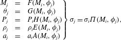
Figure 9. Schematic of asymmetric Mach reflection model.
 $H_{t}$
is the total height between the wedges. Subscripts
$H_{t}$
is the total height between the wedges. Subscripts
 $u$
and
$u$
and
 $l$
depict the upper and lower regions, respectively, with respect to the
$l$
depict the upper and lower regions, respectively, with respect to the
 $x$
axis upstream of the Mach stem and the inclined axis
$x$
axis upstream of the Mach stem and the inclined axis
 $x_{i}$
downstream of the Mach stem.
$x_{i}$
downstream of the Mach stem.
 $H$
is the height of the leading edge of the wedge, measured from the common horizontal
$H$
is the height of the leading edge of the wedge, measured from the common horizontal
 $x$
-axis. The wedge slant length is given as
$x$
-axis. The wedge slant length is given as
 $w$
.
$w$
.
 $H_{m}$
is the Mach stem height, i.e. distance of the triple point from the
$H_{m}$
is the Mach stem height, i.e. distance of the triple point from the
 $x$
-axis.
$x$
-axis.
 $H_{s}$
is the height of the sonic throat, measured from axis
$H_{s}$
is the height of the sonic throat, measured from axis
 $x_{i}$
.
$x_{i}$
.
 $i$
is the incident shock,
$i$
is the incident shock,
 $r$
is the reflected shock,
$r$
is the reflected shock,
 $r^{\prime }$
is the reflected shock after interaction with the expansion fan,
$r^{\prime }$
is the reflected shock after interaction with the expansion fan,
 $s$
is the slip line.
$s$
is the slip line.
 $L$
is the horizontal gap between the wedges.
$L$
is the horizontal gap between the wedges.
A schematic of the present model is given in figure 9. An inverse MR configuration is given in particular to emphasise the detailed formulation of the present model for InMR cases, while all the other oMR configurations are also analysed. On comparing the present model with the earlier model (Roy & Rajesh Reference Roy and Rajesh2017) given in figure 6, it is to be noted that the subsonic convergent–divergent pocket downstream of the Mach stem, is assumed to be oriented along an inclined axis
 $x_{i}$
, rather than parallel to and in continuation with the common horizontal
$x_{i}$
, rather than parallel to and in continuation with the common horizontal
 $x$
-axis, where the angle of inclination (
$x$
-axis, where the angle of inclination (
 $\unicode[STIX]{x1D703}_{4}$
) is the average of the angles at which the streamlines are deflected by the Mach stem at the two triple points. It is argued that at least one streamline from the upstream uniform flow is deflected at this average angle (
$\unicode[STIX]{x1D703}_{4}$
) is the average of the angles at which the streamlines are deflected by the Mach stem at the two triple points. It is argued that at least one streamline from the upstream uniform flow is deflected at this average angle (
 $\unicode[STIX]{x1D703}_{4}$
) by the Mach stem, at an intermediate location between the two triple points. This incoming streamline before the Mach stem, and its extension beyond the point of deflection, forms the common horizontal
$\unicode[STIX]{x1D703}_{4}$
) by the Mach stem, at an intermediate location between the two triple points. This incoming streamline before the Mach stem, and its extension beyond the point of deflection, forms the common horizontal
 $x$
-axis. The direction of the deflected streamline behind the Mach stem is taken to be the inclined axis
$x$
-axis. The direction of the deflected streamline behind the Mach stem is taken to be the inclined axis
 $x_{i}$
. Although the subsonic flow behind the Mach stem is known to be non-uniform, the axis
$x_{i}$
. Although the subsonic flow behind the Mach stem is known to be non-uniform, the axis
 $x_{i}$
indicates the mean orientation of the flow, which is assumed to be quasi-one-dimensional for the present study.
$x_{i}$
indicates the mean orientation of the flow, which is assumed to be quasi-one-dimensional for the present study.
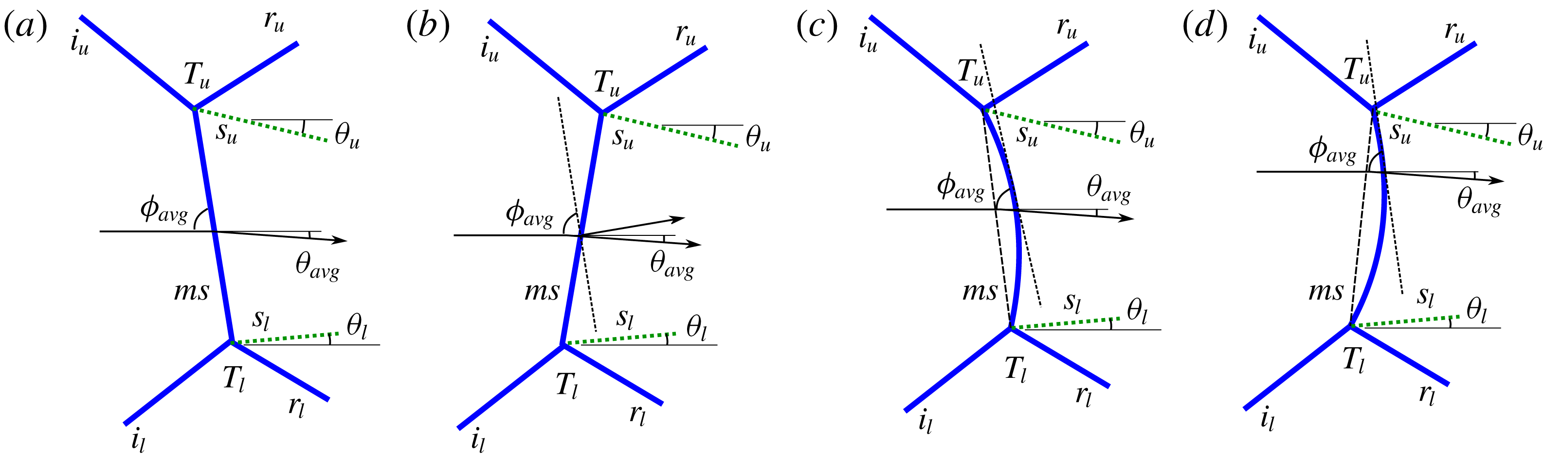
Figure 10. Based on theory given by Tao et al. (Reference Tao, Liu, Fan, Xiong, Yu and Sun2017), (a)
 $x_{Tu}<x_{Tl}$
, (b)
$x_{Tu}<x_{Tl}$
, (b)
 $x_{Tu}>x_{Tl}$
; based on present model, (c)
$x_{Tu}>x_{Tl}$
; based on present model, (c)
 $x_{Tu}<x_{Tl}$
, (d)
$x_{Tu}<x_{Tl}$
, (d)
 $x_{Tu}>x_{Tl}$
.
$x_{Tu}>x_{Tl}$
.
A somewhat seemingly similar approach can be seen in Tao et al. (Reference Tao, Liu, Fan, Xiong, Yu and Sun2017). Figure 10 gives a comparison of their approach and that of the present model. Tao et al. (Reference Tao, Liu, Fan, Xiong, Yu and Sun2017) employed an average deflection angle
 $\unicode[STIX]{x1D703}_{avg}$
, given by the mean of the slip-line angles with respect to the incoming flow upstream of the Mach stem
$\unicode[STIX]{x1D703}_{avg}$
, given by the mean of the slip-line angles with respect to the incoming flow upstream of the Mach stem
 $ms$
near the two triple points
$ms$
near the two triple points
 $T_{u}$
and
$T_{u}$
and
 $T_{l}$
. This is used to calculate the relative locations of the triple points based on the orientation of a straight oblique shock obtained from this average deflection angle. This is shown in figure 10(a). It is our understanding that the von Neumann three-shock theory gives only the angles and flow properties near each triple point for given wedge angles, whereas the locations of the triple points are influenced by the geometry and the Mach number of the incoming flow. The geometry comprises of the wedge angles as well as the relative positioning of the wedges. However, in Tao et al.’s (Reference Tao, Liu, Fan, Xiong, Yu and Sun2017) model, the
$T_{l}$
. This is used to calculate the relative locations of the triple points based on the orientation of a straight oblique shock obtained from this average deflection angle. This is shown in figure 10(a). It is our understanding that the von Neumann three-shock theory gives only the angles and flow properties near each triple point for given wedge angles, whereas the locations of the triple points are influenced by the geometry and the Mach number of the incoming flow. The geometry comprises of the wedge angles as well as the relative positioning of the wedges. However, in Tao et al.’s (Reference Tao, Liu, Fan, Xiong, Yu and Sun2017) model, the
 $\unicode[STIX]{x1D703}_{avg}$
fixes the triple point locations. This is elucidated in figure 10(b), where the average flow deflection, which is downward, requires a straight right running oblique shock (
$\unicode[STIX]{x1D703}_{avg}$
fixes the triple point locations. This is elucidated in figure 10(b), where the average flow deflection, which is downward, requires a straight right running oblique shock (
 $x_{Tu}<x_{Tl}$
as in figure 10
a) and is shown by the dotted line. However, by virtue of the geometry (location of the wedges), the triple points may be located in such a way that
$x_{Tu}<x_{Tl}$
as in figure 10
a) and is shown by the dotted line. However, by virtue of the geometry (location of the wedges), the triple points may be located in such a way that
 $x_{Tu}>x_{Tl}$
, which forms a left running shock. In the present model, this ambiguity is removed by considering the curvature of the Mach stem
$x_{Tu}>x_{Tl}$
, which forms a left running shock. In the present model, this ambiguity is removed by considering the curvature of the Mach stem
 $ms$
which is modelled as a second-order curve using (2.1) to (2.3). Here, the average flow deflection
$ms$
which is modelled as a second-order curve using (2.1) to (2.3). Here, the average flow deflection
 $\unicode[STIX]{x1D703}_{avg}$
is used to estimate a location on the curved Mach stem where the inclination would be the same as that of an oblique shock at a shock angle
$\unicode[STIX]{x1D703}_{avg}$
is used to estimate a location on the curved Mach stem where the inclination would be the same as that of an oblique shock at a shock angle
 $\unicode[STIX]{x1D719}_{avg}$
. This accommodates both the cases as shown in figure 10(c,d). The only difference is that vertical location of
$\unicode[STIX]{x1D719}_{avg}$
. This accommodates both the cases as shown in figure 10(c,d). The only difference is that vertical location of
 $x$
-axis is shifted along the Mach stem.
$x$
-axis is shifted along the Mach stem.
The governing equations used for this model are based on the assumptions as stated in Li & Ben-Dor (Reference Li and Ben-Dor1997). A stable MR configuration exists in the absence of far-field downstream disturbances. The fluid in consideration is ideal and hence its dynamic viscosity and thermal conductivity are zero. The gas is perfect, with a constant heat capacity ratio
 $\unicode[STIX]{x1D6FE}$
. The flow in region 2 (see figure 9) is supersonic. The slip lines form a two-dimensional convergent–divergent nozzle, whereby the subsonic flow behind the Mach stem accelerates to become sonic at the throat. Any secondary waves reflected from the slip lines (Gao & Wu Reference Gao and Wu2010; Bai & Wu Reference Bai and Wu2017) have been ignored here, with the understanding that their contribution is not significant in comparison to the primary waves in the overall shock reflection configuration (Ben-Dor Reference Ben-Dor2007, § 2.3.4).
$\unicode[STIX]{x1D6FE}$
. The flow in region 2 (see figure 9) is supersonic. The slip lines form a two-dimensional convergent–divergent nozzle, whereby the subsonic flow behind the Mach stem accelerates to become sonic at the throat. Any secondary waves reflected from the slip lines (Gao & Wu Reference Gao and Wu2010; Bai & Wu Reference Bai and Wu2017) have been ignored here, with the understanding that their contribution is not significant in comparison to the primary waves in the overall shock reflection configuration (Ben-Dor Reference Ben-Dor2007, § 2.3.4).
Geometrical inputs required for the model include the total height
 $H_{t}$
between the leading edges of the wedges, the slant lengths
$H_{t}$
between the leading edges of the wedges, the slant lengths
 $w_{u}$
and
$w_{u}$
and
 $w_{l}$
of the wedges and the respective deflection angles
$w_{l}$
of the wedges and the respective deflection angles
 $\unicode[STIX]{x1D703}_{wu}$
and
$\unicode[STIX]{x1D703}_{wu}$
and
 $\unicode[STIX]{x1D703}_{wl}$
. The Mach number of the incoming flow is required, along with flow properties such as pressure and temperature from which the thermodynamic state variables are to be calculated.
$\unicode[STIX]{x1D703}_{wl}$
. The Mach number of the incoming flow is required, along with flow properties such as pressure and temperature from which the thermodynamic state variables are to be calculated.
The region 0 has uniform flow field before the shock structure, and is common to both the upper and lower domains. Region 1 has uniform supersonic flow conditions after being deflected by the incident shock
 $i$
. It extends till the region bound by the leading characteristic of the expansion fan emanating from the trailing edge of the wedge. Region
$i$
. It extends till the region bound by the leading characteristic of the expansion fan emanating from the trailing edge of the wedge. Region
 $2$
has flow conditions after the flow field passes through the reflected shock
$2$
has flow conditions after the flow field passes through the reflected shock
 $r$
. It also extends until and is bound by the leading characteristic of the expansion fan from the trailing edge of the wedge. Region
$r$
. It also extends until and is bound by the leading characteristic of the expansion fan from the trailing edge of the wedge. Region
 $3$
is the area past the Mach stem
$3$
is the area past the Mach stem
 $ms$
and below the slip line
$ms$
and below the slip line
 $s$
and in close vicinity of the triple point
$s$
and in close vicinity of the triple point
 $T$
. Region
$T$
. Region
 $4$
lies downstream of the Mach stem, in the vicinity of the
$4$
lies downstream of the Mach stem, in the vicinity of the
 $x$
-axis, and demarcates the interface of the upper and lower domains at the Mach stem. Subscripts
$x$
-axis, and demarcates the interface of the upper and lower domains at the Mach stem. Subscripts
 $u$
and
$u$
and
 $l$
depict the upper and lower domains, respectively. The equations in the following subsections apply to each of the domains, and have been written without the respective subscripts, unless specifically required.
$l$
depict the upper and lower domains, respectively. The equations in the following subsections apply to each of the domains, and have been written without the respective subscripts, unless specifically required.
3.1 Triple point
First, we consider the region near the triple points, given in figure 11. The classic von Neumann three-shock theory is applied individually to each triple point, which is the point of confluence of four discontinuities: incident shock
 $i$
, reflected shock
$i$
, reflected shock
 $r$
, Mach stem
$r$
, Mach stem
 $ms$
and slip line
$ms$
and slip line
 $s$
.
$s$
.
The sign conventions for the angles are as shown in figure 11. Since the vertical axis is inverted for the lower domain, the sign conventions are also reversed. For the general case of DiMR given in figure 11(c), the flow deflection angle
 $\unicode[STIX]{x1D703}_{3l}$
is taken to be positive for any deviation of the streamline towards the
$\unicode[STIX]{x1D703}_{3l}$
is taken to be positive for any deviation of the streamline towards the
 $x$
-axis by a left running shock wave, as in the segment of the Mach stem in this domain. The shock angle
$x$
-axis by a left running shock wave, as in the segment of the Mach stem in this domain. The shock angle
 $\unicode[STIX]{x1D719}_{3l}$
is acute. On the other hand, the upper domain given in figure 11(b) has an InMR. Following the sign conventions, the flow deflection angle
$\unicode[STIX]{x1D719}_{3l}$
is acute. On the other hand, the upper domain given in figure 11(b) has an InMR. Following the sign conventions, the flow deflection angle
 $\unicode[STIX]{x1D703}_{3u}$
(depicted as
$\unicode[STIX]{x1D703}_{3u}$
(depicted as
 $-\unicode[STIX]{x1D703}_{3u}$
for clarity) is negative. The segment of the Mach stem in this domain is a left running shock wave (instead of a right running wave if it were a DiMR). Hence, in accordance with the mathematics, the shock angle
$-\unicode[STIX]{x1D703}_{3u}$
for clarity) is negative. The segment of the Mach stem in this domain is a left running shock wave (instead of a right running wave if it were a DiMR). Hence, in accordance with the mathematics, the shock angle
 $\unicode[STIX]{x1D719}_{3u}$
is taken as obtuse. (The angle would be acute for DiMR and
$\unicode[STIX]{x1D719}_{3u}$
is taken as obtuse. (The angle would be acute for DiMR and
 $90^{\circ }$
for StMR.)
$90^{\circ }$
for StMR.)
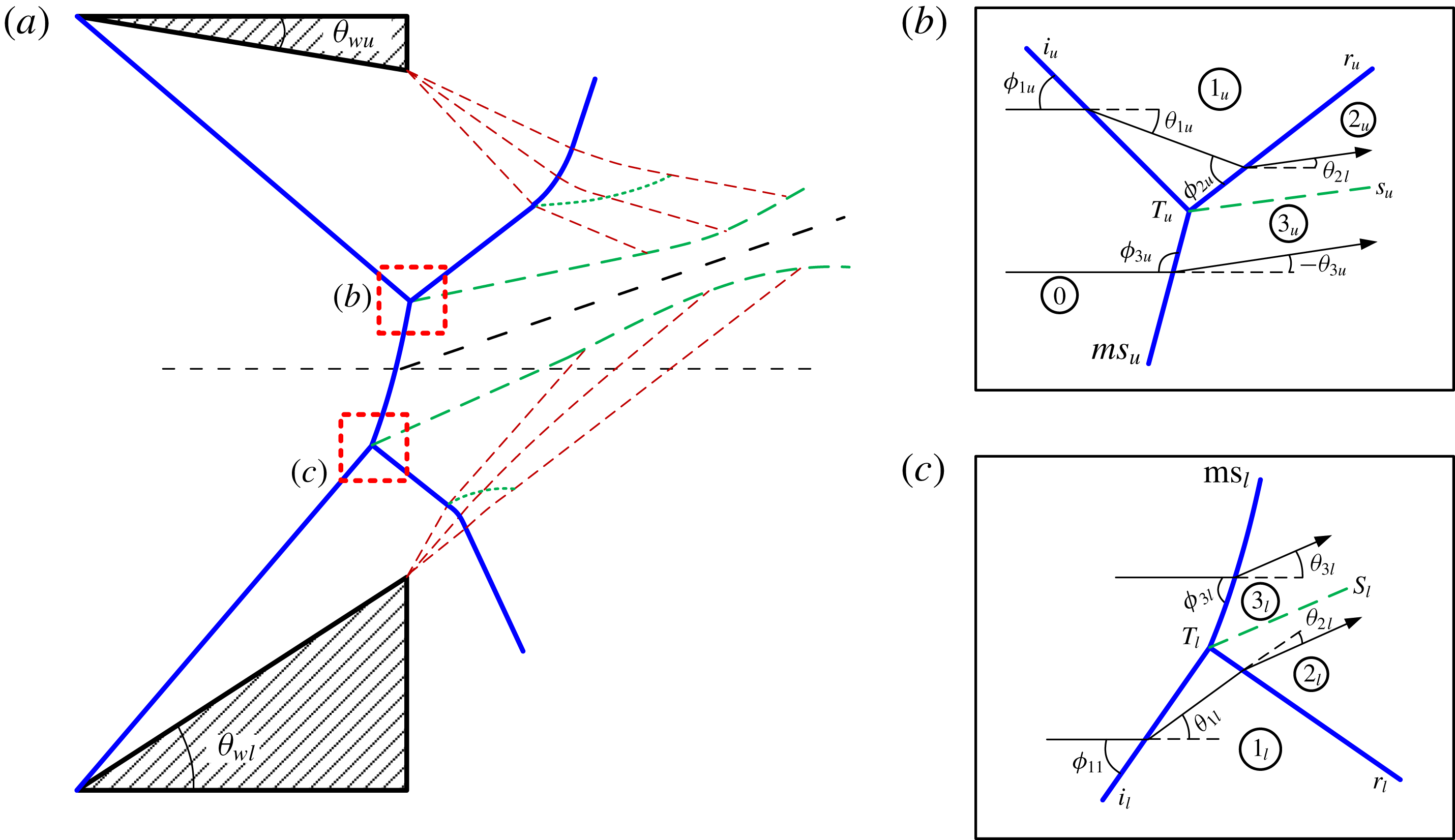
Figure 11. (a) Schematic of asymmetric MR; insets (b) upper triple point region, and (c) lower triple point region.
The following equations are used to relate the downstream properties (
 $j$
) to the upstream ones (
$j$
) to the upstream ones (
 $i$
) across an oblique shock. The details of these relations, which are derived from the conservation equations, can be found in Li & Ben-Dor (Reference Li and Ben-Dor1997) and Ben-Dor (Reference Ben-Dor2007). Here the flow properties are – Mach number
$i$
) across an oblique shock. The details of these relations, which are derived from the conservation equations, can be found in Li & Ben-Dor (Reference Li and Ben-Dor1997) and Ben-Dor (Reference Ben-Dor2007). Here the flow properties are – Mach number
 $M$
, shock angle
$M$
, shock angle
 $\unicode[STIX]{x1D719}$
, pressure
$\unicode[STIX]{x1D719}$
, pressure
 $P$
, flow deflection angle
$P$
, flow deflection angle
 $\unicode[STIX]{x1D703}$
, density
$\unicode[STIX]{x1D703}$
, density
 $\unicode[STIX]{x1D70C}$
and local acoustic speed
$\unicode[STIX]{x1D70C}$
and local acoustic speed
 $a$
.
$a$
.
 $$\begin{eqnarray}\left.\begin{array}{@{}rcl@{}}\displaystyle M_{j} & = & F(M_{i},\unicode[STIX]{x1D719}_{j})\\ \unicode[STIX]{x1D703}_{j} & = & G(M_{i},\unicode[STIX]{x1D719}_{j})\\ P_{j} & = & P_{i}H(M_{i},\unicode[STIX]{x1D719}_{j})\\ \unicode[STIX]{x1D70C}_{j} & = & \unicode[STIX]{x1D70C}_{i}E(M_{i},\unicode[STIX]{x1D719}_{j})\\ a_{j} & = & a_{i}A(M_{i},\unicode[STIX]{x1D719}_{j})\end{array}\right\}\unicode[STIX]{x1D70E}_{j}=\unicode[STIX]{x1D70E}_{i}\unicode[STIX]{x1D6F1}(M_{i},\unicode[STIX]{x1D719}_{j}),\end{eqnarray}$$
where, the functions are given as,
 $$\begin{eqnarray}\displaystyle & \displaystyle F(M,\unicode[STIX]{x1D719})=\left[\frac{1+(\unicode[STIX]{x1D6FE}-1)M^{2}\sin ^{2}\unicode[STIX]{x1D719}+\left[\displaystyle \frac{(\unicode[STIX]{x1D6FE}+1)^{2}}{4}-\unicode[STIX]{x1D6FE}\sin ^{2}\unicode[STIX]{x1D719}\right]M^{4}\sin ^{2}\unicode[STIX]{x1D719}}{\left[\unicode[STIX]{x1D6FE}M^{2}\sin ^{2}\unicode[STIX]{x1D719}-\displaystyle \frac{\unicode[STIX]{x1D6FE}-1}{2}\right]\left[\displaystyle \frac{\unicode[STIX]{x1D6FE}-1}{2}M^{2}\sin ^{2}\unicode[STIX]{x1D719}+1\right]}\right]^{1/2} & \displaystyle\end{eqnarray}$$
 $$\begin{eqnarray}\displaystyle & \displaystyle G(M,\unicode[STIX]{x1D719})=\arctan \left[2\cot \unicode[STIX]{x1D719}\frac{M^{2}\sin ^{2}\unicode[STIX]{x1D719}-1}{M^{2}(\unicode[STIX]{x1D6FE}+\cos 2\unicode[STIX]{x1D719})+2}\right] & \displaystyle\end{eqnarray}$$
 $$\begin{eqnarray}\displaystyle & \displaystyle H(M,\unicode[STIX]{x1D719})=\frac{2}{\unicode[STIX]{x1D6FE}+1}\left[\unicode[STIX]{x1D6FE}M^{2}\sin ^{2}\unicode[STIX]{x1D719}-\frac{\unicode[STIX]{x1D6FE}-1}{2}\right] & \displaystyle\end{eqnarray}$$
 $$\begin{eqnarray}\displaystyle & \displaystyle E(M,\unicode[STIX]{x1D719})=\frac{(\unicode[STIX]{x1D6FE}+1)M^{2}\sin ^{2}\unicode[STIX]{x1D719}}{(\unicode[STIX]{x1D6FE}-1)M^{2}\sin ^{2}\unicode[STIX]{x1D719}+2} & \displaystyle\end{eqnarray}$$
 $$\begin{eqnarray}\displaystyle & \displaystyle A(M,\unicode[STIX]{x1D719})=\frac{[(\unicode[STIX]{x1D6FE}-1)M^{2}\sin ^{2}\unicode[STIX]{x1D719}+2]^{1/2}[2\unicode[STIX]{x1D6FE}M^{2}\sin ^{2}\unicode[STIX]{x1D719}-(\unicode[STIX]{x1D6FE}-1)]^{1/2}}{(\unicode[STIX]{x1D6FE}+1)M\sin \unicode[STIX]{x1D719}}. & \displaystyle\end{eqnarray}$$
Across the incident shock
 $i$
, we have:
$i$
, we have:
 $$\begin{eqnarray}\unicode[STIX]{x1D70E}_{1}=\unicode[STIX]{x1D70E}_{0}\unicode[STIX]{x1D6F1}(M_{0},\unicode[STIX]{x1D719}_{1}).\end{eqnarray}$$
Then, across the reflected shock
 $r$
, we have:
$r$
, we have:
 $$\begin{eqnarray}\unicode[STIX]{x1D70E}_{2}=\unicode[STIX]{x1D70E}_{1}\unicode[STIX]{x1D6F1}(M_{1},\unicode[STIX]{x1D719}_{2}).\end{eqnarray}$$
And, across the Mach stem
 $ms$
, we have:
$ms$
, we have:
 $$\begin{eqnarray}\unicode[STIX]{x1D70E}_{3}=\unicode[STIX]{x1D70E}_{0}\unicode[STIX]{x1D6F1}(M_{0},\unicode[STIX]{x1D719}_{3}).\end{eqnarray}$$
It is to be noted here that weak shock solutions for (3.3) and (3.4), and strong shock solutions for (3.5), are to be considered.
Finally, we have the following boundary conditions:
 $$\begin{eqnarray}\displaystyle \unicode[STIX]{x1D703}_{1}=\unicode[STIX]{x1D703}_{w},\quad P_{3}=P_{2}\quad \text{and}\quad \unicode[STIX]{x1D703}_{3}=\unicode[STIX]{x1D703}_{1}-\unicode[STIX]{x1D703}_{2}. & & \displaystyle\end{eqnarray}$$
The above set of 18 equations are solved for the 18 unknowns:
 $M_{1}$
,
$M_{1}$
,
 $M_{2}$
,
$M_{2}$
,
 $M_{3}$
,
$M_{3}$
,
 $P_{1}$
,
$P_{1}$
,
 $P_{2}$
,
$P_{2}$
,
 $P_{3}$
,
$P_{3}$
,
 $\unicode[STIX]{x1D719}_{1}$
,
$\unicode[STIX]{x1D719}_{1}$
,
 $\unicode[STIX]{x1D719}_{2}$
,
$\unicode[STIX]{x1D719}_{2}$
,
 $\unicode[STIX]{x1D719}_{3}$
,
$\unicode[STIX]{x1D719}_{3}$
,
 $\unicode[STIX]{x1D703}_{1}$
,
$\unicode[STIX]{x1D703}_{1}$
,
 $\unicode[STIX]{x1D703}_{2}$
,
$\unicode[STIX]{x1D703}_{2}$
,
 $\unicode[STIX]{x1D703}_{3}$
,
$\unicode[STIX]{x1D703}_{3}$
,
 $\unicode[STIX]{x1D70C}_{1}$
,
$\unicode[STIX]{x1D70C}_{1}$
,
 $\unicode[STIX]{x1D70C}_{2}$
,
$\unicode[STIX]{x1D70C}_{2}$
,
 $\unicode[STIX]{x1D70C}_{3}$
,
$\unicode[STIX]{x1D70C}_{3}$
,
 $a_{1}$
,
$a_{1}$
,
 $a_{2}$
and
$a_{2}$
and
 $a_{3}$
.
$a_{3}$
.
For the particular configuration of MR shown in figures 9 and 11, the solution would yield a negative value of
 $\unicode[STIX]{x1D703}_{3u}$
in the upper domain. This negative value is in accordance with the sign convention and is to be retained as such.
$\unicode[STIX]{x1D703}_{3u}$
in the upper domain. This negative value is in accordance with the sign convention and is to be retained as such.
While solving the region around the triple points in the upper and lower domains, it is not particularly required to include equations for
 $\unicode[STIX]{x1D70C}$
and
$\unicode[STIX]{x1D70C}$
and
 $a$
in the set to be solved simultaneously; the set of equations would otherwise contain 12 equations and 12 unknowns, and could be solved nevertheless. However, these quantities are being solved for, as they are required in the upcoming subsection.
$a$
in the set to be solved simultaneously; the set of equations would otherwise contain 12 equations and 12 unknowns, and could be solved nevertheless. However, these quantities are being solved for, as they are required in the upcoming subsection.
As evident from the formulation above, each region around a triple point can be solved for, independent of other geometric and/or physical constraints. Consequently, the angle of deflection of the slip line from the
 $x$
-axis (and hence the classification among DiMR, StMR or InMR) at either of the triple points is independent of the other.
$x$
-axis (and hence the classification among DiMR, StMR or InMR) at either of the triple points is independent of the other.
3.2 Subsonic pocket downstream of the Mach stem
3.2.1 Average deflection at the Mach stem
As stated earlier, the inclination of the axis
 $x_{i}$
is based on an average deflection of the flow by the Mach stem, given as:
$x_{i}$
is based on an average deflection of the flow by the Mach stem, given as:
 $$\begin{eqnarray}\unicode[STIX]{x1D703}_{4}=\unicode[STIX]{x1D703}_{avg}=\frac{(-\unicode[STIX]{x1D703}_{3u})+\unicode[STIX]{x1D703}_{3l}}{2}.\end{eqnarray}$$
The opposite signs of
 $\unicode[STIX]{x1D703}$
for regions
$\unicode[STIX]{x1D703}$
for regions
 $3_{u}$
and
$3_{u}$
and
 $3_{l}$
are evoked so as to comply with the flipped
$3_{l}$
are evoked so as to comply with the flipped
 $y$
-axes (and sign conventions) of the upper and lower domains. In this subsection, a positive sign is given to angles measured anticlockwise, as for
$y$
-axes (and sign conventions) of the upper and lower domains. In this subsection, a positive sign is given to angles measured anticlockwise, as for
 $\unicode[STIX]{x1D703}_{4}$
and
$\unicode[STIX]{x1D703}_{4}$
and
 $\unicode[STIX]{x1D703}_{3l}$
.
$\unicode[STIX]{x1D703}_{3l}$
.
With the Mach stem being modelled as a monotonic second-order curve with continuous slope and no inflection point (using (2.1)–(2.3)), there exists exactly a single location on the Mach stem at which the incoming streamline is deflected by
 $\unicode[STIX]{x1D703}_{4}$
. This location is named
$\unicode[STIX]{x1D703}_{4}$
. This location is named
 $G$
, as given in figure 9. The
$G$
, as given in figure 9. The
 $x$
-axis passes through this point on the Mach stem, while its location on the Mach stem itself (given by
$x$
-axis passes through this point on the Mach stem, while its location on the Mach stem itself (given by
 $H_{u}$
and
$H_{u}$
and
 $H_{l}$
) is a variable as of yet.
$H_{l}$
) is a variable as of yet.
To keep in line with the sign conventions of each domain, we henceforward redefine
 $\unicode[STIX]{x1D703}_{4}$
as:
$\unicode[STIX]{x1D703}_{4}$
as:
 $$\begin{eqnarray}\displaystyle \unicode[STIX]{x1D703}_{4^{\prime }u}=-\unicode[STIX]{x1D703}_{4}\quad \text{and}\quad \unicode[STIX]{x1D703}_{4^{\prime }l}=\unicode[STIX]{x1D703}_{4}. & & \displaystyle\end{eqnarray}$$
3.2.2 Average flow properties behind the Mach stem
With
 $\unicode[STIX]{x1D703}_{4}$
known, the following 5 equation set is solved for the 5 downstream properties, at some intermediate location
$\unicode[STIX]{x1D703}_{4}$
known, the following 5 equation set is solved for the 5 downstream properties, at some intermediate location
 $G$
on the Mach stem:
$G$
on the Mach stem:
 $\unicode[STIX]{x1D719}_{4}$
,
$\unicode[STIX]{x1D719}_{4}$
,
 $M_{4}$
,
$M_{4}$
,
 $P_{4}$
,
$P_{4}$
,
 $\unicode[STIX]{x1D70C}_{4}$
and
$\unicode[STIX]{x1D70C}_{4}$
and
 $a_{4}$
. Again, strong shock solution is taken for this case.
$a_{4}$
. Again, strong shock solution is taken for this case.
 $$\begin{eqnarray}\unicode[STIX]{x1D70E}_{4}=\unicode[STIX]{x1D70E}_{0}\unicode[STIX]{x1D6F1}(M_{0},\unicode[STIX]{x1D719}_{4}).\end{eqnarray}$$
Following Li & Ben-Dor (Reference Li and Ben-Dor1997), the average Mach number (
 $\overline{M}$
) behind the Mach stem segments for each domain is defined based on the average velocity (
$\overline{M}$
) behind the Mach stem segments for each domain is defined based on the average velocity (
 $\overline{u}$
) and average acoustic speed (
$\overline{u}$
) and average acoustic speed (
 $\overline{a}$
), and is given as:
$\overline{a}$
), and is given as:
 $$\begin{eqnarray}\overline{M}=\overline{u}/\overline{a},\end{eqnarray}$$
where a first-order approximation is applied for the following averaging:
 $$\begin{eqnarray}\displaystyle \overline{u}=\frac{1}{H_{m}\unicode[STIX]{x1D70C}}\int _{0}^{H_{m}}\unicode[STIX]{x1D70C}u.e_{x}\,\text{d}y=\frac{1}{2\overline{\unicode[STIX]{x1D70C}}}(\unicode[STIX]{x1D70C}_{3}u_{3}\cos \unicode[STIX]{x1D703}_{3}+\unicode[STIX]{x1D70C}_{4}u_{4}\cos \unicode[STIX]{x1D703}_{4}) & & \displaystyle\end{eqnarray}$$
 $$\begin{eqnarray}\displaystyle \overline{a}={\textstyle \frac{1}{2}}(a_{3}+a_{4})\quad \text{and}\quad \overline{\unicode[STIX]{x1D70C}}={\textstyle \frac{1}{2}}(\unicode[STIX]{x1D70C}_{3}+\unicode[STIX]{x1D70C}_{4}). & & \displaystyle\end{eqnarray}$$
Hence, for the subsonic region behind the Mach stem, we have:
 $$\begin{eqnarray}\overline{M}=\frac{2(\unicode[STIX]{x1D70C}_{3}u_{3}\cos \unicode[STIX]{x1D703}_{3}+\unicode[STIX]{x1D70C}_{4}u_{4}\cos \unicode[STIX]{x1D703}_{4})}{(\unicode[STIX]{x1D70C}_{3}+\unicode[STIX]{x1D70C}_{4})(a_{3}+a_{4})},\end{eqnarray}$$
where the velocities are given as,
 $$\begin{eqnarray}\displaystyle u_{3}=M_{3}a_{3}\quad \text{and}\quad u_{4}=M_{4}a_{4}. & & \displaystyle\end{eqnarray}$$
The cosine function in the above relations lets us ignore the differing signs (positive or negative) in the two domains for
 $\unicode[STIX]{x1D703}_{3u}$
,
$\unicode[STIX]{x1D703}_{3u}$
,
 $\unicode[STIX]{x1D703}_{3l}$
and
$\unicode[STIX]{x1D703}_{3l}$
and
 $\unicode[STIX]{x1D703}_{4}$
.
$\unicode[STIX]{x1D703}_{4}$
.
3.3 Expansion-fan interaction region
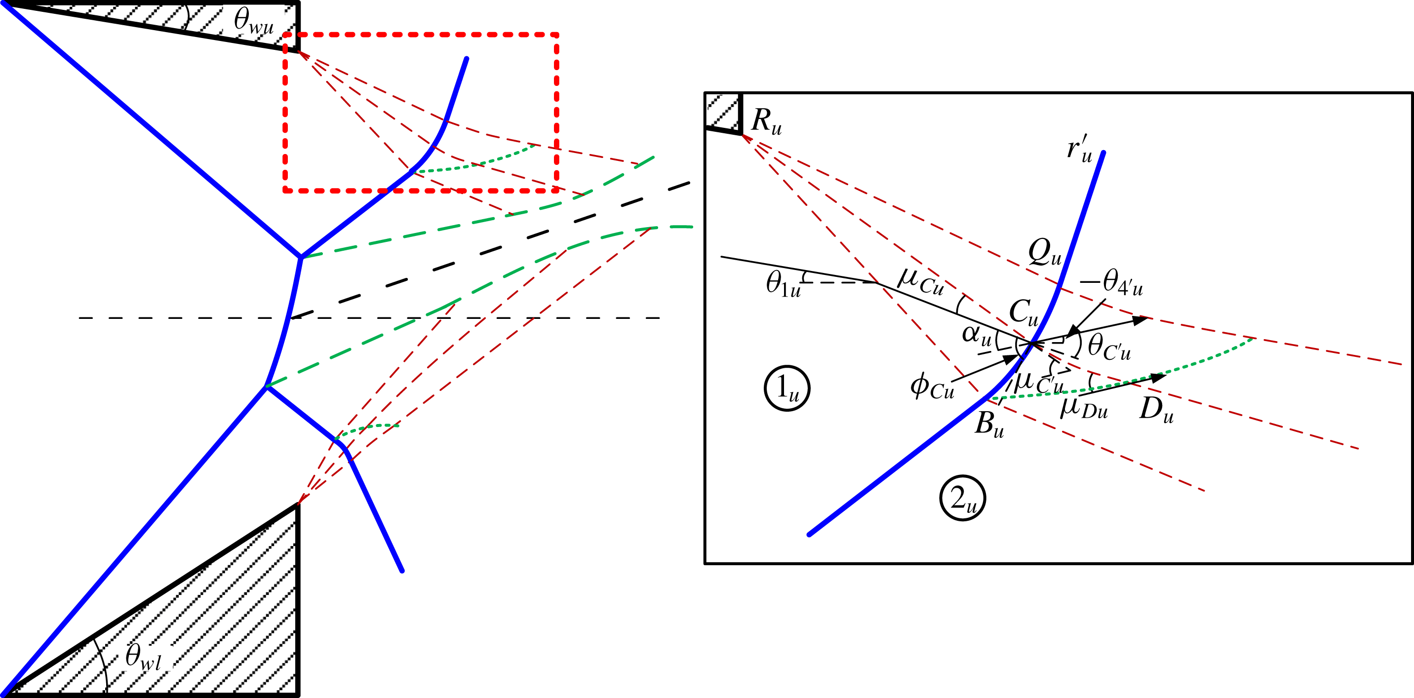
Figure 12. Schematic of asymmetric MR: inset; expansion fan interacting with reflected shock wave in upper domain.
Figure 13. Schematic of asymmetric MR: inset; expansion fan interacting with reflected shock wave in lower domain.
The regions of interaction of the expansion fans with the reflected shocks,
 $r$
, are given in figures 12 and 13. The inclination of the subsonic pocket (along axis
$r$
, are given in figures 12 and 13. The inclination of the subsonic pocket (along axis
 $x_{i}$
) by angle
$x_{i}$
) by angle
 $\unicode[STIX]{x1D703}_{4}$
is included as an angle correction, in the sense that the streamlines are shown to become parallel to
$\unicode[STIX]{x1D703}_{4}$
is included as an angle correction, in the sense that the streamlines are shown to become parallel to
 $x_{i}$
rather than
$x_{i}$
rather than
 $x$
, after interacting with a portion of the expansion fan (Li & Ben-Dor Reference Li and Ben-Dor1997; Ben-Dor Reference Ben-Dor2007). The slip line also follows the curvature of the weak tangential discontinuity (originating from point
$x$
, after interacting with a portion of the expansion fan (Li & Ben-Dor Reference Li and Ben-Dor1997; Ben-Dor Reference Ben-Dor2007). The slip line also follows the curvature of the weak tangential discontinuity (originating from point
 $B$
) which is one among an infinite number of such entropy layers. The pressure and flow direction remain constant across each layer. Details of the analytical study of expansion-fan interaction with a shock wave can be found in Li & Ben-Dor (Reference Li and Ben-Dor1996). Beyond the characteristic line
$B$
) which is one among an infinite number of such entropy layers. The pressure and flow direction remain constant across each layer. Details of the analytical study of expansion-fan interaction with a shock wave can be found in Li & Ben-Dor (Reference Li and Ben-Dor1996). Beyond the characteristic line
 $RCD$
of the centred expansion fan, where the flow for the most part assumes a common inclination
$RCD$
of the centred expansion fan, where the flow for the most part assumes a common inclination
 $\unicode[STIX]{x1D703}_{4}$
, further influence of the expansion fan is ignored as the flow downstream of the throat becomes supersonic and properties there do not influence the upstream flow any further.
$\unicode[STIX]{x1D703}_{4}$
, further influence of the expansion fan is ignored as the flow downstream of the throat becomes supersonic and properties there do not influence the upstream flow any further.
Consider the point where the characteristic line
 $RCD$
interacts with the reflected shock
$RCD$
interacts with the reflected shock
 $r$
. The point upstream of the shock is labelled as
$r$
. The point upstream of the shock is labelled as
 $C$
, and the point downstream as
$C$
, and the point downstream as
 $C^{\prime }$
. Here,
$C^{\prime }$
. Here,
 $\unicode[STIX]{x1D707}$
is the Mach angle made by the characteristic line at that point. The angle between the flow direction and axis
$\unicode[STIX]{x1D707}$
is the Mach angle made by the characteristic line at that point. The angle between the flow direction and axis
 $x_{i}$
at
$x_{i}$
at
 $C$
, is given as
$C$
, is given as
 $\unicode[STIX]{x1D6FC}$
.
$\unicode[STIX]{x1D6FC}$
.
Firstly, the Prandtl–Meyer relation is applied between a location in region 2 and point
 $D$
. The net change in the flow direction here is
$D$
. The net change in the flow direction here is
 $\unicode[STIX]{x1D703}_{3}-\unicode[STIX]{x1D703}_{4^{\prime }}$
, where
$\unicode[STIX]{x1D703}_{3}-\unicode[STIX]{x1D703}_{4^{\prime }}$
, where
 $\unicode[STIX]{x1D703}_{4^{\prime }}$
assumes the value of
$\unicode[STIX]{x1D703}_{4^{\prime }}$
assumes the value of
 $\unicode[STIX]{x1D703}_{4^{\prime }u}$
or
$\unicode[STIX]{x1D703}_{4^{\prime }u}$
or
 $\unicode[STIX]{x1D703}_{4^{\prime }l}$
as given in (3.8). The pressure remains constant across the parallel entropy layers. Hence, we have the following relations for
$\unicode[STIX]{x1D703}_{4^{\prime }l}$
as given in (3.8). The pressure remains constant across the parallel entropy layers. Hence, we have the following relations for
 $M_{D}$
,
$M_{D}$
,
 $P_{D}$
and
$P_{D}$
and
 $P_{C^{\prime }}$
.
$P_{C^{\prime }}$
.
 $$\begin{eqnarray}\displaystyle \unicode[STIX]{x1D703}_{3}-\unicode[STIX]{x1D703}_{4^{\prime }}=\unicode[STIX]{x1D708}(M_{D})-\unicode[STIX]{x1D708}(M_{2}),\quad P_{D}=P_{2}\unicode[STIX]{x1D712}(M_{2},M_{D}),\quad \text{and}\quad P_{C^{\prime }}=P_{D}, & & \displaystyle\end{eqnarray}$$
where
 $\unicode[STIX]{x1D708}$
is the Prandtl–Meyer function and
$\unicode[STIX]{x1D708}$
is the Prandtl–Meyer function and
 $\unicode[STIX]{x1D712}$
is an isentropic function relating the pressures across an expansion fan, given as follows,
$\unicode[STIX]{x1D712}$
is an isentropic function relating the pressures across an expansion fan, given as follows,
 $$\begin{eqnarray}\displaystyle & \displaystyle \unicode[STIX]{x1D708}(M)=\left(\frac{\unicode[STIX]{x1D6FE}+1}{\unicode[STIX]{x1D6FE}-1}\right)^{1/2}\arctan \left[\frac{(\unicode[STIX]{x1D6FE}-1)(M^{2}-1)}{\unicode[STIX]{x1D6FE}+1}\right]^{1/2}-\arctan (M^{2}-1)^{1/2} & \displaystyle\end{eqnarray}$$
 $$\begin{eqnarray}\displaystyle & \displaystyle \unicode[STIX]{x1D712}(M_{i},M_{j})=\left[\frac{2+(\unicode[STIX]{x1D6FE}-1)M_{i}^{2}}{2+(\unicode[STIX]{x1D6FE}-1)M_{j}^{2}}\right]^{\unicode[STIX]{x1D6FE}/(\unicode[STIX]{x1D6FE}-1)}. & \displaystyle\end{eqnarray}$$
Now, consider a location in region 1, and point
 $C$
. The Prandtl–Meyer function can be applied again for a change in flow direction by angle
$C$
. The Prandtl–Meyer function can be applied again for a change in flow direction by angle
 $\unicode[STIX]{x1D703}_{1}-(\unicode[STIX]{x1D6FC}+\unicode[STIX]{x1D703}_{4^{\prime }})$
. Standard relations can be applied across shock
$\unicode[STIX]{x1D703}_{1}-(\unicode[STIX]{x1D6FC}+\unicode[STIX]{x1D703}_{4^{\prime }})$
. Standard relations can be applied across shock
 $r$
at points
$r$
at points
 $C$
and
$C$
and
 $C^{\prime }$
. Hence, the following set of 6 equations are solved for the 6 remaining unknowns:
$C^{\prime }$
. Hence, the following set of 6 equations are solved for the 6 remaining unknowns:
 $M_{C}$
,
$M_{C}$
,
 $M_{C^{\prime }}$
,
$M_{C^{\prime }}$
,
 $P_{C}$
,
$P_{C}$
,
 $\unicode[STIX]{x1D719}_{C}$
,
$\unicode[STIX]{x1D719}_{C}$
,
 $\unicode[STIX]{x1D703}_{C^{\prime }}$
and
$\unicode[STIX]{x1D703}_{C^{\prime }}$
and
 $\unicode[STIX]{x1D6FC}$
.
$\unicode[STIX]{x1D6FC}$
.
 $$\begin{eqnarray}\displaystyle \unicode[STIX]{x1D708}(M_{C})-\unicode[STIX]{x1D708}(M_{1})=\unicode[STIX]{x1D703}_{1}-(\unicode[STIX]{x1D6FC}+\unicode[STIX]{x1D703}_{4^{\prime }}),\quad P_{C}=P_{1}\unicode[STIX]{x1D712}(M_{1},M_{C}), & & \displaystyle\end{eqnarray}$$
 $$\begin{eqnarray}\displaystyle M_{C^{\prime }}=F(M_{C},\unicode[STIX]{x1D719}_{C}),\quad P_{C^{\prime }}=P_{C}H(M_{C},\unicode[STIX]{x1D719}_{C}), & & \displaystyle\end{eqnarray}$$
 $$\begin{eqnarray}\displaystyle \unicode[STIX]{x1D703}_{C^{\prime }}=G(M_{C},\unicode[STIX]{x1D719}_{C}),\quad \text{and}\quad \unicode[STIX]{x1D6FC}=\unicode[STIX]{x1D703}_{C^{\prime }}. & & \displaystyle\end{eqnarray}$$
The flow parameters calculated herewith, can now be applied to solve for the geometrical relations.
3.4 Flow in the subsonic pocket and geometrical relations
The boundary conditions at the interface apply to both the upper and lower domains, and hence the set of equations in this subsection have to be solved simultaneously.
Consider the subsonic pocket
 $TFEKG$
in figure 9. Here, the cross-sectional area of the pocket at the Mach stem is approximated as the vertical height of the Mach stem
$TFEKG$
in figure 9. Here, the cross-sectional area of the pocket at the Mach stem is approximated as the vertical height of the Mach stem
 $H_{m}$
.
$H_{m}$
.
 $H_{s}$
is the perpendicular area of the cross-section at the throat i.e.
$H_{s}$
is the perpendicular area of the cross-section at the throat i.e.
 $EK$
. In order to evaluate
$EK$
. In order to evaluate
 $H_{s}$
, certain geometric manipulations are employed. The details of the geometric relations and the set of equations employed for this subsection are detailed in appendix A.
$H_{s}$
, certain geometric manipulations are employed. The details of the geometric relations and the set of equations employed for this subsection are detailed in appendix A.
It is to be noted here that the leading edges of the two wedges have been considered to have a horizontal gap
 $L$
and the same has been included while calculating the corresponding abscissae.
$L$
and the same has been included while calculating the corresponding abscissae.
 $L$
is to be set to zero where the leading edges are required to be at the same horizontal location.
$L$
is to be set to zero where the leading edges are required to be at the same horizontal location.
The quasi-one-dimensional analysis and the geometrical relations along with the closing equations, yield a total of 26 equations with 26 unknowns, including
 $H_{mu}$
and
$H_{mu}$
and
 $H_{ml}$
, from which we get the total height of the Mach stem.
$H_{ml}$
, from which we get the total height of the Mach stem.
 $$\begin{eqnarray}H_{mt}=H_{mu}+H_{ml}.\end{eqnarray}$$
Finally, the coordinates of the points obtained from the solution are used to reconstruct the entire oMR configuration. Further discussion on this is given in § 4.3.
4 Results and discussion
4.1 Symmetry case verification
Due to the nature of the algorithm used herein, the asymmetric MR formulation is expected to predict symmetric MR cases as well. Hence, the data of non-dimensional Mach stem height for symmetric MR are compared with those of the present model in table 1 and figure 14. It follows from symmetry that for equal upper and lower wedge angles, the shock reflection configuration for any mathematical model would be identical in the upper and lower domains. The comparison has hence been made with symmetric half-models by taking half of the height of the Mach stem
 $H_{mt}$
and that between the wedges
$H_{mt}$
and that between the wedges
 $H_{t}$
.
$H_{t}$
.
Table 1. Comparison of the non-dimensional Mach stem height,
 $H_{mt}/H_{t}$
, with the values from
$H_{mt}/H_{t}$
, with the values from
 $^{a}$
Li & Ben-Dor (Reference Li and Ben-Dor1997),
$^{a}$
Li & Ben-Dor (Reference Li and Ben-Dor1997),
 $^{b}$
Mouton & Hornung (Reference Mouton and Hornung2008) and
$^{b}$
Mouton & Hornung (Reference Mouton and Hornung2008) and
 $^{c}$
Gao & Wu (Reference Gao and Wu2010). All angles are in degrees.
$^{c}$
Gao & Wu (Reference Gao and Wu2010). All angles are in degrees.
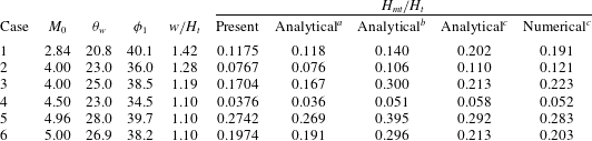
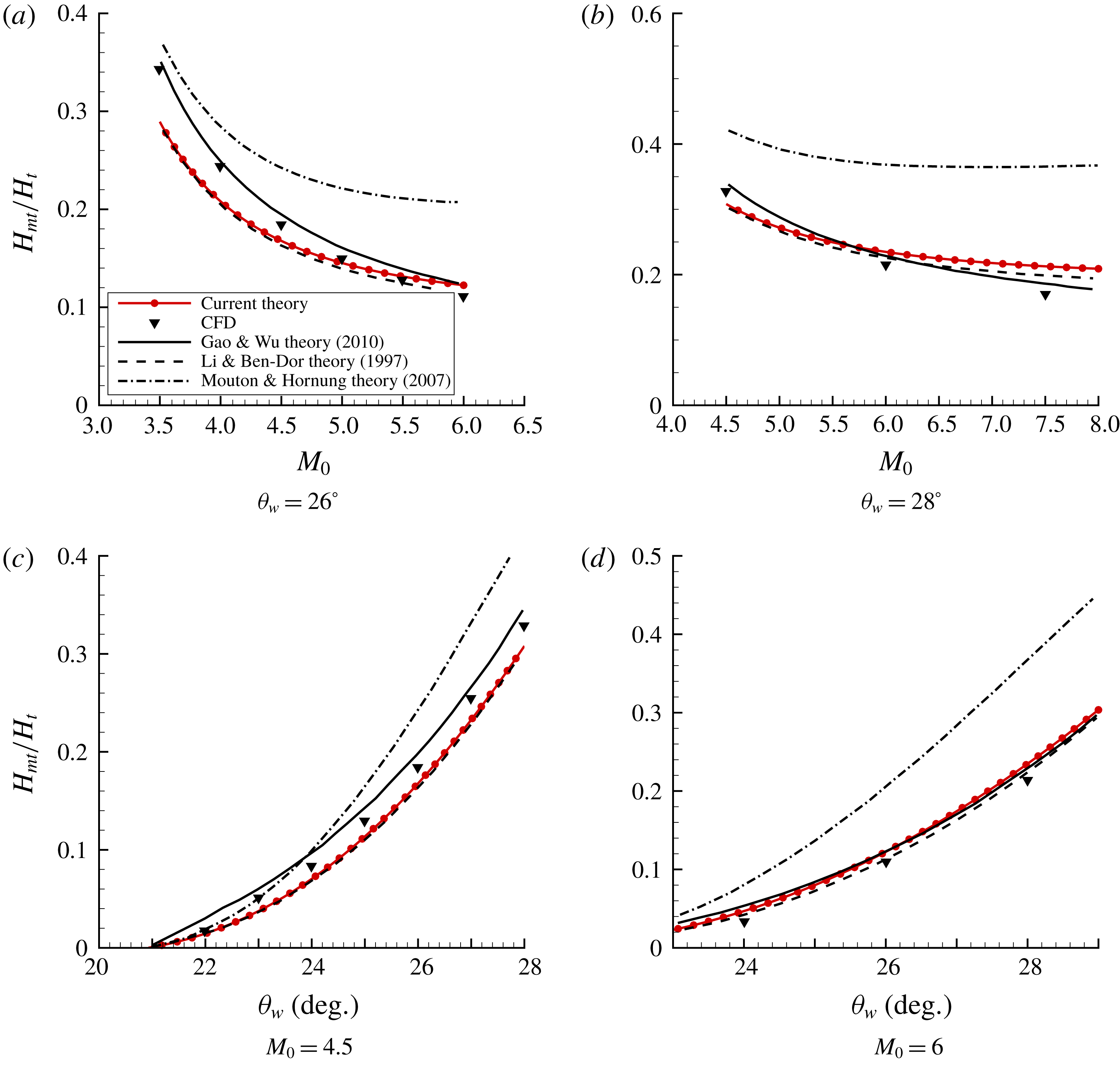
Figure 14. Comparisons of non-dimensional Mach stem height,
 $H_{mt}/H_{t}$
, from current theory with those of Gao & Wu (Reference Gao and Wu2010), Li & Ben-Dor (Reference Li and Ben-Dor1997) and Mouton & Hornung (Reference Mouton and Hornung2007), and numerical results from Gao & Wu (Reference Gao and Wu2010);
$H_{mt}/H_{t}$
, from current theory with those of Gao & Wu (Reference Gao and Wu2010), Li & Ben-Dor (Reference Li and Ben-Dor1997) and Mouton & Hornung (Reference Mouton and Hornung2007), and numerical results from Gao & Wu (Reference Gao and Wu2010);
 $w/H_{t}=1.1$
.
$w/H_{t}=1.1$
.
The data reported in table 1 and figure 14 are taken from Gao & Wu (Reference Gao and Wu2010). From table 1, it can be seen for cases 5 and 6 that the present model gives better, if not the best, agreement with the numerical data. From figure 14, it is evident that the present model (and that of Li & Ben-Dor (Reference Li and Ben-Dor1997)) shows excellent agreement with numerical results towards higher Mach numbers (
 $M_{0}>4.5$
). In selected cases, the present theory performs even better than that of Gao & Wu (Reference Gao and Wu2010). The Mouton (Reference Mouton2007) theory deviates from the numerical data at such high Mach numbers. At lower Mach numbers, there is considerable under-prediction of the Mach stem height by the present model. Since the primary distinction of the Gao & Wu (Reference Gao and Wu2010) model is the consideration of secondary waves in the MR configuration, the above analysis suggests that ignoring the secondary waves leads to large errors at low Mach numbers. However, the extent of their contribution at higher Mach numbers needs to be further considered, since we see very good agreement with the numerical data for a certain range, and some over-prediction beyond that (figure 14
a,b).
$M_{0}>4.5$
). In selected cases, the present theory performs even better than that of Gao & Wu (Reference Gao and Wu2010). The Mouton (Reference Mouton2007) theory deviates from the numerical data at such high Mach numbers. At lower Mach numbers, there is considerable under-prediction of the Mach stem height by the present model. Since the primary distinction of the Gao & Wu (Reference Gao and Wu2010) model is the consideration of secondary waves in the MR configuration, the above analysis suggests that ignoring the secondary waves leads to large errors at low Mach numbers. However, the extent of their contribution at higher Mach numbers needs to be further considered, since we see very good agreement with the numerical data for a certain range, and some over-prediction beyond that (figure 14
a,b).
It can also be noted from table 1 and figure 14 that there exists some discrepancy between the present data and those reported in Li & Ben-Dor (Reference Li and Ben-Dor1997). A closer scrutiny revealed a possible error in the algorithm reported in the latter (see Li & Ben-Dor Reference Li and Ben-Dor1997, C9, the appendix). The sign of the angle
 $\unicode[STIX]{x1D703}_{3}$
is incorrect, and the same has been corrected in the present theory in (A 12). It has separately been verified that for the symmetric case, the present asymmetric formulation gives exactly the same results as the corrected Li & Ben-Dor (Reference Li and Ben-Dor1997) model.
$\unicode[STIX]{x1D703}_{3}$
is incorrect, and the same has been corrected in the present theory in (A 12). It has separately been verified that for the symmetric case, the present asymmetric formulation gives exactly the same results as the corrected Li & Ben-Dor (Reference Li and Ben-Dor1997) model.
4.2 Variation of Mach stem height
Using the present algorithm, the wedge-angle-variation-induced changes in the Mach stem height have been estimated for a series of cases. Also, the wedge angles at which the Mach stem height becomes zero is in direct conformation to the von Neumann criterion. It is to be noted however that each value calculated using the present theory is a steady-state result. There is no dynamic effect (Naidoo & Skews Reference Naidoo and Skews2014) associated with changing wedge angles in this analytical model.
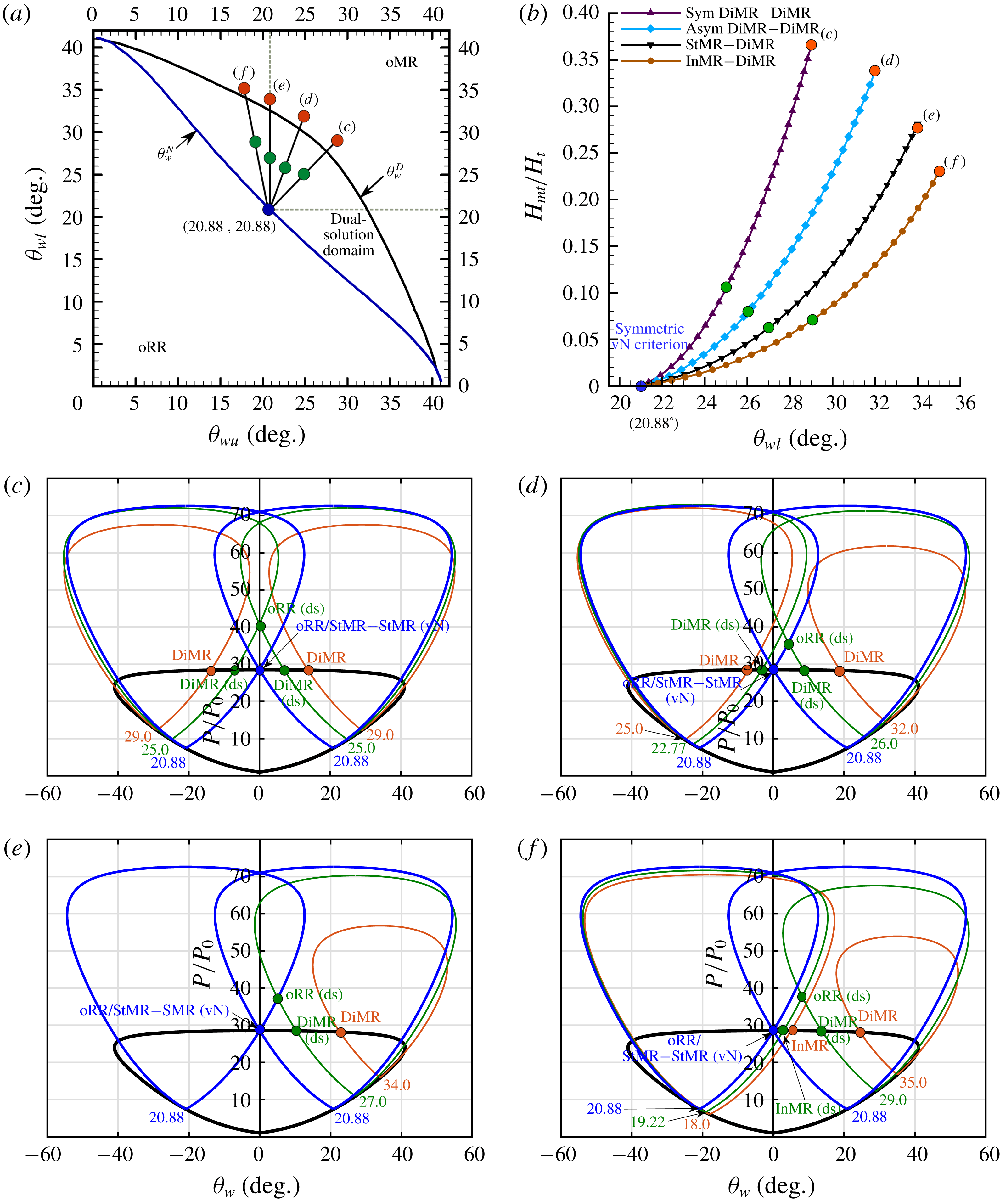
Figure 15. Symmetric von Neumann criterion for
 $M_{0}=4.96$
. (a) The dual-solution domain in the (
$M_{0}=4.96$
. (a) The dual-solution domain in the (
 $\unicode[STIX]{x1D703}_{wu}$
,
$\unicode[STIX]{x1D703}_{wu}$
,
 $\unicode[STIX]{x1D703}_{wl}$
)-plane (Li et al.
Reference Li, Chpoun and Ben-Dor1999); (b) plots of normalised Mach stem height versus lower wedge angle; (c) shock polars for symmetric DiMR–DiMR case; (d) shock polars for asymmetric DiMR-DiMR case; (e) shock polars for asymmetric StMR-DiMR; (f) shock polars for asymmetric InMR-DiMR case.
$\unicode[STIX]{x1D703}_{wl}$
)-plane (Li et al.
Reference Li, Chpoun and Ben-Dor1999); (b) plots of normalised Mach stem height versus lower wedge angle; (c) shock polars for symmetric DiMR–DiMR case; (d) shock polars for asymmetric DiMR-DiMR case; (e) shock polars for asymmetric StMR-DiMR; (f) shock polars for asymmetric InMR-DiMR case.
For all calculations in this subsection, the Mach number
 $M_{0}$
has been taken to be 4.96. The geometric parameters have been taken following Li et al. (Reference Li, Chpoun and Ben-Dor1999). The vertical height between the wedges is 71 mm and the wedges are of equal slant height at 40 mm each. The total pressure is taken to be 8.5 bar and the total temperature is 473 K. (These parameters are required as input to the algorithm. However, except the Mach number and geometrical parameters, other flow properties are dealt with as ratios across the discontinuities, and can be arbitrarily assumed within the perfect and ideal gas assumptions.) The above parameters ensure that oMR is possible for a range of angles in such a flow field, as determined from experimental results. The horizontal gap
$M_{0}$
has been taken to be 4.96. The geometric parameters have been taken following Li et al. (Reference Li, Chpoun and Ben-Dor1999). The vertical height between the wedges is 71 mm and the wedges are of equal slant height at 40 mm each. The total pressure is taken to be 8.5 bar and the total temperature is 473 K. (These parameters are required as input to the algorithm. However, except the Mach number and geometrical parameters, other flow properties are dealt with as ratios across the discontinuities, and can be arbitrarily assumed within the perfect and ideal gas assumptions.) The above parameters ensure that oMR is possible for a range of angles in such a flow field, as determined from experimental results. The horizontal gap
 $L$
between the wedges is zero.
$L$
between the wedges is zero.
In figure 15, the transitions from
 $\text{oMR}\rightarrow \text{oRR}$
have been shown for various types of initial oMR configurations. The cases taken here are symmetric DiMR–DiMR with equal wedge angles changing along the path
$\text{oMR}\rightarrow \text{oRR}$
have been shown for various types of initial oMR configurations. The cases taken here are symmetric DiMR–DiMR with equal wedge angles changing along the path
 $(c)$
, asymmetric DiMR–DiMR with unequal wedge angles varying along a straight line path
$(c)$
, asymmetric DiMR–DiMR with unequal wedge angles varying along a straight line path
 $(d)$
, StMR–DiMR with constant upper wedge angle (symmetric
$(d)$
, StMR–DiMR with constant upper wedge angle (symmetric
 $\unicode[STIX]{x1D703}_{w}^{N}$
) and varying lower wedge angle along the path
$\unicode[STIX]{x1D703}_{w}^{N}$
) and varying lower wedge angle along the path
 $(e)$
and, lastly, InMR–DiMR with unequal wedge angles varying along the straight line path
$(e)$
and, lastly, InMR–DiMR with unequal wedge angles varying along the straight line path
 $(f)$
. Figures 15(c) through 15(f) represent shock polars for the paths as indicated in figure 15(a), and the normalised Mach stem heights versus the lower wedge angles for these cases are given in figure 15(b). Solution points have been marked in colour in all the corresponding plots for each of the cases – only oMR, dual-solution (ds) domain and von Neumann (vN) criterion. A global sign convention for wedge angles is adopted for the shock polars here, whereby anticlockwise rotation as for the lower wedge is taken to be positive, and clockwise rotation as for the upper wedge is taken to be negative.
$(f)$
. Figures 15(c) through 15(f) represent shock polars for the paths as indicated in figure 15(a), and the normalised Mach stem heights versus the lower wedge angles for these cases are given in figure 15(b). Solution points have been marked in colour in all the corresponding plots for each of the cases – only oMR, dual-solution (ds) domain and von Neumann (vN) criterion. A global sign convention for wedge angles is adopted for the shock polars here, whereby anticlockwise rotation as for the lower wedge is taken to be positive, and clockwise rotation as for the upper wedge is taken to be negative.
All the plots in figure 15 converge at the symmetric von Neumann point, which for
 $M_{0}$
of 4.96 occurs at
$M_{0}$
of 4.96 occurs at
 $20.88^{\circ }$
. There is excellent agreement of the analytically predicted value as confirmed from theory from the (
$20.88^{\circ }$
. There is excellent agreement of the analytically predicted value as confirmed from theory from the (
 $\unicode[STIX]{x1D703}_{wu},\unicode[STIX]{x1D703}_{wl}$
)-plane and the shock polars. It is interesting to note that both the wedge angles would be equal at the symmetric von Neumann point, and this point hence, is a theoretical StMR–StMR configuration. However, the Mach stem height is zero at this point, and this denotes a transition to oRR.
$\unicode[STIX]{x1D703}_{wu},\unicode[STIX]{x1D703}_{wl}$
)-plane and the shock polars. It is interesting to note that both the wedge angles would be equal at the symmetric von Neumann point, and this point hence, is a theoretical StMR–StMR configuration. However, the Mach stem height is zero at this point, and this denotes a transition to oRR.
It is interesting to note from figure 15(b) that the highest Mach stem heights are obtained for the symmetric case, and the Mach stem heights for corresponding lower wedge angles become smaller as one moves away from symmetry. It is easy to extrapolate from symmetry that plots on the other side of symmetry line
 $(c)$
in the
$(c)$
in the
 $(\unicode[STIX]{x1D703}_{wu},\unicode[STIX]{x1D703}_{wl})$
-plane would bear the same pattern.
$(\unicode[STIX]{x1D703}_{wu},\unicode[STIX]{x1D703}_{wl})$
-plane would bear the same pattern.
It is also plausible to comment from this analysis that any approximation of an asymmetric MR to a symmetric MR (concept of equivalence shock angle, (Mouton Reference Mouton2007, chap. 5, 9)) would result in estimation of Mach stem height higher than the actual value. To elucidate this, table 2 lists the Mach stem heights for the various types of oMRs on paths
 $d$
,
$d$
,
 $e$
and
$e$
and
 $f$
, and those for the corresponding equivalence shock angle on path
$f$
, and those for the corresponding equivalence shock angle on path
 $c$
, in figure 15(b). It is seen that the difference increases with asymmetry, with the highest for InMR. For near-symmetric wedge angles as in the DiMR case, however, the difference is quite small, corroborating that proposed in Mouton (Reference Mouton2007).
$c$
, in figure 15(b). It is seen that the difference increases with asymmetry, with the highest for InMR. For near-symmetric wedge angles as in the DiMR case, however, the difference is quite small, corroborating that proposed in Mouton (Reference Mouton2007).
Table 2. Comparison of the non-dimensional Mach stem height,
 $H_{mt}/H_{t}$
, from the present theory for various asymmetric cases with corresponding symmetric case, based on the equivalence shock angle concept (Mouton Reference Mouton2007). All angles are in degrees.
$H_{mt}/H_{t}$
, from the present theory for various asymmetric cases with corresponding symmetric case, based on the equivalence shock angle concept (Mouton Reference Mouton2007). All angles are in degrees.

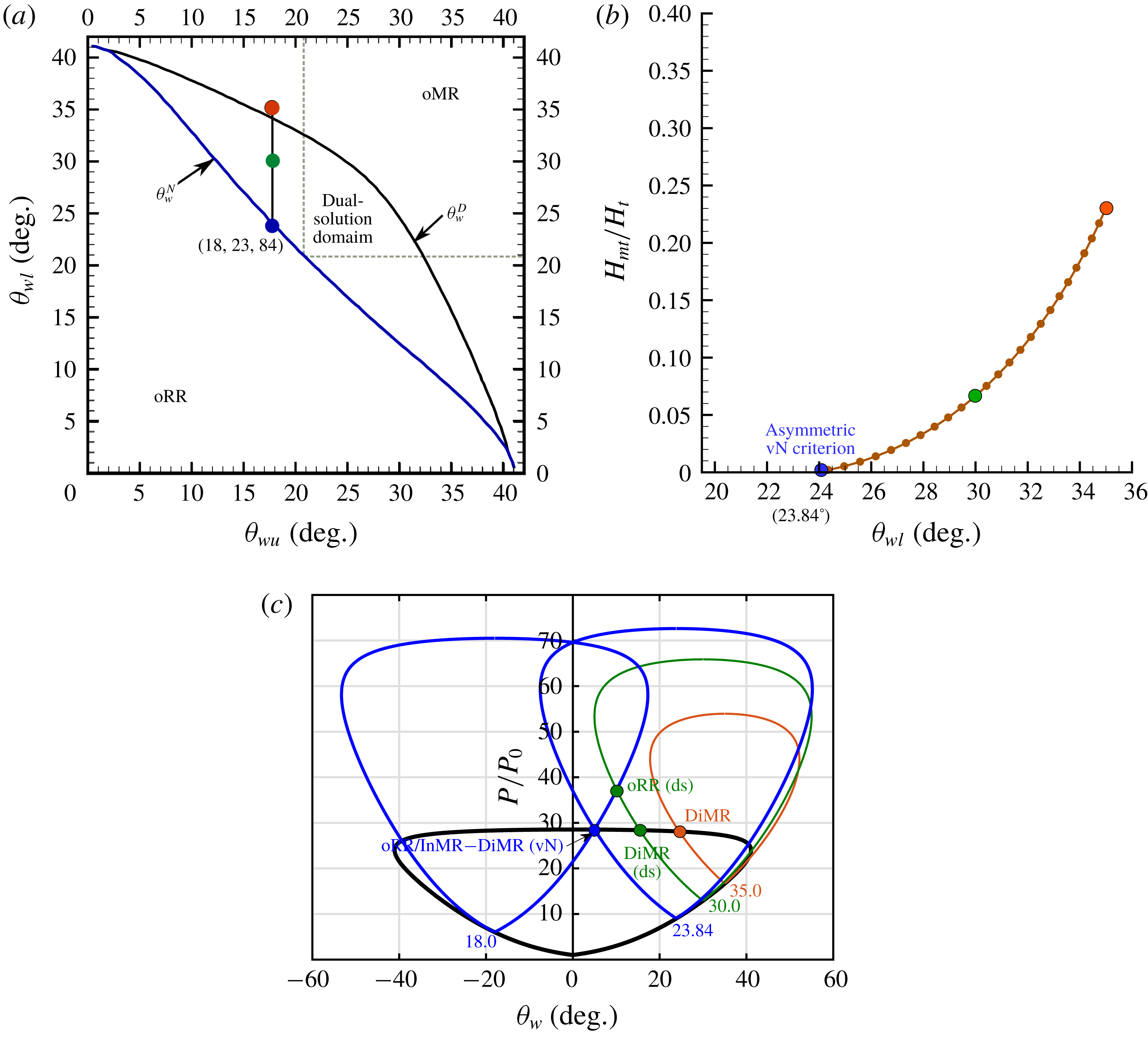
Figure 16. Asymmetric von Neumann criterion for
 $M_{0}=4.96$
. (a) The dual-solution domain in the (
$M_{0}=4.96$
. (a) The dual-solution domain in the (
 $\unicode[STIX]{x1D703}_{wu},\unicode[STIX]{x1D703}_{wl}$
)-plane (Li et al.
Reference Li, Chpoun and Ben-Dor1999); (b) plot of normalised Mach stem height versus lower wedge angle for InMR-DiMR; (c) shock polars for asymmetric InMR-DiMR case.
$\unicode[STIX]{x1D703}_{wu},\unicode[STIX]{x1D703}_{wl}$
)-plane (Li et al.
Reference Li, Chpoun and Ben-Dor1999); (b) plot of normalised Mach stem height versus lower wedge angle for InMR-DiMR; (c) shock polars for asymmetric InMR-DiMR case.
The salient feature of this work is the prediction of the InMR configurations. To see how accurate the present model predicts these configurations, cases of InMR–DiMR have been considered here in figure 16, whereby the upper wedge angle is retained at
 $18^{\circ }$
and the lower wedge angle is reduced until the von Neumann condition at
$18^{\circ }$
and the lower wedge angle is reduced until the von Neumann condition at
 $23.84^{\circ }$
. The path is shown on the (
$23.84^{\circ }$
. The path is shown on the (
 $\unicode[STIX]{x1D703}_{wu},\unicode[STIX]{x1D703}_{wl}$
)-plane in figure 16(a), the Mach stem height in figure 16(b), and the corresponding shock polars in figure 16(c). It can be seen that the von Neumann condition is accurately predicted at
$\unicode[STIX]{x1D703}_{wu},\unicode[STIX]{x1D703}_{wl}$
)-plane in figure 16(a), the Mach stem height in figure 16(b), and the corresponding shock polars in figure 16(c). It can be seen that the von Neumann condition is accurately predicted at
 $\unicode[STIX]{x1D703}_{wl}$
of
$\unicode[STIX]{x1D703}_{wl}$
of
 $23.84^{\circ }$
, as obtained from the shock polar theory.
$23.84^{\circ }$
, as obtained from the shock polar theory.
4.3 Asymmetric MR configurations
The coordinates of various points obtained as solutions from the algorithm are used to render the oMR configuration. Here, (2.1) is used to interpolate points for the curved entities – Mach stem, and portions of the slip lines, expansion-fan characteristic lines and reflected shocks.
The configuration obtained from the present model has been validated with numerical and experimental results in this section. As mentioned earlier, cases of highly asymmetric configurations such as those of InMR, are especially considered.
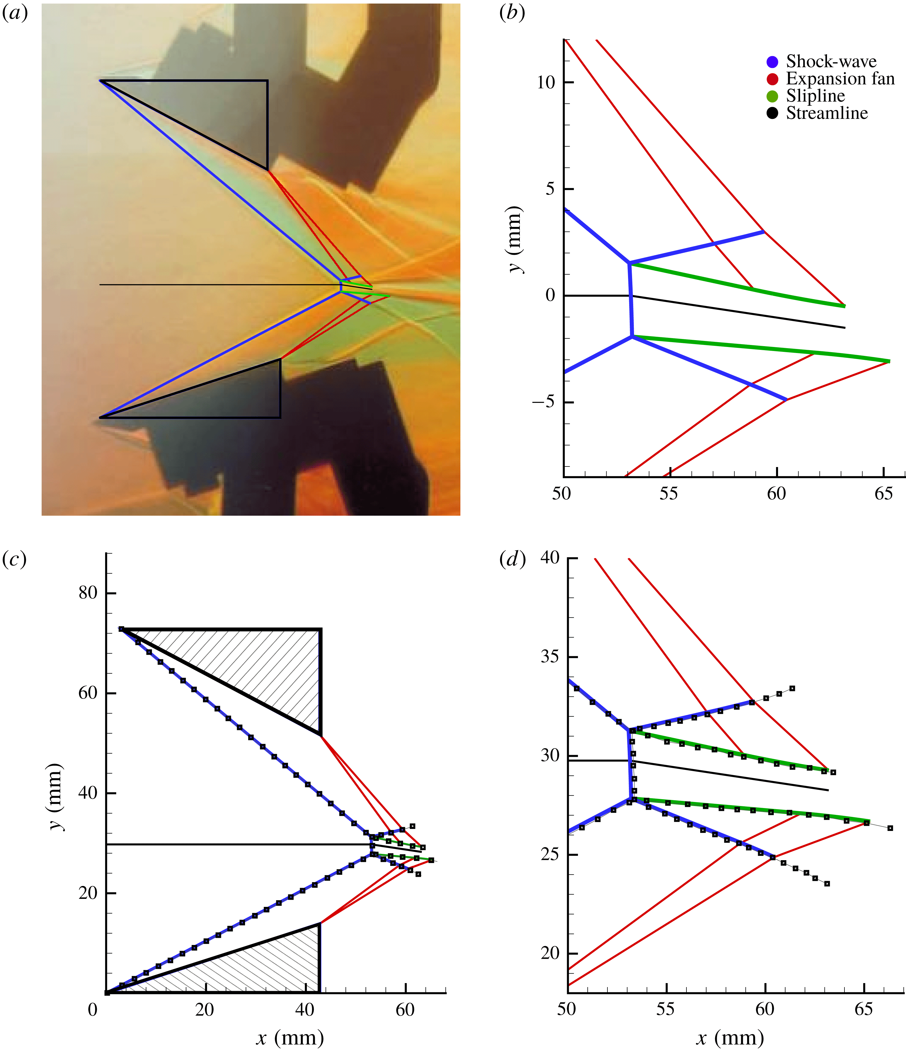
Figure 17. Comparison of inverse Mach reflection (DiMR–InMR) configuration at
 $M_{0}=4.96$
for
$M_{0}=4.96$
for
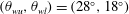 $(\unicode[STIX]{x1D703}_{wu},\unicode[STIX]{x1D703}_{wl})=(28^{\circ },18^{\circ })$
with present model (line plot). (a) Comparison with colour schlieren (Li et al.
Reference Li, Chpoun and Ben-Dor1999); (b) zoomed-in view of the Mach stem region; (c) comparison with data from numerical results, marked with ▫ (Ivanov et al.
Reference Ivanov, Ben-Dor, Elperin, Kudryavtsev and Khotyanovsky2002); (d) zoomed-in view of the Mach stem region in plot c.
$(\unicode[STIX]{x1D703}_{wu},\unicode[STIX]{x1D703}_{wl})=(28^{\circ },18^{\circ })$
with present model (line plot). (a) Comparison with colour schlieren (Li et al.
Reference Li, Chpoun and Ben-Dor1999); (b) zoomed-in view of the Mach stem region; (c) comparison with data from numerical results, marked with ▫ (Ivanov et al.
Reference Ivanov, Ben-Dor, Elperin, Kudryavtsev and Khotyanovsky2002); (d) zoomed-in view of the Mach stem region in plot c.

Figure 18. Comparison of oMR configurations with present model (line plot) with data from numerical results for
 $M_{0}=4.96$
, marked with ▫ (Ivanov et al.
Reference Ivanov, Ben-Dor, Elperin, Kudryavtsev and Khotyanovsky2002).
$M_{0}=4.96$
, marked with ▫ (Ivanov et al.
Reference Ivanov, Ben-Dor, Elperin, Kudryavtsev and Khotyanovsky2002).
In figure 17, the plots corresponding to an inverse Mach reflection, in particular oMR(DiMR
 $+$
InMR), for an upper wedge angle
$+$
InMR), for an upper wedge angle
 $\unicode[STIX]{x1D703}_{wu}$
of
$\unicode[STIX]{x1D703}_{wu}$
of
 $28^{\circ }$
and lower wedge angle
$28^{\circ }$
and lower wedge angle
 $\unicode[STIX]{x1D703}_{wl}$
of
$\unicode[STIX]{x1D703}_{wl}$
of
 $18^{\circ }$
, are shown. The wedge angles chosen correspond to an InMR–DiMR in the dual-solution domain on the (
$18^{\circ }$
, are shown. The wedge angles chosen correspond to an InMR–DiMR in the dual-solution domain on the (
 $\unicode[STIX]{x1D703}_{wu},\unicode[STIX]{x1D703}_{wl}$
)-plane, as can be seen from figure 16(a). In figure 17(a), the predicted configuration has been overlapped upon a colour schlieren photograph of an oMR for the same wedge angles, given in Li et al. (Reference Li, Chpoun and Ben-Dor1999). It can be seen that the predicted oMR configuration matches very well with the experimental oMR configuration. The rather small size of the Mach stem makes it difficult to visualise the area close to the stem. A zoomed-in view is therefore presented in figure 17(b). The line plots for various features such as shocks, characteristic lines of the expansion fan, slip line and streamline, are differentiated with colour. (The coordinate system shown in figure 17(b) corresponds to the approach primarily adopted in the present algorithm. For the latter plots, the axes have been shifted vertically down by
$\unicode[STIX]{x1D703}_{wu},\unicode[STIX]{x1D703}_{wl}$
)-plane, as can be seen from figure 16(a). In figure 17(a), the predicted configuration has been overlapped upon a colour schlieren photograph of an oMR for the same wedge angles, given in Li et al. (Reference Li, Chpoun and Ben-Dor1999). It can be seen that the predicted oMR configuration matches very well with the experimental oMR configuration. The rather small size of the Mach stem makes it difficult to visualise the area close to the stem. A zoomed-in view is therefore presented in figure 17(b). The line plots for various features such as shocks, characteristic lines of the expansion fan, slip line and streamline, are differentiated with colour. (The coordinate system shown in figure 17(b) corresponds to the approach primarily adopted in the present algorithm. For the latter plots, the axes have been shifted vertically down by
 $H_{l}$
.)
$H_{l}$
.)
It may be noted that the streamline direction downstream of the Mach stem is fictitious, as the flow is no longer uniform. The streamline represents the general flow direction and inclination of the subsonic pocket, or more correctly, axis
 $x_{i}$
of the present model. The slip lines become parallel to
$x_{i}$
of the present model. The slip lines become parallel to
 $x_{i}$
at their respective choking sections (part of the boundary conditions in the model) which is reasonable in the context of the experimental observations of such flow fields.
$x_{i}$
at their respective choking sections (part of the boundary conditions in the model) which is reasonable in the context of the experimental observations of such flow fields.
In figure 17(c,d), the predicted results have been compared with numerical data presented in Ivanov et al. (Reference Ivanov, Ben-Dor, Elperin, Kudryavtsev and Khotyanovsky2002). Here, the trailing edges of the two wedges are at the same horizontal location, unlike the leading edges as in the case of Li et al. (Reference Li, Chpoun and Ben-Dor1999). The two data sets have been scaled and mapped by matching the leading and trailing edges of the wedges. The agreement is seen to be quite good, with a clearer picture being provided by the magnified view.
The present model is known to predict a discontinuity between the upper and lower sections at the choking location. This is likely to become predominant at large asymmetric wedge angles owing the deviation from the quasi one-dimensional assumption used in the present formulation. However, it can be seen from the plots that the agreement between the computational and analytical data is quite good despite the fact that the asymmetry in wedge angles is large, indicating the reliability of the present model even for highly distorted oMR configurations.
Further cases of asymmetric MR have been given in figure 18, to compare the profiles of the present configurations with numerical results of Ivanov et al. (Reference Ivanov, Ben-Dor, Elperin, Kudryavtsev and Khotyanovsky2002). Figure 18(a) shows a direct MR (DiMR–DiMR) case with
 $(\unicode[STIX]{x1D703}_{wu},\unicode[STIX]{x1D703}_{wl})$
as (
$(\unicode[STIX]{x1D703}_{wu},\unicode[STIX]{x1D703}_{wl})$
as (
 $28^{\circ },30^{\circ }$
). The oMR configuration is more asymmetric in figure 18(b), but the configuration is still a direct MR. Figure 18(c) shows a case of stationary MR (DiMR–StMR), whereby the slip line for the lower domain emerges parallel to the incoming flow direction at the triple point. Lastly, figure 18(d) shows an inverse MR (InMR–DiMR) with a substantial height of the Mach stem. This configuration clearly reveals the profile of the Mach stem. The agreement with the numerical data is excellent for the above cases, though close inspection reveals that the present model under-predicts the Mach stem height by a small margin for cases (
$28^{\circ },30^{\circ }$
). The oMR configuration is more asymmetric in figure 18(b), but the configuration is still a direct MR. Figure 18(c) shows a case of stationary MR (DiMR–StMR), whereby the slip line for the lower domain emerges parallel to the incoming flow direction at the triple point. Lastly, figure 18(d) shows an inverse MR (InMR–DiMR) with a substantial height of the Mach stem. This configuration clearly reveals the profile of the Mach stem. The agreement with the numerical data is excellent for the above cases, though close inspection reveals that the present model under-predicts the Mach stem height by a small margin for cases (
 $a$
), (
$a$
), (
 $b$
) and (
$b$
) and (
 $c$
), while slightly over-predicting for case (
$c$
), while slightly over-predicting for case (
 $d$
). The Mach stem profile is accurately captured, as seen in cases (
$d$
). The Mach stem profile is accurately captured, as seen in cases (
 $a$
) and (
$a$
) and (
 $d$
).
$d$
).
5 Conclusion
The analytical formulation presented in this paper predicts the overall configuration of an asymmetric Mach reflection for all the possible oMR configurations. The model successfully predicts the profile of the waves and wave interactions in the oMR configurations. The present model takes into account most of the flow phenomena, such as the curved Mach stem, subsonic pocket and the interaction of the reflected shocks with the expansion fans, that occur in the shock reflections in the asymmetric wedge flows. The Mach stem heights predicted by the model have been validated with several numerical and analytical data available for symmetric cases. The agreement is quite good at high Mach numbers. However, the effects of ignoring secondary waves in the present model at very high Mach numbers need to be further investigated.
The asymmetric Mach stem heights have been computed for various types of oMR configurations. The pattern of variation of Mach stem height with wedge angles, for a Mach number of 4.96, is explored. The von Neumann criterion is found to be satisfied exactly by the present model for both symmetric and asymmetric cases. The highest Mach stem height is obtained when approached on the symmetric path. This suggests that equivalence angles, as employed in some of the previous works to approximate the asymmetric case to symmetric case, will result in over-prediction of the Mach stem height, although the difference is minimal for small asymmetries.
The profile of the overall asymmetric MR configuration is predicted and validated for a Mach number of 4.96 with experimental and numerical data. It is seen that the present model is able to predict the MR configuration with appreciable accuracy. The Mach stem profile is well captured in all cases, including inverse MR.
Appendix A
A.1 Flow in the subsonic pocket and geometrical relations
A schematic of the upper domain with the necessary nomenclature is given in figure 19. The lower domain follows a similar description. From figure 19, the following relations are evident based on the geometry. The abscissa of the leading edge of the lower wedge is the same as the origin on the
 $x$
axis. The upper wedge is at a horizontal gap
$x$
axis. The upper wedge is at a horizontal gap
 $L$
, as shown.
$L$
, as shown.
 $$\begin{eqnarray}\displaystyle \left.\begin{array}{@{}c@{}}\displaystyle X_{Au}=L,\quad X_{Al}=0.0,\quad X_{Ru}=L+w_{u}\cos \unicode[STIX]{x1D703}_{1u},\quad X_{Rl}=w_{l}\cos \unicode[STIX]{x1D703}_{1l},\\ X_{Tu}=L+(H_{u}-H_{mu})\cot \unicode[STIX]{x1D719}_{1u},\quad X_{Tl}=(H_{l}-H_{ml})\cot \unicode[STIX]{x1D719}_{1l},\\ Y_{R}=H-w\sin \unicode[STIX]{x1D703}_{1},\quad \text{and}\quad Y_{T}=H_{m}.\end{array}\right\} & & \displaystyle\end{eqnarray}$$
Consider the subsonic pocket
 $TFEKG$
. The angle
$TFEKG$
. The angle
 $\unicode[STIX]{x1D6FD}$
is given by the inverse of the tangent of the ratio of
$\unicode[STIX]{x1D6FD}$
is given by the inverse of the tangent of the ratio of
 $EN$
and
$EN$
and
 $GN$
. By adding
$GN$
. By adding
 $\unicode[STIX]{x1D703}_{4^{\prime }}$
to
$\unicode[STIX]{x1D703}_{4^{\prime }}$
to
 $\unicode[STIX]{x1D6FD}$
(in case of the upper domain, adding
$\unicode[STIX]{x1D6FD}$
(in case of the upper domain, adding
 $\unicode[STIX]{x1D703}_{4^{\prime }u}=-\unicode[STIX]{x1D703}_{4}$
to
$\unicode[STIX]{x1D703}_{4^{\prime }u}=-\unicode[STIX]{x1D703}_{4}$
to
 $\unicode[STIX]{x1D6FD}_{u}$
), we get the angle
$\unicode[STIX]{x1D6FD}_{u}$
), we get the angle
 $\unicode[STIX]{x1D6FF}$
, from which
$\unicode[STIX]{x1D6FF}$
, from which
 $H_{s}$
can be obtained using a
$H_{s}$
can be obtained using a
 $\sin$
function along with the length
$\sin$
function along with the length
 $EG$
. The relations are given below.
$EG$
. The relations are given below.
 $$\begin{eqnarray}\left.\begin{array}{@{}c@{}}\displaystyle \unicode[STIX]{x1D6FD}=\text{atan}\left[\frac{Y_{E}}{X_{E}-X_{G}}\right],\quad \unicode[STIX]{x1D6FF}=\unicode[STIX]{x1D6FD}+\unicode[STIX]{x1D703}_{4^{\prime }},\\ \text{and}\quad H_{s}=\sqrt{(Y_{E})^{2}+(X_{E}-X_{G})^{2}}\sin \unicode[STIX]{x1D6FF}.\end{array}\right\}\end{eqnarray}$$
As mentioned at the beginning of § 3, the sonic contour is not taken to be continuous from
 $E_{u}$
to
$E_{u}$
to
 $E_{l}$
. Rather, the choking throats are approximated as straight cross-sectional areas, perpendicular to the axis
$E_{l}$
. Rather, the choking throats are approximated as straight cross-sectional areas, perpendicular to the axis
 $x_{i}$
, to be better suited to the quasi-one-dimensional assumption here. Results obtained by Roy & Rajesh (Reference Roy and Rajesh2017) show that the MR profile around the Mach stem is disoriented when the sonic contour is imposed to be a continuous straight or slightly curved line. Furthermore, adding boundary conditions of continuity for both the Mach stem and sonic contour over-constrains the set of equations in this subsection.
$x_{i}$
, to be better suited to the quasi-one-dimensional assumption here. Results obtained by Roy & Rajesh (Reference Roy and Rajesh2017) show that the MR profile around the Mach stem is disoriented when the sonic contour is imposed to be a continuous straight or slightly curved line. Furthermore, adding boundary conditions of continuity for both the Mach stem and sonic contour over-constrains the set of equations in this subsection.

Figure 19. Schematic of upper domain of asymmetric MR configuration.
The average Mach number downstream of the Mach stem
 $ms$
has been calculated in § 3.2.2. Using
$ms$
has been calculated in § 3.2.2. Using
 $\overline{M}$
, we apply the quasi-one-dimensional-area–Mach-number relation between
$\overline{M}$
, we apply the quasi-one-dimensional-area–Mach-number relation between
 $H_{m}$
and
$H_{m}$
and
 $H_{s}$
, as follows.
$H_{s}$
, as follows.
 $$\begin{eqnarray}\frac{H_{m}}{H_{s}}=\frac{1}{\overline{M}}\left[\frac{2}{\unicode[STIX]{x1D6FE}+1}\left(1+\frac{\unicode[STIX]{x1D6FE}-1}{2}\overline{M}^{2}\right)\right]^{(\unicode[STIX]{x1D6FE}+1)/2(\unicode[STIX]{x1D6FE}-1)}.\end{eqnarray}$$
We now advance with a more rigorous consideration of the geometric relations. Refer to figure 19 for the following.
Consider the straight line
 $RB$
,
$RB$
,
 $$\begin{eqnarray}Y_{B}-Y_{R}=-\tan (\unicode[STIX]{x1D707}_{B}+\unicode[STIX]{x1D703}_{1})(X_{B}-X_{R}),\quad \text{where }\unicode[STIX]{x1D707}_{B}=\arcsin (1/M_{1})\end{eqnarray}$$
consider the straight line
 $RC$
,
$RC$
,
 $$\begin{eqnarray}Y_{C}-Y_{R}=-\tan (\unicode[STIX]{x1D707}_{C}+\unicode[STIX]{x1D6FC}+\unicode[STIX]{x1D703}_{4^{\prime }})(X_{C}-X_{R}),\quad \text{where }\unicode[STIX]{x1D707}_{C}=\arcsin (1/M_{C})\end{eqnarray}$$
consider the straight line
 $BF$
,
$BF$
,
 $$\begin{eqnarray}Y_{F}-Y_{B}=-\tan (\unicode[STIX]{x1D707}_{F}+\unicode[STIX]{x1D703}_{3})(X_{F}-X_{B}),\quad \text{where }\unicode[STIX]{x1D707}_{F}=\arcsin (1/M_{2})\end{eqnarray}$$
consider the straight line
 $DE$
,
$DE$
,
 $$\begin{eqnarray}Y_{E}-Y_{D}=-\tan (\unicode[STIX]{x1D707}_{D}+\unicode[STIX]{x1D703}_{4^{\prime }})(X_{E}-X_{D}),\quad \text{where }\unicode[STIX]{x1D707}_{D}=\arcsin (1/M_{D})\end{eqnarray}$$
consider the straight line
 $TB$
,
$TB$
,
 $$\begin{eqnarray}Y_{B}-Y_{T}=\tan (\unicode[STIX]{x1D719}_{2}-\unicode[STIX]{x1D703}_{1})(X_{B}-X_{T})\end{eqnarray}$$
consider the straight line
 $TF$
,
$TF$
,
 $$\begin{eqnarray}Y_{F}-Y_{T}=-\tan \unicode[STIX]{x1D703}_{3}(X_{F}-X_{T}).\end{eqnarray}$$
For curved line segments, we take equations of the form given in (2.2), and use the function in (2.3). It is assumed here that these curvatures are very small. The profile of the curve is a function of the coordinates of its end points and the inclinations (slope with the
 $x$
-axis) of the curve at the end points.
$x$
-axis) of the curve at the end points.
Consider the curve
 $BC$
,
$BC$
,
 $$\begin{eqnarray}Y_{B}-Y_{C}=\tan \unicode[STIX]{x1D6EC}[(\unicode[STIX]{x1D719}_{2}-\unicode[STIX]{x1D703}_{1}),(\unicode[STIX]{x1D719}_{C}-\unicode[STIX]{x1D6FC}-\unicode[STIX]{x1D703}_{4^{\prime }})](X_{B}-X_{C})\end{eqnarray}$$
consider the curve
 $CD$
,
$CD$
,
 $$\begin{eqnarray}Y_{C}-Y_{D}=\tan \unicode[STIX]{x1D6EC}[(-\arcsin (1/M_{C^{\prime }})-\unicode[STIX]{x1D703}_{4^{\prime }}),(-\arcsin (1/M_{D})-\unicode[STIX]{x1D703}_{4^{\prime }})](X_{C}-X_{D})\end{eqnarray}$$
consider the curve
 $BD$
,
$BD$
,
 $$\begin{eqnarray}Y_{B}-Y_{D}=\tan \unicode[STIX]{x1D6EC}[(-\unicode[STIX]{x1D703}_{3}),(-\unicode[STIX]{x1D703}_{4^{\prime }})](X_{B}-X_{D})\end{eqnarray}$$
consider the curve
 $FE$
,
$FE$
,
 $$\begin{eqnarray}Y_{F}-Y_{E}=\tan \unicode[STIX]{x1D6EC}[(-\unicode[STIX]{x1D703}_{3}),(-\unicode[STIX]{x1D703}_{4^{\prime }})](X_{F}-X_{E}).\end{eqnarray}$$
The set of equations (A 3) to (A 13), considering both the domains, constitute a total of 22 equations and 26 unknowns. Additional equations for boundary conditions have to be added, to close the set of equations. Firstly, we know the relation for the total height between the wedges.
 $$\begin{eqnarray}H_{t}=H_{u}+H_{l}.\end{eqnarray}$$
As discussed earlier in § 2, following Roy & Rajesh (Reference Roy and Rajesh2017) we employ the condition that the Mach stem is required to have a continuous profile between the triple points in the upper and lower domains. Value of
 $\unicode[STIX]{x1D719}_{4}$
has already been obtained in § 3.2.1.
$\unicode[STIX]{x1D719}_{4}$
has already been obtained in § 3.2.1.
 $$\begin{eqnarray}Y_{T}=\tan \unicode[STIX]{x1D6EC}[(\unicode[STIX]{x03C0}-\unicode[STIX]{x1D719}_{3}),(\unicode[STIX]{x1D719}_{4^{\prime }})](X_{T}-X_{G}),\quad \text{where }\unicode[STIX]{x1D719}_{4^{\prime }u}=\unicode[STIX]{x1D719}_{4},\unicode[STIX]{x1D719}_{4^{\prime }l}=\unicode[STIX]{x03C0}-\unicode[STIX]{x1D719}_{4}.\end{eqnarray}$$
And,
 $$\begin{eqnarray}X_{Gu}=X_{Gl}.\end{eqnarray}$$
We now have a total of 26 equations (A 3) to (A 16) for the 26 unknowns (read for both upper
 $u$
and lower
$u$
and lower
 $l$
domains):
$l$
domains):
 $X_{G}$
,
$X_{G}$
,
 $Y_{T}$
,
$Y_{T}$
,
 $X_{B}$
,
$X_{B}$
,
 $Y_{B}$
,
$Y_{B}$
,
 $X_{C}$
,
$X_{C}$
,
 $Y_{C}$
,
$Y_{C}$
,
 $X_{D}$
,
$X_{D}$
,
 $Y_{D}$
,
$Y_{D}$
,
 $X_{F}$
,
$X_{F}$
,
 $Y_{F}$
,
$Y_{F}$
,
 $X_{E}$
,
$X_{E}$
,
 $Y_{E}$
and
$Y_{E}$
and
 $H$
. Here,
$H$
. Here,
 $H_{m}=Y_{T}$
, from which we get the total height of the Mach stem, and from
$H_{m}=Y_{T}$
, from which we get the total height of the Mach stem, and from
 $H$
we get the location of the
$H$
we get the location of the
 $x/x_{i}$
axes.
$x/x_{i}$
axes.


