


1. INTRODUCTION
Product configurators have a long history in artificial intelligence (AI; Sabin & Weigel, Reference Sabin and Weigel1998; Felfernig, Reference Felfernig2007), the first and most famous example being the rule-based configurator R1/XCON system (McDermott, Reference McDermott1982) for DEC-Computer. Today there are several established vendors of commercial configurators based on AI methods (SAP, Oracle, ILOG, Tacton, ConfigIt, etc.). Nevertheless, many products especially in technical domains are configured by engineers using in-house software without AI technology. A reason for this may be that there is little literature available on how to use AI methods specifically for product configuration. Therefore, this paper aims at readers with only limited AI background, who are interested in how to model and solve product configuration problems using AI methodologies. For the AI experts it provides insight into how to map a problem between the different paradigms (logic programming, object oriented, constraint based) and proposes a flexible software architecture for product configurators.
Product configurators for technical artifacts pose other challenges than product configurators for customer products. Customer products are typically designed for easy configurability and can be configured by the average customer. Configuring technical systems often requires an engineer with high domain knowledge. Depending on the business domain, various structural, physical, and chemical constraints, and so forth on the assembly of the system or product may arise. With their dependencies between several system components, those constraints can get quite complicated. Although algorithms for general-purpose solvers have been significantly improved over the last years (e.g., Cooper et al., Reference Cooper, Jeavons and Salamon2008), they turn out to be too inefficient in many cases (Mayer et al., Reference Mayer, Bettex, Stumptner, Falkner and Faltings2009). Then, problem-specific implementations seem necessary. Unfortunately, they also have drawbacks: their maintenance and adaptations to changing requirements are more difficult; often they require deep insight into the nature of the problem that an average knowledge engineer does not necessarily have.
Fortunately, over the last years many (often free) solvers suitable for real-world applications have been developed. In contrast to the monolithic AI systems of the past there is a trend to integrate relatively small specialized AI tools within conventional software systems. A typical example is SAT4J, a satisfiability library, which ships with every instance of the Eclipse integrated development environment (IDE) and is deployed on millions of computers. Most of the users of the Eclipse IDE are even unaware of the AI technology inside of Eclipse.
In the rest of this paper we show a typical product configuration problem as an example for such kinds of real-world problems as well as corresponding solution approaches using different AI methodologies. Section 2 describes a technical product configuration problem. Although seemingly simple, it poses hard efficiency demands on the solving process. In Section 3 an object-oriented model of the problem is derived and some of its properties are analyzed using Unified Modeling Language (UML)/Object Constraint Language (OCL), Alloy, and generative constraint satisfaction problem CSP. In Section 4 we present and evaluate different approaches for solving configuration problems. Section 5 gives a summary of the results and arrives at the conclusion that the challenge for the knowledge engineer consists not only in choosing the right solver(s) for the problem, but also in how to integrate the different solvers into one coherent system. Finally, Section 6 answers that question and proposes an architecture for integrating different solvers into a product configurator framework.
2. PROBLEM DESCRIPTION
The first step for developing a product configurator is the specification of the customer requirements, that is, the properties of the configurable product. As an example we use a fictitious people-counting system for museums. The structure of the problem is similar to problems we encountered in different real-world domains of our product configurators.
A museum has lots of rooms, and there are doors between some of them. In order to prevent damage to the objects in exhibition, the number of visitors shall be restricted. This is done by a people-counting system that consists of the following components: door sensors, counting zones, and communication units.
A door sensor detects everybody who moves through its door (directed movement detection). There can be doors without a sensor.
Any number of rooms may be grouped to a counting zone. Each zone knows how many persons are in it (counting the information from the sensors at doors leading outside of the zone—doors between rooms of the zone are ignored). Correct function requires that all doors leading outside a zone have a sensor (the corresponding constraint is not part of this problem). Zones may overlap or include other zones, that is, a room may be part of several zones.
A communication unit can control at most two door sensors and at most two zones. If a unit controls a sensor that contributes to a zone on another unit, then the two units need a direct connection: one is a partner unit of the other and vice versa. Each unit can have at most N partner units. For the sake of simplicity, we use N = 2 throughout this paper, whereas higher values for N are more common in real-life problems of this kind. Of course, the problem diminishes or even vanishes when N is chosen sufficiently high or unbounded, but we assume technical reasons inhibiting high values.
PartnerUnits problem: Given a consistent configuration of door sensors and zones, find a valid assignment of units (i.e., a maximum of two partners) striving for a minimal number of units.
Example 1: Rooms 1 to 8 with doors, eight of the doors having a door sensor, for example, there is a sensor between rooms 1 and 2, or 3 and 4, but not between 2 and 3 (Fig. 1).
Given zones: 1 (white), 2378 (light gray), 45 (dark gray), 6 (medium gray), 456, 2367, 2345678. They are consistent to the door sensors because all doors without sensors are only inside zones. The sensor between 7 and 8 is ignored for zones 2378 and 2345678, but necessary for zone 2367.

Fig. 1. The room layout of example 1.
The door sensors are named D01, D12, D26, D34, and so forth for the rooms that they connect (and 0 for the outside, respectively). The zones get their names from the rooms that they contain: Z1, Z2345678, Z2367, and so forth.
The relation between zones and door sensors, which is represented as a bipartite graph, is shown in Figure 2. A minimal solution using only four units is, for example, solution 1 in Table 1.
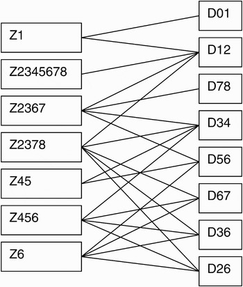
Fig. 2. The relation between zones and door sensors in example 1.
Table 1. A minimal solution of example 1

For small examples (i.e., less than six sensors and six zones), it is easy to find a solution. If the number of sensors for each zone is less than three and vice versa, a trivial but far from minimal solution would be to put each zone and each sensor onto a separate unit.
For bigger configurations, the constraint of maximal two partner units makes the problem hard. For example, adding zone Z23 (and new sensor D27) has no solution at all. However, adding Z18 to the free position on unit 4 is a solution. Even adding Z4 (and new sensor D45) has a solution with the minimally achievable number of five units, for example, solution 2 in Table 2.
Table 2. A minimal solution of extended example 1

In addition to finding a consistent solution to the PartnerUnits problem, the following questions may be asked:
• What is the minimal number of units needed? Clearly, the absolute minimum is the smallest integer greater or equal to the half of the maximum of the number of zones and the number of door sensors. However, we do not know whether there is always a solution with such few units.
• Given a partial assignment (i.e., not all sensors or zones have a unit yet), is there a valid extension?
• Reconfiguration: what is the minimal set of changes to already assigned units, so that a valid extension is possible? For example, given solution 1, add Z4 (and new sensor D45) and find a solution with minimal differences to solution 1, that is, change as few assignments to units as possible.
This paper concentrates on finding (preferably minimal) solutions. The other topics are subject to further research.
3. MODELING
After collecting the customer requirements of the product to be configured, the configurator designer must choose an appropriate language and tool for modeling the problem. A model consists of the representation of the configuration components as well as constraints and rules defining valid solutions. For many technical domains, the models get complex and large, so that a high-level modeling language is required. It provides for an easy, natural, and elegant problem description, supporting readability, validation, and maintainability of the model.
We demonstrate the modeling of the PartnerUnits problem prototypically by three languages: UML/OCL (http://www.omg.org/spec/UML/2.3, http://www.omg.org/spec/OCL/2.2), widely used as analysis and design specification language, Alloy (Jackson, Reference Jackson2002), a first-order logic language well suited for associations, and generative CSP (Fleischanderl et al., Reference Fleischanderl, Friedrich, Haselböck, Schreiner and Stumptner1998; Gottlob et al., Reference Gottlob, Greco and Mancini2007), which allows the formulation of dynamic problems like configuration as CSPs. For brevity reasons, we do not cover description logics in this article. Description logics is prominent for the formal representation and reasoning on the concepts of complex knowledge networks and is a wide research field in AI (see, e.g., Baader et al., Reference Baader, McGuinness, Nardi and Patel-Schneider2003; Felfernig et al., Reference Felfernig, Friedrich, Jannach, Stumptner and Zanker2003).
3.1. UML/OCL
UML class diagrams (Fig. 3) are a common way to describe the structure of a system in object-oriented modeling. The primary use of UML diagrams is to communicate the model visually inside a software project. In combination with OCL it is also expressive enough to describe product configuration (Felfernig et al., Reference Felfernig, Friedrich, Jannach and Zanker2002).

Fig. 3. UML diagram of class PartnerUnits.
The UML diagram shows a class diagram derived from the description. It contains the cardinality constraints, but there is no way to express the fact that the partner units association is derived from the path over the zone2sensor relation inside the class diagram. It must be expressed using an OCL constraint:
Let myPartnerUnitsSensor be the set of units reachable from a unit by navigating from its sensors to the zones and then their units (sensor.zone.unit), and let myPartnerUnitsZone be the set of units reachable by navigating from the zones to the sensors and then to the units (zone.sensor.unit). Then the cardinality of the union of myPartnerUnitsSensor and myPartnerUnitsZone (not counting the unit itself) must not be greater than 2.
Although UML/OCL is widely used in software engineering projects especially for the model driven architecture approach, there are few tools available that actually support reasoning with UML/OCL.
One example is the UML-based specification environment USE (Gogolla et al., 2008). It allows the creation of example configurations (called snapshots in USE terminology) and checks the validity of the examples in relation to the UML/OCL specification.
3.2. Alloy
Alloy is a lightweight specification language and tool (Jackson, Reference Jackson2002). The language of Alloy, which is a combination of first-order logic and relational calculus, is relatively easy to learn and use (compared to other specification languages). Using the Alloy Analyzer tool, instances satisfying the specification can be found and assertions about the specification can be checked within a given scope. An Alloy specification of the PartnerUnits problem looks like this:
The sig definitions of the Alloy specification correspond to the UML class definitions. An expression like zone2sensor denotes the binary relation between Zone and DoorSensor. The symbol “ ~ ” denotes the inverse of a relation, that is, ~ zone2sensor is the relation from DoorSensor to Zone. The dot operator denotes the relational join: for example, a navigational expression like unit2zone.zone2sensor evaluates to a binary relation that relates the units to all sensors that belong to a zone of the unit.
Using Alloy as an instance (model) finder, we can analyze the specification. Suppose we want to verify whether the specification allows the existence of partner units at all. By executing
Alloy finds all instances of the specification (within the scope, in this case up to four instances for every class) that contain at least a unit with exactly one partner unit. If no instance is found, we know that we made an error, for example, by overconstraining the specification. If unexpected instances are found then there are still constraints missing. This is very useful to detect inconsistencies in the knowledge base at an early stage.
Furthermore, we can check assertions about the specification that may lead to additional constraints. For instance, it is easy to conclude that any configuration containing a zone with more than six door sensors is inconsistent. We can prove this assumption (within the given scope) by checking the following assertion:
Alloy tries to find a counterexample, but because the assertion is valid, it does not succeed. Because the problem is symmetric for zones and sensors, there cannot be more than six zones for a sensor as well. Therefore, the cardinalities of both sides of the zone2sensor association can be restricted to 1..6 (from 1..*). Deriving cardinality restrictions from an UML model is an area of active research (Falkner et al., in press). Such restrictions are very valuable for ruling out inconsistent requirements (such as in the classical pigeon-hole problem) at an early stage of the configuration process.
3.3. Generative constraint satisfaction
Constraint satisfaction is widely used to represent and solve configuration problems. A CSP in the classical sense consists of a fixed set of variables and their domains, as well as constraints that restrict the assignment of the variables. A valid solution is an assignment of all variables with values from their domains where all constraints are satisfied. A formulation of the PartnerUnits problem as a standard CSP using the open source constraint library Choco can be found in Section 4.9.
In our problem, zones and door sensors are input values and therefore fixed, but the number of communication units is not. Thus, the formulation as a generative CSP instead of a classical, static CSP is appropriate (Fleischanderl et al., Reference Fleischanderl, Friedrich, Haselböck, Schreiner and Stumptner1998; Gottlob et al., Reference Gottlob, Greco and Mancini2007).
The modeling of our problem in a generative configurator framework looks like this: zones, door sensors, and communication units are the component classes.
Each class represents a theoretically infinite set of instances (i.e., components). A class can have attributes, associations, and constraints. Whenever a new instance of a class is created, instances of its attributes, associations, and constraints are created also. This is the object-oriented view of the modeling.
From the constraint-oriented point of view, attributes and associations represent the variables. The domain of an attribute variable is its type, for example, Boolean, an integer interval, and so on. Associations are bidirectional and induce two association variables, one for each side. The domain of such an association variable is the set of all instances of the class specified on the other side of the association. For example, the association definition
represents the connection of zones to units. The two association variables induced are Zone.unit (the link from a zone to its unit) and ComUnit.zones (the link from a unit to all its associated zones). Allowed cardinalities are given in brackets. Implicit constraints check that all instances associated to an association variable are of the specified type (e.g., ComUnit for Zone.unit) and that the given cardinalities are not violated (e.g., Zone.unit must contain exactly one instance).
The set of all associations in our problem are the following:
A constraint in the context of a ComUnit instance specifies which elements are to be in the partnerunits association of that unit. These are all units reachable via its zones and its sensors, where the unit itself is not member of the association.
Typical tasks in a CSP are to decide whether a given problem has a solution, to find a valid solution (i.e., consistent assignments to the variables Zone.unit and DoorSensor.unit), and to find a good/optimal solution (i.e., one with few or a minimal number of units).
Generative CSP is well suited for the modeling of configuration problems because of its object-oriented touch (natural and maintainable formulation of the problem structure), its constraint-orientedness (declarative formulation of the problem logics), and its dynamicity. Suitable solvers (e.g., backtracking, heuristic repair, SAT) can easily be integrated.
4. SOLVING
In this section we investigate different solving strategies for the PartnerUnits problem. As there is a huge number of solving and search algorithms available as tools and in the literature, we selected a variety of typical proponents, trying to cover a wide spectrum of distinct approaches. Of course, this selection cannot claim to be exhaustive. Our aim was to apply existing techniques/tools and analyze their practicability to our problem.
The main questions are the following:
• How easy is it to apply a particular solver to our problem?
• How easy is the mapping of a high-level problem description to a particular solver?
• How powerful and efficient is the solver on our problem?
We used the techniques/tools in a straightforward way without trying to invent new or improved solving algorithms, taking over the role of an average knowledge engineer who wants to use existing AI technology and adjust it to her/his needs.
4.1. Backtracking search
Backtracking is a well-established technique for generating one or all solutions of a CSP by incrementally finding assignments to the variables, ruling out branches where constraints are violated. In case of a dead end, the chronologically last choice is retracted and another option is investigated.
There are two spots to control which branches are visited in which order: choose the variable that is to be assigned next; choose the value for the current variable from its domain. For good performance, it is important to find a statical or dynamic order that recognizes and prunes inconsistent branches as soon as possible. There are several established heuristics that are known to perform quite well, for example, for variable ordering: dynamic search rearrangement, preferring variables with a minimum number of consistent values; for example, maximum cardinality ordering for values (see Dechter & Meiri, Reference Dechter and Meiri1989).
Domain-specific heuristics are promising as well. For instance, sort the variables so that zones and door sensors that belong together are handled consecutively, increasing the chance that zones and their sensors are placed on the same communication unit.
Beside the simplicity of the backtracking algorithm, the main advantage is its completeness: if there is a solution to a problem, backtracking will find it. It can also find all solutions, if necessary. However, the price is high computational costs. Big problems with complex dependencies usually cannot be solved with backtracking.
There are improved backtracking algorithms (such as backjumping or backmarking), but they are not as easy to implement as basic backtracking, and they normally do not improve the applicability of backtracking by orders of magnitude.
Symmetry breaking is another way of improving the performance. It tries to avoid choices that are symmetrical to already made choices that have been proven to be invalid (see, e.g., Gent et al., Reference Gent, Petrie, Puget, Rossi, van Beek and Walsh2006). To find and represent all symmetries in a configuration problem is usually a complex task. However, often the main symmetries are easy to find and avoid.
In our problem, the following symmetries are already excluded by the choice of representing the problem: it does not matter if a zone is connected to the first or second zone-port of a communication unit. We do no represent communication ports, but only the connection of the zone to the unit. The same is valid for the connection of a door sensor to the communication unit.
However, another symmetry can easily be identified. If a zone or door sensor is to be connected to a unit, all units that are not yet connected to another zone/door sensor, are symmetrical. If we can prove that one of them does not lead to a solution, we know it for all the others. We exploit this symmetry by removing all units from the domain of the current variable that are not used yet, keeping just one of them. This is a considerable improvement and allows for tackling larger problems.
4.2. Generative backtracking search
The classical form of backtracking is able to solve static problems, where all variables and domains are known beforehand. For solving the dynamic PartnerUnits problem with backtracking, an iterative widening approach can be used.
Create a minimal number of communication units and try to solve this now static problem with classical backtracking. If backtracking does not find a solution, add a new unit and try again to search with backtracking. Do this until a solution is found or the maximum number of units is reached.
The minimum amount of units is obviously
because each communication unit can take up to two zones/door sensors. A generous upper bound is
This simple iterative widening backtracking approach guarantees to find a solution, if one exists, and furthermore, it finds the solution with the minimum number of units. However, keeping in mind that backtracking often performs quite badly on problems with no solution (because the whole search tree is traversed), we cannot expect high efficiency on hard problems, where the minimum number of units is not sufficient.
We could use a lower value for max (e.g., min + 2) in order to iterate less, but would lose completeness of search (unless there is a proof that whenever a solution exists, there is also a solution for that lower value, e.g., min in the optimal case).
A variant of this approach is to create the maximum number of communication units and guide backtracking search so that the assignment of a so far empty unit to the current variable is delayed until all other domain values of that variable lead to a conflict. When a solution is found, remove all unused units. This algorithm is easy to implement and complete, but it does not guarantee that the first solution found is a minimal one. Another disadvantage is that the implementation of sophisticated domain-ordering heuristics is difficult because of the fact that unused units are to be delayed.
Another approach is generating components during search. It modifies the static backtrack search so that in certain situations new components are generated. In our problem, we add a special wildcard domain value new-unit to all domains of our unit variables of the zone and door sensor components. If this value is selected, a new unit is generated and used. This new-unit value is added at the end of each domain, which means that new units are generated only if the current set of units is not sufficient. If a new unit is generated but a dead end is reached, the new unit is destroyed.
The usage of wildcard components is very similar to the semifinite sets described in Albert et al. (Reference Albert, Henocque and Kleiner2008), where possibly infinite domains are made quasifinite inventing such wildcards.
This generative backtrack search with wildcard components needs no initial units generated, because the units are created during search. It is complete, but it is not guaranteed that the first solution found is a minimal one. It depends on which branches are investigated first. It could be that the only way out of a dead end situation is the generation of an additional unit, which would not be necessary, if a better constellation has been chosen in previous steps.
The performance of generative backtracking is comparable with the classical version of backtracking, but with superior suitability and elegance in solving dynamic problems. All these three methods can easily be advanced by symmetry breaking as described above.
4.3. Heuristic search methods
In heuristic search methods, a heuristic function is used to locally guide the variable assignment during search. These methods are normally fast but not complete, which means that it is not guaranteed that a solution is found even if one exists.
The crucial part of these methods is the definition of the heuristic function. For the PartnerUnits problem, we use the following terms as part of a multiobjective heuristic function:
• vc(sol): The number of violated constraints in the (partial) solution sol. This value is to be minimized. A solution is valid, if vc(sol) = 0.
• mp(sol): The sum of all partnerunits connections in the (partial) solution sol. Minimizing this value results in compact solutions, where zones and door sensors that belong together are preferably situated on the same communication unit. Although, this does not contribute directly to the goal of a minimal number of units, it directs search earlier to better results.
• mu(sol): The number of units that have at least one zone or door sensor assigned. Minimizing this value results in minimizing the number of units used in the solution.
It is interesting that we heuristically guide search not only to find a good solution but also, and of more importance, to find a valid solution: by the term vc(sol). Therefore, when combining the three terms to a single value, the vc(sol) has the highest weight, favoring a valid solution over a smaller invalid solution.
The general metaheuristic of heuristic algorithms is to first make an initial assignment of the problem variables, and then iteratively improve that assignment using problem-specific heuristic functions (like fitness functions) until a valid and acceptable solution is found.
Sections 4.4 to 4.8 contain different heuristic algorithms.
4.4. Domain-specific heuristics
For comparison to the general algorithms, we implemented a simple problem-specific heuristic: place zones having sensors in common on to the same units, starting with those having higher cardinality. If it does not find a solution, try simple repair steps that swap unit allocations one-by-one, striving to reduce the number of violated constraints.
Of course, this algorithm will not always find a valid solution, but is expected to perform well on weakly connected configurations.
4.5. Iterative repair
For making an initial assignment, a greedy technique shows potential: for each variable, the locally best choice is made, hoping that this leads to a good solution candidate with no or only few violated constraints. Because our PartnerUnits problem does not have an optimal substructure (optimal substructure means that it is guaranteed that each best local choice leads to a solution), greedy assignment will normally return an invalid solution candidate.
To correct this initial assignment to a valid solution, iterative repair can be used. Iterative repair continually tries to improve the constellation, hoping to end up at a valid solution. To avoid a local optimum, choices during search have a probabilistic aspect, possibly leading to temporary solution candidates that are worse than the best one already found. A maximum number of cycles or a timeout avoid endless loops, especially in cases where no solution exists.
The goal in each cycle of the algorithm is to change the value of a variable so that as much conflicts as possible are repaired. The function choose selects a repair assignment from all possible repair assignments. Using the probabilistic function p, which is not always the best candidate with regard to the heuristic function h, is chosen, but of course, preferring those with low h values. This may lead out from a local optimum. Another way to break out from a local optimum is to restart search with a different initial constellation.
Dynamic configuration problems can only be tackled with iterative repair by providing a fixed set of components and try to solve this problem that is a static one now. The method of iteratively increasing the components (see iterative widening in Section 2.2) can be applied. Creating components during search is not possible because search does not investigate the search space in a determined manner. It would be hard to decide if the creation of a new component or the deletion of an existing one leads to a solution.
Although iterative repair is not complete, for several problem classes it performs very well and has a high probability to converge fast at a solution if one exists.
4.6. Simulated annealing
A slight change in the iterative repair algorithm leads to an algorithm in the style of simulated annealing (Kirkpatrick et al., Reference Kirkpatrick, Gelatt and Vecchi1983). The basic idea of simulated annealing is to change the probabilistic function p, which chooses the next repair assignment, during search. In analogy to metallurgy, the probabilistic function reflects the temperature of the system. High temperature means that variables and values to be repaired are chosen almost randomly, ignoring the scheme of preferring repair steps that improve the current constellation best. Over time, the temperature is gradually cooled down, that is, the probability of choosing the best candidate increases.
The idea behind this approach is to move the system out of local optima in the start phase of search, and with the proceeding of time, to improve the system by taking more and more attention to the heuristic function leading, hopefully, to a valid and good solution.
4.7. Genetic algorithm (GA)
A quite different approach to solve the PartnerUnits problem is to use an evolutionary technique like a GA (see Goldberg, Reference Goldberg1989). GAs (Fig. 4) are built on the metaphor of Darwin's evolution theory. In a population the fittest individuals survive and evolve to the next generation. Variations are induced by mutation and recombination.

Fig. 4. The genetic algorithm schema.
To use a GA for solving our configuration problem, we have to define a mapping from the configuration world to the GA world, and we have to provide a fitness function. As fitness function we use a heuristic function as described in Section 4.3. It is a multiobjective function combining the sum of violated constraints and the sum of partnerunits. We just have to multiply this heuristic function by −1 to inverse its meaning: low values reflect bad fitness, high values (with maximum 0) good fitness.
In addition, the mapping from CSP to GA is straightforward. CSP variables represent the connections of zones and door sensors to communication units. Each such variable is mapped to a gene in the GA chromosome. These genes are not binary, but are a number representing the index of the unit in the list of all units.
In the simple example in Figure 5 we have two zones z1 and z2, four door sensors d1 to d4. Zone z1 is associated with d1, d2, and d3. Zone z2 is associated with d3 and d4. Of course, to use GA for our dynamic problem, we have to provide a set of units using the iterative widening method described in Section 2.2. Thus, we provide two units u1 and u2.

Fig. 5. A simple example with two zones and four door sensors.
Now we map our variables z1.unit, z2.unit, d1.unit, … , d4.unit to six genes, each is having the possible values 1 or 2, representing units u1 and u2. Each chromosome configuration (Fig. 6) uniquely represents a variable assignment.

Fig. 6. The chromosome configuration.
The recombination operator (Fig. 7) performs a crossover of two chromosomes. Normally, a crossover point is chosen randomly, and the new chromosome is built from the head of the first chromosome and the tail of the second one.

Fig. 7. The recombination operator.
The mutation operator (Fig. 8) changes the value of one or more genes: which genes to change and which new values are completely random choices.

Fig. 8. The mutation operator.
During GA search, each new individual chromosome is mapped back to our CSP model, which provides the following information: is this individual a valid solution? What is the fitness of this individual?
For implementation we use the JGAP package. Following the idea of clearly separating the model from the solver (see Section 4), we let the model provide the fitness function and kept domain-specific heuristics out of the GA solver. Integrating domain-specific heuristics in the gene combination steps certainly would improve GA performance, but with the loss of simple and straightforward integration into a complex configuration environment.
4.8. Ant colony optimization (ACO)
ACO is a probabilistic technique based on how a colony of ants finds paths to food sources. Each individual ant is laying down a pheromone trail. Other ants follow such trails. The more pheromone is on the trail, the more likely other ants follow that trail. In that way, high-pheromone trails develop over time on short paths.
ACO is typically used for graph search problems, like the traveling salesman problem. However, ACO can also be applied to other problem fields, like solving CSPs (Schoofs & Naudts, Reference Schoofs and Naudts2000; Khichane et al., Reference Khichane, Albert and Solnon2008) and configuration problems (Albert et al., Reference Albert, Henocque and Kleiner2008).
We apply ACO to the PartnerUnits problem in a straightforward way. Each ant of a colony assigns a value to each variable iteratively, preferring choices with high pheromone values. Pheromones are stored for each variable-value pair in a pheromone map. The first iterations are fully random choices. However, preferred paths emerge over time.
The best solution candidate in an iteration, which is the one with best fitness function, is rewarded in the pheromone map by the following formula:
where τij is the pheromone value of variable assignment vari = valj; ρ is the evaporation rate, and pheromones evaporate over time to forget bad choices; and Δij is the amount of pheromone. It is zero, if variable assignment vari = valj is not in the best solution candidate of the colony. Otherwise it is (total number of constraints/number of violated constraints + 1); that is, the better the solution, the higher the pheromone drop.
Like GAs, ACO is very general in the sense that it requires only a minimum amount of problem-specific knowledge: only a fitness function for rating an individual solution is needed. Unfortunately, ACO in its plain version does not perform very well on the PartnerUnits problem because of its complicated and highly connected inner structure. The usage of higher sophisticated variants of ACO along with domain-specific heuristics and local search could possibly be more successful in dealing with the PartnerUnits problem. However, the goal of this study was to plainly use ACO without highly specialized expertise and without packing any domain knowledge into the solver.
4.9. Choco
Choco is an open source constraint library written in Java. To encode the assignment of sensors and zones to the units, we use the two-dimensional IntegerVariable arrays sensor2unit and zone2unit. Each array represents one of the relations of our problem, that is, sensor i is associated with unit j, if and only if sensor2unit[i][j] = 1. To ensure that a sensor/zone i is only assigned to one unit, a constraint is added that the sum of integer variables in each row must be 1.
In addition, there must not be more than two sensors or zones for every unit. This is ensured by the constraint
for every column of the arrays zone2unit and sensor2unit.
To restrict the number of connections between units another two-dimensional array partnerunits is needed. partnerunits[i][j] = 1, if there is a connection between unit i and unit j. The following constraints are posted:
Whenever there is a zone assigned to unit i and one of its sensors assigned to a different unit j, there must be a connection between the units:
Given this encoding Choco can solve the basic example without the need of additional heuristics. If the solver finds a solution, mapping the result back to an object-oriented model is straightforward. For every IntegerVariable vij = 1 of the arrays zone2unit and sensor2unit, associate zone/sensor i with unit j.
4.10. KodKod
KodKod is a SAT-based constraint solver for relational logic (Torlak, Reference Torlak2009). Alloy 4, which is based on KodKod, can convert Alloy specifications to KodKod-Java source files. We used this option to translate our Alloy specification from Section 1.1 to KodKod.
The KodKod Solver works by translating the problem to a SAT-problem. The SAT-problem is then solved by an external SAT-Solver (such as SAT4J). Therefore, the use of KodKod (like all SAT-based approaches) is limited by the number of the created clauses for encoding the problem as a SAT-problem. Although KodKod may not be suitable for solving problems with many instances (>30), its ability to enumerate models is for instance convenient for generating test cases.
Mapping the results of the solving process back to the source model is particular easy because KodKod allows using the Java objects of the source model directly as atoms in the relations. Thus, for instance, translating the relation between units and sensors back to our object-oriented model looks like this:
4.11. DLV (Datalog)
DLV Complex is an Answer Set Programming System extending DLV, a system for disjunctive datalog with constraints, true negation, and queries (Eiter et al., Reference Eiter, Gottlob and Mannila1997). It offers a very concise representation of the problem.
The relation between zones and door sensors and the maximally usable amount of communication units are given as positive facts. The implicit unique name assumption ensures that the listed zones (z1, z2) and door sensors (d1, d2, d3, d4) are considered different, for example, for the example in Section 4.7:
We formulate the possible assignment of units to zones and sensors as a disjunction of positive and negative facts. Constraints restrict their cardinalities: not more than two zones per unit, exactly one unit per zone (analogous for sensors):
Similarly, we calculate and restrict the partner units:
Running the program and filtering the relevant facts zu, du, and pu results in
In addition, the complete program has a final step that pretty-prints the result (omitted for brevity).
It performs well for finding solutions for medium-sized problems like the example at the beginning of this paper. However, it takes very long to realize if there is no solution at all. Furthermore, it will not find minimal solutions if there are too many units available. One can avoid this by setting the number of available units to the minimum (e.g., unit(1..2) in the example above).
The use of weak constraints for optimizing the solution (in case the number of available units is higher than the number of necessary ones) increases the runtime considerably so that it is not recommended:
4.12. Constraint handling rules (CHR)
CHR is a declarative concurrent committed-choice constraint logic programming language consisting of guarded rules that transform constraints (represented as multisets of relations) until no more change occurs (Frühwirth, Reference Frühwirth, Schrijvers and Frühwirth2008). With its built-in reasoning mechanism for simplification and propagation rules it is well suited for optimizing constraint satisfaction.
We use CHR with host language SWI-Prolog. Therefore, we can take advantage of Prolog's inference machine and variable unification: the relation between zones and door sensors as an input is represented by facts zdu/2, which relate variables that later will be instantiated to the unit for that zone or sensor (exploring an idea of Frühwirth, 2009, personal communication), for example, for the simple example in Section 4.7:
They are simplified to relations for the partner units (pu/2): when both arguments are bound (i.e., zone and sensor are placed on a unit), then the two units are related as partners.
Partner units are optimized and restricted (to two): remove reflexive and duplicate relation instances with simplification rules that have a “true” body. Raise a failure when there are too many partner units for a given unit (all anonymous variables “_” in the third rule are considered different).
The placement of doors and sensors to units is done by a naïve labeling of zones and sensors with a unit, which at first tries to place two zones and two sensors onto one unit, and only if it fails, places fewer ones. By using variable binding for that, it realizes a natural way of symmetry breaking. If a variable is bound then it triggers generation of the partner unit in the simplification rule of zdu/2.
The results are the facts for the partner units and the final labeling, for example,
The complete program has in addition a preparation step that creates the initial query and a final step that pretty-prints the result (omitted for brevity).
The program performs similar as the backtracking approach. It prunes dead ends early and finds good solutions for smaller problems quite fast. However, sometimes it does not find a solution within a reasonable time period, and it always takes a long time to detect that there is no solution at all.
5. EVALUATION OF THE RESULTS
In the preceding section we presented several approaches to solve the PartnerUnits problem: various general-purpose solvers parameterized to the problem (Choco, KodKod, DLV), different AI methods adapted to the problem (generative backtracking, iterative repair, simulated annealing, GA, ant colonies), and problem-specific algorithms (domain-specific heuristic and repair, CHR).
The problem could be mapped to all of them with only little effort. Some of them are easier to understand (e.g., the object-oriented approaches and DLV with their close relation to real-world concepts) than others (e.g., Choco because of the mapping of object connections to integer arrays).
Clearly, analyzing the properties of the problem (like complexity) and exploiting them in the algorithms would help to improve their performance. However, it takes time and mathematical expertise to get deep insight in the problem, which may not be available for the average knowledge engineer in real-world projects. Furthermore, tuning algorithms or implementing special solutions for better performance tends to be expensive and difficult to adapt when requirements change. We are sure that experts for the used tools can do better than us. However, we wanted to evaluate the results for average knowledge engineers.
We tested all algorithms described in the previous sections on the following example configurations:
• small: examples from Section 2; the first with seven zones (example 1), the second with eight (solution 2), the third (with eight zones) having no solution (small-no); see Table 3
• single: a highly packed configuration with 11 zones, 6 sensors, and 22 connections between them; see Table 3
• double (see Fig. 9): a double row of connected rooms, each room being a zone (number of zones given as parameter); a variant (dv in Table 4) has additional zones for each two connected rooms vertical to the row; to be solved with maximum of partner units raised to three or four for the variant, respectively (as no solver found a solution with smaller bound for partners within the given time frame)
• triple (see Fig. 10): a weakly connected group of rooms, each room being a zone (their number given as parameter); in some cases with additional two or four zones consisting of 2 to 3 rooms; in Table 5 we used one to four blocks of “width” 10 (i.e., of 30 rooms); to be solved with max partners raised to 4
The input data for the evaluation as well as some of the used algorithms are available by e-mail from the authors.

Fig. 9. Example configuration “double.”

Fig. 10. Example configuration “triple.”
Table 3. Evaluation results

Table 4. Evaluation results

Table 5. Evaluation results

Tables 3–5 summarize the results as the time for finding a valid solution on a 2-GHz PC; or in the case of small-no, for finding a proof that the problem has no solution. The time is given in seconds (i.e., the numbers in the table). A “—” means time out, that is, no solution was found within 30 min. We introduced this time out because the users expect a result within a few minutes. For some examples, the domain-specific algorithms got stuck in a local optimum and gave up before time out, which is represented by an “x.” Furthermore, “m” means that an algorithm ran out of memory before time out (memory was limited to 600 MB).
It is interesting that the general heuristic methods (like simulated annealing or GA) do not perform very well on large PartnerUnits problems, because of the complicated inner structure of the resulting configurations. These methods are better be used for problems where the focus lies on optimization, and not on consistency. The main advantage of these heuristic methods is the possibility to give a time limit. Although the most complete methods, like backtracking, have no solution at all if stopped after a time out, heuristic methods most often return a solution candidate that is close to a consistent solution.
As expected, the domain-specific algorithms perform very well for most of the large but simple (i.e., weakly connected) examples. Unfortunately, they do not find solutions to harder problems even when they are quite small (e.g., see Table 3).
We conclude that depending on the problem and even on the problem instance, different solving strategies are necessary to arrive at a valid solution. Therefore, a configuration system needs an architecture that allows selecting suitable solvers, dependent on properties, structure, and size of the problem.
6. A FLEXIBLE CONFIGURATION ARCHITECTURE
A configurator roughly consists of three main components: the modeling framework, a solving engine, and interfaces to the user, file data, a database, Web services, and so forth. A clean separation of these components allows for using best-fitting technologies and frameworks for each part. Especially the separation of and relationship between modeling and reasoning is crucial. The surrounding interfaces are not in the focus of this paper.
For complex engineering domains, it is not appropriate to model the configuration problem using a general-purpose solving framework, like a standard CSP or a GA framework. To achieve efficient, natural, and easy to maintain knowledge modeling, an object-oriented type hierarchy, augmented by powerful constraint and rule concepts is state of the art. Such a knowledge base supports design and implementation of the surrounding interface components in a straightforward way.
In contrast, specialized reasoning capabilities are required, ranging from domain filtering, satisfiability checks, finding a valid solution, to finding the n best solutions. Unfortunately, there is no silver bullet capable of handling all these tasks. Thus, the architecture should be open to plug in different solvers for the different purposes. Figure 11 sketches such an architecture.

Fig. 11. A flexible configuration architecture.
The problem is modeled in a high-level language. Specialized mappers transform the problem or parts of the problem to appropriate solvers. In turn, the solver results are mapped back to the high-level model, ready to be presented to the user or exported to other processes. Typically, the solver needs information from the model about the model state during search (e.g., the state of the constraints or the value of a fitness function).
For example, the PartnerUnits problem is modeled in a high-level language and solved using a GA solver (see Section 4.7). First, the problem is mapped to genes in the GA language. In addition, solving parameters are provided, like the maximum number of generations, a time out, or the population size. Then the GA algorithm generates an initial solution or, in the following steps, an offspring of an existing individual solution. To rate the quality of a solution, a fitness function value is required. We want to keep the solvers, in this case the GA, as independent of the domain as possible, avoiding duplicated representations of a large part of the model at the solver. Therefore, the fitness function is provided by the high-level model, because the object network and constraints are available there, with the possibility of complex, problem-specific computations.
When the GA solver has finished, eventually the best GA solution candidate is mapped back to the high-level model (Fig. 12).

Fig. 12. The flow of control between the model and solver.
The benefits of this architecture are a clean separation of modeling and reasoning and, hence, the possibility of using best-suited techniques and tools for those tasks. Complex systems may have different corners with different needs for reasoning. Although usually one high-level modeling system is used, which all other components are based upon, it is sometimes useful to work with more than one reasoning tool. This architecture is open for this.
The trade-off is the mapping functions from and to modeling and solver. Design and implementation of these mapping functions must be added to the modeling costs, the runtime overhead must be added to the solving time and should not be underestimated.
7. CONCLUSION
When we started writing this paper, we did not anticipate how hard solving the PartnerUnits problem would turn out to be. This is a typical scenario for a knowledge engineer when faced with building a configurator for a new product. Therefore, we advocate the use of formal tools (such as Alloy) at an early stage of knowledge engineering to analyze the complexity of the problem before choosing a suitable solving technology. Still, it is undeniable that most approaches to product configuration have a problem with large-scale configurations (i.e., containing a lot of instances).
Often the knowledge engineer must be able to find a special heuristic for the problem at hand or map the problem to algorithms from other fields (graph theory, OR, etc.). As stressed in Michalewicz and Fogel (Reference Michalewicz and Fogel2004), we cannot expect one general method to solve all the problems of all domains. Knowledge engineering especially for product configurators is an interdisciplinary approach.
What makes the PartnerUnits problem hard to solve is the restriction to N partnerunit connections (e.g., N = 2). Aside from the intellectual fun to tackle such a problem, it is worth asking the design engineers of the product whether this restriction is really necessary or whether there is another technical solution without this restriction. Experiences have shown that many hard configuration problems could be avoided just by an early integration of configuration architects into the product design process to make the product easier to configure (see Falkner & Haselböck, Reference Falkner and Haselböck2009).
At present, there is no well-established modeling language for product configuration. All the transformations from the modeling language to the solving language (e.g., UML/OCL → CSP) had to be implemented especially for this problem. Automatic translation between the different formalisms would be a great benefit.
7.1. Tools
To make it easier for the reader to evaluate our results and experiment with the described problem, we have chosen only freely available tools in this paper.
Alloy: http://alloy.mit.edu/alloy4/
DLV-Complex: http://www.mat.unical.it/dlv-complex
Eclipse IDE: http://www.eclipse.org
KodKod: http://alloy.mit.edu/kodkod/
SAT4J: http://www.sat4j.org/
SWI-Prolog (incl. CHR): http://www.swi-prolog.org/
Andreas Falkner is Program Manager and Senior Research Scientist in the global technology field entitled Constraint-Based Configurators at Siemens' Corporate Research & Technologies division. He received MS and PhD degrees in computer science from the Vienna University of Technology. Since 1992 he has been working for Siemens AG Austria, where he develops product configurators for complex technical systems in various domains, for example, for railway interlocking systems. For that purpose, his team has created a domain-independent configuration framework based on generative constraint satisfaction and is continuously enhancing it for further real-world requirements.
Alois Haselböck is a member of the research and development staff at Siemens AG Austria and is a Senior Research Scientist in the global technology field entitled Constraint-Based Configurators at Siemens' Corporate Research & Technologies division. He received MS and PhD degrees in computer science from the Vienna University of Technology. His research interest comprises knowledge representation and solving techniques for constraint-satisfaction systems where he has contributed fundamental findings in the field of generative constraint satisfaction.
Gottfried Schenner is a Senior Research Scientist in the global technology field entitled Constraint-Based Configurators at Siemens' Corporate Research & Technologies division. He joined Siemens AG Austria as a software developer in 1997. Mr. Schenner received an MS in computer science (main subject AI) from the Vienna University of Technology. Since 1997 he has been working on projects developing product configurators, including a domain-independent constraint-based configurator framework. His research interests comprise constraint-based technology and software architecture.
Herwig Schreiner heads the global technology field entitled Constraint-Based Configurators at Siemens' Corporate Research & Technologies division. He holds a Senior Project Manager (zSPM) degree from the International Project Management Association and received his MS in computer science from the Vienna University of Technology. His research interests include semantic technologies and knowledge representation for model-based diagnosis and configurators.


