


1. INTRODUCTION
Carrier phase differential RAIM implementations have been investigated in prior work to help detect specific navigation threats, including ephemeris broadcast anomalies [Reference Heo, Pervan, Pullen, Gautier, Enge and Gebre-Egziabher1] and ionospheric storm fronts [Reference Gratton and Pervan2]. The great precision of carrier phase measurements allowed for tight detection thresholds without significantly affecting continuity. It also provided the sensitivity to detect a much larger range of failure magnitudes than was possible using traditional code-based RAIM. The need for cycle ambiguity estimation was eliminated by differencing measurements in time, creating spatial baselines associated with the user's translation over the time-difference interval. We refer globally to these time-differenced carrier phase RAIM implementations as Relative RAIM (RRAIM) functions. The results in [Reference Heo, Pervan, Pullen, Gautier, Enge and Gebre-Egziabher1,Reference Gratton and Pervan2] showed that many troublesome ionospheric and ephemeris threats could be detected with carrier phase RRAIM implementations, even for applications where positioning was based on code phase [Reference Gratton and Pervan2].
The current process of modernization of Global Navigation Satellite Systems (GNSS) will improve navigation user capabilities in many ways. There will be additional civil use signals, which will be more powerful and easier to acquire by receivers. They will also facilitate interoperability between different systems (GPS, Galileo and GLONASS for example), by transmitting inter-system clock corrections. There will be additional ground stations, and satellites will be able to communicate with each other, allowing better ephemeris generation, failure monitoring, and a faster alarm transmission in case a monitor triggers. Two of the predicted improvements are particularly relevant to this work: the additional civil signal, and the ability to use a larger number of satellites in view at all times. This will translate into more precise ranging (ionospheric delay is eliminated using dual frequency measurements) and greater redundancy. Ranging precision and redundancy are naturally two key elements affecting the efficiency of RAIM implementations.
The Federal Aviation Administration (FAA) has organized a GNSS Evolutionary Architecture Study (GEAS) group to explore the different possibilities for aircraft navigation utilizing the new satellite signals available in the mid-term future. The objective of GEAS is to develop new navigation architectures for aviation to provide worldwide coverage for aircraft precision approach, initially LPV-200 operations, with minimal ground infrastructure. In response, the GEAS has focused its investigations on three different architectures, one of which is based on RRAIM. These were first described in [Reference Walter, Enge, Blanch and Pervan3], and are summarized briefly below.
The first architecture most nearly resembles the existing Wide Area Augmentation System (WAAS), which is already capable of achieving LPV-200 performance, but not globally. The GEAS-equivalent concept is called the GNSS Integrity Channel (GIC) architecture. It is WAAS-like in that it will use sparsely placed reference stations to generate ranging corrections and perform integrity monitoring. However, ionospheric corrections are not required because L5 Global Positioning System (GPS) signals are assumed to be available to airborne users. This means that a global network of GIC ground station can be widely spaced, requiring perhaps only 20 stations worldwide. Based on WAAS experience, one challenge for this architecture is that it may be difficult to meet aircraft time-to-alert (TTA) requirements (6 seconds for LPV 200) with an integrated global system.
The second concept is called the Absolute RAIM (ARAIM) architecture. This approach is essentially a traditional RAIM architecture that uses carrier-smoothed code measurements for both positioning and fault detection. In this concept, the integrity burden is placed almost entirely at the aircraft. A simplified version of the GIC fault detection function is needed only to ensure that the prior probability of undetected multiple, simultaneous satellite faults is kept low. The ARAIM implementation uses smoothed code in its RAIM test, and depends heavily on redundancy, so it is very demanding on satellite constellations. Initial results suggest that achieving good availability for worldwide LPV-200 with ARAIM requires constellations of 30 or more satellites [Reference Walter, Enge, Blanch and Pervan3]. The choice of this architecture would therefore presume a suitably expanded GPS constellation or a combined-constellation GNSS.
The final GEAS concept is called the RRAIM architecture. Like the previous two concepts, this system uses carrier-smoothed code for positioning. However, fault detection is performed using a combination of GIC ground based monitoring and a carrier phase RRAIM function. This architecture represents a practical intermediate solution between the GIC and ARAIM architectures. It assumes the same integrity monitoring capabilities of the GIC architecture described above (a global WAAS-like system without ionospheric corrections), but eliminates the resulting TTA concern by providing integrity for the latest segment of flight with a carrier phase RRAIM function. Preliminary analysis in [Reference Walter, Enge, Blanch and Pervan3] showed that a RRAIM implementation could potentially enable LPV-200 operations with worldwide coverage using a 27 SV constellation [Reference Walter, Enge, Blanch and Pervan3].
In the RRAIM navigation architecture, an initial position estimate is obtained using data whose integrity is validated by the GIC. Because there is a delay between the epoch when corrections are computed by the GIC and the moment the user receives them, the aircraft will first use stored carrier-smoothed code measurements, corresponding to the time of generation of the last received GIC correction, to obtain a reference position x 0. The integrity of the reference position is therefore ensured by the GIC. A relative vector is then computed using time-differential carrier phase measurements and added to x 0 to determine the current position. The integrity of this relative vector is provided by a RRAIM test. The duration of the differential time interval is often referred to as the carrier Coasting Time (CT).
As noted earlier, the principal advantage of RRAIM is that it allows for significant relaxation of the GIC TTA requirement. This is true because the RRAIM function ensures navigation integrity after the latest available GIC correction. In the airborne realization of the concept, there are two interesting implications to consider: the effect of increasing coasting time on differential ranging measurement errors (some error sources will increase as the coasting time gets larger), and the potential advantages of looking for the best reference epoch rather than using the latest available one (reference position error depends heavily on satellite geometry).
The focus of this paper is to provide a detailed mathematical development of the GEAS RRAIM concept and to derive the associated algorithms for positioning, fault detection, and position-domain protection level bounding. Lee in [Reference Lee4] discusses a solution separation algorithm as a fault detection approach. In this work, the fault detection function is based on the weighted least squares residual, and we develop two fundamentally different approaches toward carrier phase coasting for RRAIM. The implementation described in the previous paragraph will be referred to as the position domain implementation. An alternative range domain implementation is also presented in the paper, which differs in the way the available measurements at the reference and current positions are merged. Each of these two implementations has its own advantages, as will become obvious later on. The range domain implementation has more straightforward derivations, and its position estimation error is independent of changes in geometry. The position domain implementation allows the use of satellites visible in the initial position, even if tracking is lost during the coasting time.
All the position error bounds derived in this work correspond to the case in which the monitors do not trigger an alarm (which is the only case that an integrity threat can be present). For this no-alarm case, two mutually exclusive and exhaustive hypotheses are considered: (1) that there is no fault during carrier phase coasting, and (2) that there is an undetected satellite fault during carrier coasting. In case of an alarm, a failure is assumed to have occurred, and the approach is aborted with no isolation being attempted. The monitor's threshold is computed to guarantee that continuity requirements are met (i.e., that the fault free alarm probability is lower than the continuity risk requirement). The rare nature of the failures being monitored implicitly guarantees that real alarms will not violate the continuity requirements of the system.
2. RRAIM ALGORITHMS
In general, before executing the approach or landing operation, the aircraft must evaluate the capabilities of its monitors to detect a significant position error if such error existed. When a position error big enough to be a hazard is not detected by the monitors, the pilot (or autopilot) is said to be using Hazardously Misleading Information (HMI). The possibility of this happening is known as Integrity Risk and its likelihood is expressed as the Probability of Hazardously Misleading Information (P HMI). If P HMI is bigger than a certain required specification (P HMIreq), then the approach cannot be initiated.
For RRAIM, the necessary condition to start an operation can be written as
where
- δx p
is the error in the user position estimation,
- AL
is the Alert Limit, which is the minimum position error magnitude considered hazardous,
- r
is the residual generated by the RRAIM monitor, and
- T
is the monitor threshold.
An equivalent way to implement inequality (1) is to derive a Protection Level (PL) such that
and verify that
Potential contributors to P HMI, or equivalently PL, can include fault-free (FF) errors (due for example, to an ‘unlucky’ combination of the nominal errors from all ranging sources) or measurement faults. In this work, it is assumed that the GIC provides a fault detection and removal rate sufficient to ensure that the probability that a user is exposed to multiple, simultaneous failed ranging sources is negligible.
The RRAIM test is responsible for the integrity from the last GIC correction time to the current time, which we have defined as the Coasting Time (CT). During the CT interval, two situations (mentioned above) are possible: there is a Fault During Coasting (FDC), or that there is Fault Free Coasting (FFC).
These two events are mutually exclusive and exhaustive. Because the random parts of δx p and r are independent, (2) can be written as:
Ideally we would want to compute one PL that will satisfy (4). However, this is difficult in practice because it typically requires an iterative process that can be very time consuming. A more conservative but practical approach will be to find two PL values, for each hypothesis separately. To do this, the overall risk requirement P HMIreq can be sub-allocated into separate components for the two hypotheses, P HMIreq(FFC) and P HMIreq(FDC), such that P HMIreq=P HMIreq(FFC)+P HMIreq(FDC). Then the protection level under the FFC hypothesis is defined by
where it has been conservatively assumed that P(r<T|FFC)P(FFC)≈1. Similarly, for the FDC hypothesis,
(More mathematical detail on the meaning of FDC in equation (6) can be found in Appendix A). Inequality (3) can then be re-expressed as:
Note that an incorrect allocation of P HMIreq between P HMIreq(FFC) and P HMIreq(FDC) is not an integrity risk, but it might impact the availability of the system by conservatively making either PL FFC or PL FDC larger than needed.
In the following development, we will provide a conservative and practical way to compute the PL. The right-hand sides of (5)–(7) are derived from system integrity requirements, and the detection threshold T, on the left-hand side of (6) is derived from the system continuity risk requirement. The necessary intermediate steps toward computing the PL are to statistically describe the RRAIM residual r and the position error δx p.
The RRAIM architecture uses two sets of user-satellite ranges (to be described in detail shortly): z φ, which is composed of time-differenced carrier phase measurements between two epochs of interest, and z C, which is composed of carrier smoothed code measurements at a single time.
Based on these measurements, two different RRAIM architecture implementations will be developed. The first adds z C0 (z C at time ‘0’) and z φ (time difference carrier ranges between the current time and time 0) in the Range Domain (RD) to produce a current ranging measurement. This measurement is then used to obtain the current user position and clock bias state estimate ![]() . [Note: throughout the paper, the absence of a time subscript implies current time.] The second implementation uses z C0 to obtain an
. [Note: throughout the paper, the absence of a time subscript implies current time.] The second implementation uses z C0 to obtain an ![]() , estimate of the state at time 0, and then uses z φ to obtain a relative state estimate
, estimate of the state at time 0, and then uses z φ to obtain a relative state estimate ![]() . These two state estimates will then be added together to obtain
. These two state estimates will then be added together to obtain ![]() , the state estimate at the current time. In this case, the information is combined in the Position Domain (PD).
, the state estimate at the current time. In this case, the information is combined in the Position Domain (PD).
3. RANGE DOMAIN IMPLEMENTATION
For each GNSS space vehicle (SV) the user will have a GIC-corrected (carrier smoothed) code measurement at a past epoch ‘0’. The corrected measurement for SV i can be expanded as:
where:
- l 0i
is the actual distance between the user and SV,
- e 0i
is the user-SV line of sight unit vector,
- x SV0i
is the true SV position,
- x p
is the true user position,
- τ0
is the receiver clock bias (expressed in units of distance),
- v C0*i
represents the sum of SV clock error (v svτ0i) after the GIC corrections have been applied, residual tropospheric delay (v trop0i) after model-based correction, and multipath and receiver noise for carrier smoothed code (v Cmpn0i), and
- b 0i
is included to account for two additional potential sources of measurement error: (1) a satellite measurement fault small enough to go undetected by the GIC, and (2) errors that cannot be easily modelled or bounded by Gaussian distributions, and will instead be characterized by bounds on their potential magnitudes.
Throughout the paper a superscript ‘T’ indicates the matrix or vector is transposed.
Note that even if there is a potential small fault in b 0i, it is a fault from the point of view of the GIC, which is responsible for detecting it. In other words, only a failure occurring during carrier coasting distinguishes between FFC and FDC events. Nevertheless the effect of b 0i must be accounted for. To avoid allocating our tolerable integrity risk between the GIC and RRAIM detection functions, we allocate P HMIreq entirely to the RRAIM monitoring and introduce a bound βi on the magnitude of b 0i such that the probability that |b 0i|>βi is negligibly small compared with P HMIreq. The choice of bound βi will depend primarily on the integrity monitoring capabilities of the GIC.
We will now re-express our measurement in (8) as
where ![]() is the ephemeris generated (and GIC corrected) position of the satellite. The error in the term
is the ephemeris generated (and GIC corrected) position of the satellite. The error in the term ![]() is
is
and, for compactness of notation, it is now included in v C0i:
Note that terms in (11) are the errors after all GIC corrections have been applied.
The user will also have a stored carrier phase measurement from time 0 for any SV i:
where:
- N i
is a bias that includes the carrier phase cycle ambiguity (expressed in units of distance),

represents the sum of SV clock (v svτ0i) after the GIC corrections have been applied, residual tropospheric delay (v trop0i) after model-based correction, and multipath and receiver noise for the carrier phase measurement (v φmpn0i), and
is a potential failure affecting the measurement.
As we did for the code measurement, we re-express our carrier phase measurement at 0 as
where, as in (10) and (11), the ephemeris error is now implicitly included in v φ0. We then do the same for the current time to obtain
where
Details on component error models for (11) and (15) can be found in [Reference Walter, Enge, Blanch and Pervan3].
The time-differential carrier phase measurement that will be used in the RRAIM system is
where
We can now define our RD basic measurement at the current time from (9) and (16) as:
where
The state vector (position and time) estimate will then be obtained from
where
n is the number of SVs whose signals have been continuously tracked by the user between time 0 and the current time. R RD is the covariance matrix of the errors in (18) that can be bounded by Gaussian distributions: v C0i+Δv φi (i=1, … , n). Distributions of b 0i are unlikely to be available, so the Gaussian weighting is used here. Nevertheless, the effects of b 0i on position error must be accounted for, and this will be addressed shortly.
The RRAIM residual r will be identical for both the RD and the PD implementations, and, as will become obvious shortly, it is more practical to present it in the PD section that follows.
4. POSITION DOMAIN IMPLEMENTATION
From (9) and (19), we may write
and the initial position and clock bias estimate can then be obtained as:
where
m is the number of SVs available at time 0, and the rows of H 0 are h 0iT for each satellite i. R C0 is the covariance matrix of the Gaussian errors in (18): v C0i(i=1, … , m).
where
Using (25) and the initial state estimate from (23), we now define the time-differenced carrier phase measurement for the PD implementation:
where the error in the initial state estimate, δx 0, contributes through satellite Line Of Sight (LOS) changes as:
and is included in Δv PDφi in (27):
We can now estimate the relative position vector as:
where
n is the number of SVs continuously tracked between time 0 and the current time, and the rows of H are h iT for each satellite i. R PDφ is the covariance matrix of the Gaussian errors in (29): ΔνPDφi(i=1, … , n).
Using the results of (23) and (30), we obtain the PD implementation state vector estimate as:
Note that ![]() and
and ![]() are two different estimates of the same state true vector x. The most notable source of difference is that in the RD implementation SVs that are not present at the current time are not used at all, while in the PD implementation all SVs present at epoch 0 are used to obtain
are two different estimates of the same state true vector x. The most notable source of difference is that in the RD implementation SVs that are not present at the current time are not used at all, while in the PD implementation all SVs present at epoch 0 are used to obtain ![]() . A second point of difference is that the error terms νΔLOSi do not appear in the RD implementation.
. A second point of difference is that the error terms νΔLOSi do not appear in the RD implementation.
The RRAIM test statistic (in both implementations) will be computed to detect a potential failure [f i in (17) and (27)] occurring during the coasting period:
If all the errors in z PDφ (i.e., ΔνPDφi=Δνφi+νΔLOSi) were Gaussian, r 2 would be χ2 distributed with n−4 Degrees Of Freedom (DOF). However, the non-Gaussian term b 0i, defined in (8), can lead to a non-Gaussian contribution through νΔLOSi. The effect is accounted for later in the paper, where it will be shown that the actual distribution of r 2 can be bounded by a non-central χ2 distribution.
5. COVARIANCE MATRICES
In this section we will explicitly define the elements of the measurement error covariance matrices R C0, R RD and R PDφ. These are needed for the RD and PD positioning algorithms defined above, as well as for RRAIM residual generation.
To obtain the elements of R C0 from (11), we assume that all ranging sources and component sources have independent errors:
Representative values for the standard deviations in (35) can be found in [Reference Walter, Enge, Blanch and Pervan3].
Similarly, the elements of R RD, from (11), (15), (17) and (18) can be expressed as

where the last term has been conservatively eliminated assuming a positive correlation between the multipath and noise terms for code and carrier; and
For the position domain implementation, from (28) and (29):
where ‘g’ in the νΔLOSgi subscript means that only the Gaussian components of the error term are considered, and
Again typical values for the standard deviations in (36) and (39) can be found in [Reference Walter, Enge, Blanch and Pervan3], but it is important to note that in contrast to the values in (35), some of the standard deviations in (38) and (39), those with subscript Δ, will be a function of CT.
Finally, Q C0 in (38) is the covariance matrix of the initial state estimate error due to the Gaussian measurement error components at time 0. In general, for Q C0 as well as other state covariance matrices in the remainder of this paper, we define for a certain time t and weighting matrix R yt−1:
For the non-diagonal elements R PDφ(i,j) we can assume error sources for different SVs are independent, except for the νΔLOS term, as the error in ![]() affects all SVs:
affects all SVs:
6. ESTIMATION ERRORS
For the RD implementation, from (20):
Now defining the vectors
and using (18), equation (42) can be expanded as:
where S RD=Q RDH TR RD−1.
For the PD implementation from (22)-(24) and (27)-(32):

where S C0=Q RDH TR C0−1, S PDφ=Q PDφH TR PDφ−1, and ΔH=–[Δh 1 … Δh n]T. The matrix B has been introduced for the sole purpose of simplifying the notation in the following section, and its definition is obvious from equation (45).
7. PROTECTION LEVELS
We will now develop the algorithms to obtain four protection levels, satisfying equations (5) and (6) for the FFC and FDC hypotheses and each of the two implementations presented: PL FFC(RD), PL FFC(PD), PL FDC(RD) and PL FDC(PD).
The starting point to generate the protection levels are the position error formulas (44) and (45). Each of these formulas has terms originated by errors that can be modelled as Gaussian, terms originated by non-Gaussian errors b V, and for the FDC cases, a term caused by failure f.
The distribution of b V is unknown, but it is assumed known that the probability of any |b i|>βi is negligible. Assuming further that each b i is independent of any other error source from the same (or different) satellite, we can conservatively bound the effect of non Gaussian errors in the RD case (44) by
where
and the notation |•| denotes element-wise absolute value operations for the vector b v and matrix A (not a determinant). Similarly, for the PD case (45):
To compute the FFC protection levels we must then add the effect of Gaussian errors terms. For a hypothetical zero mean Gaussian random variable y with standard deviation σ, we first compute an integrity factor k int such that
Then we compute the position error standard deviation for the Gaussian errors terms. For the RD implementation:
We will write the final results in terms of the Vertical Protection Level (VPL); from (44), (46), (49) and (50):
Computing the position error standard deviation for the Gaussian errors terms in the PD implementation is slightly more complicated. For the PD implementation, from (45):
![\eqalign{ Q_{PD} \equiv \,\tab E\left[ {\delta x_{PDg} \delta x_{PDg}^{T} } \right] \cr \equals\tab E\left[ {\left( {\delta x_{\setnum{0}g} \plus \delta \rmDelta x_{g} } \right)\left( {\delta x_{\setnum{0}g} \plus \delta \rmDelta x_{g} } \right)^{T} } \right] \cr \equals \tab E\left[ {\left( {\left( {S_{C\setnum{0}} \plus S_{PD\phi } \rmDelta H\,S_{C\setnum{0}} } \right){\kern 1pt} \,\nu _{C\setnum{0}g} \plus S_{PD\phi } \rmDelta \nu _{PD\phi g} } \right)} \right. \cr \tab \left. { \left( {\left( {S_{C\setnum{0}} \plus S_{PD\phi } \rmDelta H\,S_{C\setnum{0}} } \right){\kern 1pt} \,\nu _{C\setnum{0}g} \plus S_{PD\phi } \rmDelta \nu _{PD\phi g} } \right)^{T} } \right] \cr \equals \tab Q_{C\setnum{0}} \plus S_{C\setnum{0}} E\left[ {v_{C\setnum{0}g} \rmDelta v_{PD\phi g}^{T} } \right]S_{PD\phi }^{T} \plus S_{PD\phi } E\left[ {\rmDelta v_{PD\phi g} v_{C\setnum{0}g}^{T} } \right]S_{C\setnum{0}}^{T} \plus Q_{PD\phi } \cr}](https://static.cambridge.org/binary/version/id/urn:cambridge.org:id:binary:20151022065409686-0811:S0373463309990403_eqn52.gif?pub-status=live)
We assume that the change in carrier phase measurement errors over the CT is uncorrelated from the initial code phase errors at time 0. Therefore, using equations (27) through (29), we know that
![\eqalign{ E\left[ {\rmDelta v_{PD\phi g} v_{C\setnum{0}g} ^{\ \ \ \ \ T} } \right] \equals \tab E\left[ {\left( {\rmDelta H\delta x_{\setnum{0}g} } \right)\,v_{C\setnum{0}g}^{T} } \right] \equals E\left[ {\rmDelta HQ_{C\setnum{0}} H_{\setnum{0}}^{T} R_{C\setnum{0}}^{ \minus \setnum{1}} v_{C\setnum{0}g} v_{C\setnum{0}g}^{T} } \right] \cr \equals \tab \rmDelta HQ_{C\setnum{0}} H_{\setnum{0}}^{T} R_{C\setnum{0}}^{ \minus \setnum{1}} \,E\left[ {v_{C\setnum{0}g} v_{C\setnum{0}g}^{T} } \right] \equals \rmDelta HQ_{C\setnum{0}} H_{\setnum{0}}^{T} \cr}](https://static.cambridge.org/binary/version/id/urn:cambridge.org:id:binary:20151022065409686-0811:S0373463309990403_eqn53.gif?pub-status=live)
Substituting this result into (52), we obtain the covariance matrix for the Gaussian position error for the PD implementation:
Using the results from (48) and (54) the resulting FFC VPL equation is:
To generate the FDC protection levels, we need to identify the worst failure size and SV combination. Doing this precisely is a time consuming iterative process. A conservative but more practical approach is used here instead. For each SV i, a fault magnitude f +i is found such that
where
where f Vi is a vector, that has as its only non-zero element the value of f +i for that satellite:
and ![]() is the estimate
is the estimate ![]() obtained using
obtained using ![]() .
.
The resulting VPL must account for the impact in the position domain of the various fault vectors f Vi and also the nominal measurement errors. Furthermore, a fault on the worst case SV, (i.e., the satellite fault causing the worst integrity impact) is used to define the FDC protection levels. The method for obtaining the associated worst-case fault magnitude f +i will be discussed shortly. The protection levels for the RD and PD implementations are, respectively,
where k intFDC is a multiplier such that, for a zero mean Gaussian distributed random variable y with standard deviation σ:
The RRAIM detection threshold T is set such that the fault-free alarm probability meets the allocated system continuity requirement (P Creq) and is obtained for a fault free non-central χ2 distribution:
The non-centrality parameter, λFFC, is obtained using equation (33), together with (27–29) and (45) by treating the non-Gaussian term b V as a bias:
where
and
Although b V is unknown, we can obtain an upper bound on λFFC,
where μ is the maximum eigenvalue of (VC)TR PDφ−1VC and ||βV|| is the magnitude of the bounding vector βV.
Note that for short CT, the geometry change effect ΔH is generally small, and therefore μ will also be small. In these cases, depending on the magnitude of βV, it may be acceptable to use a (central) χ2 distribution to compute T.
Under the fault hypothesis (FDC), with a fault on arbitrary satellite i, the RRAIM residual is non-centrally χ2 distributed with non-centrality parameter
To determine the worst-case fault for satellite i, we choose λFDCi (same for all satellites) such that
and then find f Vi with the largest magnitude that satisfies (69). For convenience in notation, we define a matrix
Then from (68), we know that
From (64) and (67), we also know that the largest possible magnitude for FCb V is ![]() , where λFFC is assigned the bounding value on the right-hand side of (67). Therefore, the vector f Vi with the largest magnitude that is consistent with (71) must satisfy
, where λFFC is assigned the bounding value on the right-hand side of (67). Therefore, the vector f Vi with the largest magnitude that is consistent with (71) must satisfy
Recall from (59) that f Vi describes a fault on satellite i with magnitude f +i. Substituting (59) into (72), the worst-case fault magnitude for satellite i is then

where F :,i is the i-th column of the matrix F. The result (73), when reincorporated into (59), provides the input vector f Vi for the protection level equations (60) and (61).
8. EXAMPLE RESULTS
An example of results for a sample location (Chicago) and the nominal 24 SV GPS constellation is presented next. The specifications used, inputs to determine measurement error standard deviations, and values for the biases can be found in Appendix B. Figure 1 shows VPLRD and VPLPD at each epoch for one whole day. The result using traditional RAIM (ARAIM architecture) is also plotted to show the significant improvement in availability when using an RRAIM implementation. The overall availability is obtained dividing available/total epochs, where ‘available’ corresponds to a VPL<35 m. For the RD implementation, the coasting time was one minute, which also served as the minimum allowable coasting time for the PD implementation.
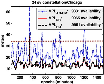
Figure 1. VPL with PD and RD implementations.
Figure 1 shows VPL values are very similar for both implementations. However there is a slight availability gain from using the PD implementation. This gain is due to the fact that the PD implementation allows reaching back in time to find a better reference geometry. However, the acceptable CT is limited by the rapid growth of differential SV clock and tropospheric delay errors. Reference times were searched up to one hour before the current epoch, but the smallest VPLPD was never found to be one using a reference epoch more than 3 minutes old. This can be seen in Figure 2, where the CT that gives the smallest VPLPD for each epoch is shown.

Figure 2. CT for smallest VPLPD at each epoch.
9. CONCLUSION
The use of Relative Receiver Autonomous Integrity Monitoring (RRAIM) for aircraft precision approach navigation was investigated in this paper. In the concept investigated, the responsibility for detecting Hazardously Misleading Information is divided between the RRAIM-equipped user and the navigation system provider, whose space and ground systems provide the basis for a GNSS Integrity Channel (GIC). The GIC performs ranging source integrity screening, generates corrections, and then broadcasts this information to users worldwide via a space based communication channel. During the correction processing and communication interval, there will be a latent period during which the user must rely on past GIC information. This latency can be a few seconds to several minutes, depending on the implementation. The user is continuously positioning in real time, and integrity against threats occurring during the latency period can be provided by RRAIM.
In this paper two versions of RRAIM were studied: a Range Domain (RD) and a Position Domain (PD) implementation. In both cases the user stores past carrier smoothed code and carrier phase measurements, and selects from those a reference epoch for which it has already received the GIC corrections. In both cases the user has three sets of measurements to use: the stored code measurements with corrections from the reference epoch (whose integrity is ensured by the GIC), a stored carrier phase measurement from the same reference epoch, and the current carrier phase measurement.
In the RD implementation the user creates a set of projected measurements by adding time-differential carrier phase measurements (current minus reference) to the reference GIC-corrected code measurements. The user position is obtained directly using these projected measurements. This implementation and corresponding covariance analysis is relatively straightforward. However, it requires use of only those ranging sources that are continuously available between the current and reference epochs.
The PD implementation generates an initial user position at the reference epoch using the corrected code measurements, and then adds to it a differential position vector, generated with the differential carrier phase measurements. The PD implementation allows for the use of all ranging sources available at the reference time to generate the initial position. The disadvantage is that the covariance analysis is significantly more complicated, and the corresponding bounding protection levels are more difficult to define. This is true because the carrier differential position error includes the effects of changes in user-SV lines of sight. These geometry changes introduce a correlation between the differential (current minus reference) carrier phase position error and the initial code-based reference position error. When latencies of several minutes are considered, these effects cannot be neglected, and have therefore been carefully analyzed and modelled in this paper.
The RRAIM detection function described in this paper is the same for both the RD and the PD implementations, as it needs only detect hazardous measurement errors during the latency period (because for the initial position integrity is provided by the GIC). When general error models for the corrected code measurement errors are considered, including potential unknown biases and Gaussian errors, the geometry change effects introduce a non centrality parameter in the fault free χ2 distribution of the RRAIM residual. This effect is carefully taken into account in this work.
In summary, this work provides the general formulas and derivations for positioning, fault detection, and protection level generation to meet a given set of integrity and continuity requirements. The mathematical justification of assumptions and models is provided, along with practical algorithms that pave the way toward real time implementation. An example of VPL results using the two algorithms was also provided.
The RRAIM architectures described in this paper have the advantage of not being excessively demanding on satellite constellation size, and they also allow the GIC segment to significantly relax requirements on time to alarm. They provide an improvement in worldwide navigation using methods that are straightforward enough to not pose serious obstacles in certification or installation on the user's end. However, the actual implementation of this architecture will depend on strategic non-technical decisions, like the future size of the constellations, the ability to install ground stations world-wide, and/or the willingness to use satellites not operated by the user's own country.
ACKNOWLEDGEMENTS
The technical contributions and suggestions provided by Frank van Graas, Young Lee, Todd Walter, Juan Blanch, and J. P. Fernow are greatly appreciated. The authors gratefully acknowledge the Federal Aviation Administration for supporting this research. However, the views expressed in this paper belong to the authors alone and do not necessarily represent the position of any other organization or person.
APPENDIX A
In equations (4) and (6) we introduced the concept of FDC, and its corresponding probability of occurrence. But for compactness of development in the main text, neither equation explicitly addresses the magnitude of the fault nor which particular satellite is faulted. For example, a more precise way of writing (6) is:
where p(f i*) is the probability density function of the fault magnitude f i* for satellite i. Assigning an equal budget of the FDC integrity risk allocation to each satellite in view, we can obtain an expression for the protection level PL fi assuming a fault f i* for any given SV i.:
Because the fault magnitude density function p(f i*) is not known, to be conservative, we must assume that p(f i*)=1 for all values of f i*, and find the magnitude of f i* and the satellite i for which PL fi is maximized.
APPENDIX B
The detailed error models for GEAS simulations can be found in [Reference Walter, Enge, Blanch and Pervan3] and [5]. Below we provide specific parameter values used to generate the numerical results in this paper.


