


INTRODUCTION
Age-depth models provide the critical temporal foundation for individual paleoenvironmental archives, and are essential for quantifying rates of change, making comparisons among proxy records, and hypothesizing drivers of environmental change. In this contribution to the QR Forum, we use a sample of recently-published age-depth models to comment on current practices in building and reporting radiocarbon-based age models. We address options for model building, sampling strategies, dating densities, and how best to report age models and associated data. To supplement the literature sample, we also present a case study of building age-depth models for a lake sediment core that has 22 AMS 14C ages as well as an independent varve chronology, which we use to assess model accuracy. We do not provide an exhaustive review of current practices, nor a comprehensive guide to building age-depth models. Instead, our intention is to cast light and prompt discussion on the building and reporting of 14C-based age models.
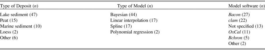
To take stock of current practices, we examined all papers published in 2018 and 2019 in Quaternary Research and Journal of Quaternary Science, and identified those that included 14C-based age-depth models that had not been previously published and did not rely on wiggle-matching to independent records for chronological control. We included all age-depth models regardless of sediment type or the temporal length of the record. We chose these two journals to concentrate our assessment of current practices on recently-produced models as opposed to previously-published models that are often included in review papers (e.g., Quaternary Science Reviews), without biasing the sample towards Holocene models (e.g., The Holocene) or those produced for lake sediments (e.g., Journal of Paleolimnology). Our compilation of models from Quaternary Research and Journal of Quaternary Science resulted in a sample of 80 age-depth models published in 62 papers (Supplementary Table 1), all with unique first authors. Almost half of the papers have a first author based in North America (45%); the other half are based in Europe (24%), China (13%) or elsewhere (18%). About half of the age models (59%) are fit to lake sediments, and the remaining are fit to peat (19%), marine sediment (13%), or other types of sediments (10%) such as loess, colluvium and floodplain deposits (Table 1). We take this to be a small but representative sample that provides sufficient grounds to comment on current practices in building and reporting 14C-based age-depth models. We did not observe a journal effect in any of our assessments i.e., current practices in papers published in the two journals appear to be more or less equivalent.
Table 1. Summary of 80 radiocarbon-based age-depth models published in Quaternary Research and Journal of Quaternary Science in 2018 and 2019.
CLASSICAL AND BAYESIAN AGE-DEPTH MODELS
In the last decade, the practice of modelling the relationship between depth and age has been advanced through wide availability of statistical code or programs for “classical” approaches such as clam (Blaauw, Reference Blaauw2010) and Bayesian modelling such as OxCal (Bronk Ramsey, Reference Bronk Ramsey2008), Bchron (Haslett and Parnell, Reference Haslett and Parnell2008) and Bacon (Blaauw and Christen, Reference Blaauw and Christen2011). An important advantage of using one of these programs is the 14C age calibration process that is dynamically included in the construction of models through repeated random sampling of the calibration distributions (Telford et al., Reference Telford, Heegaard and Birks2004a, Reference Telford, Heegaard and Birks2004b; Michczynski, Reference Michczynski2007; Blaauw, Reference Blaauw2010). Regardless of the type of model chosen, consideration of full calendar age probability distributions during model construction is a more robust approach than calibrating each 14C age in insolation (e.g., using CALIB; Stuiver and Reimer, Reference Stuiver and Reimer1993) and then building an age model on the single calibrated age estimates (e.g., the weighted average or median of the probability distribution). While most of the models in our literature sample took advantage of the built-in age calibration in one of these programs, 20% of the models were built on 14C ages that were reduced to single calibrated age points before model building. In some cases, these models might be reasonable approximations of the true age-depth relationship, but given that code and programs with built-in calibration processes are now readily available, this approach should be abandoned.
The simplest approach for constructing an age-depth model is to use linear interpolation between 14C ages. Linear interpolation assumes that ages are accurate and that accumulation rates between ages are linear. This was arguably the most commonly used approach for building chronologies 30 years ago (Webb and Webb, Reference Webb and Webb1988). In our literature sample, 21% of recently-published age models relied on simple linear interpolation, and many of these models were built in unspecified programs (Table 1). Linear interpolation models suffer from the problem that inferred changes in accumulation rate occur only, but exactly, at every dated depth (Bennett, Reference Bennett1994). This means that had 14C ages been obtained at different depths, changes in sedimentation rate would be located at different but equally-precise positions in the sequence. As pointed out by Bennett and Fuller (Reference Bennett and Fuller2002), “rates of sediment accumulation do not, in nature, change at the locations chosen for radiocarbon dates.”
In many cases, a smooth sedimentation rate is more realistic, at least in cases where sediment or peat type does not change abruptly. Thus, another approach is to use one of many classes of smooth functions: 21% of models in our literature sample used a smooth, cubic or monotonic spline, whereas only a few relied on polynomial regression (Table 1). These approaches use all of the dating information from the whole sediment sequence or core to model accumulation as a function of time. These models are now typically built in the clam package (Blaauw, Reference Blaauw2010) in R. In our literature sample, 28% of all models were built using clam (Table 1). Unfortunately, clam offers few diagnostics to help choose the best model. Nonetheless, citations of clam have substantially increased since it was first introduced (Yue Wang et al., Reference Wang, Goring and McGuire2019), with researchers using clam to implement various smooth functions as well as linear interpolation.
An alternative methodology for age-depth modelling is to use the Bayesian techniques available in OxCal (Bronk Ramsey, Reference Bronk Ramsey2008), Bchron (Haslett and Parnell, Reference Haslett and Parnell2008) and Bacon (Blaauw and Christen, Reference Blaauw and Christen2011). These Bayesian approaches enforce monotonicity of ages (positive accumulation rates) and incorporate assumptions about accumulation rates (e.g., Goring et al., Reference Goring, Williams, Blois, Jackson, Paciorek, Booth, Marlon, Blaauw and Christen2012) and/or how they vary, although in each program these are based on different depositional models with different parameters. The popularity of Bayesian techniques appears to be increasing. Yue Wang et al. (Reference Wang, Goring and McGuire2019) document a fairly consistent increase in citations of OxCal (Bronk Ramsey, Reference Bronk Ramsey2008) and Bacon (Blaauw and Christen, Reference Blaauw and Christen2011), although in many cases OxCal is used solely for 14C age calibration and not model building. Half of the models in our literature sample relied on a Bayesian approach, with most of these built using Bacon (34%), rather than OxCal (14%) or Bchron (6%). Like clam, there are few diagnostic tools in these programs to help choose the best model. With Bacon, it is also difficult to know when to change default values for accumulation rate priors and segment lengths, and the manual provides little guidance on setting model parameters. As a consequence, of the Bacon models in our literature sample that reported priors, most (73%) used the default values, regardless of whether the model was built for lake sediment, peat, or another type of sedimentary record.
Although Bayesian techniques use a different approach in the construction of age models, the ‘best-fit’ model can resemble simple linear interpolation e.g., when the mean age-depth model goes through each calibrated age range with changes in accumulation rate at dated depths. Resemblance to linear interpolation occurred in half (48%) of the Bacon models we examined (e.g., Yongbo Wang et al., Reference Wang, Zhang, Sun, Chang, Liu, Ni and Ning2019; McCulloch et al., Reference McCulloch, Mansilla, Morello, De Pol-Holz, San Román, Tisdall and Torres2019) and most if not all of the OxCal (e.g., Frodlová et al., Reference Frodlová, Hájková and Horsák2018) and Bchron (e.g., Schiferl et al., Reference Schiferl, Bush, Silman and Urrego2018) models. Trachsel and Telford (Reference Trachsel and Telford2017) observed that “although Bayesian age-depth modelling routines simulate changing accumulation rates, the mean accumulation rate (that is mostly used by scientists) is fairly constant between two dated levels, and therefore, the age-depth model is a straight line between two dated levels.” Similarity to linear interpolation is not altogether surprising, especially for Bacon and Bchron, as they are based in part on modelling piece-wise linear accumulations. For example, Parnell et al. (Reference Parnell, Buck and Doan2011) explain that an important constraint in Bchron is that a change in sedimentation rate is assumed to occur at each dated depth, thus treating each age as accurate as is the case in linear interpolation. Consequently, in the absence of many ages, these Bayesian techniques can result in a ‘best-fit’ model that resembles linear interpolation, albeit with improvements in uncertainty estimation (Trachsel and Telford, Reference Trachsel and Telford2017; Blaauw et al., Reference Blaauw, Christen, Bennett and Reimer2018).
Assessing the accuracy of age models requires that the true age-depth relationship be known, which is rarely the case. Model comparisons and tests of model accuracy have generally relied on simulations e.g., using varve chronologies to produce a series of simulated 14C ages upon which various models are built and then compared to the known varve chronology (Telford et al., Reference Telford, Heegaard and Birks2004a). Using this approach with three independent varve chronologies, Trachsel and Telford (Reference Trachsel and Telford2017) showed that Bayesian models built in Bacon, OxCal and Bchron as well as a smooth spline model from clam each produced a mean age model close to the true varve age; however, all models were challenged to produce reliable accumulation rates. In another simulation study, Wright et al. (Reference Wright, Edwards, van de Plassche, Blaauw, Parnell, van der Borg, de Jong, Roe, Selby and Black2017) concluded that no single modelling package (clam, OxCal, Bchron, and Bacon and its predecessor Bpeat) out-performed all others. Blaauw et al. (Reference Blaauw, Christen, Bennett and Reimer2018) compared the accuracy of linear interpolation, smooth spline, Bacon and Bchron models to a varve chronology as well as simulated hypothetical sequences, varying the dating density to further assess model accuracy. Their simulations demonstrate that, at low dating densities (<1 date per millennium, dpm), most models fail to accurately reproduce known age-depth relationships. The accuracy of all models improved as dating density increased, but this was especially the case with Bacon-produced models, which were more consistently accurate in their simulations, although even these models were offset from true age at high dating densities.
A significant difference between Bayesian and classical models, especially linear interpolation, lies in the estimation of age uncertainties. In Bayesian models, age uncertainties tend to increase between chronological control points e.g., with distance from 14C ages (Parnell et al., Reference Parnell, Buck and Doan2011; Trachsel and Telford, Reference Trachsel and Telford2017; Blaauw et al., Reference Blaauw, Christen, Bennett and Reimer2018). In contrast, models built with methods such as polynomial regression and smooth splines typically have uncertainties that are relatively constant between dated levels, and uncertainties in linear interpolation models may even decrease between ages (Bennett, Reference Bennett1994; Trachsel and Telford, Reference Trachsel and Telford2017; Törőcsik et al., Reference Törőcsik, Gulyás, Molnár, Tapody, Sümegi, Szilágyi and Molnar2018). Trachsel and Telford (Reference Trachsel and Telford2017) suggest that smooth splines in clam usually underestimate age uncertainties and that Bayesian approaches generally provide better error estimation, although these can be too large in Bchron and too large or too small in Bacon and OxCal, depending on how modelling routines are parameterized. Similarly, Blaauw et al. (Reference Blaauw, Christen, Bennett and Reimer2018) argue that linear interpolation and smooth splines produce age uncertainties that are too narrow and that the wider uncertainties in Bacon and Bchron are more realistic. However, age uncertainties produced by the various programs are different types of uncertainties, making their direct comparison less meaningful. The Bayesian programs provide age uncertainties for single predicted ages for a given depth (i.e., prediction intervals), whereas clam returns confidence intervals that are uncertainties on the mean predicted age for a given depth (Trachsel and Telford, Reference Trachsel and Telford2017). This is a subtle but important difference that likely helps to explain why uncertainties in clam are almost always lower than in the Bayesian models; predicting a single age for a given depth is inherently more uncertain than predicting its mean age.
Age uncertainties are important for assessing the synchronicity of paleoenvironmental changes among records and/or sites, and identifying the drivers of such changes. There are, however, few examples in the literature of studies that explicitly integrate age model uncertainties into paleoenvironmental reconstructions (e.g., Charman et al., Reference Charman, Barber, Blaauw, Langdon, Mauquoy, Daley, Hughes and Karofeld2009; Blaauw et al., Reference Blaauw, Wohlfarth, Christen, Ampel, Veres, Hughen, Preusser and Svensson2010; Chevalier and Chase, Reference Chevalier and Chase2015). In the vast majority of studies, researchers are interested in the ‘best fit’ or mean modelled age for individual depths (i.e., point estimates) and pay little attention to age model uncertainties or precision. Although 84% of the papers in our literature sample showed uncertainties on a plot of the age model, none made explicit use of the uncertainties in their paleoenvironmental reconstructions. Weller et al. (Reference Weller, de Porras, Maldonado, Méndez and Stern2019) was the only paper to use uncertainty estimates in a tangible way i.e., in the assignment of ages to poorly-dated tephras. Consideration of age model uncertainties will need to be incorporated into paleoenvironmental reconstructions for the advances provided by Bayesian age models to be fully realized.
DATING DENSITIES AND SAMPLING STRATEGIES
The degree of chronological control in an age-depth model acts as an important constraint on the research questions that can be answered in any given study. One basic measure of chronological control is dating density i.e., the number of ages per time interval. Blaauw et al. (Reference Blaauw, Christen, Bennett and Reimer2018) note that, on average, late Quaternary sites in the Neotoma database (Williams et al., Reference Williams, Grimm, Blois, Charles, Davis, Goring and Graham2018) have the equivalent of one 14C age every 1400 yr (or 0.72 dates per millennium) and that only 14% of sites have >2 dpm. To estimate dating densities in our sample of 80 recently-published age-depth models, we included 14C ages as well as other chronological control points such as known tephras and ages that had been assigned to 0 cm, typically the year of sediment core collection. Only 20% of the models in our literature sample had >2 dpm; with only one exception, these well-dated records span 6000 years or less. The mean across all 80 models was 1.4 dpm (median = 1.0 dpm). Dating densities were slightly higher in models spanning the last 15,000 years or less (mean = 1.8 dpm, median = 1.4 dpm; n = 52). On average, this indicates an age every 600 to 700 yr, which comes close to Blaauw et al.'s (Reference Blaauw, Christen, Bennett and Reimer2018) recommendation of obtaining a minimum of 2 dpm. Taken at face value, this suggests a respectable amount of chronological control in recently-published models, particularly in light of the constraints imposed by research funding. The accuracy of age models should generally increase with higher dating densities (Telford et al., Reference Telford, Heegaard and Birks2004a; Trachsel and Telford, Reference Trachsel and Telford2017; Blaauw et al., Reference Blaauw, Christen, Bennett and Reimer2018), provided the ages themselves are reasonably accurate. Of course, the maximum number of dates, given funding constraints, should be obtained. However, using the mean number of ages per millennium to assess model quality ignores what we refer to below as the ‘age spacing problem'.
Many of the age-depth models in our literature sample suffer from long temporal gaps between ages e.g., gaps of >3000 yr between ages in full Holocene records, gaps of >1000 yr in records spanning 3000 yr, etc. Of the 80 models, two-thirds (64%) suffered from this ‘age spacing problem', leaving these records with poor chronological control in portions of the record. Some particularly-poorly constrained sequences had two or three long gaps between ages. Others had a number of ages within a short time interval, which reduces the quality of the overall age-depth model compared to having the same number of ages spread over longer intervals. Thus, the issue is not solely whether sufficient ages are being used to build age models but also how closely spaced the ages are in time. Of course, the length of tolerable gaps will depend on the research question(s). Nonetheless, we recommend, based on common sense, that researchers avoid long temporal gaps between dated levels e.g., gaps of more than 20% of the total length of the record. We acknowledge that in some cases, especially in regions such as the Arctic, long temporal gaps may be unavoidable, if there is insufficient carbon for dating in long sections of a sediment sequence. Of course, additional ages should be obtained for sequences with substantial changes in accumulation rates and those subjected to high-resolution proxy analyses.
Building a robust age model begins with choices on what to date and where along a sequence to obtain ages. Attention must be paid to deciding how many ages to obtain and what material to date (e.g., MacDonald et al., Reference MacDonald, Beukens and Kieser1991; Björck and Wohlfarth, Reference Björck, Wohlfarth, Last and Smol2001; Oswald et al., Reference Oswald, Anderson, Brown, Brubaker, Hu, Lozhkin, Tinner and Kaltenrieder2005; Walker et al., Reference Walker, Davidson, Lange and Wren2007; Grimm et al., Reference Grimm, Maher and Nelson2009; Piotrowska et al., Reference Piotrowska, Blaauw, Mauquoy and Chambers2011). When the number of ages is constrained by the availability of funds, the best strategy involves several iterations of dating i.e., obtaining a first batch of ages spread along the length of the sequence, including one near or at the base, followed by second and/or third batches in which additional depths are chosen strategically so that ages are more or less evenly spread in time and changes in sediment type or accumulation are considered (PALE Steering Committee, 1993; Bennett, Reference Bennett1994; Piotrowska et al., Reference Piotrowska, Blaauw, Mauquoy and Chambers2011; Blaauw et al., Reference Blaauw, Christen, Bennett and Reimer2018). Large changes in accumulation rates are usually only discovered after dating; thus, dating in batches helps to produce a better model. To assess the extent to which models in our literature sample were built with ages obtained in batches, we examined the lab reference numbers reported for each 14C age in every paper. Because analytical labs generally number 14C ages in the order in which they are produced, models built on 14C ages obtained in a single batch should have lab numbers that are in numerical order (e.g., the UOC ages in Table 2), while 14C ages with notably different lab numbers or from different labs indicate iterations of dating. For the chronologies in our literature sample that reported lab numbers (26% of papers did not report lab codes), only 21% had lab numbers that were in order, suggesting that most researchers are indeed using several iterations of dating to refine their chronologies. However, we found that two-thirds (69%) of the age models with lab numbers in numerical order had the ‘age spacing problem’ described above. Two or more iterations of dating should help avoid long temporal gaps between ages.
Table 2. AMS radiocarbon ages from Lac Noir, southwestern Québec, Canada from Neil and Gajewski (Reference Neil and Gajewski2018). All 14C ages are on plant remains including leaf fragments, seeds and needles.
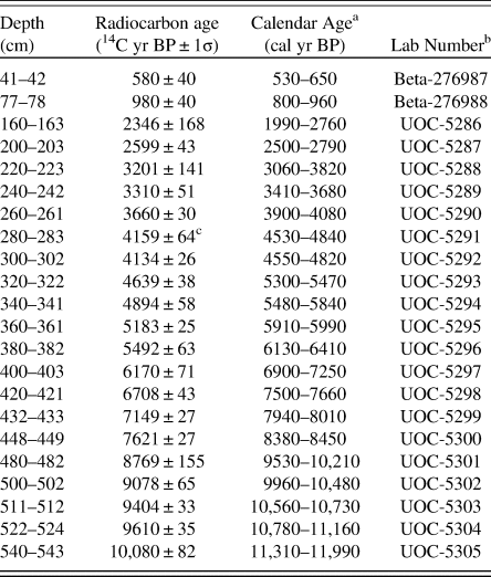
a 2σ calendar age range rounded to the nearest 10 yr; from CALIB 7.1 based on IntCal13 (Reimer et al., Reference Reimer, Bard, Bayliss, Beck, Blackwell, Bronk Ramsey and Buck2013)
b Beta = Beta Analytic Inc.; UOC = University of Ottawa A.E. Lalonde AMS Laboratory
c Excluded from the linear interpolation models only
As a general rule, extrapolating an age-depth model beyond the dated range of a sediment sequence should be avoided, as it assumes that the relationship between depth and time holds for sediments lacking chronological control. Extrapolation should not be used across changes in sediment or peat type. Excessive extrapolation, which we defined as 1000 years or more beyond the oldest 14C age, was used in only 14% of the models we examined; however, in a few cases, the age model was extrapolated by several thousand years. In cases where basal sediments lack chronological control, we recommend that proxy data below the lowest age be plotted without a timescale.
REPORTING AGE-DEPTH MODELS
All 14C ages and associated methods need to be described in adequate detail if others are to successfully reproduce an age-depth model, update the model as new calibration datasets and modelling techniques are developed, or use the data in large-scale synthesis efforts. Of course, meta-data on 14C ages and the steps taken to build a chronology are also necessary for assessing the quality of age models and the paleoenvironmental inferences that rely on them.
We were surprised to find that one-third (34%) of the papers we examined failed to report one or more of the following: whether the ages were based on AMS or radiometric 14C dating, what material was dated, the name of the lab that performed the dating, and/or the lab reference numbers for each 14C age. In addition, nearly one-quarter (23%) of papers did not report which 14C calibration dataset was used. Of the 34 papers that reported 14C ages on bulk sediment or peat, 74% failed to report sample thickness. Sample thickness is important information for reproducing or updating an age model, as it is the midpoints of the depth ranges that should be used in age-depth modelling. A number of papers also failed to specify important parameters used in model construction. For example, 54% of papers that used Bacon did not report the priors that are essential to this Bayesian technique. The upper panels of a default Bacon age-depth plot include the priors as well as information about model iterations; however, these panels are often omitted from publications. We suspect in most cases where the priors were not reported that default values were used, as that is by far the most common approach. Information about priors along with which version of Bacon should always be reported, because the default priors have changed between versions. We also encourage inclusion of δ13C values for each 14C age but only when measured independently through isotope-ratio mass spectrometry (IRMS). These values can potentially provide information about the material being dated and/or the environmental conditions the sample is derived from.
Assigning an age to the surface or top of the sequence is now common practice. Almost two-thirds of the papers in our literature sample used an assigned top age in their age model e.g., the year of sediment core collection for 0 cm. However, the majority of papers (86%) that assigned a top age failed to report the details of the age. In some cases, it was apparent in the plot of the model that a top age was used to constrain the chronology, but this constraint was not stated in any way in the text. In other cases, the paper stated that a top age was used in the model, but the specific age and its error were not reported. In fact, the year of sediment collection, whether it was used in the age model or not, was not reported in 40% of papers in our literature sample. When a top age is used as a control point in an age-depth model, its depth and assigned age and error must be reported.
Given the central role of age models, both a table of 14C ages and a plot of the model should be included. Plots of age-depth models should include both the ‘best-fit’ model used for proxy data as well as age uncertainty estimates. Building an age-depth model is a statistical exercise (i.e., age = ƒ(depth) + error) and as such, depth belongs on the x-axis, as it is the known variable from which age is predicted (Bennett, Reference Bennett1994). However, in our sample of recently-published models, most placed depth on the y-axis, which implies, according to statistical convention, that depth was predicted from age.
Rejection of 14C ages was surprisingly common in the papers we examined. In 33% of cases, one or more 14C age was rejected before model building, primarily because of age reversals. In many cases, rejected ages are not included in the plot of the age-depth model. We recommend including rejected ages not only in the table of ages but also in the age model plot, as this aids assessment of the context, validity and implications of age rejections. All of the model-building programs discussed above include some sort of ‘outlier’ argument or command that can be used to plot a rejected age while still excluding it from the model.
LAC NOIR: A CASE STUDY IN AGE-DEPTH MODELLING
Simulation studies such as those by Trachsel and Telford (Reference Trachsel and Telford2017) and Blaauw et al. (Reference Blaauw, Christen, Bennett and Reimer2018) provide much-needed insight into the performance of age-depth models. However, as pointed out by Telford et al. (Reference Telford, Heegaard and Birks2004a), these simulations are often conducted under conditions that are notably different from building age models with real datasets: the simulated ages are accurate, precise and often equally-spaced, and there are no concerns about contamination, reservoir effects, hiatuses, or extreme changes in accumulation rates.
Here, we compare a series of age-depth models built for a well-dated lake sediment core that has an independent varve chronology. This provides an opportunity to assess the performance and accuracy of models built on real ages, as opposed to simulations. The sediment core is from Lac Noir (45°46.53'N, 75°8.10′W) in southwestern Québec, Canada (Neil and Gajewski, Reference Neil and Gajewski2018), is 5.43 m long, and has 22 AMS 14C ages (Table 2), resulting in a dating density of 2 dpm. The sediments are continuously laminated to a depth of 5.24 m with varves spanning the last 11,160 cal yr. We treated the varve chronology as true and accurate, although replicate varve counts indicate counting imprecision of 1.5 to 6.7% depending on the core section (Neil and Gajewski, Reference Neil and Gajewski2018). We fit the three most common types of models encountered in our literature sample: a Bayesian model using the default priors in Bacon (vers. 2.3.9.1), and linear interpolation and smooth spline models using clam (vers. 2.3.2). We also fit a 2nd-order polynomial, as it represents an end-member of models to choose from and polynomials were commonly used in older studies. For linear interpolation, we excluded the 14C age at 280 cm (Table 2) prior to model construction. The age is from a ‘flat’ portion of the calibration curve and causes a minor age reversal. Thus, excluding this age was necessary for linear interpolation but unnecessary when fitting the other models. In a second iteration, we built all four models using only every second 14C age to assess their performance at a dating density (i.e., 1 dpm) that is typical of many published studies. In all cases, we used an age of −62 ± 2 cal yr BP for 0 cm, based on the year of core collection (2012). We focus on the ‘best-fit’ models (Figs. 1 and 2) and their associated sediment accumulation rates (Fig. 3), as these have important implications for estimating proxy accumulation rates, and place less emphasis on estimated age uncertainties as these are not directly comparable between Bacon and clam.

Figure 1. Age-depth models fit to the AMS radiocarbon ages from Lac Noir (Table 2) and an age of −62 ± 2 cal yr BP for 0 cm. Blue symbols show the 22 calibrated 14C ages and their probability distributions as calibrated by Bacon vers. 2.3.9.1 and clam vers. 2.3.2. All clam models were run with 10,000 iterations. (A) Mean age-depth model from Bacon (blue) built using default priors of 20 yr cm-1 and 1.5 for mean deposition time and shape, respectively, with its 95% prediction intervals in grey. Linear interpolation model (red) from clam without confidence intervals and the varve chronology (dashed black) are also shown. Prior to model construction, the 14C age at 280 cm was excluded from the linear interpolation model only. The linear interpolation model (red) is mostly obscured by the ‘best-fit’ Bacon model (blue) because of their similarity. (B) Smooth spline model (blue) and its 95% confidence intervals in grey, built with default smoothing of 0.3 in clam. A 2nd-order polynomial model (orange) from clam without confidence intervals and the varve chronology (dashed black) are also shown.


Figure 3. Accumulation rates for the age-depth models in Figure 1. In all panels, rates based on varve thickness measurements are shown as open grey symbols and vertical dashed lines show the median of the probability distribution of each calibrated 14C age. (A) Loess curve (black; loess span = 0.2) fit to accumulation rates based on varve thickness, and accumulation rates from the 2nd-order polynomial model (orange) in Fig. 1B. (B) Accumulation rates based on the default ‘best-fit’ Bacon model (blue) in Fig. 1A showing its 5-cm linear segments, linear interpolation (black) in Fig. 1A, and the clam-based smooth spline (red) with default smoothing of 0.3 in Fig. 1B. (C) The same as panel B, except models are based on only every second 14C age in Table 2 to mimic a more typical dating density.
The mean age-depth model from Bacon goes through each calibrated age range with age uncertainties that are mostly between 275 and 500 yr (Figs. 1A and 2A). Linear interpolation behaves similarly (Fig. 1A), but its uncertainties (not shown) are mostly smaller (150 to 350 yr). The median differences between the Bacon and linear interpolation models compared to the varve chronology are 223 and 228 yr, respectively (Fig. 2A). It is difficult to distinguish the ‘best-fit’ Bacon and linear interpolation models, except in the few sections of the core where they differ (Fig. 1A). However, differences are readily apparent in their estimated accumulation rates (Fig. 3B), which show the linear segments fit in each case i.e., between pairs of 14C ages in linear interpolation and for each of the 5-cm segments in Bacon. The mean model from Bacon introduces high frequency changes in accumulation rates that vary in amplitude, whereas for linear interpolation, rate changes are mostly high in amplitude with their frequency more tightly controlled by the position of the 14C ages. At the lower dating density, the two models (Fig. 2B) and their accumulation rates (Fig. 3C) are almost indistinguishable, although Bacon retains high frequency changes in rates linked to segment length. This underscores the importance of high dating densities when fitting models in Bacon (Blaauw et al., Reference Blaauw, Christen, Bennett and Reimer2018). At the lower dating density, the Lac Noir accumulation rates of the mean model from Bacon are not substantially different from simple linear interpolation.
The smooth spline (Figs. 1B and 2A) fit in clam also goes through each calibrated age range, but its age uncertainties are generally smaller than the Bacon model. Uncertainties are generally between 130 and 260 yr but are up to 600 yr in the late Holocene where Bacon also returns large uncertainties. The median difference between the smooth spline and the varve chronology is 231 yr, which is similar to Bacon and linear interpolation, and down-core changes in accuracy are also similar to Bacon (Fig. 2A). Accumulation rates for the smooth spline generally increase and decrease in concert with those of Bacon (Fig. 3B), although rate changes are sometimes higher or lower in amplitude. At the lower dating density, changes in accumulation rates for the smooth spline are, of course, smoother but are also generally similar to Bacon and linear interpolation over the long-term (Fig. 3C).
As expected, the 2nd-order polynomial produces an even smoother age-depth model (Fig. 1B), uncertainties are at their lowest and have a relatively constant width (~100 yr for most depths), and accumulation rates are also relatively constant for much of the sediment core (Fig. 3A). The median difference compared to the varve chronology is 129 yr, which is substantially lower than the other three models (Fig. 2A). At the lower dating density, the polynomial model and its accumulation rates are essentially unchanged, although this is not surprising for a low-degree polynomial.
Comparison to the Lac Noir varve chronology shows that all models are accurate in some sections but over- or underestimate age in others (Figs. 1 and 2). In addition, linear interpolation, Bacon and the smooth spline over-estimate variability in accumulation rates compared to those based on varve thickness, and changes are frequently out of phase (Fig. 3B). Although most of the calibrated age ranges at Lac Noir overlap the varve chronology (Fig. 1), 14C ages between 450 and 360 cm depth (~8400 and 6000 cal yr BP) are generally younger than the corresponding varve age and those above 220 cm depth (<3000 cal yr BP) are generally older. These systematic offsets may be related to changes in plant communities, lake chemistry and/or other environmental conditions. Regardless, these age offsets highlight another important consideration in the construction of age-depth models: each 14C age is merely a sample of n = 1 of the total population of ages for any given depth. Thus, it should not be surprising when 14C ages, and models based on them, deviate from true age. In the case of Lac Noir, none of the modelled age uncertainties fully encapsulate the varve chronology. The default Bacon model is most successful in this regard, but even in this case, the age uncertainties encompass the varve chronology for only 40% of the record's length (Figs. 1A and 2A).
Given that all of the models over and under-estimate age in similar sections of the record, there is no obvious choice for the ‘best model'. In general, the smooth spline and polynomial are more effective at mimicking the smoothness of the varve chronology over the long term. If proxies such as loss-on-ignition or magnetic susceptibility are also smooth (as at Lac Noir; Neil and Gajewski, Reference Neil and Gajewski2018), then a smooth model may be a reasonable choice. Among all four models, the polynomial has the lowest deviations, on average, from the varve chronology (Fig. 2A), but it clearly underestimates variability in accumulation rates, especially in the past ~4000 years (Fig. 3A). The ‘best-fit’ Bacon model is an improvement over simple linear interpolation and is fairly similar to the smooth spline (Fig. 2A), although Bacon appears to overestimate variability in accumulation rates (Fig. 3B), as also shown by Trachsel and Telford (Reference Trachsel and Telford2017). Increasing the segment length in Bacon from the default 5 cm to match the median (20 cm) or mean (25 cm) distance between 14C ages further increases the resemblance between Bacon and linear interpolation, although changes in the Bacon-produced accumulation rates sometimes lead or lag the position of the 14C ages. Wright et al. (Reference Wright, Edwards, van de Plassche, Blaauw, Parnell, van der Borg, de Jong, Roe, Selby and Black2017) found similar phase offsets with Bacon-produced models.
Interestingly, the modelled ages and accumulation rates of all four models are as or more similar to the varve chronology when fit using only half of the 22 14C ages (Figs. 2B and 3C). At the lower dating density (Fig. 2B), the median difference compared to the varve chronology is lowest for the polynomial (110 yr) and highest for the Bacon model (200 yr). For Lac Noir, a higher dating density does not result in a more accurate age model (cf. Blaauw et al., Reference Blaauw, Christen, Bennett and Reimer2018). The overall pattern of sediment accumulation at Lac Noir is smooth and broadly linear, and fewer dates result in less scatter, so it is not surprising that models built using a lower dating density have similar or better accuracy. However, this is not likely to be the case for records with more substantial changes in sedimentation rates. Simulation studies have shown that low dating densities typically decrease model accuracy (Telford et al., Reference Telford, Heegaard and Birks2004a; Trachsel and Telford, Reference Trachsel and Telford2017; Blaauw et al., Reference Blaauw, Christen, Bennett and Reimer2018).
In light of our model comparisons using the Lac Noir record as well as the simulation studies of others (Telford et al., Reference Telford, Heegaard and Birks2004a; Trachsel and Telford, Reference Trachsel and Telford2017; Wright et al., Reference Wright, Edwards, van de Plassche, Blaauw, Parnell, van der Borg, de Jong, Roe, Selby and Black2017), we cannot support the blanket recommendation by Blaauw et al. (Reference Blaauw, Christen, Bennett and Reimer2018) that Bayesian models be used in building chronologies, to the apparent exclusion of other types of models. Much depends on dating densities, age scatter, outliers, and down-core changes in sediment type and accumulation rates. Instead, as suggested by Blockley et al. (Reference Blockley, Blaauw, Ramsey and van der Plicht2007), an array of models could be entertained along with assessment of how well each approximates the chronological data and satisfies other information such as changes in sediment type or other properties. This approach should clarify what effects, if any, the routines and assumptions of each modelling approach have on the resulting age model and accumulation rates, and may suggest, at least informally, the confidence that can be attached to conclusions based on associated proxy data. In addition, modelled accumulation rates should not be blindly imposed on proxy data e.g., in calculating pollen or carbon accumulation rates. Attention should be paid to how model-driven changes in accumulation rates might affect paleoenvironmental inferences from proxy accumulation rates. To be clear, we are not suggesting that researchers fit all possible models and choose the one deemed most desirable. Rather, we are arguing against the other extreme of relying solely on a single modelling technique for all scenarios. Consideration should be given to whether the chosen model, Bayesian or not, is sensible given other evidence on the age-depth relationship and the history of sediment or peat accumulation.
LOOKING FORWARD
Our recommendations on best practices for building and reporting age-depth models are not new nor are they exhaustive, but they bear repeating. When building an age-depth model, 14C ages should not be reduced to single calibrated age estimates before model construction, as there are now a number of modelling options with built-in age calibration. To the extent possible, researchers should avoid long temporal gaps between ages. Obtaining 14C ages in batches is part of an effective strategy for avoiding long temporal gaps. High density dating is particularly important for sequences with substantial changes in accumulation rates and those subjected to high-resolution proxy analyses. Extrapolation beyond chronological control points is rarely justified. Our review of recent studies illustrates that better reporting of 14C ages, model-building methods, age-depth models and associated meta-data is needed. All information needed to evaluate, reproduce and update an age model should accompany every published model. This includes reporting the material that was dated, sample thicknesses, radiocarbon lab names and reference codes, and calibration datasets. Details on assigned surface ages, rejected ages and all modelling parameters including Bayesian priors should also be reported.
Varve chronologies such as Lac Noir and others used in simulation studies (Telford et al., Reference Telford, Heegaard and Birks2004a; Trachsel and Telford, Reference Trachsel and Telford2017; Blaauw et al., Reference Blaauw, Christen, Bennett and Reimer2018) are useful in assessing model accuracy, but sedimentation in varved records tends to be fairly smooth and broadly linear. In contrast, two-thirds of the age-depth models in our literature sample had sigmoidal, concave or convex shapes. Future assessments of model performance should attempt to address these more complicated but routinely-encountered age-depth relationships. In addition, user-friendly code for comparing models produced by different programs and more diagnostic tools for choosing the ‘best model’ would help advance efforts to identify robust age models. More work is needed to determine best practices for incorporating age model uncertainties into paleoenvironmental reconstructions. It would be helpful if an option for prediction intervals were added to clam, where this is feasible (e.g., splines, polynomials), as it is the most widely used program for classical age-depth modelling. This would facilitate comparison of model uncertainties among classical and Bayesian techniques, as the uncertainties that are currently provided are not directly comparable in a statistical sense. Approaches for integrating depth uncertainties (e.g., sample thicknesses) into age-depth models and for combining 14C and 210Pb ages in a single age model also warrant further investigation.
The case study at Lac Noir highlights the offsets between 14C ages and true age that may very well occur in many late Quaternary records. Obtaining high-precision AMS 14C ages on tiny discrete samples, in lieu of low-precision radiometric ages on bulk sediments, is now common practice. It is difficult to know if this approach might be increasing the likelihood that any given 14C age is offset from true age (Oswald et al., Reference Oswald, Anderson, Brown, Brubaker, Hu, Lozhkin, Tinner and Kaltenrieder2005; Walker et al., Reference Walker, Davidson, Lange and Wren2007). Regardless, these potential offsets are important to bear in mind. Age-depth model accuracy is ultimately controlled by the accuracy of the ages themselves.
ACKNOWLEDGMENTS
We thank the Senior Editors of Quaternary Research for the opportunity to contribute to the QR Forum, Mathias Trachsel for sharing information on age-depth model uncertainties, and Derek Booth, Maarten Blaauw and two anonymous reviewers for helpful feedback. Both authors are supported by research grants from the Natural Sciences and Engineering Research Council of Canada.
SUPPLEMENTARY MATERIAL
The supplementary material for this article can be found at https://doi.org/10.1017/qua.2020.47


