


1. Introduction
Fluid encapsulation is the process of entrapping one substance within another. Typical functions of encapsulation are to isolate an aggressive component from the environment and/or deliver one component it to a particular receptor (Loscertales et al. Reference Loscertales, Barrero, Guerrero, Cortijo, Marquez and Ganan-Calvo2002). This could be beneficial in processes involving transportation, coating, site-specific drug delivery, medical imaging as well as food, cosmetic and pharmaceutical product manufacturing (Gref et al. Reference Gref, Minamitake, Peracchia, Trubetskoy, Torchilin and Langer1994; Cohen et al. Reference Cohen, Li, Hougland, Mrksich and Nagel2001; Hillery, Lloyd & Swarbrick Reference Hillery, Lloyd and Swarbrick2001; Zuidam & Nedovic Reference Zuidam and Nedovic2010). Various techniques of encapsulation are proposed in the literature, e.g. Lister (Reference Lister1989), Ganan-Calvo (Reference Ganan-Calvo1998), Cohen et al. (Reference Cohen, Li, Hougland, Mrksich and Nagel2001), Loscertales et al. (Reference Loscertales, Barrero, Guerrero, Cortijo, Marquez and Ganan-Calvo2002), Jaworek (Reference Jaworek2008), Zhao et al. (Reference Zhao, Shum, Adams, Sun, Holtze, Gu and Weitz2011) and Windbergs et al. (Reference Windbergs, Zhao, Heyman and Weitz2013), but it is not our intention to review these here. A common feature of many current techniques is that they are limited to droplet sizes governed by capillary forces, i.e. short length scales. Instead here we propose a method of encapsulation focused at macro-scale droplets, independent of capillary forces.
Yield stress (viscoplastic) fluids have the property that they do not deform unless a given yield stress (
 $\hat{{\it\tau}}_{Y}$
) is exceeded. If the deviatoric stress is below the yield stress, the fluid acts like a rigid solid, resisting deformation. While in some flows this leads to unwanted features, e.g. Roustaei, Gosselin & Frigaard (Reference Roustaei, Gosselin and Frigaard2014), in other cases yield stress behaviour can be exploited in order to produce novel and beneficial flow features. One example of such flows, that we generalize here, is termed viscoplastically lubricated (VPL) flow, in which a yield stress fluid is used to stabilize the interface in a multi-layer flow; see Frigaard (Reference Frigaard2001), Moyers-Gonzalez, Frigaard & Nouar (Reference Moyers-Gonzalez, Frigaard and Nouar2004), Huen, Frigaard & Martinez (Reference Huen, Frigaard and Martinez2007), Hormozi, Wielage-Burchard & Frigaard (Reference Hormozi, Wielage-Burchard and Frigaard2011b
,Reference Hormozi, Wielage-Burchard and Frigaard
c
), Hormozi, Martinez & Frigaard (Reference Hormozi, Martinez and Frigaard2011a
) and Hormozi & Frigaard (Reference Hormozi and Frigaard2012). The main focus is pressure-driven duct flows in which a viscoplastic fluid adjacent to the wall lubricates a centrally positioned viscous fluid. By controlling the relative flow rate of the two fluids we can ensure that the yield stress is larger than the interfacial shear stress by a finite amount. This results in a finite unyielded region around the central fluid, preserving stability. Both linear and nonlinear stability results have been established, for Newtonian and non-Newtonian core fluids; see Frigaard (Reference Frigaard2001), Moyers-Gonzalez et al. (Reference Moyers-Gonzalez, Frigaard and Nouar2004), Moyers-Gonzalez, Frigaard & Nouar (Reference Moyers-Gonzalez, Frigaard and Nouar2010), Hormozi et al. (Reference Hormozi, Wielage-Burchard and Frigaard2011b
) and Hormozi & Frigaard (Reference Hormozi and Frigaard2012). Experimental studies have used viscous, shear-thinning and viscoelastic core fluids; see Huen et al. (Reference Huen, Frigaard and Martinez2007) and Hormozi et al. (Reference Hormozi, Wielage-Burchard and Frigaard2011c
).
$\hat{{\it\tau}}_{Y}$
) is exceeded. If the deviatoric stress is below the yield stress, the fluid acts like a rigid solid, resisting deformation. While in some flows this leads to unwanted features, e.g. Roustaei, Gosselin & Frigaard (Reference Roustaei, Gosselin and Frigaard2014), in other cases yield stress behaviour can be exploited in order to produce novel and beneficial flow features. One example of such flows, that we generalize here, is termed viscoplastically lubricated (VPL) flow, in which a yield stress fluid is used to stabilize the interface in a multi-layer flow; see Frigaard (Reference Frigaard2001), Moyers-Gonzalez, Frigaard & Nouar (Reference Moyers-Gonzalez, Frigaard and Nouar2004), Huen, Frigaard & Martinez (Reference Huen, Frigaard and Martinez2007), Hormozi, Wielage-Burchard & Frigaard (Reference Hormozi, Wielage-Burchard and Frigaard2011b
,Reference Hormozi, Wielage-Burchard and Frigaard
c
), Hormozi, Martinez & Frigaard (Reference Hormozi, Martinez and Frigaard2011a
) and Hormozi & Frigaard (Reference Hormozi and Frigaard2012). The main focus is pressure-driven duct flows in which a viscoplastic fluid adjacent to the wall lubricates a centrally positioned viscous fluid. By controlling the relative flow rate of the two fluids we can ensure that the yield stress is larger than the interfacial shear stress by a finite amount. This results in a finite unyielded region around the central fluid, preserving stability. Both linear and nonlinear stability results have been established, for Newtonian and non-Newtonian core fluids; see Frigaard (Reference Frigaard2001), Moyers-Gonzalez et al. (Reference Moyers-Gonzalez, Frigaard and Nouar2004), Moyers-Gonzalez, Frigaard & Nouar (Reference Moyers-Gonzalez, Frigaard and Nouar2010), Hormozi et al. (Reference Hormozi, Wielage-Burchard and Frigaard2011b
) and Hormozi & Frigaard (Reference Hormozi and Frigaard2012). Experimental studies have used viscous, shear-thinning and viscoelastic core fluids; see Huen et al. (Reference Huen, Frigaard and Martinez2007) and Hormozi et al. (Reference Hormozi, Wielage-Burchard and Frigaard2011c
).
The idea of encapsulation stems from these studies. We have looked to extend the VPL concept in different ways. For example, recently in Hormozi, Dunbrack & Frigaard (Reference Hormozi, Dunbrack and Frigaard2014) we have introduced periodic perturbations to the flow rates of initially stable VPL flows, resulting in stable patterned interfaces. In Hormozi et al. (Reference Hormozi, Wielage-Burchard and Frigaard2011b ) we have experimented numerically with different injection novel configurations in order to advect encapsulated ‘letters’ and ‘write’ in the flow. In this paper we expand this idea by considering the encapsulation of a regularly spaced stream of droplets evenly spaced within the plug region of a yield stress fluid flowing along a uniform duct. The main focus is to determine the size of droplets that can be encapsulated in this way, without yielding the encapsulating plug, for both plane channel and pipe configurations. Of course if instead of droplets, neutrally buoyant solid particles are transported, the particles are indistinguishable from the plug and exert no stress. On the other hand, transported droplets perturb the stress field in the encapsulating plug, ultimately breaking the plug for large droplets.
In the absence of fluid motions there are many studies of settling (or rise) in stationary yield stress fluid whereby the yield stress holds a particle (droplet or bubble) stationary until a certain critical buoyancy stress is exceeded. Thus, particles and bubbles below a certain size are held in suspension. Critical yield numbers are known for many symmetric particle geometries, e.g. spheres, cylinders, ellipsoids, and can be computed with care; see Beris, Tsamopoulos & Armstrong (Reference Beris, Tsamopoulos and Armstrong1985), Roquet & Saramito (Reference Roquet and Saramito2003), Tokpavi, Magnin & Jay (Reference Tokpavi, Magnin and Jay2008) and Putz & Frigaard (Reference Putz and Frigaard2010). There are similar studies that address the onset of bubble propagation; see Dubash & Frigaard (Reference Dubash and Frigaard2004, Reference Dubash and Frigaard2005), Tsamopoulos et al. (Reference Tsamopoulos, Dimakopoulos, Chatzidai, Karapetsas and Pavlidis2008) and Dimakopoulos, Pavlidis & Tsamopoulos (Reference Dimakopoulos, Pavlidis and Tsamopoulos2013). In both cases the yield stress fluid yields locally to the particle (bubble) and in the Stokes regime propagates slowly with yielded fluid being displaced from in front of the particle (bubble) to behind. There are many interesting studies focusing on moving particles and droplets, determining drag coefficients etc., e.g. Beris et al. (Reference Beris, Tsamopoulos and Armstrong1985), Beaulne & Mitsoulis (Reference Beaulne and Mitsoulis1997), Blackery & Mitsoulis (Reference Blackery and Mitsoulis1997), Liu, Muller & Denn (Reference Liu, Muller and Denn2002), De Besses, Magnin & Jay (Reference De Besses, Magnin and Jay2003), Mitsoulis (Reference Mitsoulis2004) and Tokpavi et al. (Reference Tokpavi, Magnin and Jay2008).
As far as viscous droplets are concerned, there are fewer studies. For example, Potapov et al. (Reference Potapov, Spivak, Lavrenteva and Nir2006) computed the motion and deformation of a single droplet in a Bingham fluid under gravity. They reported approaching a quasi-steady state after a relatively large transient period. The transient period and velocity magnitude depend strongly on the Bingham number. They also observed stationary flows for sufficiently large Bingham numbers. Holenberg et al. (Reference Holenberg, Lavrenteva, Liberzon, Shavit and Nir2013) experimentally studied the fall of a Newtonian drop inside an otherwise stagnant Bingham fluid. Using a combined PTV and particle image velocimetry (PIV) technique, they determined the approximate position of the plug interface as well as the effects of the wall on the sedimentation velocity.
Interaction of multiple droplets or bubbles in a viscoplastic medium has also recently received attention (Liu, Muller & Denn Reference Liu, Muller and Denn2003; Potapov et al. Reference Potapov, Spivak, Lavrenteva and Nir2006; Singh & Denn Reference Singh and Denn2008; Lavrenteva, Holenberg & Nir Reference Lavrenteva, Holenberg and Nir2009; Holenberg et al. Reference Holenberg, Lavrenteva, Liberzon, Shavit and Nir2013). In particular, Liu et al. (Reference Liu, Muller and Denn2003) reported that travelling particles in a viscoplastic medium exhibit negligible interaction unless they are in close proximity (less that four sphere radii). Potapov et al. (Reference Potapov, Spivak, Lavrenteva and Nir2006) examined the interaction of two drops falling under gravity in a Bingham fluid. For the case of two similar drops, they showed that within the proximity range defined in Liu et al. (Reference Liu, Muller and Denn2003), the drops tend to approach to each other and coalesce. More interestingly, Singh & Denn (Reference Singh and Denn2008) found in their simulations that in certain arrangements, a group of bubbles can rise under conditions where a single bubble is unable to move. In the context of our study, the proximity distance of Liu et al. (Reference Liu, Muller and Denn2003) is relevant in that we also will determine a droplet spacing above which the droplets do not influence one another. However, note that our droplets do not yield the encapsulating fluid, so the connection with the above studies is via locality of the stress field rather than the velocity field.
Finally, moving to large numbers of particles, bubbles or droplets we enter the realm of yield stress suspensions, foams and emulsions. Recent work has addressed the question of estimating the bulk yield stress of a yield stress suspension, according to the fraction of the dispersed phase. Theoretical developments in Chateau, Ovarlez & Trung (Reference Chateau, Ovarlez and Trung2008) agree reasonably well with the experimental results of Ovarlez, Bertrand & Rodts (Reference Ovarlez, Bertrand and Rodts2006) and Mahaut et al. (Reference Mahaut, Chateau, Coussot and Ovarlez2008), see also Ovarlez et al. (Reference Ovarlez, Bertrand and Rodts2006), Coussot et al. (Reference Coussot, Tocquer, Lanos and Ovarlez2009), Vu, Ovarlez & Chateau (Reference Vu, Ovarlez and Chateau2010) and Ovarlez et al. (Reference Ovarlez, Bertrand, Coussot and Chateau2012). Of course, in dealing with suspensions the dispersed phase length scale is much smaller than that of the bulk flow, unlike here where the droplets are of the flow dimension and we focus on a continuous stream.
An overview of our paper is as follows. In § 2 we present the problem under study and derive the governing equations in dimensionless form. For simplicity we start with the plane channel geometry. Section 3 considers slender droplets, showing that the yield surface is barely perturbed by the presence of the droplets. In § 4 we compute the flow around an iso-dense droplet, determining the mechanisms of yielding as droplets grow too large for the encapsulation, and finding the maximal droplet size. Section 5 explores the effects of a density difference on the encapsulation process. In § 6 we generalize the foregoing results for plane channel encapsulation to the more practical pipe geometry. The paper closes with a summary and discussion in § 7.
2. Physical problem
We consider the flow of an infinite train of regularly spaced two-dimensional droplets downwards in an infinite vertical plane channel of width
 $2\hat{R}$
. The droplets are considered to be Newtonian and are encapsulated within a viscoplastic carrier fluid, which for simplicity we model as a Bingham fluid. Both fluids are incompressible and the areal flow is
$2\hat{R}$
. The droplets are considered to be Newtonian and are encapsulated within a viscoplastic carrier fluid, which for simplicity we model as a Bingham fluid. Both fluids are incompressible and the areal flow is
 $2\hat{R}\hat{U} _{0}$
, i.e. the mean velocity along the channel is
$2\hat{R}\hat{U} _{0}$
, i.e. the mean velocity along the channel is
 $\hat{U} _{0}$
. The droplets are spaced a distance
$\hat{U} _{0}$
. The droplets are spaced a distance
 $\hat{l}$
apart, each centred at
$\hat{l}$
apart, each centred at
 $\hat{x}=k\hat{l}+\hat{U} _{p}\hat{t}:k\in \mathbb{Z}$
and have boundaries (interfaces) described by
$\hat{x}=k\hat{l}+\hat{U} _{p}\hat{t}:k\in \mathbb{Z}$
and have boundaries (interfaces) described by
 $$\begin{eqnarray}{\hat{y}}=\pm {\hat{h}}(\hat{x}-k\hat{l}-\hat{U} _{p}\hat{t}),\end{eqnarray}$$
where
 ${\hat{h}}(0)={\hat{H}}$
. The length of the droplets is
${\hat{h}}(0)={\hat{H}}$
. The length of the droplets is
 $2\hat{L}$
and we denote the aspect ratio of the droplet by
$2\hat{L}$
and we denote the aspect ratio of the droplet by
 ${\it\delta}={\hat{H}}/\hat{L}$
. The physical set-up is shown schematically in figure 1. In this paper we adopt the convention of denoting all dimensional variables with a ‘hat’, i.e.
${\it\delta}={\hat{H}}/\hat{L}$
. The physical set-up is shown schematically in figure 1. In this paper we adopt the convention of denoting all dimensional variables with a ‘hat’, i.e.
 $\hat{\cdot }$
, and all dimensionless variables without.
$\hat{\cdot }$
, and all dimensionless variables without.

Figure 1. Geometry of the encapsulated droplet train.
In the absence of the droplets the velocity of the carrier fluid adopts a uniform symmetric Poiseuille profile, which in the case of a Bingham fluid contains an unyielded ‘plug’ region in the channel centre, of width
 $2y_{y,0}\hat{R}$
that translates with speed
$2y_{y,0}\hat{R}$
that translates with speed
 $\hat{U} _{p}$
; see § 2.1 below. Our objective in this paper is to understand when this plug region may encapsulate a fluid droplet without the plug yielding. In other words, we consider the situation in which the droplet is ‘frozen’ into the plug, and consequently the interface between the droplet and carrier fluid does not deform. Where we refer to encapsulation we specifically mean that the droplet is held in an unyielded plug region. Much of the paper concerns the study of when this situation may hold for a given droplet size and shape: a rudimentary analysis is given below in § 2.3.
$\hat{U} _{p}$
; see § 2.1 below. Our objective in this paper is to understand when this plug region may encapsulate a fluid droplet without the plug yielding. In other words, we consider the situation in which the droplet is ‘frozen’ into the plug, and consequently the interface between the droplet and carrier fluid does not deform. Where we refer to encapsulation we specifically mean that the droplet is held in an unyielded plug region. Much of the paper concerns the study of when this situation may hold for a given droplet size and shape: a rudimentary analysis is given below in § 2.3.
We shall consider flows that are periodic in
 $\hat{x}$
and symmetric with respect to the channel centreline
$\hat{x}$
and symmetric with respect to the channel centreline
 ${\hat{y}}=0$
. We scale all lengths with
${\hat{y}}=0$
. We scale all lengths with
 $\hat{R}$
, velocities with
$\hat{R}$
, velocities with
 $\hat{U} _{0}$
and deviatoric stresses with
$\hat{U} _{0}$
and deviatoric stresses with
 $\hat{{\it\mu}}\hat{U} _{0}/\hat{R}$
, where
$\hat{{\it\mu}}\hat{U} _{0}/\hat{R}$
, where
 $\hat{{\it\mu}}$
is the plastic viscosity of the carrier fluid. The pressure is scaled as follows:
$\hat{{\it\mu}}$
is the plastic viscosity of the carrier fluid. The pressure is scaled as follows:
 $$\begin{eqnarray}\hat{p}=\hat{p}_{0}+\hat{{\it\rho}}{\hat{g}}\hat{x}+\frac{\hat{{\it\mu}}\hat{U} _{0}}{\hat{R}}p,\end{eqnarray}$$
i.e.
 $p$
is the dimensionless modified pressure, subtracting off the static pressure
$p$
is the dimensionless modified pressure, subtracting off the static pressure
 $\hat{{\it\rho}}{\hat{g}}\hat{x}$
and a possibly time-dependent pressure
$\hat{{\it\rho}}{\hat{g}}\hat{x}$
and a possibly time-dependent pressure
 $\hat{p}_{0}(\hat{t})$
.
$\hat{p}_{0}(\hat{t})$
.
It is assumed that the distance between droplets
 $\hat{l}$
is large enough for the carrier fluid to assume its undisturbed uniform Poiseuille profile between droplets, in which the plug moves with speed
$\hat{l}$
is large enough for the carrier fluid to assume its undisturbed uniform Poiseuille profile between droplets, in which the plug moves with speed
 $\hat{U} _{p}$
. We explore effects of varying
$\hat{U} _{p}$
. We explore effects of varying
 $\hat{l}$
later. To fully exploit the symmetry of the problem, we translate to a moving frame as follows:
$\hat{l}$
later. To fully exploit the symmetry of the problem, we translate to a moving frame as follows:
 $$\begin{eqnarray}\displaystyle & \displaystyle (x,y)=\left(\frac{\hat{x}-\hat{U} _{p}\hat{t}}{\hat{R}},\frac{{\hat{y}}}{\hat{R}}\right), & \displaystyle\end{eqnarray}$$
 $$\begin{eqnarray}\displaystyle & \displaystyle t=\frac{\hat{U} _{p}\hat{t}}{\hat{R}}, & \displaystyle\end{eqnarray}$$
 $$\begin{eqnarray}\displaystyle & \displaystyle (u,v)=\left(\frac{\hat{u} -\hat{U} _{p}}{\hat{U} _{0}},\frac{\hat{v}}{\hat{U} _{0}}\right). & \displaystyle\end{eqnarray}$$
 $(x,y)\in [-l/2,l/2]\times [-1,1]$
, where
$(x,y)\in [-l/2,l/2]\times [-1,1]$
, where
 $l=\hat{l}/\hat{R}$
. The droplet–encapsulating fluid interface is given by
$l=\hat{l}/\hat{R}$
. The droplet–encapsulating fluid interface is given by
 $y=\pm h(x)$
with
$y=\pm h(x)$
with
 $h(0)=H={\hat{H}}/\hat{R}$
and where
$h(0)=H={\hat{H}}/\hat{R}$
and where
 $h(x)=0$
for
$h(x)=0$
for
 $|x|\geqslant L=H/{\it\delta}=\hat{L}/\hat{R}$
. The scaled equations of motion in the carrier fluid are
$|x|\geqslant L=H/{\it\delta}=\hat{L}/\hat{R}$
. The scaled equations of motion in the carrier fluid are  $$\begin{eqnarray}\displaystyle & \displaystyle 0=\frac{\partial u}{\partial x}+\frac{\partial v}{\partial y}, & \displaystyle\end{eqnarray}$$
 $$\begin{eqnarray}\displaystyle & \displaystyle \mathit{Re}\left(u\frac{\partial u}{\partial x}+v\frac{\partial u}{\partial y}\right)=-\frac{\partial p}{\partial x}+\frac{\partial {\it\tau}_{xx}}{\partial x}+\frac{\partial {\it\tau}_{xy}}{\partial y}, & \displaystyle\end{eqnarray}$$
 $$\begin{eqnarray}\displaystyle & \displaystyle \mathit{Re}\left(u\frac{\partial v}{\partial x}+v\frac{\partial v}{\partial y}\right)=-\frac{\partial p}{\partial y}+\frac{\partial {\it\tau}_{xy}}{\partial x}+\frac{\partial {\it\tau}_{yy}}{\partial y}, & \displaystyle\end{eqnarray}$$
 $$\begin{eqnarray}\displaystyle & \displaystyle {\it\tau}_{ij}=\left(1+\frac{B}{\dot{{\it\gamma}}}\right)\dot{{\it\gamma}}_{ij}\quad \Longleftrightarrow \quad {\it\tau}>B, & \displaystyle\end{eqnarray}$$
 $$\begin{eqnarray}\displaystyle & \dot{{\it\gamma}}=0\quad \Longleftrightarrow \quad {\it\tau}\leqslant B. & \displaystyle\end{eqnarray}$$
 $\dot{{\it\gamma}}=\sqrt{\dot{{\it\gamma}}_{xy}^{2}+\dot{{\it\gamma}}_{xx}^{2}}$
, is the rate of strain,
$\dot{{\it\gamma}}=\sqrt{\dot{{\it\gamma}}_{xy}^{2}+\dot{{\it\gamma}}_{xx}^{2}}$
, is the rate of strain,
 ${\it\tau}=\sqrt{{\it\tau}_{xy}^{2}+{\it\tau}_{xx}^{2}}$
, is the deviatoric stress, and
${\it\tau}=\sqrt{{\it\tau}_{xy}^{2}+{\it\tau}_{xx}^{2}}$
, is the deviatoric stress, and  $$\begin{eqnarray}\displaystyle & \displaystyle \dot{{\it\gamma}}_{xy}=\dot{{\it\gamma}}_{yx}=\frac{\partial u}{\partial y}+\frac{\partial v}{\partial x}, & \displaystyle\end{eqnarray}$$
 $$\begin{eqnarray}\displaystyle & \displaystyle \dot{{\it\gamma}}_{xx}=-\dot{{\it\gamma}}_{yy}=2\frac{\partial u}{\partial x}=-2\frac{\partial v}{\partial y}. & \displaystyle\end{eqnarray}$$
 $\mathit{Re}=\hat{{\it\rho}}\hat{U} _{0}\hat{R}/\hat{{\it\mu}}$
is the Reynolds number and
$\mathit{Re}=\hat{{\it\rho}}\hat{U} _{0}\hat{R}/\hat{{\it\mu}}$
is the Reynolds number and
 $B=\hat{{\it\tau}}_{Y}\hat{R}/\hat{{\it\mu}}\hat{U} _{0}$
is the Bingham number. The latter denotes the ratio of yield stress to viscous stress in the flow.
$B=\hat{{\it\tau}}_{Y}\hat{R}/\hat{{\it\mu}}\hat{U} _{0}$
is the Bingham number. The latter denotes the ratio of yield stress to viscous stress in the flow.
At the walls of the channel no-slip conditions are satisfied and at
 $x=\pm l/2$
the flow is fully developed and adopts the Poiseuille profile:
$x=\pm l/2$
the flow is fully developed and adopts the Poiseuille profile:
 $$\begin{eqnarray}\displaystyle & u(x,\pm 1)=-u_{p,0},\quad v(x,\pm 1)=0, & \displaystyle\end{eqnarray}$$
 $$\begin{eqnarray}\displaystyle & u(\pm l/2,y)=U_{P}(y)-u_{p,0},\quad v(\pm l/2,y)=0. & \displaystyle\end{eqnarray}$$
 $U_{P}(y)$
denotes the fully developed plane Poiseuille profile, which has dimensionless plug speed
$U_{P}(y)$
denotes the fully developed plane Poiseuille profile, which has dimensionless plug speed
 $u_{p,0}$
; see § 2.1. Note that by virtue of the scaling, in the translating coordinates the dimensionless velocity satisfies, at each
$u_{p,0}$
; see § 2.1. Note that by virtue of the scaling, in the translating coordinates the dimensionless velocity satisfies, at each
 $x$
,
$x$
,  $$\begin{eqnarray}\int _{-1}^{1}u(x,y)\text{d}y=2(1-u_{p,0}).\end{eqnarray}$$
Within the droplet the scaled equations of motion are
 $$\begin{eqnarray}\displaystyle & \displaystyle 0=\frac{\partial u}{\partial x}+\frac{\partial v}{\partial y}, & \displaystyle\end{eqnarray}$$
 $$\begin{eqnarray}\displaystyle & \displaystyle {\it\phi}\mathit{Re}\left(u\frac{\partial u}{\partial x}+v\frac{\partial u}{\partial y}\right)=-\frac{\partial p}{\partial x}+m\frac{\partial ^{2}u}{\partial x^{2}}+m\frac{\partial ^{2}u}{\partial y^{2}}+{\it\chi}, & \displaystyle\end{eqnarray}$$
 $$\begin{eqnarray}\displaystyle & \displaystyle {\it\phi}\mathit{Re}\left(u\frac{\partial v}{\partial x}+v\frac{\partial v}{\partial y}\right)=-\frac{\partial p}{\partial y}+m\frac{\partial ^{2}v}{\partial x^{2}}+m\frac{\partial ^{2}v}{\partial y^{2}}. & \displaystyle\end{eqnarray}$$
 ${\it\phi}=\hat{{\it\rho}}_{d}/\hat{{\it\rho}}$
is the density ratio (
${\it\phi}=\hat{{\it\rho}}_{d}/\hat{{\it\rho}}$
is the density ratio (
 $\hat{{\it\rho}}_{d}$
is the density of the droplet),
$\hat{{\it\rho}}_{d}$
is the density of the droplet),
 $m=\hat{{\it\mu}}_{d}/\hat{{\it\mu}}$
is the viscosity ratio (
$m=\hat{{\it\mu}}_{d}/\hat{{\it\mu}}$
is the viscosity ratio (
 $\hat{{\it\mu}}_{d}$
is the viscosity of the droplet), and
$\hat{{\it\mu}}_{d}$
is the viscosity of the droplet), and
 ${\it\chi}$
is a dimensionless group:
${\it\chi}$
is a dimensionless group:  $$\begin{eqnarray}{\it\chi}=\frac{(\hat{{\it\rho}}_{d}-\hat{{\it\rho}}){\hat{g}}\hat{R}^{2}}{\hat{{\it\mu}}\hat{U} _{0}}.\end{eqnarray}$$
Clearly
 ${\it\chi}$
represents the ratio of buoyant stresses to viscous stresses;
${\it\chi}$
represents the ratio of buoyant stresses to viscous stresses;
 ${\it\chi}$
can be thought of as the inverse of a Stokes number.
${\it\chi}$
can be thought of as the inverse of a Stokes number.
At the interface between droplet and carrier fluid the velocity and the traction are continuous:
 $$\begin{eqnarray}\displaystyle & \unicode[STIX]{x27E6}{\it\tau}_{nt}\unicode[STIX]{x27E7}=0\quad \text{at}~y=\pm h(x), & \displaystyle\end{eqnarray}$$
 $$\begin{eqnarray}\displaystyle & \unicode[STIX]{x27E6}-p+{\it\tau}_{nn}\unicode[STIX]{x27E7}=0\quad \text{at}~y=\pm h(x). & \displaystyle\end{eqnarray}$$
 $n$
and
$n$
and
 $t$
on the deviatoric stress components refer to directions resolved normal and tangential to the interface. Note that we neglect capillary forces in the formulation above, as the aim is to study encapsulation via yield stress effects on a macro-scale. In § 7 we discuss capillary effects and their comparison to the yield stress.
$t$
on the deviatoric stress components refer to directions resolved normal and tangential to the interface. Note that we neglect capillary forces in the formulation above, as the aim is to study encapsulation via yield stress effects on a macro-scale. In § 7 we discuss capillary effects and their comparison to the yield stress.
2.1. The plane Poiseuille solution
 $U_{P}(y)$

The plane Poiseuille flow solution for a Bingham fluid is straightforwardly resolved. In the fixed frame of reference the velocity is given by
 $$\begin{eqnarray}\displaystyle U_{P}(y)=\left\{\begin{array}{@{}ll@{}}u_{p,0}\quad & \text{if}~|y|\leqslant y_{y,0},\\ \displaystyle u_{p,0}\left[1-\frac{(|y|-y_{y,0})^{2}}{(1-y_{y,0})^{2}}\right]\quad & \text{if}~|y|>y_{y,0}.\end{array}\right. & & \displaystyle\end{eqnarray}$$
The plug velocity is given by
 $$\begin{eqnarray}u_{p,0}=\frac{B}{2y_{y,0}}(1-y_{y,0})^{2},\end{eqnarray}$$
i.e.
 $\hat{U} _{P}=\hat{U} _{0}u_{p,0}$
. The position of the yield surface is found from the requirement that the mean velocity is unity (recall here we have scaled with
$\hat{U} _{P}=\hat{U} _{0}u_{p,0}$
. The position of the yield surface is found from the requirement that the mean velocity is unity (recall here we have scaled with
 $\hat{U} _{0}$
). This leads to the following cubic Buckingham equation:
$\hat{U} _{0}$
). This leads to the following cubic Buckingham equation:
 $$\begin{eqnarray}y_{y,0}^{3}-\left(3+\frac{6}{B}\right)y_{y,0}+2=0.\end{eqnarray}$$
It is not hard to show that this equation has a single root
 $y_{y,0}(B)\in (0,1)$
, easily computed numerically. We find that
$y_{y,0}(B)\in (0,1)$
, easily computed numerically. We find that
 $y_{y,0}(B)$
increases monotonically and exhibits the following asymptotic behaviour:
$y_{y,0}(B)$
increases monotonically and exhibits the following asymptotic behaviour:
 $$\begin{eqnarray}y_{y,0}\sim \left\{\begin{array}{@{}ll@{}}\displaystyle \frac{B}{3}-\frac{B^{2}}{6}\quad & \text{as }B\rightarrow 0,\\ \displaystyle 1-\frac{\sqrt{2}}{B^{1/2}}+O(B^{-1})\quad & \text{as }B\rightarrow \infty .\end{array}\right.\end{eqnarray}$$
The dimensionless yield surface position
 $y_{y,0}$
is sometimes called the Oldroyd number and can be used in place of
$y_{y,0}$
is sometimes called the Oldroyd number and can be used in place of
 $B$
as a dimensionless group describing the base flow.
$B$
as a dimensionless group describing the base flow.
2.2. Inertial effects and the droplet flow
As discussed above, the aim of our study is to understand situations under which there may exist a droplet fully encapsulated in the unyielded plug of the encapsulating fluid. What we consider below neglects inertial effects. We now examine this assumption.
First, with respect to the droplet flow, for any droplet that is fully encapsulated within the plug the velocity at the interface satisfies
 $(u,v)=0$
, as we have subtracted off the plug velocity. If we consider these conditions as the boundary conditions for the droplet domain, the droplet flow problem effectively decouples from that of the carrier fluid. Using these conditions, the droplet flow has the (unique) Stokes flow solution
$(u,v)=0$
, as we have subtracted off the plug velocity. If we consider these conditions as the boundary conditions for the droplet domain, the droplet flow problem effectively decouples from that of the carrier fluid. Using these conditions, the droplet flow has the (unique) Stokes flow solution
 $(u,v)=0$
, everywhere within the droplet, with
$(u,v)=0$
, everywhere within the droplet, with
 $$\begin{eqnarray}p={\it\chi}x+\text{const.}\end{eqnarray}$$
The trivial solution also solves the steady inertial problem. Assuming that the plug remains unyielded we may even consider time-dependent solutions for the droplet. As there is no driving force for the flow within the droplet, an energy stability analysis would show that any transients in the droplet decay to zero like
 ${\sim}\text{exp}(-{\it\phi}\mathit{Re}/m)t$
, which is the usual viscous decay time scale of the droplet. There is no bound needed on the size of the initial condition from the perspective of the decay bound. However, transients within the droplet would induce stresses within the plug and hence the a priori assumption of an unyielded plug could fail for sufficiently large initial conditions. Nevertheless, it is apparent that the trivial solution is likely to be stable for a reasonable range of
${\sim}\text{exp}(-{\it\phi}\mathit{Re}/m)t$
, which is the usual viscous decay time scale of the droplet. There is no bound needed on the size of the initial condition from the perspective of the decay bound. However, transients within the droplet would induce stresses within the plug and hence the a priori assumption of an unyielded plug could fail for sufficiently large initial conditions. Nevertheless, it is apparent that the trivial solution is likely to be stable for a reasonable range of
 $\mathit{Re}>0$
and we therefore consider this to represent the droplet solution.
$\mathit{Re}>0$
and we therefore consider this to represent the droplet solution.
Since the fluid in the droplet is Newtonian, the trivial solution
 $(u,v)=0$
, implies vanishing of the shear stresses within the droplet. Equation (2.11) therefore simplifies to the following stress conditions to be satisfied by the Bingham fluid at the interface:
$(u,v)=0$
, implies vanishing of the shear stresses within the droplet. Equation (2.11) therefore simplifies to the following stress conditions to be satisfied by the Bingham fluid at the interface:
 $$\begin{eqnarray}\displaystyle & {\it\tau}_{nt}=0,\quad \text{at}~y=\pm h(x), & \displaystyle\end{eqnarray}$$
 $$\begin{eqnarray}\displaystyle & -p+{\it\tau}_{nn}=-{\it\chi}x+\text{const.},\quad \text{at}~y=\pm h(x). & \displaystyle\end{eqnarray}$$
For the carrier fluid in the absence of the droplet, the Poiseuille flow solution is valid up to large
 $\mathit{Re}$
, when the flow destabilizes due to turbulent transition. Departures from this solution in the droplet flow solution are likely to be associated with perturbation of the streamlines in the vicinity of the droplet. Conditions (2.17) are satisfied at the interface, which results in a perturbation of the stress field within the plug. This in turn may perturb the yield surface from its uniform value
$\mathit{Re}$
, when the flow destabilizes due to turbulent transition. Departures from this solution in the droplet flow solution are likely to be associated with perturbation of the streamlines in the vicinity of the droplet. Conditions (2.17) are satisfied at the interface, which results in a perturbation of the stress field within the plug. This in turn may perturb the yield surface from its uniform value
 $y_{y,0}$
and the perturbed yield surface may then induce a velocity perturbation from the Poiseuille flow solution. If we suppose that the aspect ratio of the streamline perturbation is characterized by a parameter
$y_{y,0}$
and the perturbed yield surface may then induce a velocity perturbation from the Poiseuille flow solution. If we suppose that the aspect ratio of the streamline perturbation is characterized by a parameter
 ${\it\varepsilon}$
then the inertial terms in the
${\it\varepsilon}$
then the inertial terms in the
 $x$
-momentum equation have size
$x$
-momentum equation have size
 ${\it\varepsilon}\mathit{Re}$
and those in the
${\it\varepsilon}\mathit{Re}$
and those in the
 $y$
-momentum equation have size
$y$
-momentum equation have size
 ${\it\varepsilon}^{3}\mathit{Re}$
. We may consider the inertial terms to be small if
${\it\varepsilon}^{3}\mathit{Re}$
. We may consider the inertial terms to be small if
 ${\it\varepsilon}\mathit{Re}\ll 1$
, which we show below to be the case.
${\it\varepsilon}\mathit{Re}\ll 1$
, which we show below to be the case.
2.3. Why large droplets yield the plug
It might at first appear that the plug may sustain any droplet of size
 $h(x)<y_{y,0}$
, since the rigid motion of the uniform plug around the droplet allows the droplet to translate at uniform speed along the channel. However, this reasoning neglects the effects of the droplet on the stress field. We consider two simple examples that suggest how the stresses may act to break the plug region for sufficiently large droplets.
$h(x)<y_{y,0}$
, since the rigid motion of the uniform plug around the droplet allows the droplet to translate at uniform speed along the channel. However, this reasoning neglects the effects of the droplet on the stress field. We consider two simple examples that suggest how the stresses may act to break the plug region for sufficiently large droplets.
First let us consider an iso-dense droplet (
 ${\it\chi}=0$
; see § 5 below for
${\it\chi}=0$
; see § 5 below for
 ${\it\chi}\neq 0$
). We have seen that the undisturbed flow (no droplets) is the Poiseuille flow of § 2.1 above, in which the frictional pressure gradient satisfies
${\it\chi}\neq 0$
). We have seen that the undisturbed flow (no droplets) is the Poiseuille flow of § 2.1 above, in which the frictional pressure gradient satisfies
 $$\begin{eqnarray}\frac{\partial p}{\partial x}=-\frac{B}{y_{y,0}}.\end{eqnarray}$$
Now let us introduce a droplet within the plug region, at
 $x=0$
in the translating frame. If the droplet translates uniformly, the shear stresses in the droplet are zero and the pressure in the droplet is simply
$x=0$
in the translating frame. If the droplet translates uniformly, the shear stresses in the droplet are zero and the pressure in the droplet is simply
 $p=\text{const.}$
(chosen to be zero). In contrast, within the yielded layer of the carrier fluid we have
$p=\text{const.}$
(chosen to be zero). In contrast, within the yielded layer of the carrier fluid we have
 $p=-Bx/y_{y,0}$
, varying by
$p=-Bx/y_{y,0}$
, varying by
 ${\sim}2BL/y_{y,0}$
along the length of the droplet.
${\sim}2BL/y_{y,0}$
along the length of the droplet.
The stresses within the unyielded plug are indeterminate in a yield stress fluid. Stress continuity implies that the tangential stress must vanish at the interface, whereas the total normal stress must balance the constant droplet pressure. We see that the pressure imbalance between the droplet and the yielded layer of the encapsulating fluid is of size
 ${\sim}BL/y_{y,0}$
, which must somehow be absorbed by the deviatoric stresses within the plug region. Consequently, a simple order of magnitude estimate for the length of droplet that can be sustained by a viscoplastic fluid is simply
${\sim}BL/y_{y,0}$
, which must somehow be absorbed by the deviatoric stresses within the plug region. Consequently, a simple order of magnitude estimate for the length of droplet that can be sustained by a viscoplastic fluid is simply
 $$\begin{eqnarray}y_{y,0}\gtrsim L.\end{eqnarray}$$
Putting this into dimensional terms we have
 $$\begin{eqnarray}\frac{\hat{{\it\tau}}_{Y}}{{\hat{G}}\hat{R}}\gtrsim \frac{\hat{L}}{\hat{R}}\quad \Rightarrow \quad \frac{\hat{{\it\tau}}_{Y}}{{\hat{G}}}\gtrsim \hat{L},\end{eqnarray}$$
where
 ${\hat{G}}$
is the frictional pressure gradient of the uniform Poiseuille flow. Since
${\hat{G}}$
is the frictional pressure gradient of the uniform Poiseuille flow. Since
 $y_{y,0}<1$
we see that (2.19) is fundamentally a restriction on droplet area (equivalently volume in three dimensions), i.e. we expect that
$y_{y,0}<1$
we see that (2.19) is fundamentally a restriction on droplet area (equivalently volume in three dimensions), i.e. we expect that
 $LH<y_{y,0}$
.
$LH<y_{y,0}$
.
A second example considers the tangential stress distribution. Consider a droplet with slowly varying height (
 $|\partial h/\partial x|\ll 1$
), encapsulated inside the plug region. Inside the plug the stress distribution is undetermined, but has to satisfy the momentum equations in (2.4). Assuming the yield surface is approximately
$|\partial h/\partial x|\ll 1$
), encapsulated inside the plug region. Inside the plug the stress distribution is undetermined, but has to satisfy the momentum equations in (2.4). Assuming the yield surface is approximately
 $y_{y,0}$
, we might linearly approximate
$y_{y,0}$
, we might linearly approximate
 $$\begin{eqnarray}{\it\tau}_{xy}\approx -B\frac{y-h}{y_{y,0}-h},\end{eqnarray}$$
i.e. satisfying the stress conditions at the droplet and yield surface. Ignoring the
 $x$
-variation of
$x$
-variation of
 $h$
, from (2.4b
) we find that
$h$
, from (2.4b
) we find that
 $p-{\it\tau}_{xx}=-Bx/(y_{y,0}-h)$
within the plug. Outside the plug we have
$p-{\it\tau}_{xx}=-Bx/(y_{y,0}-h)$
within the plug. Outside the plug we have
 $p=-Bx/y_{y,0}$
, and imposing continuity of normal stress across the yield surface:
$p=-Bx/y_{y,0}$
, and imposing continuity of normal stress across the yield surface:
 $$\begin{eqnarray}-Bx/y_{y,0}=p-{\it\tau}_{yy}=p+{\it\tau}_{xx}\quad \Rightarrow \quad {\it\tau}_{xx}=\frac{Bx}{2}\frac{h}{y_{y,0}(y_{y,0}-h)}.\end{eqnarray}$$
Now observe that for fixed
 $x$
, as
$x$
, as
 $y_{y,0}-h\rightarrow 0$
,
$y_{y,0}-h\rightarrow 0$
,
 $|{\it\tau}_{xx}|\rightarrow \infty$
, i.e. suggesting that droplet widths may not approach arbitrarily close to the plug width.
$|{\it\tau}_{xx}|\rightarrow \infty$
, i.e. suggesting that droplet widths may not approach arbitrarily close to the plug width.
Finally, if we assume the distributions (2.21) and (2.22), on combining with the yield criterion (
 ${\it\tau}=B$
) we predict that the plug yields along
${\it\tau}=B$
) we predict that the plug yields along
 $y=\pm y_{y}(x)$
:
$y=\pm y_{y}(x)$
:
 $$\begin{eqnarray}\frac{y_{y}(x)-h}{y_{y,0}-h}\approx \sqrt{1-\frac{x^{2}}{4}\left(\frac{1}{y_{y,0}-h}-\frac{1}{y_{y,0}}\right)^{2}}.\end{eqnarray}$$
Thus, also
 $x$
is limited in such a stress distribution, i.e.
$x$
is limited in such a stress distribution, i.e.
 $|L|<2y_{y,0}(y_{y,0}-h)/h$
, in order for the plug to remain unyielded around the droplet, or
$|L|<2y_{y,0}(y_{y,0}-h)/h$
, in order for the plug to remain unyielded around the droplet, or
 $LH<2y_{y,0}(y_{y,0}-h)$
.
$LH<2y_{y,0}(y_{y,0}-h)$
.
The above two simple examples represent extremes of behaviour, indicating simply that we may expect limits on the size of encapsulated droplets. In practice the stress distributions within the unyielded plug can be any that satisfy the Stokes equations and boundary conditions.
3. Small slender droplets:
$h(x)\sim {\it\delta}\ll 1$

A common class of flows for which it is possible to construct analytical solutions is that in which the streamlines are nearly one-dimensional. In the problem considered, non-uniformity only arises from the droplet shape and hence we look at droplets of small aspect ratio (
 $H/L={\it\delta}\ll 1$
). However, the analysis above leading to (2.19) suggests that (iso-dense) droplets cannot be encapsulated if
$H/L={\it\delta}\ll 1$
). However, the analysis above leading to (2.19) suggests that (iso-dense) droplets cannot be encapsulated if
 $L$
is larger than
$L$
is larger than
 $y_{y,0}$
. Combined with the requirement of
$y_{y,0}$
. Combined with the requirement of
 ${\it\delta}\ll 1$
implies that
${\it\delta}\ll 1$
implies that
 $H\sim {\it\delta}\ll 1$
, i.e. we consider small slender droplets.
$H\sim {\it\delta}\ll 1$
, i.e. we consider small slender droplets.
Assuming
 $h(x)\sim O({\it\delta})$
, we develop an asymptotic approximation to the flow in the case that
$h(x)\sim O({\it\delta})$
, we develop an asymptotic approximation to the flow in the case that
 ${\it\delta}\ll 1$
. Evidently, we expect that the axial velocity will have a similar size to that of the droplet-free flow and the appropriate scale for
${\it\delta}\ll 1$
. Evidently, we expect that the axial velocity will have a similar size to that of the droplet-free flow and the appropriate scale for
 $y$
remains the channel half-width. On the other hand, since the shear stress is zero at
$y$
remains the channel half-width. On the other hand, since the shear stress is zero at
 $y=h(x)$
, this suggests an
$y=h(x)$
, this suggests an
 $O({\it\delta})$
perturbation of the stress field, which may induce velocities
$O({\it\delta})$
perturbation of the stress field, which may induce velocities
 $v\sim {\it\delta}$
. In order to balance the mass conservation equation, a rescaling of
$v\sim {\it\delta}$
. In order to balance the mass conservation equation, a rescaling of
 $x$
is needed. Therefore, we consider the following rescaling:
$x$
is needed. Therefore, we consider the following rescaling:
 $$\begin{eqnarray}x{\it\delta}=X,\quad y=Y,\quad u=U,\quad v={\it\delta}V,\quad p{\it\delta}=P.\end{eqnarray}$$
The deviatoric stresses are rescaled according to the velocity scales and implied strain rate components. This type of scaling leads to an approximation based on the yielded flow region and driven by the flow geometry. In the case of thin films, it is known that a naïve approximation of this type can lead to inconsistent results; see Lipscomb & Denn (Reference Lipscomb and Denn1984). However, methods have been developed to correct this inconsistency in various geometries, e.g. Walton & Bittleston (Reference Walton and Bittleston1998), Balmforth & Craster (Reference Balmforth and Craster1999), Frigaard & Ryan (Reference Frigaard and Ryan2004) and Putz, Frigaard & Martinez (Reference Putz, Frigaard and Martinez2009).
Using (3.1), the governing equations become
 $$\begin{eqnarray}\displaystyle & \displaystyle 0=\frac{\partial U}{\partial X}+\frac{\partial V}{\partial Y}, & \displaystyle\end{eqnarray}$$
 $$\begin{eqnarray}\displaystyle & \displaystyle 0=-\frac{\partial P}{\partial X}+{\it\delta}^{2}\frac{\partial {\it\tau}_{XX}}{\partial X}+\frac{\partial {\it\tau}_{XY}}{\partial Y}, & \displaystyle\end{eqnarray}$$
 $$\begin{eqnarray}\displaystyle & \displaystyle 0=-\frac{\partial P}{\partial Y}+{\it\delta}^{2}\frac{\partial {\it\tau}_{XY}}{\partial X}+{\it\delta}^{2}\frac{\partial {\it\tau}_{YY}}{\partial Y}, & \displaystyle\end{eqnarray}$$
 $O({\it\delta}\mathit{Re})$
in (3.2b
)). The rescaled deviatoric stress components are
$O({\it\delta}\mathit{Re})$
in (3.2b
)). The rescaled deviatoric stress components are
 ${\it\tau}_{XY}={\it\tau}_{xy}$
and
${\it\tau}_{XY}={\it\tau}_{xy}$
and
 ${\it\tau}_{xx}={\it\delta}{\it\tau}_{XX}$
. The constitutive relations are similar to (2.5) except with
${\it\tau}_{xx}={\it\delta}{\it\tau}_{XX}$
. The constitutive relations are similar to (2.5) except with
 ${\it\tau}=\sqrt{{\it\tau}_{XY}^{2}+{\it\delta}^{2}{\it\tau}_{XX}^{2}}$
and
${\it\tau}=\sqrt{{\it\tau}_{XY}^{2}+{\it\delta}^{2}{\it\tau}_{XX}^{2}}$
and
 $\dot{{\it\gamma}}=\sqrt{\dot{{\it\gamma}}_{XY}^{2}+{\it\delta}^{2}\dot{{\it\gamma}}_{XX}^{2}}$
:
$\dot{{\it\gamma}}=\sqrt{\dot{{\it\gamma}}_{XY}^{2}+{\it\delta}^{2}\dot{{\it\gamma}}_{XX}^{2}}$
:  $$\begin{eqnarray}\dot{{\it\gamma}}_{XX}=2\frac{\partial U}{\partial X},\quad \dot{{\it\gamma}}_{XY}=\frac{\partial U}{\partial Y}+{\it\delta}^{2}\frac{\partial V}{\partial X}.\end{eqnarray}$$
Also note that
 $\dot{{\it\gamma}}_{xy}=\dot{{\it\gamma}}_{XY}$
,
$\dot{{\it\gamma}}_{xy}=\dot{{\it\gamma}}_{XY}$
,
 $\dot{{\it\gamma}}_{xx}={\it\delta}\dot{{\it\gamma}}_{XX}$
. Adopting a regular perturbation expansion in
$\dot{{\it\gamma}}_{xx}={\it\delta}\dot{{\it\gamma}}_{XX}$
. Adopting a regular perturbation expansion in
 ${\it\delta}$
of form
${\it\delta}$
of form
 $$\begin{eqnarray}(P,U,V)=(P_{0},U_{0},V_{0})+{\it\delta}(P_{1},U_{1},V_{1})+{\it\delta}^{2}(P_{2},U_{2},V_{2})+\cdots\end{eqnarray}$$
we find the following expressions for the deviatoric stress components in yielded parts of the flow:
 $$\begin{eqnarray}\displaystyle & \displaystyle {\it\tau}_{XY}=\left[\frac{\partial U_{0}}{\partial Y}+B\,\text{sgn}\left(\frac{\partial U_{0}}{\partial Y}\right)\right]+\left[{\it\delta}\frac{\partial U_{1}}{\partial Y}\right]+O({\it\delta}^{2}), & \displaystyle\end{eqnarray}$$
 $$\begin{eqnarray}\displaystyle & \displaystyle {\it\tau}_{XX}=2\left(1+\frac{B}{\displaystyle \left|\frac{\partial U_{0}}{\partial Y}\right|}\right)\frac{\partial U_{0}}{\partial X}+O({\it\delta}). & \displaystyle\end{eqnarray}$$
Assuming the above scaling, our periodic domain becomes
 $X\in [-l{\it\delta}/2,l{\it\delta}/2]$
,
$X\in [-l{\it\delta}/2,l{\it\delta}/2]$
,
 $Y\in [-1,1]$
, although we may consider only
$Y\in [-1,1]$
, although we may consider only
 $Y\geqslant 0$
through symmetry. The droplet occupies
$Y\geqslant 0$
through symmetry. The droplet occupies
 $X\in [-L{\it\delta},L{\it\delta}]=[-H,H]$
and
$X\in [-L{\it\delta},L{\it\delta}]=[-H,H]$
and
 $Y\in [-h(X),h(X))$
. No-slip boundary conditions are satisfied at the walls. In parts of the channel where there is a droplet, the two conditions (2.17a
) and (2.17b
) are satisfied at
$Y\in [-h(X),h(X))$
. No-slip boundary conditions are satisfied at the walls. In parts of the channel where there is a droplet, the two conditions (2.17a
) and (2.17b
) are satisfied at
 $Y=\pm h(X)$
. In terms of the rescaled variables these become
$Y=\pm h(X)$
. In terms of the rescaled variables these become
 $$\begin{eqnarray}\displaystyle & \displaystyle {\it\tau}_{XY}-{\it\delta}^{2}\frac{2{\it\tau}_{XX}h_{X}}{1+{\it\delta}^{2}h_{X}^{2}}=0, & \displaystyle\end{eqnarray}$$
 $$\begin{eqnarray}\displaystyle & \displaystyle P+{\it\delta}^{2}\frac{(1-{\it\delta}^{2}h_{X}^{2}){\it\tau}_{XX}+2{\it\tau}_{XY}h_{X}}{1+{\it\delta}^{2}h_{X}^{2}}={\it\chi}X, & \displaystyle\end{eqnarray}$$
 $h_{X}$
is the derivative of
$h_{X}$
is the derivative of
 $h(X)$
with respect to
$h(X)$
with respect to
 $X$
. Ignoring the tip of the droplet
$X$
. Ignoring the tip of the droplet
 $X\rightarrow \pm H$
, we may assume that
$X\rightarrow \pm H$
, we may assume that
 $|h_{X}|\sim O(1)$
. Assuming that the droplet remains encapsulated in the plug region of the flow, the stresses remain indeterminate within the plug, away from the interface.
$|h_{X}|\sim O(1)$
. Assuming that the droplet remains encapsulated in the plug region of the flow, the stresses remain indeterminate within the plug, away from the interface.
In order to apply these conditions to deriving a perturbation solution we need at least to understand the order of magnitude of the stress components. The scales we have used are derived from the yielded region, where they are determined by the velocity scales and a leading-order shear flow balance for the frictional pressure gradient. As we enter the unyielded plug, the scaling for
 $P$
and
$P$
and
 ${\it\tau}_{XY}$
is likely to remain valid. However, in long thin geometries it is known that as the plug yields, the extensional stresses within the plug become of the same order as the shear stresses, i.e. this is the yielding mechanism. Examples of this feature can be found in e.g. Walton & Bittleston (Reference Walton and Bittleston1998), Balmforth & Craster (Reference Balmforth and Craster1999), Frigaard & Ryan (Reference Frigaard and Ryan2004) and Putz et al. (Reference Putz, Frigaard and Martinez2009). Therefore, although the leading-order terms in (3.6a
) and (3.6b
) are clear:
${\it\tau}_{XY}$
is likely to remain valid. However, in long thin geometries it is known that as the plug yields, the extensional stresses within the plug become of the same order as the shear stresses, i.e. this is the yielding mechanism. Examples of this feature can be found in e.g. Walton & Bittleston (Reference Walton and Bittleston1998), Balmforth & Craster (Reference Balmforth and Craster1999), Frigaard & Ryan (Reference Frigaard and Ryan2004) and Putz et al. (Reference Putz, Frigaard and Martinez2009). Therefore, although the leading-order terms in (3.6a
) and (3.6b
) are clear:
 $$\begin{eqnarray}\displaystyle & {\it\tau}_{XY,0}=0\quad \text{at}~Y=\pm h(X), & \displaystyle\end{eqnarray}$$
 $$\begin{eqnarray}\displaystyle & P_{0}={\it\chi}X\quad \text{at}~Y=\pm h(X), & \displaystyle\end{eqnarray}$$
 $$\begin{eqnarray}\displaystyle & {\it\tau}_{XY,1}-2{\it\delta}{\it\tau}_{XX,0}=0\quad \text{at}~Y=\pm h(X), & \displaystyle\end{eqnarray}$$
 $$\begin{eqnarray}\displaystyle & P_{1}+{\it\delta}{\it\tau}_{XX,0}=0\quad \text{at}~Y=\pm h(X). & \displaystyle\end{eqnarray}$$
3.1.
$O(1)$
solution in the yielded region

At leading order (3.2) and (3.5) lead to
 $$\begin{eqnarray}\displaystyle & \displaystyle 0=\frac{\partial U_{0}}{\partial X}+\frac{\partial V_{0}}{\partial Y}, & \displaystyle\end{eqnarray}$$
 $$\begin{eqnarray}\displaystyle & \displaystyle 0=-\frac{\partial P_{0}}{\partial X}+\frac{\partial {\it\tau}_{XY,0}}{\partial Y}, & \displaystyle\end{eqnarray}$$
 $$\begin{eqnarray}\displaystyle & \displaystyle 0=-\frac{\partial P_{0}}{\partial Y}. & \displaystyle\end{eqnarray}$$
 $Y>0$
, as the flow is symmetric about the centreline. Integrating the
$Y>0$
, as the flow is symmetric about the centreline. Integrating the
 $X$
-momentum equation and satisfying (3.7a
) gives
$X$
-momentum equation and satisfying (3.7a
) gives  $$\begin{eqnarray}\frac{\partial U_{0}}{\partial Y}+B\,\text{sgn}\left(\frac{\partial U_{0}}{\partial Y}\right)=\frac{\partial P_{0}}{\partial X}(Y-h).\end{eqnarray}$$
The leading-order position of the yield surface is denoted
 $Y=y_{y}$
, which is found by equating the shear stress to the yield stress:
$Y=y_{y}$
, which is found by equating the shear stress to the yield stress:
 $$\begin{eqnarray}\frac{\partial P_{0}}{\partial X}(Y_{y}-h)=B\,\text{sgn}\left(\frac{\partial U_{0}}{\partial Y}\right)=-B.\end{eqnarray}$$
Integrating once more gives the velocity:
 $$\begin{eqnarray}U_{0}(Y)=\left\{\begin{array}{@{}ll@{}}u_{p}-u_{p,0}\quad & \text{if}~|Y|\leqslant y_{y},\\ \displaystyle u_{p}\left[1-\frac{(|Y|-y_{y})^{2}}{(1-y_{y})^{2}}\right]-u_{p,0}\quad & \text{if}~|Y|>y_{y}.\end{array}\right.\end{eqnarray}$$
The leading-order plug velocity is given by
 $$\begin{eqnarray}u_{p}=\frac{B}{2(y_{y}-h(X))}(1-y_{y})^{2}.\end{eqnarray}$$
In order to find
 $y_{y}$
, we impose the flow rate constraint across the channel, i.e.
$y_{y}$
, we impose the flow rate constraint across the channel, i.e.
 $$\begin{eqnarray}\int _{-1}^{1}U_{0}\text{d}Y=2-2u_{p,0}.\end{eqnarray}$$
Note that the leading-order velocity in the droplet is given by continuity at the interface as
 $U_{0}=u_{p}-u_{p,0}$
. Integrating across the channel gives
$U_{0}=u_{p}-u_{p,0}$
. Integrating across the channel gives
 $$\begin{eqnarray}y_{y}^{3}-y_{y}\left(3+\frac{6}{B}\right)+2+6\frac{h}{B}=0.\end{eqnarray}$$
This cubic equation is similar to (2.14) and gives
 $y_{y}$
as a function of
$y_{y}$
as a function of
 $h(X)$
and
$h(X)$
and
 $B$
. It follows that
$B$
. It follows that
 $u_{p}$
is also a function of both
$u_{p}$
is also a function of both
 $B$
and
$B$
and
 $x$
. The dependence of
$x$
. The dependence of
 $u_{p}$
on
$u_{p}$
on
 $X$
via
$X$
via
 $h(X)$
contradicts the idea that the plug region is rigid, i.e. this is the so-called lubrication paradox of Lipscomb & Denn (Reference Lipscomb and Denn1984). The inconsistency is resolved at first order in
$h(X)$
contradicts the idea that the plug region is rigid, i.e. this is the so-called lubrication paradox of Lipscomb & Denn (Reference Lipscomb and Denn1984). The inconsistency is resolved at first order in
 ${\it\delta}$
.
${\it\delta}$
.
3.2.
$O({\it\delta})$
solution in the yielded layer

We focus here on the yielded layer of encapsulating fluid, avoiding the tricky issue of the first-order momentum balance within the unyielded plug. The idea is to correct the leading-order solution, to account for the varying plug speed predicted. In this, we shall assume that
 $y_{y}(X)$
is an
$y_{y}(X)$
is an
 $O({\it\delta})$
approximation to the position of the true yield surface at
$O({\it\delta})$
approximation to the position of the true yield surface at
 $Y=y_{T}$
. The
$Y=y_{T}$
. The
 $X$
-momentum balance at first order in the yielded layer is
$X$
-momentum balance at first order in the yielded layer is
 $$\begin{eqnarray}\frac{\partial P_{1}}{\partial X}=\frac{\partial ^{2}U_{1}}{\partial Y^{2}},\end{eqnarray}$$
which requires two boundary conditions. One of these is the no-slip condition (
 $U_{1}(Y=1)=0$
). The other condition can be obtained by noticing that
$U_{1}(Y=1)=0$
). The other condition can be obtained by noticing that
 $U(X,y_{T})=0$
provided that the spacing between droplets is long enough and the plug remains unyielded (recall that we have subtracted the pure fluid plug velocity
$U(X,y_{T})=0$
provided that the spacing between droplets is long enough and the plug remains unyielded (recall that we have subtracted the pure fluid plug velocity
 $u_{p,0}$
from the
$u_{p,0}$
from the
 $X$
-component of velocity in translating to the moving frame). Therefore, the condition on
$X$
-component of velocity in translating to the moving frame). Therefore, the condition on
 $U_{1}$
is simply
$U_{1}$
is simply
 $$\begin{eqnarray}\equiv U_{1}(X,y_{y})=\frac{1}{{\it\delta}}(u_{p,0}-u_{p}(X))\equiv {\it\eta}.\end{eqnarray}$$
This value is adopted for all
 $Y<y_{y}$
in order to correct the plug velocity. Below we shall justify the fact that
$Y<y_{y}$
in order to correct the plug velocity. Below we shall justify the fact that
 ${\it\eta}=O(1)$
. Note that we have imposed the condition at
${\it\eta}=O(1)$
. Note that we have imposed the condition at
 $y_{y}(X)$
, which is known, rather than at
$y_{y}(X)$
, which is known, rather than at
 $y_{T}(X)$
. However, assuming that
$y_{T}(X)$
. However, assuming that
 $y_{y}(X)-y_{T}(X)=O({\it\delta})$
, the discrepancy due to imposing at
$y_{y}(X)-y_{T}(X)=O({\it\delta})$
, the discrepancy due to imposing at
 $y_{y}(X)$
is only at second order.
$y_{y}(X)$
is only at second order.
We integrate (3.16), impose the two boundary conditions and then integrate the flow rate constraint (
 $\int _{-1}^{1}U_{1}\text{d}Y=0$
) to give
$\int _{-1}^{1}U_{1}\text{d}Y=0$
) to give
 $$\begin{eqnarray}\frac{\partial P_{1}}{\partial X}=-6{\it\eta}\frac{y_{y}+1}{(y_{y}-1)^{3}}\end{eqnarray}$$
and
 $$\begin{eqnarray}U_{1}(X,Y)=-{\it\eta}\frac{(Y-1)(3Y+3Yy_{y}-1-4y_{y}^{2}-y_{y})}{(y_{y}-1)^{3}}\quad \text{if}~Y>y_{y}.\end{eqnarray}$$
Finally, we find
 $y_{T}$
by imposing zero shear rate at
$y_{T}$
by imposing zero shear rate at
 $Y=y_{T}$
and expanding about
$Y=y_{T}$
and expanding about
 $Y=y_{y}$
with respect to
$Y=y_{y}$
with respect to
 ${\it\delta}$
:
${\it\delta}$
:
 $$\begin{eqnarray}\frac{\partial U_{0}}{\partial Y}(X,y_{T})+{\it\delta}\frac{\partial U_{1}}{\partial Y}(X,y_{T})=0\quad \Longrightarrow \quad y_{T}(X)=y_{y}(X)-{\it\delta}\frac{\displaystyle \frac{\partial U_{1}}{\partial Y}(X,y_{y}(X))}{\displaystyle \frac{\partial ^{2}U_{0}}{\partial Y^{2}}(X,y_{y}(X))}.\end{eqnarray}$$
An example of the perturbation solution is plotted in figure 2(a), showing
 $U_{0}(X,Y)$
and
$U_{0}(X,Y)$
and
 $y_{Y}(X)$
for an elliptical droplet with
$y_{Y}(X)$
for an elliptical droplet with
 $H=0.2$
and
$H=0.2$
and
 ${\it\delta}=0.1$
at
${\it\delta}=0.1$
at
 $B=1$
. Although
$B=1$
. Although
 $H$
and
$H$
and
 ${\it\delta}$
are relatively large here (i.e. for what might be considered asymptotic), the idea is simply to amplify visually the features of the perturbation solution. Figure 2(b) shows the corrected solution
${\it\delta}$
are relatively large here (i.e. for what might be considered asymptotic), the idea is simply to amplify visually the features of the perturbation solution. Figure 2(b) shows the corrected solution
 $U_{0}(X,Y)+{\it\delta}U_{1}(X,Y)$
and
$U_{0}(X,Y)+{\it\delta}U_{1}(X,Y)$
and
 $y_{T}(X)$
. The corresponding variations in pressure gradients are also shown above each graph.
$y_{T}(X)$
. The corresponding variations in pressure gradients are also shown above each graph.

Figure 2. Contours of the
 $X$
-component of velocity obtained by the perturbation solution;
$X$
-component of velocity obtained by the perturbation solution;
 $H=0.2$
,
$H=0.2$
,
 ${\it\delta}=0.1$
and
${\it\delta}=0.1$
and
 $B=1$
: (a) leading-order
$B=1$
: (a) leading-order
 $U_{0}(X,Y)$
; (b) corrected velocity
$U_{0}(X,Y)$
; (b) corrected velocity
 $U_{0}(X,Y)+{\it\delta}U_{1}(X,Y)$
. Uncorrected yield surface position
$U_{0}(X,Y)+{\it\delta}U_{1}(X,Y)$
. Uncorrected yield surface position
 $y_{y}(X)$
marked with dashed line and corrected yield surface
$y_{y}(X)$
marked with dashed line and corrected yield surface
 $y_{T}(X)$
marked with solid line. Pressure gradient for both solutions is also plotted.
$y_{T}(X)$
marked with solid line. Pressure gradient for both solutions is also plotted.
3.3. Size of the yield surface perturbation from
$y_{y,0}$
and effects of inertia

Having now derived an expression for
 $y_{T}(X)$
we wish to examine the size of the yield surface perturbation from the Poiseuille flow yield surface,
$y_{T}(X)$
we wish to examine the size of the yield surface perturbation from the Poiseuille flow yield surface,
 $y_{y,0}$
. As previously discussed in § 2.2, it is this quantity that dictates the size of the inertial terms that we have neglected so far.
$y_{y,0}$
. As previously discussed in § 2.2, it is this quantity that dictates the size of the inertial terms that we have neglected so far.
We note that our perturbation solution has been derived under the assumption that
 $h(X)\sim O({\it\delta})$
and we now define
$h(X)\sim O({\it\delta})$
and we now define
 $\bar{h}(X)=h(X)/{\it\delta}$
. The calculation proceeds in two steps. First we examine the departure of
$\bar{h}(X)=h(X)/{\it\delta}$
. The calculation proceeds in two steps. First we examine the departure of
 $y_{y}$
from
$y_{y}$
from
 $y_{y,0}$
. We write
$y_{y,0}$
. We write
 $y_{y}=y_{y,0}+{\it\delta}{\it\xi}_{1}$
and show that
$y_{y}=y_{y,0}+{\it\delta}{\it\xi}_{1}$
and show that
 ${\it\xi}_{1}$
is order 1. Substituting both
${\it\xi}_{1}$
is order 1. Substituting both
 $y_{y}$
and
$y_{y}$
and
 $\bar{h}$
into (3.15) and expanding in powers of
$\bar{h}$
into (3.15) and expanding in powers of
 ${\it\delta}$
:
${\it\delta}$
:
 $$\begin{eqnarray}\displaystyle & O(1):~y_{y,0}^{3}-y_{y,0}(3+6/B)+2=0, & \displaystyle\end{eqnarray}$$
 $$\begin{eqnarray}\displaystyle & \displaystyle O({\it\delta}):~3y_{y,0}^{2}{\it\xi}_{1}-{\it\xi}_{1}(3+6/B)+6\frac{\bar{h}}{B}=0,\quad \Longrightarrow \quad {\it\xi}_{1}=\frac{\bar{h}}{1+0.5B(1-y_{y,0}^{2})}. & \displaystyle\end{eqnarray}$$
 ${\it\xi}_{1}$
. Now, since
${\it\xi}_{1}$
. Now, since
 $u_{p}$
is defined by
$u_{p}$
is defined by
 $y_{y}$
and
$y_{y}$
and
 $h$
, straightforward expansion of (3.13) in powers of
$h$
, straightforward expansion of (3.13) in powers of
 ${\it\delta}$
verifies that
${\it\delta}$
verifies that
 ${\it\eta}=O(1)$
, as has been claimed.
${\it\eta}=O(1)$
, as has been claimed.
Secondly, we combine (3.20) and (3.21b ):
 $$\begin{eqnarray}y_{T}(X)-y_{y,0}={\it\delta}\left({\it\xi}_{1}(X)-\frac{\displaystyle \frac{\partial U_{1}}{\partial Y}(X,y_{y})}{\displaystyle \frac{\partial ^{2}U_{0}}{\partial Y^{2}}(X,y_{y})}\right).\end{eqnarray}$$
Substituting the expressions for the derivatives of the perturbation velocity (following considerable algebra) gives
 $$\begin{eqnarray}y_{T}-y_{y,0}={\it\delta}\left[{\it\xi}_{1}-\frac{y_{y,0}+2}{y_{y,0}-1}\frac{[y_{y,0}{\it\xi}_{1}+y_{y,0}\bar{h}+{\it\xi}_{1}-\bar{h}]}{y_{y,0}}\right]+O({\it\delta}^{2})\end{eqnarray}$$
and then if we substitute for
 ${\it\xi}_{1}$
from (3.21b
), we find
${\it\xi}_{1}$
from (3.21b
), we find
 $$\begin{eqnarray}y_{T}-y_{y,0}={\it\delta}\bar{h}\left[\frac{\displaystyle B(y_{y,0}+1)\left(y_{y,0}^{3}-y_{y,0}\left(3+\frac{6}{B}\right)+2\right)}{y_{y,0}(y_{y,0}-1)(By_{y,0}^{2}-B-2)}\right]+O({\it\delta}^{2}).\end{eqnarray}$$
We see that the leading-order term on the right-hand side vanishes due to (3.21a
), so that
 $y_{T}-y_{y,0}\sim O({\it\delta}^{2})$
. A similar exercise shows that
$y_{T}-y_{y,0}\sim O({\it\delta}^{2})$
. A similar exercise shows that
 $U_{0}+{\it\delta}U_{1}=u_{p,0}(y)+O({\it\delta}^{2})$
, i.e. the velocity field is given to
$U_{0}+{\it\delta}U_{1}=u_{p,0}(y)+O({\it\delta}^{2})$
, i.e. the velocity field is given to
 $O({\it\delta}^{2})$
by the Poiseuille solution of the droplet-free flow. To summarize, insertion of an
$O({\it\delta}^{2})$
by the Poiseuille solution of the droplet-free flow. To summarize, insertion of an
 $O({\it\delta})$
droplet within the plug region causes only an
$O({\it\delta})$
droplet within the plug region causes only an
 $O({\it\delta}^{2})$
perturbation in both the yield surface position and the velocity field. However, the stress perturbation is of
$O({\it\delta}^{2})$
perturbation in both the yield surface position and the velocity field. However, the stress perturbation is of
 $O({\it\delta})$
, as is the pressure gradient perturbation. Additionally, the stress field within the unyielded plug region remains indeterminate. To explore this surprising feature, figure 3 plots
$O({\it\delta})$
, as is the pressure gradient perturbation. Additionally, the stress field within the unyielded plug region remains indeterminate. To explore this surprising feature, figure 3 plots
 $y_{T}(X)$
and
$y_{T}(X)$
and
 $y_{y}(X)$
for a range of different (elliptical) droplets at
$y_{y}(X)$
for a range of different (elliptical) droplets at
 $B=10$
. As we see, the corrected yield surface position is nearly constant and coincides with
$B=10$
. As we see, the corrected yield surface position is nearly constant and coincides with
 $y_{y,0}$
(equal to the end values of
$y_{y,0}$
(equal to the end values of
 $y_{y}(X)$
). Considering now the question of inertial effects, we see that for an
$y_{y}(X)$
). Considering now the question of inertial effects, we see that for an
 $O({\it\delta})$
encapsulated droplet as considered, the uniform Poiseuille flow gives an
$O({\it\delta})$
encapsulated droplet as considered, the uniform Poiseuille flow gives an
 $O({\it\delta}^{2})$
approximation to the velocity field in the region of the droplet (as well as away from the droplet). The yield surface perturbation is also of
$O({\it\delta}^{2})$
approximation to the velocity field in the region of the droplet (as well as away from the droplet). The yield surface perturbation is also of
 $O({\it\delta}^{2})$
. This suggest that the appropriate variation in the streamlines away from the uniform Poiseuille solution in the presence of an encapsulated droplet is in fact
$O({\it\delta}^{2})$
. This suggest that the appropriate variation in the streamlines away from the uniform Poiseuille solution in the presence of an encapsulated droplet is in fact
 $O({\it\delta}^{2})$
(instead of the
$O({\it\delta}^{2})$
(instead of the
 $O({\it\delta})$
used to derive and construct our perturbation approximation), and that consequently inertial effects may be legitimately neglected for
$O({\it\delta})$
used to derive and construct our perturbation approximation), and that consequently inertial effects may be legitimately neglected for
 ${\it\delta}^{2}\mathit{Re}\ll 1$
.
${\it\delta}^{2}\mathit{Re}\ll 1$
.

Figure 3. Position of the yield surfaces
 $y_{T}(X)$
(solid line) and
$y_{T}(X)$
(solid line) and
 $y_{y}(X)$
(dashed line) for a range of different (elliptical) droplets at
$y_{y}(X)$
(dashed line) for a range of different (elliptical) droplets at
 $B=10$
. (a–c)
$B=10$
. (a–c)
 $L=0.5$
, (d–f)
$L=0.5$
, (d–f)
 $L=0.75$
; and (a,d)
$L=0.75$
; and (a,d)
 $H=0.05$
, (b,e)
$H=0.05$
, (b,e)
 $H=0.1$
and (c,f)
$H=0.1$
and (c,f)
 $H=0.2$
. Note that
$H=0.2$
. Note that
 $y_{y,0}$
is equal to the values of
$y_{y,0}$
is equal to the values of
 $y_{y}(X)$
at the two ends. Due to the adopted scaling, all elliptic droplets are mapped to a circle with radius of
$y_{y}(X)$
at the two ends. Due to the adopted scaling, all elliptic droplets are mapped to a circle with radius of
 $H$
.
$H$
.
4. Order-unity iso-dense droplets:
$h(x)\sim {\it\delta}\sim 1$

We now turn to order-unity droplets for which it is necessary to use computational solution. Motivated by the asymptotic results, we proceed under the assumption that the inertial terms may be small even for significant
 $\mathit{Re}$
, i.e. that an encapsulated droplet held within the plug will not significantly perturb streamlines outside of the plug. We verify this assumption a posteriori from our numerical results. We also consider that the droplet and encapsulating fluid have the same density, i.e.
$\mathit{Re}$
, i.e. that an encapsulated droplet held within the plug will not significantly perturb streamlines outside of the plug. We verify this assumption a posteriori from our numerical results. We also consider that the droplet and encapsulating fluid have the same density, i.e.
 ${\it\chi}=0$
. As we consider a Stokes flow problem, we impose symmetry conditions at
${\it\chi}=0$
. As we consider a Stokes flow problem, we impose symmetry conditions at
 $x=0$
,
$x=0$
,
 $x=-l/2$
and
$x=-l/2$
and
 $y=0$
, and solve only for
$y=0$
, and solve only for
 $(x,y)\in [-l/2,0]\times [0,1]$
. In the encapsulating fluid the Stokes equations are
$(x,y)\in [-l/2,0]\times [0,1]$
. In the encapsulating fluid the Stokes equations are
 $$\begin{eqnarray}\displaystyle & \displaystyle 0=\frac{\partial u}{\partial x}+\frac{\partial v}{\partial y}, & \displaystyle\end{eqnarray}$$
 $$\begin{eqnarray}\displaystyle & \displaystyle 0=-\frac{\partial p}{\partial x}+\frac{\partial {\it\tau}_{xx}}{\partial x}+\frac{\partial {\it\tau}_{xy}}{\partial y}, & \displaystyle\end{eqnarray}$$
 $$\begin{eqnarray}\displaystyle & \displaystyle 0=-\frac{\partial p}{\partial y}+\frac{\partial {\it\tau}_{xy}}{\partial x}+\frac{\partial {\it\tau}_{yy}}{\partial y}. & \displaystyle\end{eqnarray}$$
The droplet domain is
 $y\leqslant h(x)$
and within the droplet the fluid is assumed to move uniformly at the speed of the unyielded plug. Thus, we solve only in the encapsulating fluid domain. The boundary conditions are
$y\leqslant h(x)$
and within the droplet the fluid is assumed to move uniformly at the speed of the unyielded plug. Thus, we solve only in the encapsulating fluid domain. The boundary conditions are
 $$\begin{eqnarray}\displaystyle & -p(0,y)+{\it\tau}_{xx}(0,y)=0,\quad v(0,y)=0,\quad y\in [H,1], & \displaystyle\end{eqnarray}$$
 $$\begin{eqnarray}\displaystyle & u(x,1)=0,\quad v(x,1)=0,\quad x\in [-l/2,0], & \displaystyle\end{eqnarray}$$
 $$\begin{eqnarray}\displaystyle & -p(-l/2,y)+{\it\tau}_{xx}(-l/2,y)=Gl/2,\quad v(-l/2,y)=0,\quad y\in [0,1], & \displaystyle\end{eqnarray}$$
 $$\begin{eqnarray}\displaystyle & {\it\tau}_{xy}(x,0)=0,\quad v(x,0)=0,\quad x\in [-l/2,-L], & \displaystyle\end{eqnarray}$$
 $$\begin{eqnarray}\displaystyle & {\it\tau}_{nt}(x,h(x))=0,\quad -p(x,h(x))+{\it\tau}_{nn}(x,h(x))=0,\quad x\in [-L,0]. & \displaystyle\end{eqnarray}$$
 $u_{p,0}$
can be imposed afterwards with no loss of generality. By imposing (4.2c
) instead of the uniform Poiseuille flow we allow for the fact that the encapsulating fluid between droplets may not be fully developed. Indeed, below we study the required droplet spacing parameter
$u_{p,0}$
can be imposed afterwards with no loss of generality. By imposing (4.2c
) instead of the uniform Poiseuille flow we allow for the fact that the encapsulating fluid between droplets may not be fully developed. Indeed, below we study the required droplet spacing parameter
 $l$
, needed for the droplets to be encapsulated. The parameter
$l$
, needed for the droplets to be encapsulated. The parameter
 $Gl/2$
in (4.2c
) is essentially the pressure drop along the computational domain. Each computation involves an iteration on
$Gl/2$
in (4.2c
) is essentially the pressure drop along the computational domain. Each computation involves an iteration on
 $G$
to ensure that the mean velocity is unity, i.e. we satisfy
$G$
to ensure that the mean velocity is unity, i.e. we satisfy  $$\begin{eqnarray}\int _{0}^{1}u(x,y)\text{d}y=1,\end{eqnarray}$$
which has a unique solution due to the monotonicity of the flow rate with respect to the pressure drop.
4.1. Computational algorithm and benchmarking
The intrinsic difficulty in computing viscoplastic fluid flows comes from the yield stress, which implies an infinite effective viscosity in unyielded flow regions. Two families of methods are commonly used to resolve this difficulty. Regularization methods work by replacing the infinite viscosity with a very large finite value, adjusting (2.5). Two of the more popular choices of effective viscosity are those of Bercovier & Engleman (Reference Bercovier and Engleman1980) and Papanastasiou (Reference Papanastasiou1987). A review of these methods is given by Frigaard & Nouar (Reference Frigaard and Nouar2005), in which the main drawbacks are explored. In particular regularization methods do not guarantee stress convergence and may fail to give the correct position of the yield surfaces. The potential errors are largest in flows with long thin geometries; see e.g. Putz et al. (Reference Putz, Frigaard and Martinez2009). For flows such as that here, where we investigate whether or not the droplet is fully encapsulated in unyielded fluid, regularization methods are unable to provide answers with certainty.
The alternative to regularization methods are algorithms such as the augmented Lagrangian method of Fortin & Glowinski (Reference Fortin and Glowinski1983) and Glowinski (Reference Glowinski1984). These work with the formulation of the Stokes flow as a minimization problem, wherein the functional to be minimized is non-differentiable due to the yield stress. The minimization problem (which has a unique solution) is relaxed into a saddle-point problem by introducing Lagrange multipliers. The Lagrangian functional is augmented with stabilization terms and typically solved iteratively using an Uzawa-type algorithm. A modern review of such methods is given by Glowinski & Wachs (Reference Glowinski and Wachs2011). This is the type of algorithm that we adopt and it is implemented within the C++ Finite Element Method library Rheolef, written by P. Saramito and colleagues; see e.g. Roquet & Saramito (Reference Roquet and Saramito2008). A particular feature of this implementation is the mesh adaptivity, which focuses the mesh around the yield surfaces. Our implementation is slightly modified in order to accommodate the droplet geometry, boundary conditions and the iteration for
 $G$
. Details of the implementation may be found in Putz et al. (Reference Putz, Frigaard and Martinez2009) and Roustaei & Frigaard (Reference Roustaei and Frigaard2013). Convergence bounds for the algorithm are given by Roquet & Saramito (Reference Roquet and Saramito2008). In application we typically start with an initial mesh scale, say
$G$
. Details of the implementation may be found in Putz et al. (Reference Putz, Frigaard and Martinez2009) and Roustaei & Frigaard (Reference Roustaei and Frigaard2013). Convergence bounds for the algorithm are given by Roquet & Saramito (Reference Roquet and Saramito2008). In application we typically start with an initial mesh scale, say
 $d_{0}\approx 0.02$
, that defines the size of the initial (relatively uniform sized) unstructured triangular mesh. This is refined successively, and typically four times for our computations. Figure 4 shows cycles of the adaptation for one specific case. After the fourth cycle the typical mesh sizes in the plug are
$d_{0}\approx 0.02$
, that defines the size of the initial (relatively uniform sized) unstructured triangular mesh. This is refined successively, and typically four times for our computations. Figure 4 shows cycles of the adaptation for one specific case. After the fourth cycle the typical mesh sizes in the plug are
 ${\approx}0.02$
, near the yield surface
${\approx}0.02$
, near the yield surface
 ${\approx}0.001\times 0.004$
and near the wall
${\approx}0.001\times 0.004$
and near the wall
 ${\approx}0.002$
.
${\approx}0.002$
.

Figure 4. Mesh adaptation cycles for the case of
 $B=20$
,
$B=20$
,
 $H=0.1$
and
$H=0.1$
and
 $L=0.5$
, where we start with an initial mesh scale,
$L=0.5$
, where we start with an initial mesh scale,
 $d_{0}\approx 0.02$
: (a) cycle 1, 3165 elements; (b) cycle 2, 12 689 elements; (c) cycle 3, 21 425 elements; (d) cycle 4, 37 290 elements. After the fourth cycle the typical mesh sizes are: in the plug 0.02; near the yield surface
$d_{0}\approx 0.02$
: (a) cycle 1, 3165 elements; (b) cycle 2, 12 689 elements; (c) cycle 3, 21 425 elements; (d) cycle 4, 37 290 elements. After the fourth cycle the typical mesh sizes are: in the plug 0.02; near the yield surface
 $0.001\times 0.004$
; near the wall 0.002.
$0.001\times 0.004$
; near the wall 0.002.
Starting with a smaller
 $d_{0}$
results in a progressively smaller mesh at each step of the adaptivity and hence a better converged solution. The effects of adaptivity on convergence are also significant for the first few cycles. This is illustrated in figure 5 where we have compared the numerical results of the code for plane Poiseuille flow with the exact solution from § 2.1. This shows that
$d_{0}$
results in a progressively smaller mesh at each step of the adaptivity and hence a better converged solution. The effects of adaptivity on convergence are also significant for the first few cycles. This is illustrated in figure 5 where we have compared the numerical results of the code for plane Poiseuille flow with the exact solution from § 2.1. This shows that
 $\Vert e_{\boldsymbol{u}}\Vert$
and
$\Vert e_{\boldsymbol{u}}\Vert$
and
 $\Vert e_{p}\Vert$
, defined
$\Vert e_{p}\Vert$
, defined
 $$\begin{eqnarray}\displaystyle & \displaystyle \Vert e_{\boldsymbol{u}}\Vert =\frac{1}{N_{cells}}\sqrt{\mathop{\sum }_{N_{cells}}|\boldsymbol{u}_{comp}-\boldsymbol{u}_{exact}|^{2}}, & \displaystyle\end{eqnarray}$$
 $$\begin{eqnarray}\displaystyle & \displaystyle \Vert e_{p}\Vert =\frac{1}{N_{cells}}\sqrt{\mathop{\sum }_{N_{cells}}(p_{comp}-p_{exact})^{2}}, & \displaystyle\end{eqnarray}$$
 $d_{0}$
.
$d_{0}$
.

Figure 5. Code Validation: error of numerical results for channel Poiseuille flow compared to the exact solution: ○,
 $B=10$
; ♢,
$B=10$
; ♢,
 $B=20$
; ▵,
$B=20$
; ▵,
 $B=50$
. (a) Velocity and (b) pressure.
$B=50$
. (a) Velocity and (b) pressure.
We are also able to compare our computed results to the asymptotic solutions over a range of small
 ${\it\delta}$
, e.g. fixed small
${\it\delta}$
, e.g. fixed small
 $H$
and varying
$H$
and varying
 $L$
. This type of comparison verifies that the errors of leading-order and corrected first-order solutions are
$L$
. This type of comparison verifies that the errors of leading-order and corrected first-order solutions are
 $O({\it\delta})$
and
$O({\it\delta})$
and
 $O({\it\delta}^{2})$
, respectively. The range of
$O({\it\delta}^{2})$
, respectively. The range of
 ${\it\delta}$
tested is, however, limited since for very small
${\it\delta}$
tested is, however, limited since for very small
 $H$
the droplet becomes a cut in the encapsulating fluid, increasingly singular at the ends. On the other hand for larger
$H$
the droplet becomes a cut in the encapsulating fluid, increasingly singular at the ends. On the other hand for larger
 $L$
the encapsulating plug region breaks. As an aside, we mention that the plane Poiseuille flow velocity solution also gives an
$L$
the encapsulating plug region breaks. As an aside, we mention that the plane Poiseuille flow velocity solution also gives an
 $O({\it\delta}^{2})$
error when compared to the computed velocity, and interestingly a numerically smaller error than the corrected perturbation method.
$O({\it\delta}^{2})$
error when compared to the computed velocity, and interestingly a numerically smaller error than the corrected perturbation method.
4.2. Effects of droplet spacing
As we have already seen, the length of droplets has a significant effect on breaking of the encapsulating plug. With a restriction on
 $L$
, if one is interested in the throughput of encapsulated droplets it is necessary to understand the effect of droplet spacing on the breaking process. Figure 6 shows an example sequence of computations for which the separation distance
$L$
, if one is interested in the throughput of encapsulated droplets it is necessary to understand the effect of droplet spacing on the breaking process. Figure 6 shows an example sequence of computations for which the separation distance
 $l-2L$
drops below a critical value and the plug regions start to yield. In this case, for
$l-2L$
drops below a critical value and the plug regions start to yield. In this case, for
 $l=1.625$
(figure 6
a) the plug has broken whereas for larger
$l=1.625$
(figure 6
a) the plug has broken whereas for larger
 $l$
an intact region exists. If the plug yields around the droplet the computed solution remains valid as a solution to the Stokes flow, but in terms of an evolution problem the interface is free to deform and we would expect this deformation to induce a velocity field within the droplet.
$l$
an intact region exists. If the plug yields around the droplet the computed solution remains valid as a solution to the Stokes flow, but in terms of an evolution problem the interface is free to deform and we would expect this deformation to induce a velocity field within the droplet.

Figure 6. Example of the effects of droplet spacing for
 $B=20$
,
$B=20$
,
 $H=0.5$
and
$H=0.5$
and
 $L=0.6$
: (a)
$L=0.6$
: (a)
 $l=1.625$
; (b)
$l=1.625$
; (b)
 $l=1.8$
; (c)
$l=1.8$
; (c)
 $l=2.5$
. The colour map shows the range of speeds in the flow and grey areas show unyielded fluid.
$l=2.5$
. The colour map shows the range of speeds in the flow and grey areas show unyielded fluid.
Apart from the issue of plug breaking, a separate consideration is whether
 $l$
is long enough for the flow to become fully developed between the droplets. The method we have chosen to study this compares the mean pressure gradient behind the drop with the analytical solution for plane Poiseuille flow:
$l$
is long enough for the flow to become fully developed between the droplets. The method we have chosen to study this compares the mean pressure gradient behind the drop with the analytical solution for plane Poiseuille flow:
 $$\begin{eqnarray}{\rm\Delta}p=\frac{p_{l}-p_{L}}{l/2-L},\end{eqnarray}$$
where
 $p_{l}$
and
$p_{l}$
and
 $p_{L}$
are the pressures at
$p_{L}$
are the pressures at
 $x=-l/2$
and
$x=-l/2$
and
 $x=-L$
, respectively. For a range of droplet shapes we observe that at sufficiently large
$x=-L$
, respectively. For a range of droplet shapes we observe that at sufficiently large
 $l$
the encapsulation of the droplet is intact and the
$l$
the encapsulation of the droplet is intact and the
 ${\rm\Delta}p$
approaches the analytic value for a yield stress fluid (figure 7). In fact
${\rm\Delta}p$
approaches the analytic value for a yield stress fluid (figure 7). In fact
 ${\rm\Delta}p$
is always very slightly below the analytical value, due to a reduction very close to
${\rm\Delta}p$
is always very slightly below the analytical value, due to a reduction very close to
 $x=-L$
, where presumably the fluid senses the presence of the droplet. As a rule of thumb, if
$x=-L$
, where presumably the fluid senses the presence of the droplet. As a rule of thumb, if
 $l$
is at least
$l$
is at least
 $2.5\times \max \{2H,2L\}$
we have found that the pressure drop values remain near constant.
$2.5\times \max \{2H,2L\}$
we have found that the pressure drop values remain near constant.

Figure 7. Variation in the pressure drop upstream of the droplet plotted versus a scaled spacing between droplets. (a)
 $B=10$
: ▿,
$B=10$
: ▿,
 $H=0.45$
,
$H=0.45$
,
 $L=0.6$
; ○,
$L=0.6$
; ○,
 $H=0.55$
,
$H=0.55$
,
 $L=0.15$
; ▫,
$L=0.15$
; ▫,
 $H=0.05$
,
$H=0.05$
,
 $L=0.75$
;
$L=0.75$
;
 $\star$
,
$\star$
,
 $H=0.25$
,
$H=0.25$
,
 $L=0.25$
; ♢,
$L=0.25$
; ♢,
 $H=0.375$
,
$H=0.375$
,
 $L=0.5$
. (b)
$L=0.5$
. (b)
 $B=20$
: ▿,
$B=20$
: ▿,
 $H=0.5$
,
$H=0.5$
,
 $L=0.6$
; ○,
$L=0.6$
; ○,
 $H=0.65$
,
$H=0.65$
,
 $L=0.2$
; ▫,
$L=0.2$
; ▫,
 $H=0.1$
,
$H=0.1$
,
 $L=0.9$
;
$L=0.9$
;
 $\star$
,
$\star$
,
 $H=0.25$
,
$H=0.25$
,
 $L=0.25$
; ♢,
$L=0.25$
; ♢,
 $H=0.375$
,
$H=0.375$
,
 $L=0.5$
. The broken lines show the pressure drop for Poiseuille flow.
$L=0.5$
. The broken lines show the pressure drop for Poiseuille flow.
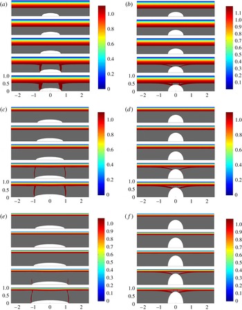
Figure 8. Speed distribution (
 $u$
) as the droplet gets larger. Rows represent constant Bingham number: (a,b)
$u$
) as the droplet gets larger. Rows represent constant Bingham number: (a,b)
 $B=5$
, (c,d)
$B=5$
, (c,d)
 $B=20$
, (e,f)
$B=20$
, (e,f)
 $B=50$
. (a,c,e)
$B=50$
. (a,c,e)
 $H=0.2$
(slender drop) and (b,d,f)
$H=0.2$
(slender drop) and (b,d,f)
 $L=0.5$
(fat drop). (a)
$L=0.5$
(fat drop). (a)
 $L=0.55$
, 0.6, 0.65, 0.675 and 0.7 (from top to bottom in the panel); (b)
$L=0.55$
, 0.6, 0.65, 0.675 and 0.7 (from top to bottom in the panel); (b)
 $H=0.3$
, 0.34, 0.375, 0.4 and 0.425; (c)
$H=0.3$
, 0.34, 0.375, 0.4 and 0.425; (c)
 $L=0.8$
, 0.85, 0.9, 0.925 and 1; (d)
$L=0.8$
, 0.85, 0.9, 0.925 and 1; (d)
 $H=0.5$
, 0.55, 0.575, 0.61 and 0.625; (e)
$H=0.5$
, 0.55, 0.575, 0.61 and 0.625; (e)
 $L=0.95$
, 1, 1.05, 1.15, 1.2 (f)
$L=0.95$
, 1, 1.05, 1.15, 1.2 (f)
 $H=0.6$
, 0.65, 0.69, 0.725 and 0.75.
$H=0.6$
, 0.65, 0.69, 0.725 and 0.75.
4.3. Encapsulation and failure
We have computed approximately 400 encapsulation flows, as described. These cover the approximate ranges
 $5<B<200$
,
$5<B<200$
,
 $0.025<H<0.9$
,
$0.025<H<0.9$
,
 $0.025<L<1.25$
. Figure 8 illustrates some of the general trends observed. For each row of computations the Bingham number is held constant. The left-hand column, (a,c,e) has
$0.025<L<1.25$
. Figure 8 illustrates some of the general trends observed. For each row of computations the Bingham number is held constant. The left-hand column, (a,c,e) has
 $L$
constant and
$L$
constant and
 $H$
varied; the right column (b,d,f) has
$H$
varied; the right column (b,d,f) has
 $H$
fixed and variable
$H$
fixed and variable
 $L$
. The colourmap plots the speed of the fluid, with the grey area denoting the unyielded plug. We observe that there essentially are two different regimes of plug breaking:
$L$
. The colourmap plots the speed of the fluid, with the grey area denoting the unyielded plug. We observe that there essentially are two different regimes of plug breaking:
- Slender droplets:
-
if the droplet aspect ratio
${\it\delta}=H/L$
is small (in other words the length of the drop is much larger than its width) then the plug appears to yield initially close to the two tips of the droplet (figure 8
a,c,e). - Fat droplets:
-
if the width of the droplet is similar to or larger than the length, the plug appears to yield closer to
$x=0$
, in the widest part of the droplet (figure 8
b,d,f).


This confirms that increasing either
 $L$
or
$L$
or
 $H$
will eventually yield the plug around the droplet, as was suggested by the rudimentary analysis in § 2.3. The other remarkable observation is that the yield surface position is approximately constant for the simulations shown in figure 8, up to and directly after the plug breaks (although of course with breaks after yielding). This implies that the stress distribution on the outside of the plug is not greatly affected by plug breaking. Thus, the deduction from the asymptotic analysis of the previous section, namely of a very small perturbation of the yield surface due to the droplet, appears to be valid for a broader range of aspect ratios
$H$
will eventually yield the plug around the droplet, as was suggested by the rudimentary analysis in § 2.3. The other remarkable observation is that the yield surface position is approximately constant for the simulations shown in figure 8, up to and directly after the plug breaks (although of course with breaks after yielding). This implies that the stress distribution on the outside of the plug is not greatly affected by plug breaking. Thus, the deduction from the asymptotic analysis of the previous section, namely of a very small perturbation of the yield surface due to the droplet, appears to be valid for a broader range of aspect ratios
 ${\it\delta}=H/L$
.
${\it\delta}=H/L$
.
To examine the breaking mechanism, we have plotted the various stresses in figure 9 for one sequence of slender drops (
 $B=20$
,
$B=20$
,
 $H=0.2$
and increasing
$H=0.2$
and increasing
 $L$
. The first noticeable feature is that as
$L$
. The first noticeable feature is that as
 $L$
increases through the breaking transition the distribution of stresses remains qualitatively similar. Thus, the breaking itself does not affect the overall pattern of stresses, which are dominated primarily by changes in droplet shape. Upstream and downstream of the droplet the stresses develop relatively quickly (within a channel width) and adopt distributions close to fully developed. The vertically oriented yielded regions (cracks?) coincide with a region within which the shear stress is focused:
$L$
increases through the breaking transition the distribution of stresses remains qualitatively similar. Thus, the breaking itself does not affect the overall pattern of stresses, which are dominated primarily by changes in droplet shape. Upstream and downstream of the droplet the stresses develop relatively quickly (within a channel width) and adopt distributions close to fully developed. The vertically oriented yielded regions (cracks?) coincide with a region within which the shear stress is focused:
 ${\it\tau}_{xy}$
becomes large and negative near the tips of the droplet. This is combined with significant extensional stresses
${\it\tau}_{xy}$
becomes large and negative near the tips of the droplet. This is combined with significant extensional stresses
 ${\it\tau}_{xx}=-{\it\tau}_{yy}$
. The basic mechanism appears to be that outlined in § 2.3. In the absence of extensional stresses, the pressure must transition from its shear-layer values to zero at the droplet surface. This driving force is evidently larger at the tips of the droplet. One way of reducing the burden on the change in
${\it\tau}_{xx}=-{\it\tau}_{yy}$
. The basic mechanism appears to be that outlined in § 2.3. In the absence of extensional stresses, the pressure must transition from its shear-layer values to zero at the droplet surface. This driving force is evidently larger at the tips of the droplet. One way of reducing the burden on the change in
 $p$
is by taking up a part of the pressure within the extensional stresses. For example, on the interface where it is nearly flat the normal stress condition is
$p$
is by taking up a part of the pressure within the extensional stresses. For example, on the interface where it is nearly flat the normal stress condition is
 $p={\it\tau}_{yy}$
and we can observe that
$p={\it\tau}_{yy}$
and we can observe that
 $|{\it\tau}_{yy}|$
becomes significant, changing sign towards the yield surface. In the centre of the droplets it appears that the distribution of
$|{\it\tau}_{yy}|$
becomes significant, changing sign towards the yield surface. In the centre of the droplets it appears that the distribution of
 ${\it\tau}_{xy}$
is shifted upwards by
${\it\tau}_{xy}$
is shifted upwards by
 $h(x)$
, but near to the ends of the droplet the stresses adapt to the far field in a relatively narrow region.
$h(x)$
, but near to the ends of the droplet the stresses adapt to the far field in a relatively narrow region.

Figure 9. Stress distribution as the droplet gets larger.
 $B=20$
,
$B=20$
,
 $H=0.2$
, and from top to bottom in each panel
$H=0.2$
, and from top to bottom in each panel
 $L=0.8$
, 0.85, 0.9, 0.925 and 1. (a) Speed; (b) pressure; (c)
$L=0.8$
, 0.85, 0.9, 0.925 and 1. (a) Speed; (b) pressure; (c)
 ${\it\tau}_{xy}$
; (d)
${\it\tau}_{xy}$
; (d)
 ${\it\tau}_{xx}$
; (e)
${\it\tau}_{xx}$
; (e)
 ${\it\sigma}_{xx}=-p+{\it\tau}_{xx}$
and (f)
${\it\sigma}_{xx}=-p+{\it\tau}_{xx}$
and (f)
 ${\it\sigma}_{yy}=-p+{\it\tau}_{yy}$
.
${\it\sigma}_{yy}=-p+{\it\tau}_{yy}$
.
The stress distributions in the case of fat droplets are illustrated in figure 10 for
 $B=20$
,
$B=20$
,
 $L=0.7$
. Although the far fields are similar to the slender droplet, the mechanism of breaking appears to be different. Again we have a transition as the droplet size is increased (now
$L=0.7$
. Although the far fields are similar to the slender droplet, the mechanism of breaking appears to be different. Again we have a transition as the droplet size is increased (now
 $H$
). Considering the second example in § 2.3 we might expect that
$H$
). Considering the second example in § 2.3 we might expect that
 $$\begin{eqnarray}\frac{\partial {\it\tau}_{xy}}{\partial y}\sim O\left(\frac{B}{y_{y}-H}\right)\end{eqnarray}$$
close to
 $x=0$
(within a layer that is getting progressively shorter). If we suppose that the pressure gradient is partly constrained by the far-field plane Poiseuille flow pressure gradient, then we might expect that the
$x=0$
(within a layer that is getting progressively shorter). If we suppose that the pressure gradient is partly constrained by the far-field plane Poiseuille flow pressure gradient, then we might expect that the
 $y$
-derivative of
$y$
-derivative of
 ${\it\tau}_{xy}$
is balanced by
${\it\tau}_{xy}$
is balanced by
 $x$
-derivatives in
$x$
-derivatives in
 ${\it\tau}_{xx}$
, which we observe in figure 10. The yielding appears to occur at the ends of the central shear layer.
${\it\tau}_{xx}$
, which we observe in figure 10. The yielding appears to occur at the ends of the central shear layer.

Figure 10. Stress distribution as the droplet gets larger.
 $B=20$
,
$B=20$
,
 $L=0.7$
, and from top to bottom in each panel
$L=0.7$
, and from top to bottom in each panel
 $H=0.5$
, 0.55, 0.575, 0.61 and 0.625. (a) Speed; (b) pressure; (c)
$H=0.5$
, 0.55, 0.575, 0.61 and 0.625. (a) Speed; (b) pressure; (c)
 ${\it\tau}_{xy}$
; (d)
${\it\tau}_{xy}$
; (d)
 ${\it\tau}_{xx}$
; (e)
${\it\tau}_{xx}$
; (e)
 ${\it\sigma}_{xx}$
and (f)
${\it\sigma}_{xx}$
and (f)
 ${\it\sigma}_{yy}$
.
${\it\sigma}_{yy}$
.
4.4. Perturbation of pressure
It is also insightful to quantify the perturbation of pressure as a result of insertion of the droplet inside the plug region. Figures 9 and 10 indicate that the distribution of the pressure perturbation is localized around the droplet positions. To quantify this we define
 $$\begin{eqnarray}{\it\phi}_{p}=\frac{|{\rm\Delta}p_{\{H,L\}}(-X,X)-{\rm\Delta}p_{\{0,0\}}(-X,X)|}{{\rm\Delta}p_{\{0,0\}}(-1,1)},\end{eqnarray}$$
where
 ${\rm\Delta}p_{\{H,L\}}(-X,X)$
is the pressure drop over the length
${\rm\Delta}p_{\{H,L\}}(-X,X)$
is the pressure drop over the length
 $[-X,X]$
computed with an elliptic droplet of size
$[-X,X]$
computed with an elliptic droplet of size
 $H$
and
$H$
and
 $L$
. Here
$L$
. Here
 $X$
is selected as our computational length (which is chosen to ensure the flow is fully developed between droplets; see the discussion in § 4.2). Thus,
$X$
is selected as our computational length (which is chosen to ensure the flow is fully developed between droplets; see the discussion in § 4.2). Thus,
 ${\rm\Delta}p_{\{0,0\}}(-X,X)$
represents the pressure drop over the same length in an unperturbed Poiseuille flow. This difference is normalized by the pressure drop
${\rm\Delta}p_{\{0,0\}}(-X,X)$
represents the pressure drop over the same length in an unperturbed Poiseuille flow. This difference is normalized by the pressure drop
 ${\rm\Delta}p_{\{0,0\}}(-1,1)$
, representing the pressure drop in Poiseuille flow over a length equivalent to the channel width.
${\rm\Delta}p_{\{0,0\}}(-1,1)$
, representing the pressure drop in Poiseuille flow over a length equivalent to the channel width.
Figure 11(a,b) shows variation of
 ${\it\phi}_{p}$
with respect to the size of drop as well as the yield stress (
${\it\phi}_{p}$
with respect to the size of drop as well as the yield stress (
 $B$
). Note that in each of the subplots the largest value of
$B$
). Note that in each of the subplots the largest value of
 $L$
or
$L$
or
 $H$
that is illustrated corresponds to a case for which the plug yields. Figure 11(a) is associated with slender drops where we see that the pressure perturbation is less than 1 % of the pressure scale (
$H$
that is illustrated corresponds to a case for which the plug yields. Figure 11(a) is associated with slender drops where we see that the pressure perturbation is less than 1 % of the pressure scale (
 ${\rm\Delta}p_{\{0,0\}}(-1,1)$
). However, the effect of droplet size is more significant in the case of fat droplets; see figure 11(b). This is probably linked to the different failure mechanisms observed already for slender and fat droplets. For droplets that do not break the plug
${\rm\Delta}p_{\{0,0\}}(-1,1)$
). However, the effect of droplet size is more significant in the case of fat droplets; see figure 11(b). This is probably linked to the different failure mechanisms observed already for slender and fat droplets. For droplets that do not break the plug
 ${\it\phi}_{p}$
remains rather small. It is of course intuitive in both cases that larger droplets lead to larger pressure perturbations. Equally, as remarked earlier, although increasing
${\it\phi}_{p}$
remains rather small. It is of course intuitive in both cases that larger droplets lead to larger pressure perturbations. Equally, as remarked earlier, although increasing
 $B$
increases the ability of the plug to resist yielding it also increases the frictional pressure drop, and hence the stress variation that must be accommodated within the plug.
$B$
increases the ability of the plug to resist yielding it also increases the frictional pressure drop, and hence the stress variation that must be accommodated within the plug.

Figure 11. Variation of pressure perturbation parameter
 ${\it\phi}_{p}$
with size of the droplet for different Bingham numbers (○,
${\it\phi}_{p}$
with size of the droplet for different Bingham numbers (○,
 $B=5$
; ▫,
$B=5$
; ▫,
 $B=20$
; ▵,
$B=20$
; ▵,
 $B=50$
). (a) Drops with varying length and constant height (
$B=50$
). (a) Drops with varying length and constant height (
 $H=0.2$
) and (b) drops with varying height and constant length (
$H=0.2$
) and (b) drops with varying height and constant length (
 $L=0.5$
). In each subplot the largest value of
$L=0.5$
). In each subplot the largest value of
 $L$
or
$L$
or
 $H$
corresponds to a case with a yielded plug.
$H$
corresponds to a case with a yielded plug.
4.5. Maximum size of encapsulated droplets
By successively iterating with respect to
 $H$
and
$H$
and
 $L$
we are able to approximately determine the limiting size of droplet that can remain encapsulated within the plug region. Figure 12 shows the critical values in the
$L$
we are able to approximately determine the limiting size of droplet that can remain encapsulated within the plug region. Figure 12 shows the critical values in the
 $(L,H)$
-plane for five different values of Bingham number,
$(L,H)$
-plane for five different values of Bingham number,
 $B$
. This plot is the conclusion of approximately 400 different simulations. For a given Bingham number, any drop lying below the associated curve does not break the plug region. We see that for any Bingham number (no matter how large) we have maximum values for the length and height of the droplet. The maximum height is mostly limited by the plug width. Although there is no similar simple physical limit for the maximum length, we still see that the growth of stresses for long droplets yields the plug. In fact the shape of the curves at small
$B$
. This plot is the conclusion of approximately 400 different simulations. For a given Bingham number, any drop lying below the associated curve does not break the plug region. We see that for any Bingham number (no matter how large) we have maximum values for the length and height of the droplet. The maximum height is mostly limited by the plug width. Although there is no similar simple physical limit for the maximum length, we still see that the growth of stresses for long droplets yields the plug. In fact the shape of the curves at small
 $H$
indicates that for slender droplets the encapsulation becomes very sensitive to changes in the length, i.e. small increases in the length can break the plug (see also figure 9
a,c,e).
$H$
indicates that for slender droplets the encapsulation becomes very sensitive to changes in the length, i.e. small increases in the length can break the plug (see also figure 9
a,c,e).

Figure 12. Maximum size of encapsulated droplets, computed for five different
 $B$
: ○,
$B$
: ○,
 $B=5$
; ▫,
$B=5$
; ▫,
 $B=10$
; ▵,
$B=10$
; ▵,
 $B=20$
; ♢,
$B=20$
; ♢,
 $B=50$
;
$B=50$
;
 $B=200$
.
$B=200$
.
A last observation here is that the increase in size of droplet with
 $B$
is much less than linear. Therefore, just increasing the yield stress of the encapsulating fluid does not allow correspondingly large droplets. The underlying reasons why seem to be captured in the simple analysis of § 2.3. Long droplets break near the ends. Breaking arises from the need to bridge the discrepancy between non-zero (frictional) pressures in the yielded fluid layers and zero normal stress on the droplet surface. This discrepancy increases with
$B$
is much less than linear. Therefore, just increasing the yield stress of the encapsulating fluid does not allow correspondingly large droplets. The underlying reasons why seem to be captured in the simple analysis of § 2.3. Long droplets break near the ends. Breaking arises from the need to bridge the discrepancy between non-zero (frictional) pressures in the yielded fluid layers and zero normal stress on the droplet surface. This discrepancy increases with
 $L$
but also with
$L$
but also with
 $B$
, i.e. the frictional pressure scales like
$B$
, i.e. the frictional pressure scales like
 $xB/y_{y,0}$
. It is unclear what the asymptotic behaviour might be as
$xB/y_{y,0}$
. It is unclear what the asymptotic behaviour might be as
 $B\rightarrow \infty$
. If we assume that the pressure discrepancy provides the main stress scale for
$B\rightarrow \infty$
. If we assume that the pressure discrepancy provides the main stress scale for
 ${\it\tau}$
, we would expect the limiting lengths to satisfy
${\it\tau}$
, we would expect the limiting lengths to satisfy
 $L\sim O(y_{y,0})\sim O(1-(\sqrt{2}/B^{1/2}))$
as
$L\sim O(y_{y,0})\sim O(1-(\sqrt{2}/B^{1/2}))$
as
 $B\rightarrow \infty$
, i.e. a finite limit would be attained. This analysis may be too simplistic.
$B\rightarrow \infty$
, i.e. a finite limit would be attained. This analysis may be too simplistic.
5. Encapsulation with fluids of different densities
We now explore the effect of allowing a density difference between the fluids. Assuming the encapsulated fluid remains in steady rigid motion, the pressure field within the droplet is
 $p={\it\chi}x+\text{const.}$
, where we recall that
$p={\it\chi}x+\text{const.}$
, where we recall that
 ${\it\chi}=(\hat{{\it\rho}}_{d}-\hat{{\it\rho}}){\hat{g}}\hat{R}^{2}/(\hat{{\it\mu}}\hat{U} _{0})$
represents the competition between buoyant and viscous stresses. Considering the preceding discussion and the simple analysis in § 2.3, an intuitive notion is that by selecting
${\it\chi}=(\hat{{\it\rho}}_{d}-\hat{{\it\rho}}){\hat{g}}\hat{R}^{2}/(\hat{{\it\mu}}\hat{U} _{0})$
represents the competition between buoyant and viscous stresses. Considering the preceding discussion and the simple analysis in § 2.3, an intuitive notion is that by selecting
 ${\it\chi}=-B/y_{y,0}$
the pressure gradient in the droplet would match that in the yielded fluid layers. This would eliminate the need for normal stress gradients across the plug, and hence presumably reduce
${\it\chi}=-B/y_{y,0}$
the pressure gradient in the droplet would match that in the yielded fluid layers. This would eliminate the need for normal stress gradients across the plug, and hence presumably reduce
 ${\it\tau}$
.
${\it\tau}$
.
We test the above notion computationally. The code described earlier is adapted by discretizing both the droplet and carrier fluid domains. The additional body force term
 ${\it\chi}$
can be added to the droplet
${\it\chi}$
can be added to the droplet
 $x$
-momentum equation (or instead
$x$
-momentum equation (or instead
 $-{\it\chi}$
added to the carrier fluid equations). Different fluid properties are assigned in each domain (e.g.
$-{\it\chi}$
added to the carrier fluid equations). Different fluid properties are assigned in each domain (e.g.
 $B=0$
is inside the droplet) and the Stokes flow solution is computed on both domains simultaneously using the augmented Lagrangian algorithm described earlier.
$B=0$
is inside the droplet) and the Stokes flow solution is computed on both domains simultaneously using the augmented Lagrangian algorithm described earlier.
Firstly, we address the question of whether the density difference might significantly affect breaking of the plug region. Figure 13(a) shows the maximum height
 $H$
before the plug yields, for two droplets with different
$H$
before the plug yields, for two droplets with different
 $L$
at
$L$
at
 $B=20$
. We observe that the shorter droplet (
$B=20$
. We observe that the shorter droplet (
 $L=0.4$
) is relatively insensitive to
$L=0.4$
) is relatively insensitive to
 ${\it\chi}$
, whereas the longer droplet (
${\it\chi}$
, whereas the longer droplet (
 $L=1.75$
) shows remarkable sensitivity. Sensitivity to
$L=1.75$
) shows remarkable sensitivity. Sensitivity to
 $L$
per se is to be expected as the effect of
$L$
per se is to be expected as the effect of
 ${\it\chi}$
naturally amplifies with
${\it\chi}$
naturally amplifies with
 $x$
(or
$x$
(or
 $L$
), due to the channel orientation. We see that if the droplet is heavier than the carrier fluid (
$L$
), due to the channel orientation. We see that if the droplet is heavier than the carrier fluid (
 ${\it\chi}>0$
), encapsulation fails at a smaller size for the drop. On the other hand, for a lighter droplet (
${\it\chi}>0$
), encapsulation fails at a smaller size for the drop. On the other hand, for a lighter droplet (
 ${\it\chi}<0$
) buoyancy tends to stabilize the encapsulation, allowing larger drops to be successfully encapsulated. For the case shown in figure 13(a), in which
${\it\chi}<0$
) buoyancy tends to stabilize the encapsulation, allowing larger drops to be successfully encapsulated. For the case shown in figure 13(a), in which
 $B=20$
, we see that maximum size of the drop happens at
$B=20$
, we see that maximum size of the drop happens at
 ${\it\chi}\approx -27$
to
${\it\chi}\approx -27$
to
 $-28$
. This approximately coincides with the frictional pressure gradient of the plane Poiseuille flow (for
$-28$
. This approximately coincides with the frictional pressure gradient of the plane Poiseuille flow (for
 $B=20$
we find
$B=20$
we find
 $\partial p/\partial x=-B/y_{y,0}\approx -27.8$
). Thus, the notion that selecting
$\partial p/\partial x=-B/y_{y,0}\approx -27.8$
). Thus, the notion that selecting
 ${\it\chi}\approx -B/y_{y,0}$
may provide an optimal size of encapsulated droplet appears reasonable. Essentially, buoyancy acts to balance the frictional pressure losses for
${\it\chi}\approx -B/y_{y,0}$
may provide an optimal size of encapsulated droplet appears reasonable. Essentially, buoyancy acts to balance the frictional pressure losses for
 ${\it\chi}>-B/y_{y,0}$
, but on decreasing
${\it\chi}>-B/y_{y,0}$
, but on decreasing
 ${\it\chi}$
still further strong buoyancy forces act to exert stress on the plug.
${\it\chi}$
still further strong buoyancy forces act to exert stress on the plug.

Figure 13.
 $B=20$
. (a) Variation of maximum height (maximum
$B=20$
. (a) Variation of maximum height (maximum
 $H$
which does not break the plug) for two different lengths of drop (▫,
$H$
which does not break the plug) for two different lengths of drop (▫,
 $L=0.4$
and ○,
$L=0.4$
and ○,
 $L=1.75$
) with density difference (
$L=1.75$
) with density difference (
 ${\it\chi}$
). (b) Maximum size of drop for three different
${\it\chi}$
). (b) Maximum size of drop for three different
 ${\it\chi}$
: ○,
${\it\chi}$
: ○,
 $=20$
; ▫,
$=20$
; ▫,
 ${\it\chi}=0$
; ▵,
${\it\chi}=0$
; ▵,
 ${\it\chi}=-20$
.
${\it\chi}=-20$
.
Note that although the normal stress discrepancy may be reduced for
 ${\it\chi}\approx -B/y_{y,0}$
, the tangential stresses in the plug are still perturbed by the presence of the droplet. Thus, the droplet may still break the plug. Figure 13(b) shows the critical values of
${\it\chi}\approx -B/y_{y,0}$
, the tangential stresses in the plug are still perturbed by the presence of the droplet. Thus, the droplet may still break the plug. Figure 13(b) shows the critical values of
 $H$
and
$H$
and
 $L$
for
$L$
for
 $B=20$
, above which the plug yields, for three different
$B=20$
, above which the plug yields, for three different
 ${\it\chi}=-20$
, 0 and 20. Again we see that a favourable density difference (lighter droplets) allows the encapsulation of longer drops, whereas an unfavourable density difference (heavier droplets) weakens the encapsulation capabilities.
${\it\chi}=-20$
, 0 and 20. Again we see that a favourable density difference (lighter droplets) allows the encapsulation of longer drops, whereas an unfavourable density difference (heavier droplets) weakens the encapsulation capabilities.
Figure 14 explores variations in the stress fields as the density of the droplet is varied. The plug close to the central part of the droplet is largely unaffected by
 ${\it\chi}$
, but on increasing
${\it\chi}$
, but on increasing
 $|x|$
we observe generation of extensional stresses towards the ends of the droplet within the plug (figure 14
d). Increasing
$|x|$
we observe generation of extensional stresses towards the ends of the droplet within the plug (figure 14
d). Increasing
 ${\it\chi}$
amplifies the size of extensional stresses and of the pressure in these regions (figure 14
b,d). The stresses combine so that
${\it\chi}$
amplifies the size of extensional stresses and of the pressure in these regions (figure 14
b,d). The stresses combine so that
 ${\it\sigma}_{yy}$
shows little variation in
${\it\sigma}_{yy}$
shows little variation in
 $y$
(figure 14
f), which implies that the pressure variation in
$y$
(figure 14
f), which implies that the pressure variation in
 $y$
is negatively amplified in
$y$
is negatively amplified in
 ${\it\tau}_{xx}$
. The net effect is that the front of the droplet is stretched and the rear is compressed (in the
${\it\tau}_{xx}$
. The net effect is that the front of the droplet is stretched and the rear is compressed (in the
 $x$
direction); see figure 14(e). These normal stress gradient results in significant shear stresses (figure 14
c). The underlying pattern is not changed for
$x$
direction); see figure 14(e). These normal stress gradient results in significant shear stresses (figure 14
c). The underlying pattern is not changed for
 ${\it\chi}>0$
, but simply amplified.
${\it\chi}>0$
, but simply amplified.

Figure 14. Stress distribution as the droplet becomes heavier:
 $B=20$
,
$B=20$
,
 $L=0.9$
and
$L=0.9$
and
 $H=0.2$
. From top to bottom in each panel:
$H=0.2$
. From top to bottom in each panel:
 ${\it\chi}=-10$
,
${\it\chi}=-10$
,
 $-1$
, 0, 1 and 10. (a) Speed; (b) pressure; (c)
$-1$
, 0, 1 and 10. (a) Speed; (b) pressure; (c)
 ${\it\tau}_{xy}$
; (d)
${\it\tau}_{xy}$
; (d)
 ${\it\tau}_{xx}$
; (e)
${\it\tau}_{xx}$
; (e)
 ${\it\sigma}_{xx}$
and (f)
${\it\sigma}_{xx}$
and (f)
 ${\it\sigma}_{yy}$
.
${\it\sigma}_{yy}$
.
6. Droplet encapsulation in a pipe
For the purposes of practical application we now consider the analogous flow to that described in § 2, but within a vertical pipe of radius
 $\hat{R}$
. We describe the problem in a cylindrical coordinate system, assuming that the flow is axisymmetric with droplets travelling along the pipe axis. As in § 2 a moving coordinate system is adopted. Lengths and velocities are scaled with
$\hat{R}$
. We describe the problem in a cylindrical coordinate system, assuming that the flow is axisymmetric with droplets travelling along the pipe axis. As in § 2 a moving coordinate system is adopted. Lengths and velocities are scaled with
 $\hat{R}$
and
$\hat{R}$
and
 ${\hat{W}}_{0}$
respectively, where
${\hat{W}}_{0}$
respectively, where
 ${\hat{W}}_{0}$
is the mean velocity along the pipe, i.e. the flow rate is
${\hat{W}}_{0}$
is the mean velocity along the pipe, i.e. the flow rate is
 ${\rm\pi}\hat{R}^{2}{\hat{W}}_{0}$
. Denoting by
${\rm\pi}\hat{R}^{2}{\hat{W}}_{0}$
. Denoting by
 ${\hat{W}}_{p}$
the fully developed plug velocity of the Hagen–Poiseuille flow (with no droplets), the variables are as follows:
${\hat{W}}_{p}$
the fully developed plug velocity of the Hagen–Poiseuille flow (with no droplets), the variables are as follows:
 $$\begin{eqnarray}(r,z,{\it\theta})=\left(\frac{\hat{r}}{\hat{R}},\frac{\hat{z}-{\hat{W}}_{p}\hat{t}}{\hat{R}},{\it\theta}\right),\quad (u,w)=\left(\frac{\hat{u} _{r}}{{\hat{W}}_{0}},\frac{\hat{u} _{z}-{\hat{W}}_{p}}{{\hat{W}}_{0}}\right),\end{eqnarray}$$
and
 $t={\hat{W}}_{p}\hat{t}/\hat{R}$
. The deviatoric stresses are scaled with
$t={\hat{W}}_{p}\hat{t}/\hat{R}$
. The deviatoric stresses are scaled with
 $\hat{{\it\mu}}{\hat{W}}_{0}/\hat{R}$
as is the modified pressure (on subtracting the static pressure of the carrier fluid),
$\hat{{\it\mu}}{\hat{W}}_{0}/\hat{R}$
as is the modified pressure (on subtracting the static pressure of the carrier fluid),
 $$\begin{eqnarray}\hat{p}=\hat{p}_{0}+\hat{{\it\rho}}{\hat{g}}\hat{z}+\frac{\hat{{\it\mu}}{\hat{W}}_{0}}{\hat{R}}p.\end{eqnarray}$$
Exploiting axisymmetry of the geometry, the dimensionless forms of the continuity and momentum equations governing carrier fluid are
 $$\begin{eqnarray}\displaystyle & \displaystyle \frac{1}{r}\frac{\partial }{\partial r}(ru)+\frac{\partial w}{\partial z}=0, & \displaystyle\end{eqnarray}$$
 $$\begin{eqnarray}\displaystyle & \displaystyle \mathit{Re}\left(u\frac{\partial w}{\partial r}+w\frac{\partial w}{\partial z}\right)=-\frac{\partial p}{\partial z}+\frac{1}{r}\frac{\partial }{\partial r}(r{\it\tau}_{rz})+\frac{\partial {\it\tau}_{zz}}{\partial z}, & \displaystyle\end{eqnarray}$$
 $$\begin{eqnarray}\displaystyle & \displaystyle \mathit{Re}\left(u\frac{\partial u}{\partial r}+w\frac{\partial u}{\partial z}\right)=-\frac{\partial p}{\partial r}+\frac{1}{r}\frac{\partial }{\partial r}(r{\it\tau}_{rr})+\frac{\partial {\it\tau}_{rz}}{\partial z}-\frac{{\it\tau}_{{\it\theta}{\it\theta}}}{r}. & \displaystyle\end{eqnarray}$$
 $\dot{{\it\gamma}}=\sqrt{\dot{{\it\gamma}}_{rr}^{2}+\dot{{\it\gamma}}_{zz}^{2}+\dot{{\it\gamma}}_{{\it\theta}{\it\theta}}^{2}+2\dot{{\it\gamma}}_{rz}^{2}}$
is the rate of strain, and
$\dot{{\it\gamma}}=\sqrt{\dot{{\it\gamma}}_{rr}^{2}+\dot{{\it\gamma}}_{zz}^{2}+\dot{{\it\gamma}}_{{\it\theta}{\it\theta}}^{2}+2\dot{{\it\gamma}}_{rz}^{2}}$
is the rate of strain, and
 ${\it\tau}=\sqrt{{\it\tau}_{rr}^{2}+{\it\tau}_{zz}^{2}+{\it\tau}_{{\it\theta}{\it\theta}}^{2}+2{\it\tau}_{rz}^{2}}$
is the deviatoric stress. The components are given by
${\it\tau}=\sqrt{{\it\tau}_{rr}^{2}+{\it\tau}_{zz}^{2}+{\it\tau}_{{\it\theta}{\it\theta}}^{2}+2{\it\tau}_{rz}^{2}}$
is the deviatoric stress. The components are given by  $$\begin{eqnarray}\dot{{\it\gamma}}_{rr}=2\frac{\partial u}{\partial r},\quad \dot{{\it\gamma}}_{{\it\theta}{\it\theta}}=2\frac{w}{r},\quad \dot{{\it\gamma}}_{zz}=2\frac{\partial w}{\partial z},\quad \dot{{\it\gamma}}_{rz}=\dot{{\it\gamma}}_{zr}=\frac{\partial w}{\partial r}+\frac{\partial u}{\partial z}.\end{eqnarray}$$
Reynolds number and Bingham number are defined as
 $\mathit{Re}=\hat{{\it\rho}}{\hat{W}}_{0}\hat{R}/\hat{{\it\mu}}$
and
$\mathit{Re}=\hat{{\it\rho}}{\hat{W}}_{0}\hat{R}/\hat{{\it\mu}}$
and
 $B=\hat{{\it\tau}}_{Y}\hat{R}/(\hat{{\it\mu}}{\hat{W}}_{0})$
.
$B=\hat{{\it\tau}}_{Y}\hat{R}/(\hat{{\it\mu}}{\hat{W}}_{0})$
.
As before, we consider a single droplet from our periodic train of droplets. The scaled droplet length is
 $L$
and the maximal radius is
$L$
and the maximal radius is
 $H$
. The droplet surface is steady within the moving fame of reference and is denoted
$H$
. The droplet surface is steady within the moving fame of reference and is denoted
 $r=h(z)$
. Within the droplet the following equations must be satisfied:
$r=h(z)$
. Within the droplet the following equations must be satisfied:
 $$\begin{eqnarray}\displaystyle & \displaystyle \frac{1}{r}\frac{\partial }{\partial r}(ru)+\frac{\partial w}{\partial z}=0, & \displaystyle\end{eqnarray}$$
 $$\begin{eqnarray}\displaystyle & \displaystyle {\it\phi}\mathit{Re}\left(u\frac{\partial w}{\partial r}+w\frac{\partial w}{\partial z}\right)=-\frac{\partial p}{\partial z}+m\frac{1}{r}\frac{\partial }{\partial r}\left(r\frac{\partial w}{\partial r}\right)+m\frac{\partial ^{2}w}{\partial z^{2}}+{\it\chi}, & \displaystyle\end{eqnarray}$$
 $$\begin{eqnarray}\displaystyle & \displaystyle {\it\phi}\mathit{Re}\left(u\frac{\partial u}{\partial r}+w\frac{\partial u}{\partial z}\right)=-\frac{\partial p}{\partial r}+m\frac{1}{r}\frac{\partial }{\partial r}\left(r\frac{\partial u}{\partial r}\right)+m\frac{\partial ^{2}u}{\partial z^{2}}-m\frac{u}{r^{2}}, & \displaystyle\end{eqnarray}$$
 ${\it\chi}=((\hat{{\it\rho}}_{d}-\hat{{\it\rho}}){\hat{g}}\hat{R}^{2})/({\hat{W}}_{0}\hat{{\it\mu}})$
. Similar boundary and interfacial conditions are satisfied as for the plane channel problem earlier. As before, it is assumed that the droplet translates uniformly within the moving plug.
${\it\chi}=((\hat{{\it\rho}}_{d}-\hat{{\it\rho}}){\hat{g}}\hat{R}^{2})/({\hat{W}}_{0}\hat{{\it\mu}})$
. Similar boundary and interfacial conditions are satisfied as for the plane channel problem earlier. As before, it is assumed that the droplet translates uniformly within the moving plug.
6.1. Poiseuille flow solution
In a fixed frame of reference the Hagen–Poiseuille solution is easily found:
 $$\begin{eqnarray}W_{p}(r)=\left\{\begin{array}{@{}ll@{}}w_{p,0}\quad & \text{if }r\leqslant r_{y,0},\\ \displaystyle w_{p,0}\left[1-\left(\frac{r-r_{y,0}}{1-r_{y,0}}\right)^{2}\right]\quad & \text{if }r\geqslant r_{y,0},\end{array}\right.\end{eqnarray}$$
where
 $w_{p,0}=(B/(2r_{y,0}))(1-r_{y,0})^{2}$
. On imposing the flow rate constraint we find that the yield surface position satisfies the following Buckingham equation:
$w_{p,0}=(B/(2r_{y,0}))(1-r_{y,0})^{2}$
. On imposing the flow rate constraint we find that the yield surface position satisfies the following Buckingham equation:
 $$\begin{eqnarray}r_{y,0}^{4}-4r_{y,0}\left(1+\frac{3}{B}\right)+3=0,\end{eqnarray}$$
which has a unique zero in the interval
 $(0,1)$
.
$(0,1)$
.
6.2. Slender drop
For practical reasons it is advantageous to know if encapsulated droplets within a pipe flow also result in vanishing small perturbations of the flow streamlines. Thus, similar to § 3 we rescale the problem assuming a small slender droplet:
 $$\begin{eqnarray}r=R,\quad {\it\theta}={\it\Theta},\quad z{\it\delta}=Z,\quad u={\it\delta}U,\quad w=W,\quad p{\it\delta}=P.\end{eqnarray}$$
Upon rescaling and neglecting the inertial terms, the governing equations are
 $$\begin{eqnarray}\displaystyle & \displaystyle \frac{1}{R}\frac{\partial }{\partial R}(RU)+\frac{\partial W}{\partial Z}=0, & \displaystyle\end{eqnarray}$$
 $$\begin{eqnarray}\displaystyle & \displaystyle 0=-\frac{\partial P}{\partial Z}+\frac{1}{R}\frac{\partial }{\partial R}(R{\it\tau}_{RZ})+{\it\delta}^{2}\frac{\partial {\it\tau}_{ZZ}}{\partial Z}, & \displaystyle\end{eqnarray}$$
 $$\begin{eqnarray}\displaystyle & \displaystyle 0=-\frac{\partial P}{\partial R}+{\it\delta}^{2}\frac{1}{R}\frac{\partial }{\partial R}(R{\it\tau}_{RR})+{\it\delta}^{2}\frac{\partial {\it\tau}_{RZ}}{\partial Z}-{\it\delta}^{2}\frac{{\it\tau}_{{\it\Theta}{\it\Theta}}}{R}, & \displaystyle\end{eqnarray}$$
 ${\it\tau}_{rz}={\it\tau}_{RZ}$
,
${\it\tau}_{rz}={\it\tau}_{RZ}$
,
 ${\it\tau}_{rr}={\it\delta}{\it\tau}_{RR}$
,
${\it\tau}_{rr}={\it\delta}{\it\tau}_{RR}$
,
 ${\it\tau}_{{\it\theta}{\it\theta}}={\it\delta}{\it\tau}_{{\it\Theta}{\it\Theta}}$
and
${\it\tau}_{{\it\theta}{\it\theta}}={\it\delta}{\it\tau}_{{\it\Theta}{\it\Theta}}$
and
 ${\it\tau}_{zz}={\it\delta}{\it\tau}_{ZZ}$
. The constitutive relations are similar to (2.5), except that now
${\it\tau}_{zz}={\it\delta}{\it\tau}_{ZZ}$
. The constitutive relations are similar to (2.5), except that now  $$\begin{eqnarray}\displaystyle & {\it\tau}=\sqrt{{\it\tau}_{RZ}^{2}+{\it\delta}^{2}{\it\tau}_{RR}^{2}+{\it\delta}^{2}{\it\tau}_{{\it\Theta}{\it\Theta}}^{2}+{\it\delta}^{2}{\it\tau}_{ZZ}^{2}}, & \displaystyle\end{eqnarray}$$
 $$\begin{eqnarray}\displaystyle & \dot{{\it\gamma}}=\sqrt{\dot{{\it\gamma}}_{RZ}^{2}+{\it\delta}^{2}\dot{{\it\gamma}}_{RR}^{2}+{\it\delta}^{2}\dot{{\it\gamma}}_{{\it\Theta}{\it\Theta}}^{2}+{\it\delta}^{2}\dot{{\it\gamma}}_{ZZ}^{2}} & \displaystyle\end{eqnarray}$$
 $$\begin{eqnarray}\displaystyle \dot{{\it\gamma}}_{RZ} & = & \displaystyle \frac{\partial W}{\partial R}+{\it\delta}^{2}\frac{\partial U}{\partial Z},\end{eqnarray}$$
 $$\begin{eqnarray}\displaystyle \dot{{\it\gamma}}_{RR} & = & \displaystyle 2\frac{\partial U}{\partial R},\end{eqnarray}$$
 $$\begin{eqnarray}\displaystyle \dot{{\it\gamma}}_{{\it\Theta}{\it\Theta}} & = & \displaystyle 2\frac{W}{R},\end{eqnarray}$$
 $$\begin{eqnarray}\displaystyle \dot{{\it\gamma}}_{ZZ} & = & \displaystyle 2\frac{\partial W}{\partial Z}.\end{eqnarray}$$
We adopt a regular perturbation expansion in
 ${\it\delta}$
:
${\it\delta}$
:
 $(P,W,U)=(P_{0},W_{0},U_{0})+{\it\delta}(P_{1},W_{1},U_{1})+\cdots \!,$
substitute into the equations and derive the following leading-order problem:
$(P,W,U)=(P_{0},W_{0},U_{0})+{\it\delta}(P_{1},W_{1},U_{1})+\cdots \!,$
substitute into the equations and derive the following leading-order problem:
 $$\begin{eqnarray}\displaystyle & \displaystyle \frac{1}{R}\frac{\partial }{\partial R}(RU)+\frac{\partial W}{\partial Z}=0, & \displaystyle\end{eqnarray}$$
 $$\begin{eqnarray}\displaystyle & \displaystyle 0=-\frac{\partial P}{\partial Z}+\frac{1}{R}\frac{\partial }{\partial R}(R{\it\tau}_{RZ}), & \displaystyle\end{eqnarray}$$
 $$\begin{eqnarray}\displaystyle & \displaystyle 0=-\frac{\partial P}{\partial R}. & \displaystyle\end{eqnarray}$$
 $R=h$
yields
$R=h$
yields  $$\begin{eqnarray}{\it\tau}_{RZ}=\frac{\partial W_{0}}{\partial R}+B\,\text{sgn}\left(\frac{\partial W_{0}}{\partial R}\right)=\frac{\partial W_{0}}{\partial R}-B=\frac{1}{2}\frac{\partial P}{\partial Z}\left(R-\frac{h^{2}}{R}\right),\end{eqnarray}$$
and defining the yield surface
 $R=R_{y}$
as where
$R=R_{y}$
as where
 ${\it\tau}_{RZ}=-B$
we find
${\it\tau}_{RZ}=-B$
we find
 $$\begin{eqnarray}\frac{\partial W_{0}}{\partial R}=\frac{1}{2}\frac{\partial P}{\partial Z}\left(R-R_{y}-\frac{h^{2}}{R}+\frac{h^{2}}{R_{y}}\right),\quad \frac{\partial P}{\partial Z}=-\frac{2BR_{y}}{R_{y}^{2}-h^{2}}.\end{eqnarray}$$
We can reconstruct the velocity in the fixed frame, using the no-slip condition at
 $R=1$
:
$R=1$
:
 $$\begin{eqnarray}\displaystyle & & \displaystyle W_{0}(r)+w_{p,0}\nonumber\\ \displaystyle & & \displaystyle \quad =\left\{\begin{array}{@{}ll@{}}w_{p}\quad & \text{if}~0\leqslant R\leqslant R_{y},\\ \displaystyle w_{p}\left[1-\left(\frac{0.5(R-R_{y})^{2}+h^{2}(R-R_{y})/R_{y}+h^{2}\ln (R_{y}/R)}{0.5(1-R_{y})^{2}+h^{2}(1-R_{y})/R_{y}+h^{2}\ln R_{y}}\right)\right]\quad & \text{if}~R_{y}\leqslant R\leqslant 1,\end{array}\right.\nonumber\\ \displaystyle & & \displaystyle\end{eqnarray}$$
where the plug velocity is given by
 $$\begin{eqnarray}w_{p}=B\frac{R_{y}}{R_{y}^{2}-h^{2}}\left(\frac{(1-R_{y})^{2}}{2}+\frac{h^{2}}{R_{y}}(1-R_{y})+h^{2}\ln R_{y}\right).\end{eqnarray}$$
Finally we use the unit flow rate condition to find the pressure gradient (equivalently
 $R_{y}$
). This leads to the following Buckingham equation:
$R_{y}$
). This leads to the following Buckingham equation:
 $$\begin{eqnarray}R_{y}^{4}-4\left(1+\frac{3}{B}\right)R_{y}+3+\frac{2h^{2}}{R_{y}}\left[(1-R_{y})^{2}(2+R_{y})+\frac{6}{B}\right]=0,\end{eqnarray}$$
which may be solved numerically for
 $R_{y}$
.
$R_{y}$
.
Comparing the solution above with that in § 6.1, we note that the leading-order plug velocity, velocity profile and Buckingham equation are all
 $O(h^{2})$
perturbations from the unperturbed Poiseuille flow solution, cf. (6.15) and (6.17), (6.6) and (6.7), ….
$O(h^{2})$
perturbations from the unperturbed Poiseuille flow solution, cf. (6.15) and (6.17), (6.6) and (6.7), ….
The implications of this are two-fold. Firstly, in terms of the perturbation procedure there is no need to seek a correction to the solution at first order in
 ${\it\delta}$
. In practical terms, this means that for any small slender drop of aspect ratio
${\it\delta}$
. In practical terms, this means that for any small slender drop of aspect ratio
 ${\it\delta}$
the streamlines in the yielded layer will be perturbed by
${\it\delta}$
the streamlines in the yielded layer will be perturbed by
 $O({\it\delta}^{2})$
, suggesting that inertial effects on the flow are of
$O({\it\delta}^{2})$
, suggesting that inertial effects on the flow are of
 $O({\it\delta}^{2}\mathit{Re})$
as for the channel flow. Secondly, this suggests that a perturbation approximation of the above form would only require a first-order correction when
$O({\it\delta}^{2}\mathit{Re})$
as for the channel flow. Secondly, this suggests that a perturbation approximation of the above form would only require a first-order correction when
 $h\sim {\it\delta}^{1/2}$
. As
$h\sim {\it\delta}^{1/2}$
. As
 ${\it\delta}=H/L$
is the droplet aspect ratio, this suggests
${\it\delta}=H/L$
is the droplet aspect ratio, this suggests
 $L\sim {\it\delta}^{-1/2}$
. This hints that longer and wider droplets may be accommodated in the pipe geometry.
$L\sim {\it\delta}^{-1/2}$
. This hints that longer and wider droplets may be accommodated in the pipe geometry.

Figure 15. Stress distribution in the axisymmetric geometry as the droplet gets longer:
 $B=20$
,
$B=20$
,
 $H=0.4$
and from top to bottom in each panel
$H=0.4$
and from top to bottom in each panel
 $L=1.2$
, 1.25, 1.3, 1.34 and 1.45. (a) Velocity; (b) pressure; (c)
$L=1.2$
, 1.25, 1.3, 1.34 and 1.45. (a) Velocity; (b) pressure; (c)
 ${\it\tau}_{rz}$
; (d)
${\it\tau}_{rz}$
; (d)
 ${\it\tau}_{zz}$
; (e)
${\it\tau}_{zz}$
; (e)
 ${\it\tau}_{rr}$
and (f)
${\it\tau}_{rr}$
and (f)
 ${\it\tau}_{{\it\theta}{\it\theta}}$
.
${\it\tau}_{{\it\theta}{\it\theta}}$
.

Figure 16. Stress distribution in the axisymmetric geometry as the droplet height is increased:
 $B=20$
,
$B=20$
,
 $L=0.5$
and from top to bottom in each panel
$L=0.5$
and from top to bottom in each panel
 $H=0.4$
, 0.45, 0.5, 0.525 and 0.55. (a) Velocity; (b) pressure; (c)
$H=0.4$
, 0.45, 0.5, 0.525 and 0.55. (a) Velocity; (b) pressure; (c)
 ${\it\tau}_{rz}$
; (d)
${\it\tau}_{rz}$
; (d)
 ${\it\tau}_{zz}$
; (e)
${\it\tau}_{zz}$
; (e)
 ${\it\tau}_{rr}$
and (f)
${\it\tau}_{rr}$
and (f)
 ${\it\tau}_{{\it\theta}{\it\theta}}$
.
${\it\tau}_{{\it\theta}{\it\theta}}$
.
6.3. Examples of encapsulation and failure
We now present computed solutions of droplets as either
 $L$
or
$L$
or
 $H$
is increased until breaking point. Figure 15 shows yielding of the ‘slender’ droplet and figure 16 shows the ‘fat’ droplet. Superficially, the yielding mechanism is similar to the channel flow in which the plugs break (ends or near the centre). However, as suggested by the previous section, the plugs generally break at larger values of
$H$
is increased until breaking point. Figure 15 shows yielding of the ‘slender’ droplet and figure 16 shows the ‘fat’ droplet. Superficially, the yielding mechanism is similar to the channel flow in which the plugs break (ends or near the centre). However, as suggested by the previous section, the plugs generally break at larger values of
 $H$
and
$H$
and
 $L$
.
$L$
.
The main reason is in the normal stresses. The pressure distributions found are qualitatively similar between pipe and channel geometries. At the yield surface in the channel
 $-{\it\sigma}_{yy}$
is continuous and approximately equal to the pressure. The normal stress must then vanish at the droplet surface which transfers some of the pressure into
$-{\it\sigma}_{yy}$
is continuous and approximately equal to the pressure. The normal stress must then vanish at the droplet surface which transfers some of the pressure into
 ${\it\tau}_{yy}$
. Since
${\it\tau}_{yy}$
. Since
 ${\it\tau}_{xx}+{\it\tau}_{yy}=0$
extensional stresses are experienced along the plug, i.e.
${\it\tau}_{xx}+{\it\tau}_{yy}=0$
extensional stresses are experienced along the plug, i.e.
 ${\it\tau}_{xx}\neq 0$
, and particularly near the ends of the droplet. These normal stress gradients promote shear stresses
${\it\tau}_{xx}\neq 0$
, and particularly near the ends of the droplet. These normal stress gradients promote shear stresses
 ${\it\tau}_{xy}$
, but additional shear stresses result directly in the widest part of the droplet where the stress gradients must increase.
${\it\tau}_{xy}$
, but additional shear stresses result directly in the widest part of the droplet where the stress gradients must increase.
The pipe differs firstly in that although normal stresses are generated at the yield surface,
 ${\it\tau}_{rr}$
can now be balanced by the hoop stress
${\it\tau}_{rr}$
can now be balanced by the hoop stress
 ${\it\tau}_{{\it\theta}{\it\theta}}$
as well as by
${\it\tau}_{{\it\theta}{\it\theta}}$
as well as by
 ${\it\tau}_{zz}$
. Indeed, comparing figures 15(e) and 15( f), we see that
${\it\tau}_{zz}$
. Indeed, comparing figures 15(e) and 15( f), we see that
 ${\it\tau}_{rr}$
and
${\it\tau}_{rr}$
and
 ${\it\tau}_{{\it\theta}{\it\theta}}$
largely cancel out over much of the plug, leaving only small bands where
${\it\tau}_{{\it\theta}{\it\theta}}$
largely cancel out over much of the plug, leaving only small bands where
 ${\it\tau}_{zz}$
is significant (figure 15
d). As a result, the shear stresses in much of the plug appear drastically reduced (see figure 15
c), occurring mostly close to
${\it\tau}_{zz}$
is significant (figure 15
d). As a result, the shear stresses in much of the plug appear drastically reduced (see figure 15
c), occurring mostly close to
 $z=0$
.
$z=0$
.
6.3.1. Maximum size of encapsulated droplets
Following approximately 300 computations we have been able to quantify the maximal size of encapsulated droplets at four different Bingham numbers; see figure 17. In order to have a better comparison between channel and pipe geometries, we include the channel data for
 $B=10$
. We see that in the range of slender droplets encapsulation is much easier in pipe geometry than in the channel although for short droplets the channel allows larger
$B=10$
. We see that in the range of slender droplets encapsulation is much easier in pipe geometry than in the channel although for short droplets the channel allows larger
 $H$
. The computed results for the slender droplets are suggestive of
$H$
. The computed results for the slender droplets are suggestive of
 $L\rightarrow \infty$
as
$L\rightarrow \infty$
as
 $H\rightarrow 0$
. Although consistent with the notion that
$H\rightarrow 0$
. Although consistent with the notion that
 $H\sim {\it\delta}^{1/2}$
and
$H\sim {\it\delta}^{1/2}$
and
 $L\sim {\it\delta}^{-1/2}$
(see § 6.2), the slender geometries are not ideal for computations.
$L\sim {\it\delta}^{-1/2}$
(see § 6.2), the slender geometries are not ideal for computations.

Figure 17. Maximum size of encapsulated droplets for four different Bingham numbers: ○,
 $B=5$
; ▫,
$B=5$
; ▫,
 $B=10$
; ▵,
$B=10$
; ▵,
 $B=20$
, ♢,
$B=20$
, ♢,
 $B=50$
. Included for comparison is a single curve showing the maximum size of droplet in the channel geometry for
$B=50$
. Included for comparison is a single curve showing the maximum size of droplet in the channel geometry for
 $B=10$
(broken line).
$B=10$
(broken line).
7. Discussion and conclusions
In viscoplastically lubricated flows, multi-layer flows are kept stable through the yield stress of the lubricating fluid, which prevents the interface from deforming; see e.g. Frigaard (Reference Frigaard2001), Moyers-Gonzalez et al. (Reference Moyers-Gonzalez, Frigaard and Nouar2004), Huen et al. (Reference Huen, Frigaard and Martinez2007) and Hormozi et al. (Reference Hormozi, Wielage-Burchard and Frigaard2011b ,Reference Hormozi, Wielage-Burchard and Frigaard c ). In Hormozi et al. (Reference Hormozi, Dunbrack and Frigaard2014) this concept has been extended to multi-layer flows in which the interface is shaped, e.g. wavy, but again the yield stress prevents interfacial deformation. In this paper we have extended the concept in a different direction. Steady Poiseuille flows of yield stress fluids along uniform ducts are characterized by unyielded central plug regions, travelling at constant speed along the duct. Here we have investigated whether we may encapsulate droplets of a second fluid within the plug region of the yield stress fluid, with again the shape held constant by the yield stress of the fluid.
We have shown that the above method is indeed feasible as a transport method. Using both asymptotic methods for slender droplets and computational solution otherwise, we have shown that these flows exist in both plane channel and pipe geometries. Introducing a droplet moving at the steady speed of the plug does not deform the interface but does induce stresses within the carrier fluid. It is the latter that may lead to breaking of the plug. In both geometries we have found that the yield surface of the plug region containing the droplet is not significantly perturbed, apparently remaining near-planar as the droplet size is increased up until the point at which the plug breaks. From the asymptotic solution it appears that the deformation is of
 $O({\it\delta}^{2})$
for slender droplets, where
$O({\it\delta}^{2})$
for slender droplets, where
 ${\it\delta}=H/L\ll 1$
represents the droplet aspect ratio. The significance of this result is that we can expect that inertial effects in the yielded part of the flow will scale like
${\it\delta}=H/L\ll 1$
represents the droplet aspect ratio. The significance of this result is that we can expect that inertial effects in the yielded part of the flow will scale like
 ${\it\varepsilon}\mathit{Re}$
, where
${\it\varepsilon}\mathit{Re}$
, where
 ${\it\varepsilon}$
is the aspect ratio of the streamlines, (i.e.
${\it\varepsilon}$
is the aspect ratio of the streamlines, (i.e.
 ${\it\varepsilon}={\it\delta}^{2}$
for slender droplets). Thus, we expect that the solutions and results we have computed here will retain their validity as approximations to the solution for significant
${\it\varepsilon}={\it\delta}^{2}$
for slender droplets). Thus, we expect that the solutions and results we have computed here will retain their validity as approximations to the solution for significant
 $\mathit{Re}$
, even though they are computed under Stokes flow assumptions. More clearly, the Stokes flow assumption produces an approximation that is self-consistent provided that
$\mathit{Re}$
, even though they are computed under Stokes flow assumptions. More clearly, the Stokes flow assumption produces an approximation that is self-consistent provided that
 ${\it\varepsilon}\mathit{Re}\ll 1$
.
${\it\varepsilon}\mathit{Re}\ll 1$
.
Note that it is the inertial terms that are responsible for flow instability. Our results suggest that the velocity perturbation due to the droplet is small. Thus, there is the possibility that these flows may be observable up to high
 $\mathit{Re}$
. On the other hand note that the effect of the stress field perturbations in the yielded part of the flow are unpredictable in terms of stability. In the perturbation solution we have seen that the first-order pressure gradient essentially compensates for the leading order (see figure 2), resulting in a slightly reduced pressure drop over the length of the droplet, and the same effect is present in the computed results e.g. see figures 9(b), 10(b) and similar. The reduction in pressure drop appears relatively small for as long as the unyielded plug remains intact. Figure 11 has presented examples of the pressure drop perturbation variation with
$\mathit{Re}$
. On the other hand note that the effect of the stress field perturbations in the yielded part of the flow are unpredictable in terms of stability. In the perturbation solution we have seen that the first-order pressure gradient essentially compensates for the leading order (see figure 2), resulting in a slightly reduced pressure drop over the length of the droplet, and the same effect is present in the computed results e.g. see figures 9(b), 10(b) and similar. The reduction in pressure drop appears relatively small for as long as the unyielded plug remains intact. Figure 11 has presented examples of the pressure drop perturbation variation with
 $H$
,
$H$
,
 $L$
and
$L$
and
 $B$
. The perturbation is insignificant for slender droplets, but for fat droplets may become significant compared to a typical pressure drop (over a length equal to the channel width), e.g. approaching 10 % around yielding, for large
$B$
. The perturbation is insignificant for slender droplets, but for fat droplets may become significant compared to a typical pressure drop (over a length equal to the channel width), e.g. approaching 10 % around yielding, for large
 $B$
. Note that although this may be significant over the droplet length, it is less significant over the length between droplets. As we have shown, a minimal spacing of around 3 droplet lengths is required in order to allow the flow to become fully developed between droplets. Thus, for large
$B$
. Note that although this may be significant over the droplet length, it is less significant over the length between droplets. As we have shown, a minimal spacing of around 3 droplet lengths is required in order to allow the flow to become fully developed between droplets. Thus, for large
 $l$
the net reduction in pressure drop is negligible.
$l$
the net reduction in pressure drop is negligible.
In our results we have focused mainly on establishing feasibility of these flows, studying the stress distributions up until failure of the plug, and determining the limiting size of droplets. Two failure modes have been uncovered: droplets that become increasing fat tend to break the plug at the ends of the droplet, whereas those that become increasingly slender tend to break near the centre of the droplet. Loosely speaking, the end mode of breakage appears to be driven by normal stress development whereas the central mode is driven by tangential stress gradients. For elliptic (ellipsoidal) droplets we have computed the critical
 $H$
and
$H$
and
 $L$
at which breaking occurs for both channel and pipe geometries. Increasing the yield stress (via
$L$
at which breaking occurs for both channel and pipe geometries. Increasing the yield stress (via
 $B$
) does increase the limiting droplet size, but not as much as might be expected. This is because the yield stress also increases the size of stresses found in the flow, i.e. considered at constant flow rate.
$B$
) does increase the limiting droplet size, but not as much as might be expected. This is because the yield stress also increases the size of stresses found in the flow, i.e. considered at constant flow rate.
The limiting values of
 $H$
and
$H$
and
 $L$
are different for channel and pipe, as might be expected. At the same
$L$
are different for channel and pipe, as might be expected. At the same
 $B$
the channel may allow slightly larger
$B$
the channel may allow slightly larger
 $H$
for the same
$H$
for the same
 $L$
. Here the limiting factor is anyway the yield surface position, which is similar as a function of
$L$
. Here the limiting factor is anyway the yield surface position, which is similar as a function of
 $B$
. The limitation in terms of length shows a more significant difference, with the pipe able to encapsulate much longer droplets than the channel. The pipe geometry uses the hoop stress to reduce normal stress effects. A different way in which droplet size may be increased is via introduction of a density difference between fluids. When pumping in the direction of gravity, lighter droplets increase encapsulation volume (heavier if pumping against gravity). This increase in encapsulation volume is not unbounded, but appears to reach a maximum approximately when the frictional pressure gradient of the base flow matches the buoyancy, i.e.
$B$
. The limitation in terms of length shows a more significant difference, with the pipe able to encapsulate much longer droplets than the channel. The pipe geometry uses the hoop stress to reduce normal stress effects. A different way in which droplet size may be increased is via introduction of a density difference between fluids. When pumping in the direction of gravity, lighter droplets increase encapsulation volume (heavier if pumping against gravity). This increase in encapsulation volume is not unbounded, but appears to reach a maximum approximately when the frictional pressure gradient of the base flow matches the buoyancy, i.e.
 $$\begin{eqnarray}\frac{\partial p_{0}}{\partial x}=-\frac{B}{y_{y,0}}={\it\chi}\quad \Rightarrow \quad \frac{\hat{{\it\tau}}_{Y}}{{\hat{g}}\hat{R}y_{y,0}}=\hat{{\it\rho}}-\hat{{\it\rho}}_{d}.\end{eqnarray}$$
On decreasing the buoyancy beyond this limit, buoyancy stresses contribute to breaking of the plug. Simplistically, the main mechanism of buoyancy at the limit (7.1) is to compensate within the droplet for pressure variations in the yielded layer. This then reduces the need for normal stress gradients between the droplet interface and yield surface.
Note that the viscosity ratio
 $m$
plays no role in our analysis, as there is no flow within the droplet. For as long as the droplet is held in the plug, the droplet motion has no driving force. Thus, motions relative to the plug translation should decay viscously: essentially,
$m$
plays no role in our analysis, as there is no flow within the droplet. For as long as the droplet is held in the plug, the droplet motion has no driving force. Thus, motions relative to the plug translation should decay viscously: essentially,
 $m$
comes into play by influencing the speed of this decay.
$m$
comes into play by influencing the speed of this decay.
The key advantage of the encapsulation methodology proposed in this paper is that the yield stress holds the interface rigid, instead of relying on capillary forces as is common in many droplet encapsulation studies. Thus, we have not considered surface tension effects in the analysis. Depending on the chosen droplet fluid there may anyway be no surface tension. We note that in using miscible fluids in many practical situations, Péclet numbers (based on molecular diffusion) are very large and with no relative droplet motion dispersion is nullified. If the droplet is immiscible the validity of this neglect rests on the relevant stresses, and we expect our results to retain validity provided that
 $$\begin{eqnarray}\hat{{\it\tau}}_{Y}\gg \frac{\hat{{\it\sigma}}_{T}}{\hat{{\it\kappa}}},\end{eqnarray}$$
where
 $\hat{{\it\sigma}}_{T}$
and
$\hat{{\it\sigma}}_{T}$
and
 $\hat{{\it\kappa}}$
are the surface tension coefficient and (a representative) radius of curvature of the droplet. Surface tension values between yield stress fluids and other fluids are not well known and reliable measurement techniques are still being developed, e.g. Boujlel & Coussot (Reference Boujlel and Coussot2013). Nevertheless, for values typical of water and light oils, with yield stresses of
$\hat{{\it\kappa}}$
are the surface tension coefficient and (a representative) radius of curvature of the droplet. Surface tension values between yield stress fluids and other fluids are not well known and reliable measurement techniques are still being developed, e.g. Boujlel & Coussot (Reference Boujlel and Coussot2013). Nevertheless, for values typical of water and light oils, with yield stresses of
 ${\sim}10~\text{Pa}$
capillary effects are insignificant on length scales
${\sim}10~\text{Pa}$
capillary effects are insignificant on length scales
 ${\gtrsim}2~\text{mm}$
, which represents many industrial-scale pumping operations. This is not to say that interesting flow effects might not be produced by encapsulating immiscible fluid droplets. Indeed, these may have some advantages in the forming part of such a flow where it is likely that the plug is unyielded as a droplet is introduced to the main flow. Study of such flows is for the future.
${\gtrsim}2~\text{mm}$
, which represents many industrial-scale pumping operations. This is not to say that interesting flow effects might not be produced by encapsulating immiscible fluid droplets. Indeed, these may have some advantages in the forming part of such a flow where it is likely that the plug is unyielded as a droplet is introduced to the main flow. Study of such flows is for the future.
Methodologically, we have used asymptotic and computational methods. Asymptotic methods have proven successful but show limitations. Firstly, they predict only the velocity and stress distributions outside the plug, but not the stress distribution inside the plug. Although we attempted to derive predictions of the (indeterminate) stress fields inside the plug, in order to predict breaking, we were unsuccessful. The computational solutions reveal rather complex stress distributions inside the plug, not easily inferred from the asymptotic analysis. Secondly, predicting other flow features such as spacing between successive droplets also was not possible asymptotically. Thirdly, as we assume a priori that the droplet translates rigidly in the plug, there is no way to include the density difference, i.e. we solve a one-fluid problem with a perturbed droplet boundary.
Our focus has been on computational and analytical methods and our results certainly need experimental verification, which is intended in the future. Using idealized models such as the Bingham model has both advantages and disadvantages. The advantage is in being able to establish the key dynamical features in an unambiguous way. The disadvantage is that the assumption of rigid sub-yield behaviour is an acknowledged idealization. In practice the sub-yield (or low-shear) rheological behaviour depends on the specific material, with viscous, elastic, thixotropic and viscoelastic descriptions being advanced accordingly. This has been a topical area of research for many years; see e.g. Barnes (Reference Barnes1999), Coussot (Reference Coussot2005), Moller, Fall & Bonn (Reference Moller, Fall and Bonn2009), Balmforth, Frigaard & Overlaz (Reference Balmforth, Frigaard and Overlaz2014) and Coussot (Reference Coussot2014). It is clear that in any experimental study of the encapsulation process introduced here, we will encounter sub-yield values of the stress field, meaning that the real material behaviour of the experiment may affect the results. This additional complexity does not however mean that the yield stress features of the idealized models will not be observed experimentally. For example, small bubbles and particles are commonly observed to remain trapped in yield stress fluids (such as Carbopol) over time scales of weeks/months, in accordance with the idealized notion of a yield stress. However, Stokes flow settling experiments reveal low-
 $\mathit{Re}$
flow fore–aft asymmetries in conflict with inelastic generalized Newtonian models; see e.g. Putz et al. (Reference Putz, Burghelea, Frigaard and Martinez2008). As another example, theoretical and computational features of the VPL flows that motivated our study have been verified experimentally by Huen et al. (Reference Huen, Frigaard and Martinez2007) and Hormozi et al. (Reference Hormozi, Martinez and Frigaard2011a
). Thus, we believe that experimental study is certainly feasible and have reasonable confidence that model predictions can be realized.
$\mathit{Re}$
flow fore–aft asymmetries in conflict with inelastic generalized Newtonian models; see e.g. Putz et al. (Reference Putz, Burghelea, Frigaard and Martinez2008). As another example, theoretical and computational features of the VPL flows that motivated our study have been verified experimentally by Huen et al. (Reference Huen, Frigaard and Martinez2007) and Hormozi et al. (Reference Hormozi, Martinez and Frigaard2011a
). Thus, we believe that experimental study is certainly feasible and have reasonable confidence that model predictions can be realized.
Although we have not found any direct experimental study of the flows described, it is worth noting that solid particles are frequently transported by yield stress fluids. Drilled cuttings are removed from wellbores in this way, using drilling muds. Coal–water suspensions have long been a way of transporting fuel over long distances and mined tailings are often transported to/from thickeners and tailings dams via pipelining. Many of these applications have significant density differences and pipelines oriented (approximately) horizontally. As well as a significant industrial literature there are some more targeted studies. Merkak and co-workers (Merkak, Jossic & Magnin Reference Merkak, Jossic and Magnin2008, Reference Merkak, Jossic and Magnin2009) have studied the behaviour of neutrally buoyant spheres in horizontal pipe flows of Carbopol. At relatively low concentrations of particles of
 $1/8$
th the pipe diameter they show that the translational velocity of the particles approaches that of the plug as the Bingham number increases. For smaller diameter particles, convergence to the plug velocity with
$1/8$
th the pipe diameter they show that the translational velocity of the particles approaches that of the plug as the Bingham number increases. For smaller diameter particles, convergence to the plug velocity with
 $B$
is faster. In these experiments the particles are distributed throughout the flow, rather than centrally positioned, and of course the interface conditions are different for droplets and rigid particles. Thus, direct comparison is not possible. The results of Merkak et al. (Reference Merkak, Jossic and Magnin2008, Reference Merkak, Jossic and Magnin2009) do however suggest that non-local effects of the particles on the stress field may be felt within the plug region even for dilute suspensions.
$B$
is faster. In these experiments the particles are distributed throughout the flow, rather than centrally positioned, and of course the interface conditions are different for droplets and rigid particles. Thus, direct comparison is not possible. The results of Merkak et al. (Reference Merkak, Jossic and Magnin2008, Reference Merkak, Jossic and Magnin2009) do however suggest that non-local effects of the particles on the stress field may be felt within the plug region even for dilute suspensions.
Other future areas for exploration include more realistic models for the yield stress fluids, e.g. shear-thinning and other effects. We do not expect qualitative differences in the ability to encapsulate in steady flows, but rheological effects such as visco-elasticity may aid in the establishment of these flows. Lastly, although we have computed elliptical shaped droplets in this paper, in principle a yield stress allows any shape to be encapsulated. Figure 18 shows some exotic droplet shapes that do not yield the plug.

Figure 18. Encapsulation of drops with exotic shapes.


