2.1. The coordinate system

In order to make the motion analysis of the vehicle clearer and simpler, this paper uses two coordinate systems to describe the kinematics problems of an underwater vehicle, an inertial coordinate system and a vehicle coordinate system. Figure 1 depicts the coordinate systems (Sun et al., Reference Sun, Zhu and Yang2016). Inertial coordinate system E−ξηζ is also called the Earth coordinate system or fixed coordinate system, and its origin is a certain point on Earth. Vehicle coordinate system O–xyz is fixed on the AUV and moves with the AUV.

Figure 1. The coordinate system.

The vector ${\bf \eta} =\left[\matrix{ x & y & z & \phi & \theta & \psi}\right]^{T}$ is used to describe the position and attitude of the AUV in inertial coordinates, and the vector ${\bf \nu} =\left[\matrix{ u & v & w & p & q & r }\right]^{T}$ describes the linear and angular velocity of the AUV in the vehicle coordinates. The symbols x, y, z represent the position of the AUV respectively in inertial coordinates; ϕ, θ, ψ represent the attitude of the AUV; roll angle, pitch angle and yaw angle in inertial coordinates. The symbols u, v, w represent the three components of the AUV's linear velocity vector in vehicle coordinates and p, q, r represent the three components of the AUV's angular velocity vector in vehicle coordinates.

2.2. Simplified kinematic model

The separate description of the coordinate systems can reduce the difficulty of understanding to a great extent. The method of combining two coordinate systems has a coordinate transformation relationship when the kinematic model is established, and the kinematics equation is obtained as follows:

(1)$$\dot{{\bf \eta}}={\bi J}\lpar {\bf \eta}\rpar {\bf \nu}$$

The matrix J(η) is the posture transformation matrix between inertial coordinates and the vehicle coordinates. We call it the Jacobi transform matrix.

(2)$${\bi J}\lpar {\bf \eta}\rpar =\left[\matrix{{{\bi J}_1 } & {0_{3\times 3} } \cr 0_{3\times 3} & {\bi J}_2}\right]$$

$${\bi J}_1 \lpar {\bf \eta} \rpar =\left[\matrix{{\cos \psi \cos \theta } & {\cos \psi \sin \theta \sin \varphi -\sin \psi \cos \varphi } & {\cos \psi \sin \theta \sin \varphi +\sin \psi \sin \varphi } \cr {\sin \psi \cos \theta } & {\sin \psi \sin \theta \sin \varphi +\cos \psi \cos \varphi } & {\sin \psi \sin \theta \cos \varphi -\cos \psi \sin \varphi} \cr {-\sin \theta } & {\cos \theta \sin \varphi } & {\cos \theta \cos \varphi }}\right]$$

$${\bi J}_2 \lpar {\bf \eta} \rpar =\left[\matrix{1 & {\tan \theta \sin \varphi } & {\cos \varphi \tan \theta } \cr 0 & {\cos \varphi } & {-\sin \varphi } \cr 0 & {\sin \varphi / \cos \theta } & {\cos \varphi / \cos \theta }}\right]$$

Since the trajectory tracking we research in this paper is Two-Dimensional (2D), the rolling, pitching and heaving can be overlooked. Usually, we only consider the trajectory tracking control problem under the three most common degrees of freedom: surge, sway and yaw. We can use z = θ = φ = 0 and w = p = q = 0 to simplify Equation (1). The mutual relationship between ${\bf \eta} =\left[\matrix{ x & y & \psi }\right]^{T}$ and ${\bf \nu} =\left[\matrix{ u & v & r \cr }\right]^{T}$ is as follows:

(3)$$\dot{{\bf \eta}}=\left[\matrix{{\dot {x}} \cr {\dot {y}} \cr {\dot {\psi }}}\right]={\bi J}\lpar {\bf \eta}\rpar {\bf \nu} =\left[\matrix{{\cos \psi } & {-\sin \psi } & 0 \cr {\sin \psi } & {\cos \psi } & 0 \cr 0 & 0 & 1 \cr}\right]\left[\matrix{u \cr v \cr r \cr}\right]$$

When the velocity is obtained, the state of the AUV can be obtained by solving differential equations.

2.3. Description of the trajectory tracking of an AUV

Here we consider the trajectory tracking problem. This means that we want to find a control law so that the AUV can track the re-planned reference path. The re-planned reference position of the AUV can be described as ${\bf \eta}_{d} \lpar t\rpar =\left[\matrix{ {x_{d} \lpar t\rpar } & {y_{d} \lpar t\rpar } & {\psi_{d} \lpar t\rpar } }\right]$, and ${\bf \eta} \lpar t\rpar =\left[\matrix{ {x\lpar t\rpar } & {y\lpar t\rpar } & {\psi \lpar t\rpar } }\right]$ is the actual position. The so-called kinematic trajectory tracking control of an AUV is through the control of actual surge speed u(t), sway speed v(t), and yaw speed r(t), so that the AUV can follow the desired trajectory η_d, which has been given, and ultimately making the error between the actual trajectory η and desired trajectory gradually converge to zero. That is:

(4)$$\lim_{t\to \infty } e_\eta \lpar t\rpar =\lim_{t\to \infty } \lpar {\bf \eta}_d \lpar t\rpar -{\bf \eta} \lpar t\rpar \rpar =0 $$

When time t tends to be infinite, the posture error of the AUV approaches to zero.

3.1. The MPC algorithm

Model predictive control consists of three basic principles, predictive model, receding horizon optimisation and feedback correction. Based on these principles, the theory of MPC can be expressed in Figure 4. Np represents the time length of the predicted output, that is, the prediction horizon. In Figure 4, curve 1 represents a desired trajectory that always exists. At every time step k, the future system output is predicted for a pre-determined Np steps ahead of the controller, as shown in curve 2. The predicted outputs are a function of measurements of current and past inputs and outputs in conjunction with a future control input. By solving the optimisation problem by minimising a cost function subject to constraints on the system, a control sequence can be obtained in the control horizon [k, k + N _c], as shown in curve 4. The first item of the control sequence is the actual control signal working on the controlled object. When the next moment k + 1 comes, the above process is repeated to achieve continuous control of the controlled object.

Figure 4. Model predictive control algorithm.

The stages of implementing the MPC algorithm on the tracking control process are shown in Figure 5. The MPC controller is mainly composed of a predictive model, system constraints and an objective function. The predictive model describes the tracking control system and it is also the basis for building the control algorithm. System constraints include physical constraints of the AUV, control constraints, obstacles and so on. The optimisation method is used to solve the objective function and then the optimised control law is obtained.

Figure 5. Stages of MPC algorithm.

3.2. Trajectory tracking controller with MPC

The MPC trajectory tracking controller needs to meet two conditions: (1) The deviation between the actual trajectory and the desired trajectory should be as small as possible. Here the reference trajectory is the trajectory after re-planning. (2) The control data obtained should satisfy the restriction of the AUV speed.

The AUV kinematic model in the horizontal plane has been given as Equation (3). The input value of the AUV system is a speed vector ${\bf \nu} =\left[\matrix{ u & v & r }\right]^{T}$, and the states vector is $\xi=\left[\matrix{ x & y & \psi }\right]^{T}$. For a nonlinear system, the discrete form of its general form is:

(5)$$\eqalign{& \xi \lpar t+1\rpar =f\lpar \xi \lpar t\rpar \comma \; {\bf \nu} \lpar t\rpar \rpar \cr & \xi \lpar t\rpar \in {\bf \chi} \comma \; {\bf \nu} \lpar t\rpar \in {\bf \Gamma}} $$

where f() is the state transfer function, and f(0, 0) = 0, that is, the origin of the state space and input is an equilibrium point. χ denotes the state constraints, and Γ is the speed constraints.

The control objective is to steer the state of the system Equation (5) to the origin ξ _e = 0, v _e = 0. For arbitrary time horizon N ∈ Z ⁺, consider the following cost function J_N():

(6)$${\bi J}_N \lpar \xi \lpar t\rpar \comma \; {{\bi V}}\lpar t\rpar \rpar =\sum_{k=t}^{t+N-1} l\lpar \xi \lpar k\rpar \comma \; {\bf \nu} \lpar k\rpar \rpar +P\lpar \xi\lpar t+N\rpar \rpar $$

where ${{\bi V}}\lpar t\rpar =\left[\matrix{ {{\bf \nu} \lpar t\rpar } & {\ldots} & {{\bf \nu} \lpar t+N-1\rpar } }\right]^{T}$ is the input control sequence over the time horizon and ξ (k) for k = t, …, t + N is the real states trajectory after applying the control data V(t) to the AUV, starting from the initial state ξ (t). In Equation (6), the first part l() is the stage cost, and the second part P() is the terminal cost. We assume that Q ₀ and Q penalise the terminal trajectory deviation and the running trajectory deviation respectively, and R penalises the large input value.

(7)$$P\lpar \xi \lpar t+N\rpar \rpar =\xi \lpar t+N\rpar ^TQ_0 \xi \lpar t+N\rpar $$

(8)$$\eqalign{& l\lpar \xi \lpar k\rpar \comma \; {\bf \nu} \lpar k\rpar \rpar =\tilde {\xi }\lpar k\rpar ^TQ\tilde {\xi }\lpar k\rpar +{\bf \nu} \lpar k\rpar ^TR{\bf \nu} \lpar k\rpar \cr &\tilde {\xi}\lpar k\rpar =\xi \lpar k\rpar -\xi_{ref\, plan} \lpar k\rpar } $$

At each sampling time t we solve the following finite time optimisation problem:

(9a)$$\min_{V_t \comma \xi_{t+1} \comma \ldots\comma \xi_{t+N} }\quad {\bi J}_N \lpar \xi_t \comma \; {{\bi V}}_t\rpar $$

(9b)$$s.t.\quad \xi_{k+t\comma t} =f\lpar \xi_{k\comma t} \comma \; {\bf \nu}_{k\comma t} \rpar \comma \; k=t\comma \; \ldots\comma \; N-1 $$

(9c)$$\xi_{k\comma t} \in {\bf \chi}\quad k=t+1\comma \; \ldots\comma \; t+N-1 $$

(9d)$${\bf \nu}_{k\comma t} \in {\bf \Gamma}\quad k=t\comma \; \ldots\comma \; t+N-1 $$

(9e)$$\xi_{t\comma t} =\xi \lpar t\rpar $$

(9f)$$\xi_{N\comma t} \in {\bf \chi}_{fin} $$

where Equation (9f) is the final state constraint and χ_fin is a polytope.

Optimal control sequence ${{\bi V}}_{t}^{\ast} =\left[\matrix{ {{\bf \nu}_{t\comma t}^{\ast} } & {\ldots} & {{\bf \nu}_{t+N-1\comma t}^{\ast} } }\right]$ can be obtained after solving Equations (9) at time t by the SQP optimisation method. Denote by $\xi_{k\comma t}^{\ast}$ for k = t, …, t + N the optimal state trajectory obtained by applying the optimal input sequence ${{\bi V}}_{t}^{\ast} $ to Equation (9b). According to the basic principles of model predictive control, only the first element of the sequence is applied to the plant:

(10)$${{\bi v}}\lpar \xi \lpar t\rpar \rpar ={{\bi v}}_{t\comma t}^\ast $$

At the next sampling time, the optimisation problem Equations (9) are solved over a shifted horizon. For more information, see Falcone (Reference Falcone2007).

Remark: In the formulation of the constrained finite-time optimal control Equation (9), we distinguish between the state ξ (t) and input control V(t) of the system Equation (5) and the variables ξ _{k, t} and v_k,t of the optimisation Equation (9).

3.3. Trajectory re-planning controller with MPC

According to the actual situation, in order to improve the accuracy and reduce the error, the trajectory re-planning and tracking controller based on MPC needs to meet certain conditions: (1) The deviation between the re-planning trajectory and the given global reference trajectory information should be as small as possible. (2) The planned trajectory must satisfy the kinematic constraints of the AUV. (3) The planned trajectory can successfully avoid obstacles and meet the safety requirements (Xiang et al., Reference Xiang, Yu and Zhang2017).

3.3.1. Select the reference point

Trajectory re-planning requires the calculation of the deviation between the reference trajectory and the predicted trajectory: η − η_ref. The method developed by Yoon et al. (Reference Yoon, Shin, Kim, Park and Sastry2009) is used for basic obstacle avoidance. In order to avoid the phenomenon that the reference point has been re-selected as a new reference point, it is necessary to add the target point information in the selection process of the reference trajectory point.

In the inertial coordinate system, two lines from the AUV parallel to the X and Y axes intersect with the global reference trajectory, and these lines produce two intersection points on the reference trajectory, shown in Figure 6. Point η _k represents the AUV's position at k time; two intersection points are found on the reference line corresponding to this point, η _{d, k, 1} and η _{d, k, 2}. Calculate the distance between the goal point and the two intersection points respectively and select the intersection point that is closer to the goal point as the real reference starting point. So, in this case, η _{d, k, 2} is chosen to be the reference point. When the next time k + 1 comes, the AUV comes to point η _k+1, η _{d, k+1, 4} will be the real desired point due to its proximity to the goal point. Thus, the reference trajectory criterion has considered the approach to the goal point rather than just following the trajectory in any direction (Abbas et al., Reference Abbas, Milman and Eklund2017).

Figure 6. Method for trajectory error calculation.

3.3.2. Obstacle avoidance function

The basic idea of a penalty function is to adjust the function value according to the deviation range between the obstacle point and the object point, and the smaller the range, the greater the function value. Obstacle avoidance is incorporated into the controller as a constraint, by including a point-wise repulsive potential function J_obs,i into the cost:

(11)$${\bi J}_{obs\comma i} =\displaystyle{{S_{obs} v_i }\over{\lpar x_i -x_0 \rpar ^2+\lpar y_i -y_0 \rpar ^2+\zeta }} $$

where S _obs is the weight coefficient, $v_{i} =v_{x}^{2} +v_{y}^{2} $, (x _i, y _i) is the current location of the AUV and (x ₀, y ₀) is the location of the obstacle to be avoided. ζ is a small positive number that prevents the denominator from going to zero. In order to make the trajectory planning feasible, it is necessary to expand the obstacle according to the size of the AUV. This paper uses the radius of the inner tangent circle and the outer circle of the moving centre of the AUV as the dimension for the expansion of the obstacle. When the size of the obstacle is large, it is necessary to segment the obstacles according to a certain resolution so as to prevent the AUV from passing through the obstacle.

The goal of trajectory re-planning is to minimise the deviation from the global reference trajectory when avoiding obstacles. R and Q are positive-definite matrices, η_plan and η_ref denote the re-planned trajectory and the global reference trajectory respectively and U is the control input of the re-planning controller. The MPC re-planning controller is designed using the following cost function:

(12)$$\min_{V_t} \sum_{i=1}^{N_p} \Vert {\bf \eta}_{plan} \lpar t+i\vert t\rpar -{\bf \eta}_{ref} \lpar t+i\vert t\rpar \Vert _Q^2 +\Vert {{\bi U}}_i\Vert _R^2 +\sum_{j=0}^{N_{obs}} {\bi J}_{obs\comma i\comma j} $$

$$s.t.\ {{\bi U}}_{\min } \le {{\bi U}}_t \le {{\bi U}}_{\max }$$

The cost function Equation (12) has been generalised to include as many obstacles as desired. Any obstacle shape can be generalised by this simple point obstacle method J_obs,i if the nearest point on that obstacle is determinable. For example, if a linear object is to be avoided, an appropriate method can be used to find the nearest point on the obstacle's surface and then we treat this point as J_obs,i. The case with circular obstacles is similar.

According to the AUV kinematic model given by Equation (3), we generalise differential Equation (3) as $\dot {\eta }=f\lpar t\comma \; \eta \rpar $. By making the function discrete and using the one-step Euler method, the iterative equation can be obtained:

(13)$$\eta_{n+1} =\eta_n +hf\lpar t_n \comma \; \eta_n \rpar $$

where f() denotes the transfer function, h is the iterative step size, and η _n+1 is the predicted output. In this part, the optimised control input in control horizon ${{\bi U}}_{t}^{\ast} =\left[\matrix{ {{{\bi u}}_{t+i}^{\ast} } & {\ldots} & {{{\bi u}}_{t+N_{c} -1}^{\ast} } }\right]$ can be obtained after solving the optimisation problem by the SQP method. The last control input, ${{\bi u}}_{t+N_{c} -1}^{\ast} $, is held constant until the end of the prediction horizon N _p. Only the first optimal control input calculated in the control sequence is implemented on the plant. Then the process starts over. The objective is to get the predicted output η_plan(t + i) to avoid the obstacles and reduce the planning error of the predicted trajectory η_plan(t + i) (re-planned trajectory) and global reference trajectory η_ref(t + i) by utilising the proposed inputs ${{\bi u}}_{t+i}^{\ast} $ during the prediction horizon N _p.

The re-planned trajectory η_plan(t + i) will be sent to the tracking controller (designed in Section 3.2) and the relationship between the trajectory re-planning controller and the AUV tracking control is: the trajectory re-planning controller guides the AUV to avoid obstacles during the tracking control process. After avoiding obstacles, the AUV can revert to following the global reference trajectory, until it reaches the goal point.

4.1 Circular re-planning and tracking

The original circle trajectory is defined as follows:

$$\left\{\matrix{ x_d =10\ast \sin \lpar 0\cdot5\ast t\rpar \cr y_d =-10\ast \cos \lpar 0\cdot5\ast t\rpar \cr \psi_d =0\cdot5\ast t\hfill}\right.$$

We put linear and point obstacles into this circle path, and set the simulation condition. For normal situations, the actual initial position of the AUV is not on the reference trajectory. Here the initial reference position is ${\bf \eta}_{d} =\left[\matrix{ {x_{d} } & {y_{d} } & {\psi_{d} } }\right]^{T}=\left[\matrix{ 0 & {-10} & 0 }\right]^{T}$, and the actual initial state of the AUV is set as ${\bf \eta} =\left[\matrix{ 0 & {-5} & {\pi /4} }\right]^{T}$. There are 300 sampling points on the reference trajectory, and the sampling time T = 0.05s, prediction horizon N _p = 9 and control horizon N _c = 2. The linear speed limit is − 8 m/s ≤ u _linear ≤ 8 m/s and yaw speed limit is − 1 rad/s ≤ r ≤ 1 rad/s. The weighting coefficient is S_obs = 200. The backstepping control parameter is k ₁ = k ₂ = 12.

Based on the situations above, the MPC trajectory re-planning controller produces a new reference trajectory to navigate the AUV to avoid obstacles when tracking the trajectory. This new reference trajectory is called the re-planned trajectory in this paper, which is shown in Figure 7. Obstacle 1 is close to the original trajectory, obstacles 2 and 4 are on it, and obstacle 3 is far away from it. It is clear in Figure 7 that the re-planned trajectory successfully avoids the obstacles and maintains a safe distance. So, the MPC re-planning controller is working. The tracking controller makes the AUV follow the re-planned trajectory, and the tracking results of backstepping and MPC control are shown in Figure 8. The AUV resumes tracking the circle reference trajectory after successfully avoiding the obstacles.

Figure 7. Re-planned trajectory.

Figure 8. Re-planned trajectory tracking control.

The red dotted line in Figure 8 represents backstepping tracking results, and the blue dotted line represents the MPC tracking results, while the black solid line represents the reference trajectory (re-planned trajectory). As can be seen in Figure 8, when the AUV reaches the re-planned trajectory and begins to track steadily, the three lines almost coincide and the trajectory tracking errors are close to zero. This means the tracking controllers based on both the backstepping and MPC methods ultimately allow the AUV to overcome the initial error and track the predetermined path successfully. However, the backstepping control result in Figure 8 is obtained without considering the AUV control constraints (for example, thruster and power); here it assumes that control can be realised unconditionally, and it is a simulation result, while in the actual use of backstepping tracking, the control signal given by the simulation result here is often beyond the permissible limit. So, in reality the AUV cannot track the re-planned trajectory as calculated under the backstepping control, while the result of the MPC method is obtained with due consideration of the AUV system constraints, and has a higher practical value. More analysis can be seen below.

In order to make a comparative analysis of the simulation results more intuitive and accurate, a normalised method is adopted to process the boundary conditions of the velocities. Here the maximum velocity of the AUV is 8 m/s, and the minimum is −8 m/s. With the normalisation of AUV velocities, the acceptable normalised value for an AUV is limited to the range [−1, 1]. The normalised velocity curve and speed jump of these two controllers are shown in Figures 9 and 10 in which it is obvious that the two lines almost coincide and remain stable to the end, which means a successful tracking. However, at the beginning, the normalised velocity values of backstepping are much bigger than those of MPC. For example, the difference between these two methods is obvious at time 0·05 s and 0·1 s, corresponding to points C and D in Figure 9, and the time interval between them is 0·05 s (a sampling step).

Figure 9. Comparison of normalised velocity.

Figure 10. Comparison of normalised speed jump.

Table 1 shows the normalised velocity at points C and D. The MPC controller takes into account the speed constraints, and the speed change is limited, so that in this small time interval, all normalised velocities of the MPC controller are within the limits [−1, 1]. What is more, the value changes slowly and the sign of the value keeps steady. However, for the backstepping tracking controller, from C to D, the linear velocity u changes from a negative value −5·80 to a positive value 2·99, v changes from −6·18 to −2·28, and r changes from 2·95 to −0·98. They all exceed the limit [−1, 1] and their sign changes over a sampling step. Due to the hardware constraints of a real AUV, a large value change is impossible to realise. The sign of the value represents the directions of motion, and in real conditions, sign changes over a short period will easily damage the thrusters of an AUV.

Table 1. Normalised velocity comparison of circular tracking

Table 2 shows the maximum normalised speed jumps of the AUV at the beginning and at the obstacle's position. It can be seen in the table that at the beginning, for the backstepping algorithm, the maximum linear speed jump Δ u _c and Δ v _c are 8·78 > 1 and $-6\cdot18<-1$, and the yawing speed jump Δ r _c is $-3\cdot91<-1$, and all exceed the range [−1, 1]. The maximum speed jumps Δ u _c, Δ v _c and Δ r _c of the MPC algorithm are −0·9, −0·65 and −0·88 at the beginning, and clearly all of them are within the limit range [−1, 1]. Also, the values in Table 2 show that the speed jump of the MPC around the obstacles is smaller than the backstepping control and are within the constraint [−1, 1], meaning that trajectory tracking and obstacle avoidance are more achievable using the MPC algorithm.

Table 2. Maximum normalised speed jump of circular tracking

Figure 11 shows the calculation times per controller step in circle trajectory tracking, and the green broken line represents the computation time of the MPC re-planning controller (minimising the deviation from the global reference trajectory when avoiding obstacles), and the blue line shows the calculation time of the MPC trajectory tracking controller. From the results it can be seen that if there is an obstacle in range or the vehicle is away from the desired trajectory, the computation time per controller step increases, and most of the controller processing is completed within one controller time step, which tells us that the proposed method is suitable for online application. It is worth mentioning here that these time measurements are highly variable, depending on factors such as the processor speed and programming environment, and are presented here for reference purposes only.

Figure 11. Computation time per controller step.

An AUV has hardware constraints and driving force limits. The condition of sharp speed jump (outside the range of [−1, 1]) and sign changes over a short period cannot be realised in actual use. So, in reality, the backstepping method cannot track the re-planned trajectory as per the simulation results. The model predictive control method has no sharp speed jump or fast sign changes because it operates within the constraints, so the MPC control process is easier to achieve in real life.

4.2. Polyline re-planning and tracking

In order to verify the universality of the re-planning and tracking algorithm, a polyline test is made. The original polyline trajectory is defined as follows:

$$\hbox{When}\ 0\le t\le 5\, s\comma \; \, \left\{\matrix{x_d \lpar t\rpar =0\cdot8\ast t+3 \cr y_d \lpar t\rpar =0\cdot8\ast t\hfill \cr \psi_d \lpar t\rpar =\pi /4\hfill}\right.\comma \;$$

$$\hbox{When}\ 5\, s\le t\le 10\, s\comma \; \left\{\matrix{x_d \lpar t\rpar =0\cdot8\ast \lpar t-1\rpar +3\cdot8 \cr y_d \lpar t\rpar =4 \hfill \cr \psi_d \lpar t\rpar =0\hfill}\right.\comma \;$$

$$\hbox{When}\ 10\, s\le t\le 15\, s\comma \; \left\{\matrix{x_d \lpar t\rpar =0\cdot8\ast \lpar t-2\rpar +4\cdot6 \cr y_d \lpar t\rpar =0\cdot8\ast \lpar t-2\rpar -2\cdot4 \cr \psi_d \lpar t\rpar =\pi /4\hfill}\right..$$

The sampling time T is 0·05s, prediction horizon N _p = 8, control horizon N _c = 2. The linear speed and yaw speed limit are − 3 m/s ≤ u _linear ≤ 3 m/s and − 1 rad/s ≤ r ≤ 1 rad/s. There are 300 sampling points on the reference trajectory, and the backstepping control parameters are k ₁ = k ₂ = 12. The weighting coefficient is S_obs = 10. Point and linear obstacles are put on the original polyline path. The MPC re-planning controller will then produce a re-planned trajectory to avoid the obstacles. This re-planned trajectory is shown in Figure 12. ‘B’ in Figure 12 is the initial reference position ${\bf \eta}_{d} =\left[\matrix{ {x_{d} } & {y_{d} } & {\psi_{d} } }\right]^{T}=\left[\matrix{ 3 & 0 & {\pi /4} }\right]^{T}$ and the goal point is ${\bf \eta}_{dg} =\left[\matrix{ {15} & 8 & {\pi /4} }\right]^{T}$. It is clear in Figure 12 that the re-planned trajectory can successfully avoid the linear and point obstacles. The actual initial state of the AUV is ${\bf \eta} =\left[\matrix{ 1 & 1 & {\pi /4} }\right]^{T}$, and is not on the reference trajectory. The AUV tracks the re-planned trajectory to reach the target instead of the original circle trajectory so as to avoid the obstacles. The re-planned trajectory tracking results of backstepping and MPC tracking controllers are shown in Figure 13.

Figure 12. Re-planned trajectory.

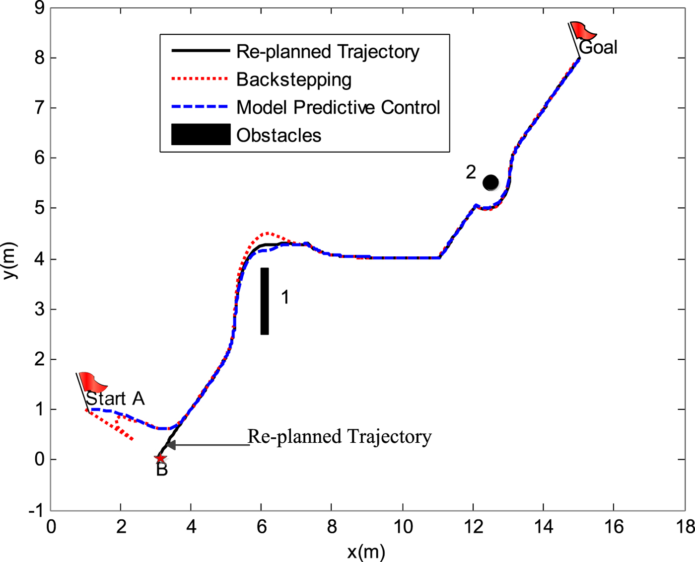
Figure 13. Re-planned trajectory tracking control.

The red dotted line represents backstepping tracking results, and the blue dotted line represents the MPC tracking results, while the black solid line represents the reference trajectory (re-planned trajectory). It can be seen from Figure 13 that these two methods overcome the same initial trajectory error. After the AUV reaches the desired trajectory and begins to track stably, the three lines almost coincide. This means the tracking controllers based on both backstepping and MPC methods successfully make the AUV track the trajectory as desired.

As introduced before, Figure 13 is a simulation result and the control is thought to be realised unconditionally. Due to the real-world AUV constraints, the control data produced by the backstepping method is difficult to realise. Thus, in reality, the backstepping controller cannot track a re-planned trajectory such as the result shown in Figure 13.

In this part, the maximum velocity of the AUV is 3 m/s, and the minimum is −3 m/s. Only a normalised velocity value in the range of [−1, 1] is acceptable for the AUV. The normalised velocity curve and speed jump of these two controllers are shown in Figures 14 and 15, and it is obvious that the two normalised velocity lines almost coincide as time progresses. However, at the beginning, in Figure 14, the velocity values of the backstepping algorithm changes quickly. Table 3 shows the normalised velocity of points C and D, corresponding to times 0·05 s and 0·1 s, and the time interval between them is 0·05 s (a sampling step).

Figure 14. Comparison of normalised velocity.

Figure 15. Comparison of normalised speed jump.

Table 3. The normalised velocity comparison of polyline tracking

The MPC controller considers the speed constraints of the AUV, so at points C and D in Table 3, it can be seen that all normalised velocities of the MPC controller are in the range [−1, 1] and the sign of the velocity stays steady over this small time step. However from C to D, the linear velocity u of the backstepping algorithm changes from a positive value 3·65 to a negative value −2·61, v changes from −9·32 to 2·33 and yawing speed r changes from −3·86 to 2·20. It is clear that u, v and r are outside the range [−1, 1]. Also, in a sampling step, the sign changes too quickly and the speed jump is sharp. In real conditions, as mentioned before, because of the constraints of the AUV, a big speed jump is difficult to achieve and the fast sign change should be avoided.

Since the polyline is not a continuous trajectory, it is not differentiable at the turning point. The main problem of trajectory tracking is the speed jump caused by the initial position and the error of the turning point position. Table 4 shows the maximum normalised speed jump of the AUV at the beginning, the obstacle positions and the turning point. At the beginning, for the backstepping algorithm, the linear speed jump Δ u _c and Δ v _c are $-6\cdot26<-1$ and 11·64 > 1, the yawing speed jump is 6·60 > 1, and they all exceed the limit [−1, 1]. The normalised value of the linear and yawing velocities of the MPC algorithm at the beginning are small and all inside the limit [−1, 1]. At the turning point, the main speed jump is caused by the angular velocity and the linear speed jump is not obvious. So here, the angular speed jump is the focus. Points E and F in Figure 15 represent the angular speed jump of the backstepping method (with enlarged view in Figure 16). The normalised value at points E and F are −0·6 and 0·6, which are shown in Table 4. At the same place, the angular speed jumps of the MPC controller are 0·04 and −0·032. The speed jump of backstepping control is almost 15 times bigger than the MPC control method. When the AUV encounters the obstacles, the maximum speed jump is in the acceptable range [−1, 1], which means that with this method trajectory tracking and avoidance motion can be realised.

Figure 16. Enlarged view of angular speed jump.

Table 4. The maximum normalised speed jump of polyline tracking

Figure 17 shows the calculation times per controller step in polyline trajectory tracking. Similar to the computation time analysis of circle tracking mentioned above, if there is an obstacle in range or the vehicle is away from the desired trajectory, the computation time per controller step increases, and most of the controller processing is completed within one controller time step, showing that the proposed method is suitable for online application. Notice that computation time is presented here for reference purposes only, because these time measurements are highly variable depending on factors such as the processor speed and programming environment.

Figure 17. Computation time per controller step.

As introduced in Section 4.1, sharp speed jumps and fast sign changes will not work in reality. So, the backstepping method cannot track a re-planned trajectory such as in our simulation results. The MPC algorithm, because of its own constraints, is more achievable in real life.

From the two simulation results above, it can be seen that the MPC re-planning method can successfully plan a trajectory to avoid the obstacles. Model predictive control can accomplish a certain function in meeting the constraint conditions, and the trajectory tracking based on MPC can help the AUV solve the speed jump problem effectively compared to the trajectory tracking of the backstepping algorithm.