


NOMENCLATURE
- A i
weighting coefficient of shape function
- a n
coefficient of basis function
- C(ψ)
class function
- c
chord length
- K i
binomial coefficient
- n
order of Bernstein polynomials
- p, q
control parameters of leading-edge basis function
- R le
leading-edge radius
- S(ψ)
shape function
- z(x)baseline
co-ordinate of base aerofoil
- z error
typical wind tunnel tolerance
- z i,original(ψ)
co-ordinate of original aerofoil
- z i,fitting(ψ)
co-ordinate of fitting aerofoil
- α, β
control parameters of trailing-edge basis function
- ψ
non-dimensional co-ordinate in chordwise
- ζ T
trailing-edge thickness ratio in class/shape function transformation
- θ
trailing-edge angle
- Δz te
trailing-edge thickness
- ϕ n (ψ)
basis function
1.0 INTRODUCTION
Aerofoil shape parameterisation, using a mathematical representation to represent the aerofoil geometry, is a principal step in aerodynamic optimisation. Because different design variables can generate different aerofoils, so shape parameterisation can directly affect the design space of aerofoils. Moreover, the more precise the aerofoil geometry is, the higher the accuracy of the aerofoil aerodynamic design is. Therefore, it is very important for the aerofoil designers to select a suitable shape parameterisation method for the aerofoil optimisation design.
A wide range of methods have been previously used for aerofoil geometry representation. Castonguay and Nadarajah( Reference Castonguay and Nadarajah 1 ) compared four parameterisation methods: the mesh points, B-spline, Hicks–Henne bump function and PARSEC methods, in the aerofoil aerodynamic design. Five aerofoil parameterisation techniques, Ferguson’s curves, Hicks–Henne bump functions, B-splines, PARSEC and class shape functions transformation, were ranked according to the economy, intuitiveness, orthogonality, completeness and flawlessness by Sripawadkul( Reference Sripawadkul and Padulo 2 ). Master( Reference Masters, Taylor and Rendall 3 ) analysed seven parameterisation methods: class shape transformations, B-splines, Hicks–Henne bump functions, a radial basis function domain element approach, Bezier surfaces, a singular-value decomposition modal extraction method and the parameterised sections method, and tested the efficiency of these parameterisation methods.
Kulfan( Reference Kulfan 4 ) proposed that the geometric representation should have the following properties: (1) well behaved and produces smooth and realistic shapes; (2) few design variables to represent the whole aerofoil; (3) high flexibility to cover the optimum aerodynamic shapes; (4) intuitiveness of design variables. And Kulfan( Reference Kulfan and Bussoletti 5 ) developed the class shape function transformation (CST) parameterisation method to represent the aerofoils. The CST method, which possesses the above properties, is widely used in the aerofoil aerodynamic optimisation design( Reference Kulfan 4 – Reference Vu and Lee 8 ). In the CST the leading-edge radius, the closure boat-tail angle and trailing-edge thickness are the intuitive control parameters. However, it is very difficult to set the leading-edge radius and the leading-edge radius of the upper aerofoil and the lower aerofoil are different for most aerofoils. Moreover, the ability of the Bernstein polynomial to control the leading-edge is not good. Therefore, Kulfan( Reference Kulfan 9 ) proposed the leading-edge modification (LEM) to the CST method. Although this modification increases an additional basis function, the precision of representing the aerofoil is improved and the number of control parameters significantly reduces.
The Hicks–Henne bump function’s( Reference Hicks and Henne 10 ) method was proposed to represent the aerofoil. Hicks–Henne bump functions could capture all aerofoil features with the highest number of design variables( Reference Sripawadkul and Padulo 2 ). The greater the number of the design variables is, the lower the efficiency of the aerofoil optimisation becomes for the same optimisation algorithm. Moreover, the ability of bump functions to control the trailing edge is bad and the shape of the trailing edge remains almost unchanged. So the improved Hicks–Henne bump function’s method( Reference Chen, Guo and Yi 11 , Reference Liang, Meng and Tong 12 ) was used to optimise the aerofoils. And the improved Hicks–Henne bump function’s method indeed expands the aerofoil design space.
For some large camber and complex aerofoils, the fitting precision of the LEM CST near the trailing edge is limited and the ability to adjust the leading edge is also limited. Since the LEM CST method can reach relatively high flexibility with a reasonably few number of design variables and the improved Hicks–Henne bump function’s method can spread the trailing edge, so a new CST method is proposed to parameterise the aerofoil by combining the LEM CST method with the improved Hicks–Henne bump function’s method. The key of the NEW CST method is to confirm the leading-edge basis function and trailing-edge basis function. So the Genetic Algorithm (GA)( Reference Goldberg 13 ) is proposed to gain the parameters of the basis functions. Some samples are generated by the Latin hypercube design (LHD) method( Reference Mackay, Beckman and Conover 14 ) and the radial basis functions neural network (RBF) model( Reference Kharal and Saleem 15 ) is trained by these samples. The NEW CST method is proved to be better than the LEM CST method and the parameterisation performance of the NEW CST method in fitting a series of aerofoils is accessed by comparison with the LEM CST method and the original CST method.
2.0 SHAPE PARAMETERISATION
2.1 Class-function/shape-function transformations
Kulfan( Reference Kulfan 4 ) and Kulfan and Bussoletti( Reference Kulfan and Bussoletti 5 ) developed the CST method to represent aerofoils with relatively few control parameters. This method is widely used in aerofoil optimisation. The aerofoil is defined as
 $${z \over c}{\equals}\sqrt {{x \over c}} \cdot \left( {1{\minus}{x \over c}} \right) \cdot \mathop{\sum}\limits_{i{\equals}0}^N {\left[ {A_{i} \cdot \left( {{x \over c}} \right)^{i} } \right]{\plus}{x \over c} \cdot {{\Delta z_{{te}} } \over c}} $$
This form can be rewritten as
 $$\zeta ({\rm \rpsi }){\equals}C({\rm \rpsi })S({\rm \rpsi }){\plus}{\rm \rpsi \zeta }_{T} ,$$
where
 $${\rm \rpsi }{\equals}x/c$$
,
$${\rm \rpsi }{\equals}x/c$$
,
 $${\rm \xi }{\equals}z/c$$
,
$${\rm \xi }{\equals}z/c$$
,
 $${\rm \xi }_{T} {\equals}\Delta {\rm \xi }_{{{\rm TE}}}/c$$
, C(ψ) is the class function and S(ψ) is the shape function
$${\rm \xi }_{T} {\equals}\Delta {\rm \xi }_{{{\rm TE}}}/c$$
, C(ψ) is the class function and S(ψ) is the shape function
 $$C({\rm \rpsi }){\equals}({\rm \rpsi })^{a} (1{\minus}{\rm \rpsi })^{b} $$
 $$S({\rm \rpsi }){\equals}{{{\rm \xi }({\rm \rpsi }){\minus}{\rm \rpsi \xi }_{T} } \over {\sqrt {\rm \rpsi } (1{\minus}{\rm \rpsi })}}{\equals}\mathop{\sum}\limits_{i{\equals}0}^n {A_{i} BP_{{i,n}} ({\rm \rpsi })} $$
The class parameters a and b for the general aerofoil with a round nose and an aft end trailing edge are set to 0.5 and 1.0. The Bernstein polynomial is employed as the shape function to describe the detailed shape as
 $$BP_{{i,n}} ({\rm \rpsi }){\equals}K_{i} {\rm \rpsi }^{i} (1{\minus}{\rm \rpsi })^{{n{\minus}i}} ,$$
where K i is the binomial coefficient and n is the order of the Bernstein polynomial.
Kulfan( Reference Kulfan 9 ) presented a leading-edge modification (LEM) to the CST method, adding an extra basis function, to improve the flexibility of the CST method. The LEM CST is as follows:
 $$S({\rm \rpsi }){\equals}\mathop{\sum}\limits_{i{\equals}0}^n {A_{i} BP_{{i,n}} ({\rm \rpsi })} {\plus}A_{{n{\plus}1}} {\rm \rpsi }^{{0.5}} (1{\minus}{\rm \rpsi })^{{n{\minus}0.5}} $$
This LEM CST method was proved to be effective and could improve the precision of the aerofoil fitting( Reference Kulfan 9 ).
2.2 Improved Hicks–Henne bump function
Hicks and Henne( Reference Hicks and Henne 10 ) proposed to use bump functions for aerofoil design. The aerofoil shape can be represented by the following equations:
 $$z({\rm \rpsi }){\equals}z({\rm \rpsi })_{{\rm baseline}} {\plus}\mathop{\sum}\limits_{n{\equals}1}^N {a_{n} {\rm \rvarphi }_{n} ({\rm \rpsi })} ,$$
where
 $$z({\rm \rpsi })_{{\rm baseline}} $$
is the co-ordinate of the base aerofoil. ϕ
n
(ψ) is the basis function and a
n
is the coefficient:
$$z({\rm \rpsi })_{{\rm baseline}} $$
is the co-ordinate of the base aerofoil. ϕ
n
(ψ) is the basis function and a
n
is the coefficient:
 $$\eqalignno{ & {\rm \rvarphi }_{1} ({\rm \rpsi }){\equals}{\rm \rpsi }^{{0.25}} (1{\minus}{\rm \rpsi })e^{{{\minus}20\rpsi }} \cr & {\rm \rvarphi }_{n} ({\rm \rpsi }){\equals}\sin ^{3} ({\rm \rpi \rpsi }^{{\log 0.5/\log x_{n} }} )\matrix{ {} & {0\leq x_{n} \leq 1} \cr } $$
Because the basis function and its derivative are both 0 at ψ=1, so the variation at the trailing edge is also 0. It leads that the new aerofoils have no change in comparison with the original aerofoil near the trailing edge. It is disadvantageous for the optimisation of the aerofoil. Therefore, a new basis function is added near the trailing edge. The improved Hicks–Henne function is as follows:
 $${\rm \rvarphi }_{n} ({\rm \rpsi }){\equals}\left\{ \matrix{ {\rm \rpsi }^{{0.25}} (1{\minus}{\rm \rpsi })e^{{{\minus}20\rpsi }} \matrix{ {\matrix{ {\matrix{ {} & {} \cr } } & {} \cr } } & {n{\equals}1} \cr } \hfill \cr \sin ^{3} ({\rm \rpi \rpsi }^{{\log 0.5/\log x_{n} }} )\matrix{ {} & {} & {2\leq n\leq N{\minus}1} \cr } \hfill \cr {\rm \ralpha \rpsi }(1{\minus}{\rm \rpsi })e^{{{\minus}\rbeta (1{\minus}\rpsi )}} \matrix{ {} & {} & {} & {n{\equals}N,} \cr } \hfill \cr} \right.$$
where α and β are the control parameters of the basis function. α can control the slope of the basis function and β can control the attenuation of the basis function.
The derivative of the improved Hick–Henne basis function is not 0 at ψ = 1. The representation of aerofoil on the trailing edge is improved and the design space of the aerofoil is expanded by the improved Hicks–Henne basis function( Reference Chen, Guo and Yi 11 , Reference Liang, Meng and Tong 12 ).
2.3 Combination of CST and Hicks–Henne bump function: new CST method
Kulfan and Bussoletti( Reference Kulfan and Bussoletti 5 ) and Ceze et al.( Reference Ceze, Hayashi and Volpe 16 ) expounded that the CST method could represent most aerofoils with high accuracy when the Bernstein polynomial order is higher than 9. But for some large camber and complex aerofoils such as S1223, E216 and NLR7301, the high order Bernstein polynomial cannot reach the accuracy requirement of these aerofoils. Moreover, the representation on the aerofoil at the leading edge and trailing edge is bad and the fitting error is large. So, Kulfan( Reference Kulfan 9 ) proposed the leading-edge modification (LEM) to the CST method. Though the LEM CST method adds a control parameter in comparison with the original CST method, it improves the geometric accuracy for aerofoils and also reduces the order of the Bernstein polynomial( Reference Masters, Taylor and Rendall 3 , Reference Masters, Poole and Taylor 17 ).
Five properties including completeness, orthogonality, flawlessness, economy and intuitiveness( Reference Sripawadkul and Padulo 2 , 18 ) are specified to evaluate the merits and demerits of the aerofoil parameterisation. In the RAE2822 aerofoil fitting( Reference Sripawadkul and Padulo 2 ), 32 design variables were required to reach the typical wind tunnel tolerance using the Hicks–Henne bump function. It indicates that the economy of the Hicks–Henne bump function is worse than the other fitting methods. And the Hicks–Henne bump function method is non-orthogonal in comparison with the CST method. Moreover, the capacity of the Hicks–Henne bump function method to represent the aerofoil trailing edge is limited( Reference Chen, Guo and Yi 11 , Reference Liang, Meng and Tong 12 ). As mentioned before, the modified Hicks–Henne bump function can improve the fitting precision of the aerofoil trailing edge.
When we use the LEM CST method and the original CST to parameterise the aerofoils, we find that the fitting errors near the trailing edge are large especially for some highly cambered trailing-edge aerofoils. In section Improved Hicks–Henne bump function, the improved Hick–Henne bump function( Reference Chen, Guo and Yi 11 , Reference Liang, Meng and Tong 12 ) can offer the more flexible expression form on the trailing edge and expand the design space of the aerofoil. And the higher fitting precision near the trailing edge can be obtained. So the trailing-edge base function of the improved Hick–Henne bump function is combined with the original CST method to improve the fitting precision.
The essence of the aerofoil parameterisation is that different basis functions are superposed together to approach the original aerofoil. Moreover, these different basis functions can produce different fitting errors and we need to choose suitable basis functions to obtain the smallest fitting error. It is effective for the LEM CST method( Reference Kulfan 9 ) to parameterise the large nose camber aerofoils and it can reduce the number of terms by comparison with the original CST. To accommodate different nose camber aerofoils, the leading-edge basis function of the LEM CST is improved. Because Equation (9) can generate different basis functions for the different x n and completely include Kulfan’s LEM basis function in Fig. 2, so the second item of Equation (9) is used as the new leading-edge modification basis function.
In this paper, the new leading-edge modification basis function and the trailing edge basis function are combined to parameterise the aerofoil. The LEM CST method is improved by introducing the parameter p to control the leading edge of the aerofoil. Different basis functions are obtained by changing p. The fitting ability to the leading edge is better than the LEM CST. The parameter q can control the amplitude of the basis function. And the trailing-edge modification function (TEM) is introduced into the NEW CST method. α and β are the control parameters of the trailing-edge basis function. α can control the amplitude of the basis function. Different β can produce different basis functions. So it can improve the fitting precision of the trailing edge. The NEW CST is as follows:
 $$\eqalignno{ {\rm \zeta }({\rm \rpsi }){\equals}C({\rm \rpsi })\mathop{\sum}\limits_{i{\equals}0}^n {A_{i} BP_{{i,n}} ({\rm \rpsi })} {\plus}\mathop{\underbrace{{A_{{n{\plus}1}} \cdot {\rm \ralpha } \cdot {\rm \rpsi }(1{\minus}{\rm \rpsi })e^{{{\minus}{\rm \rbeta }(1{\minus}{\rm \rpsi })}} }}}\limits_{\rm TEM}{\plus} \cr \mathop{\underbrace{{A_{{n{\plus}2}} \cdot q \cdot \sin ^{3} ({\rm \rpi \rpsi }^{{\log (0.5)/\log (p)}} )}}}\limits_{\rm LEM}{\plus}{\rm \rpsi \zeta }_{T}&$$
Equation (10) can be written as
 $${\rm \zeta }({\rm \rpsi }){\equals}C({\rm \rpsi })\mathop{\sum}\limits_{i{\equals}0}^n {A_{i} BP_{{i,n}} ({\rm \rpsi })} {\plus}\mathop{\underbrace{{A_{{n{\plus}1}} {\rm \rpsi }(1{\minus}{\rm \rpsi })e^{{{\minus}{\rm \rbeta }(1{\minus}{\rm \rpsi })}} }}}\limits_{\rm TEM}{\plus}\mathop{\underbrace{{A_{{n{\plus}2}} \sin ^{3} ({\rm \rpi \rpsi }^{{\log (0.5)/\log (p)}} )}}}\limits_{\rm LEM}{\plus}{\rm \rpsi \zeta }_{T} $$
The weight coefficients A n and A n+1 are corresponding to the trailing-edge angle and trailing-edge vertical position:
 $$S(1){\equals}A_{n} {\equals}\tan (\theta ){\minus}A_{{n{\plus}1}} {\plus}{{\Delta z_{{te}} } \over c}$$
 $$A_{n} {\plus}A_{{n{\plus}1}} {\equals}\tan (\theta ){\plus}{{\Delta z_{{te}} } \over c}$$
The design variables of the NEW CST method are the weight coefficients A i (i=0,1,…,n+2) in Equation (11). The NEW CST method has two additional basis functions in comparison with the original CST. And the LEM CST method has one additional basis function in contrast with the original CST. The number of design variables is BPONEW+3 (BPO is the order of Bernstein polynomial) and the numbers of design variables for the LEM CST and the original CST is listed in Table 1. The NEW CST introduces two parameters (p and β) to control the additional basis functions. There are different basis functions for different aerofoils using the NEW CST method.
Table 1 Design variables of the original CST, LEM CST and NEW CST

The basis functions for the six design variables CST configuration are shown in Fig. 1. The red dashed lines represent the basis functions for the original CST method. The blue dotted lines represent the basis functions for the aerofoil leading-edge and the black solid lines are the basis functions for the aerofoil trailing-edge. Different p (p=0.01, p=0.1, p=0.5) can generate different basic functions in Fig. 1. If p is larger, the ability to control the leading-edge is worse. Because the basis function is more flat near the leading edge and the value of the basis function at ψ = 0 is close to 0. If p is smaller, the ability to control the leading-edge is also worse. Because the basis function is steeper near the leading edge and the value of the basis function at ψ = 0 is close to the constant (0.3), so it is necessary to choose the appropriate p to obtain the leading-edge modification basis function. When 0.13≤ p ≤0.3, NEW LEM basis functions can completely include Kulfan’s LEM basis function in Fig. 2. So the NEW CST method can generate more aerofoils. In Fig. 1, different β (β=5, β=20, β=50) can generate different trailing-edge modification basis functions. When β (β=50) is larger, the trailing-edge modification (TEM) basis function quickly decays. And this leads the ability of TEM basis function to control the aerofoil trailing-edge declines and makes the fitting aerofoil distorted. When β (β=5) is smaller, the TEM basis function has an influence on the original CST basis function. Therefore, β is an important parameter to control the aerofoil trailing-edge.
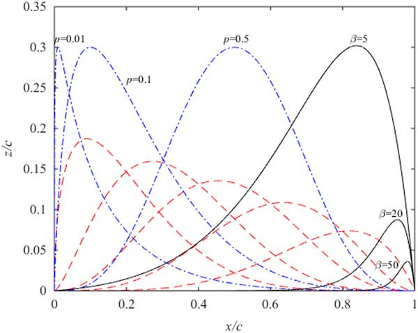
Figure 1 Basis functions of the NEW CST.
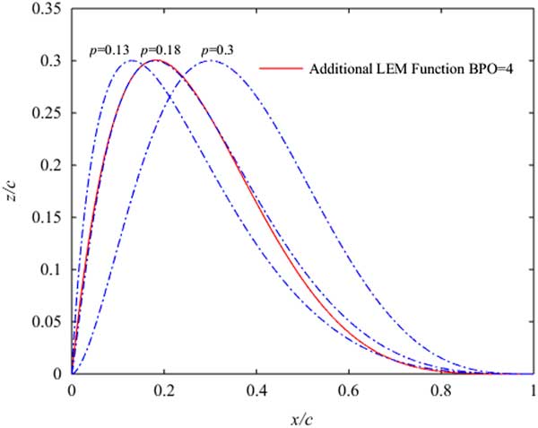
Figure 2 Basis functions at the leading edge.
The derivatives of the TEM basis functions (β=2, β=5, β=15, β=100) are represented in Fig. 3. If the derivative of the TEM basis function is not 0, it indicates that the TEM basis function is not constant. In the figure, when β (β=2) is smaller, the derivative of the aerofoil middle co-ordinate is larger than 0. It indicates that the TEM basis function can affect the aerofoil middle co-ordinate. Furthermore, the smaller β is, the greater the sphere of influence to the aerofoil middle co-ordinate. When β (β=100) is larger, though the TEM basis function has no effect on the LEM basis function and original CST basis function, the variation of the TEM basis function becomes greater. The ability to manipulate the aerofoil trailing-edge is poor. So we should choose a suitable TEM function.

Figure 3 Derivatives of trailing edge modification basis functions.
3.0 GEOMETRIC INVERSE FITTING TEST AND RESULTS
A well-behaved parameterisation method should be able to represent a wide range of existing aerofoils with high accuracy. It is necessary to test the aerofoil shape recoverability. So the University of Illinois Urbana Champaign (UIUC) aerofoil database (see footnote Footnote *) is applied to test the new parameterisation method and there are about 1,550 kinds of aerofoils in this database. To accommodate the proposed NEW CST, the original CST and the LEM CST methods, the geometries of all the aerofoils are normalised. So an impartial and consistent testing platform can be provided in this paper. The aerofoil normalisation is detailed in Appendix A.
3.1 Geometric inverse fitting error
A statistics method is employed to access the fitting errors. The root mean square error (RMSE)( Reference Willmott 19 ) has been used as a standard statistical metric to measure the NEW CST method. The RMSE is as follows:
 $${\rm RMSE}{\equals}\sqrt {{1 \over n}\mathop{\sum}\limits_{i{\equals}1}^n {(z^{{i,{\rm fitting}}} (\rpsi ){\minus}z^{{i,{\rm original}}} (\rpsi ))^{2} } } $$
where
 $$z^{{i,{\rm original}}} ({\rm \rpsi })$$
is the co-ordinate of the original aerofoil and
$$z^{{i,{\rm original}}} ({\rm \rpsi })$$
is the co-ordinate of the original aerofoil and
 $$z^{{i,{\rm fitting}}} ({\rm \rpsi })$$
is the co-ordinate of the fitting aerofoil. n is the number of the upper or lower aerofoil co-ordinate.
$$z^{{i,{\rm fitting}}} ({\rm \rpsi })$$
is the co-ordinate of the fitting aerofoil. n is the number of the upper or lower aerofoil co-ordinate.
In the NEW CST method, different p and β can produce different leading-edge basis functions and trailing-edge basis functions and the RMSE of this method is also different. When n is constant, the minimum RMSE is obtained by choosing the suitable leading-edge and trailing-edge basis functions. So p and β should be calculated first and the leading-edge and trailing-edge basis functions of the NEW CST method can be determined. The sensitivity of the RMSE to the parameters p and β is researched. The S1223 aerofoil is used to measure the feasibility and accuracy of the NEW CST. When the number of control parameters (NCP) for the NEW CST is equal to the LEM CST, different p and β are discussed. The NCP of these two methods for the S1223 aerofoil is 15. The RMSE of the S1223 upper aerofoil for the LEM CST is 1.3637×10⁻⁴ and the lower aerofoil is 7.7261×10⁻⁵. When 0<p<0.2, different β (β=20, β=50, β=100) of the NEW CST method are analysed. When 0<β<300 of the upper aerofoil and 0<β<100 of the lower aerofoil, p=0.015, p=0.02, p=0.035 of the upper aerofoil and p=0.015, p=0.02, p=0.025, p=0.08, p=0.1 of the lower aerofoil are analysed using the NEW CST method. The RMSE results of the S1223 aerofoil are shown in Figs 4 and 5.

Figure 4 RMSE of the S1223 upper aerofoil.

Figure 5 RMSE of the S1223 lower aerofoil.
In Fig. 4. as p ranges from 0 to 0.04 for the upper aerofoil of S1223, the RMSE has a trough and the smallest RMSE is 6.736×10⁻⁵. And when p ranges from 0.04 to 0.2, the upper aerofoil has also the smallest RMSE: 6.7465×10⁻⁵. Moreover, when β changes from 0 to 300, the RMSE has the trough and it is 4.1581×10⁻⁵ (p=0.015, β=180). In Fig. 5, as p ranges from 0 to 0.2 for the lower aerofoil of S1223, the RMSE has two troughs and they are 3.5394×10⁻⁵ (p=0.015, β=20) and 3.0859×10⁻⁵ (p=0.08, β=20). When 0<β<100, the lower aerofoil has the smallest RMSE. So the suitable p and β of the NEW CST can be obtained by comparison with the RMSE of the LEM CST.
3.2 Confirming the basis functions of NEW CST method
The relationship among p, β and RMSE is complicated and non-linear. In order to obtain the suitable leading-edge and trailing-edge basis functions, p and β are sampled by the Latin hypercube design (LHD) method and the radial basis functions neural network (RBF) model is trained by the sample data. So the approximation relationship among p, β and RMSE can be obtained. MATLAB’s Genetic Algorithm (GA) toolbox has been used to acquire the minimum RMSE and the optimisation process is represented in Fig. 6.

Figure 6 Optimisation process of the NEW CST method.
There are three assessments to validate the accuracy of the RBF model: the root mean square error (RMSERBF), the maximum absolute error (MAX) and the correlation coefficient (R 2)( Reference Li, Gao and Gu 20 ). RMSERBF is used to measure the global accuracy of the RBF model; MAX is employed to evaluate the local accuracy of the RBF model; R 2 can reflect the linear dependence between the predicted values of the RBF model and the actual values. When RMSERBF=0, MAX=0, and R 2=1, the RBF model goes through these samples. So the closer RMSERBF is to 0, MAX is to 0, and R 2 is to 1, the higher the prediction precision of the RBF model is. NASA_SC20714, FX63_137 and S1223 aerofoils are used to confirm the basis functions. 500 samples are generated by using the LHD method for each aerofoil and these samples are approached by the RBF model. These samples are shown in Figs 7–12 and the results of the RBF model are listed in Table 2. Parameter settings of the GA optimisation are as follows: the sub-population size is 10, the number of island is 10, the number of generations is 10, the rate of crossover is 0.95, the rate of mutation is 0.01, the rate of migration is 0.3 and the interval of migration is 4. The optimisation results are represented in Table 2. So we can use the suitable basis functions to fit the aerofoils and obtain the minimum RMSECST.

Figure 7 RMSE of the NASA_SC20714 upper aerofoil.

Figure 8 RMSE of the NASA_SC20714 lower aerofoil.

Figure 9 RMSE of the FX63_137 upper aerofoil.
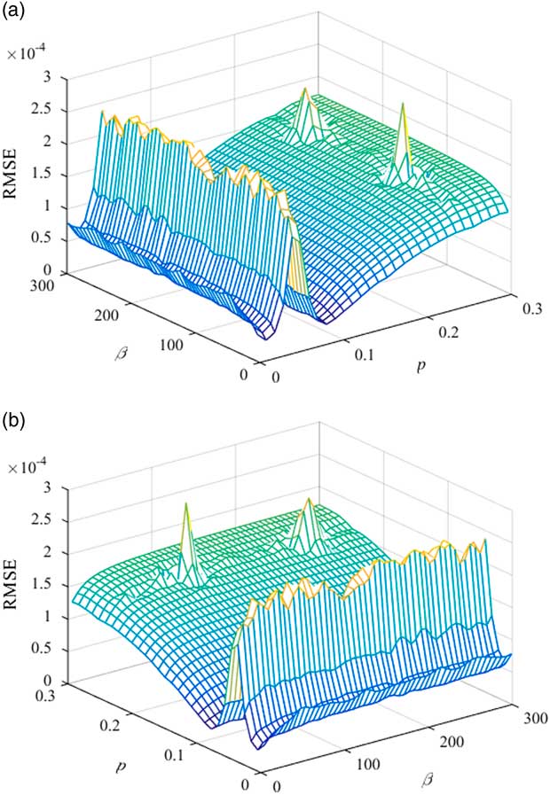
Figure 10 RMSE of the FX63_137 lower aerofoil.

Figure 11 RMSE of the S1223 upper aerofoil.

Figure 12 RMSE of the S1223 lower aerofoil.
Table 2 GA optimisation results

The results of RMSERBF and R 2 can reach the requirement of the RBF approximation model from Table 2, when 500 samples are generated by the LHD method. The NEW CST for the S1223 aerofoil is as follows:
 $${\rm \zeta }_{{{\rm Upper}}} ({\rm \rpsi }){\equals}C({\rm \rpsi })\mathop{\sum}\limits_{i{\equals}0}^{12} {A_{i} BP_{{i,12}} ({\rm \rpsi })} {\plus}A_{{13}} \cdot {\rm \rpsi }(1{\minus}{\rm \rpsi })e^{{{\minus}168.66(1{\minus}{\rm \rpsi })}} {\plus}A_{{14}} \cdot \sin ^{3} (\rpi {\rm \rpsi }^{{\log (0.5)\,/\,\log (0.07717)}} ){\plus}{\rm \rpsi \zeta }_{T} $$
 $${\rm \zeta }_{{{\rm Lower}}} ({\rm \rpsi }){\equals}C({\rm \rpsi })\mathop{\sum}\limits_{i{\equals}0}^{12} {A_{i} BP_{{i,12}} ({\rm \rpsi })} {\plus}A_{{13}} \cdot {\rm \rpsi }(1{\minus}{\rm \rpsi })e^{{{\minus}17.56(1{\minus}{\rm \rpsi })}} {\plus}A_{{14}} \cdot \sin ^{3} ({\rm \rpi \rpsi }^{{\log (0.5)\,/\,\log (0.08515)}} ){\plus}{\rm \rpsi \zeta }_{T} $$
3.3 Tested on UIUC aerofoil database
The University of Illinois Urbana Champaign (UIUC) aerofoil database consists of about 1,550 kinds of aerofoils. The UIUC aerofoil database is tested to validate the improved capability of the new parameterisation by comparison with the LEM CST and the original CST. In general, [0,0] is the leading edge point and [1,0] is the trailing edge point. To make it easier to compare these three methods, all the aerofoils have been normalised to ensure
 $$0\leq \rpsi \leq 1$$
.
$$0\leq \rpsi \leq 1$$
.
The root mean square error (RMSE) has been used as a standard statistical metric to compare these three methods. When the number of the weight coefficients A
n
is the same, the RMSEs of these three methods are calculated and obtained. Two situations (BPO=4 and BPO=7) are analysed and 1,545 aerofoils are tested. In general, the smaller the value of RMSE is, the higher the fitting precision is. The RMSE is converted to the logarithmic for ease of comparison and the logarithmic expression is
 $$Q{\equals}{\minus}\log _{{10}} (RMSE)$$
. So we need to compare the size of Q. The results of the upper aerofoils and the lower aerofoils are presented in Figs 13 and 14 (the black solid line represents the NEW CST, the red dashed line represents the LEM CST and the blue dotted line represents the original CST). The aerofoil number 1–100, number 400–500, number 900–1000 and number 1,400–1,500 of the UIUC library are clearly shown in Figs 13 and 14.
$$Q{\equals}{\minus}\log _{{10}} (RMSE)$$
. So we need to compare the size of Q. The results of the upper aerofoils and the lower aerofoils are presented in Figs 13 and 14 (the black solid line represents the NEW CST, the red dashed line represents the LEM CST and the blue dotted line represents the original CST). The aerofoil number 1–100, number 400–500, number 900–1000 and number 1,400–1,500 of the UIUC library are clearly shown in Figs 13 and 14.
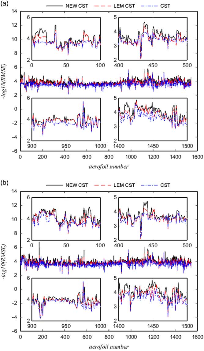
Figure 13 RMSE results of BPO=4 for the NEW CST, the LEM CST and the original CST when tested on the UIUC library. (a) RMSE results of the upper aerofoil and (b) RMSE results of the lower aerofoil.
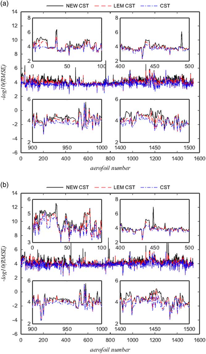
Figure 14 RMSE results of BPO=7 for the NEW CST, the LEM CST and the original CST when tested on the UIUC library. (a) RMSE results of the upper aerofoil and (b) RMSE results of the lower aerofoil.
In Fig. 13, when BPO=4, the NEW CST methods is more accurate than the LEM CST and the fitting accuracy of the LEM CST is higher than the original CST. In the NEW CST method, 92.36% of the UIUC library are superior to the LEM CST for the RMSE of the upper aerofoil and 94.56% are superior to the original CST. The remaining 7.64% of the UIUC library using the NEW CST are close to the LEM CST and 5.44% of aerofoils approach to the original CST. For the RMSE of the lower aerofoil, about 91.13% of the UIUC library are superior to the LEM CST and 92.69% of the UIUC library precede the original CST.
In Fig. 14, when BPO=7, the NEW CST method is obviously superior to the LEM CST and the fitting precision is the highest among these three methods. About 89.9% of the UIUC library for the RMSE of the upper aerofoil are superior to the LEM CST and 91.2% are superior to the original CST. At the same time, 93.53% of the UIUC library for the RMSE of the lower aerofoil precede the LEM CST and 91.39% precede the original CST. The fitting precision of the remaining aerofoils for the NEW CST basically approaches to the LEM CST and the original CST.
3.4 Case studies on the leading edge and trailing edge
In section Geometric Inverse Fitting Test and Results, 1,545 aerofoils of the UIUC library are recovered by the NEW CST, the LEM CST and the original CST. When the number of control parameters is the same for these three methods, the NEW CST method has the highest fitting precision for the UIUC library. Because the NEW CST method has the better leading edge modification base function and trailing edge base function by comparison with the LEM CST and the original CST. So some complex aerofoils in the UIUC library are selected to further study the improved ability of the NEW CST at the leading edge and trailing edge.
In this section, a range of aerofoils, including high-lift low Reynolds number aerofoils (FX 63-137, S1223, E216)( Reference Selig and Guglielmo 21 ), supercritical aerofoils (NASA_SC20714, RAE2822, NLR7301)( Reference Zhu and Qin 22 , Reference Weber, Jones and Ekaterinaris 23 ), laminar aerofoils (NACA6412, NLF0416)( Reference Zhang, Fang and Chen 7 , Reference Kulfan 9 , Reference Hodge, Stone and Miller 24 ), sailplane aerofoils (AG16, E432)( Reference Hieu and Loc 25 , Reference Melin 26 ), and low-speed aerofoil (SA7035)( Reference Selig 27 ), have been employed to test the inverse fitting performance of the proposed NEW CST, the original CST and the LEM CST methods.
Kulfan and Bussoletti( Reference Kulfan 4 , Reference Kulfan and Bussoletti 5 ) defined a typical wind tunnel tolerance as the criterion of the geometric error. The typical wind tunnel tolerance is
 $$z^{{{\rm error}}} {\equals}\left\{ \matrix{ 3.5{\times}10^{{{\minus}4}} \matrix{ {} & {0\leq x/c\leq 0.2} \cr } \hfill \cr 7.0{\times}10^{{{\minus}4}} \matrix{ {} & {0.2\,\lt x/c\leq 1} \cr } \hfill \cr} \right.$$
z error are the errors between the approximated aerofoil and the original curves. In general, the fitting tolerance must reach the requirement of the typical wind tunnel test. If the error of the parameterised aerofoil is within the prescribed tolerance, the method is deemed successful. So this paper uses this tolerance to access the proposed NEW CST, the original CST, and the LEM CST methods.
Five types of aerofoils are applied to compare the fitting errors of the proposed NEW CST, the original CST and the LEM CST methods. The high-lift low Reynolds number aerofoils are employed for the first fitting test. The high-lift aerofoils have the larger camber around the trailing edge. They can increase payloads, shorten takeoff and landing distances, reduce aircraft noise, and lower stall speeds( Reference Selig and Guglielmo 21 ). FX63_137( Reference Foch and Ailinger 28 ) and E216 aerofoils are used in some small unmanned aerial vehicles. The S1223( Reference Ma, Zhong and Liu 29 ) aerofoil is applied to the design of the high altitude propeller. It is significant for the aircraft aerofoil design and optimisation to select the suitable method. The fitting aerofoils obtained by these three methods and the residual distributions are represented in Figs. 15–17. In Fig. 15, the first picture is the geometric fitting for FX63_137, the second picture shows the fewest numbers of the control parameters for these three methods when the geometric fitting errors can just reach the requirement of the typical wind tunnel tolerance, and the third picture is the geometric fitting error as the NCP is the same for these three methods.

Figure 15 Geometric fitting for FX63_137 using the original CST, LEM CST and NEW CST.
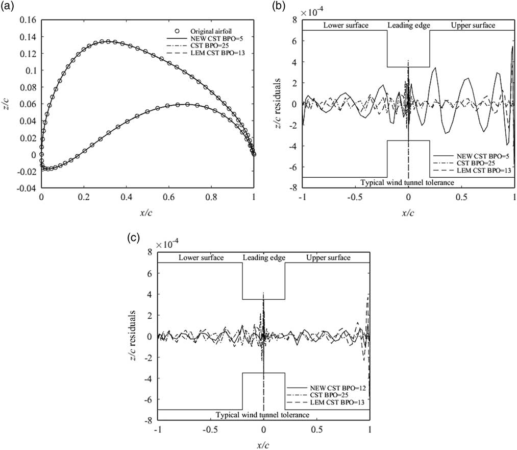
Figure 16 Geometric fitting for S1223 using the original CST, LEM CST and NEW CST.

Figure 17 Geometric fitting for E216 using the original CST, LEM CST and NEW CST.
The supercritical aerofoils, which are NASA_SC20714, RAE2822 and NLR7301, are accessed by these methods. The trailing-edge of the NASA_SC20714 aerofoil is open and this aerofoil is used in the PrandtlPlane( Reference Beccasio, Tesconi and Frediani 30 ). The RAE2822( Reference Wu, Mourrain and Galligo 31 ) aerofoil is widely applied in the high-speed subsonic aircraft. The NLR7301( Reference Zhang, Fang and Chen 7 ) aerofoil is a typical supercritical aerofoil with a large thickness. The fitting results of the proposed NEW CST, the original CST and the LEM CST methods are represented in Figs 18–20.

Figure 18 Geometric fitting for NASA_SC20714 using the original CST, LEM CST and NEW CST.

Figure 19 Geometric fitting for RAE2822 using the original CST, LEM CST and NEW CST.

Figure 20 Geometric fitting for NLR7301 using the original CST, LEM CST and NEW CST.
NACA6412 is the laminar flow 6-series aerofoil( Reference Abbott, Von Doenhoff and Stiver 32 ) developed by NACA and has small drag. NLF0416 is a low-speed natural laminar flow aerofoil. The NLF aerofoil is widely used in business jet designs. It can reduce the drag and improve the performance significantly( Reference Fujino, Yoshizaki and Kawamura 33 ). The fitting results of NACA6412 and NLF0416 aerofoils using these three methods are represented in Figs 21 and 22.

Figure 21 Geometric fitting for NACA6412 using the original CST, LEM CST and NEW CST.

Figure 22 Geometric fitting for NLF0416 using the original CST, LEM CST and NEW CST.
Sailplane aerofoils (AG 16, EPPLER432) and low-speed aerofoils (SA7035, SD8020) are tested by the proposed NEW CST, the original CST and the LEM CST methods. AG aerofoils were designed by Dr Mark Drela from MIT. SA aerofoils were improved from SD aerofoils( Reference Hieu and Loc 25 – Reference Selig 27 ). The test results are presented in Figs 23–25.

Figure 23 Geometric fitting for AG16 using the original CST, LEM CST and NEW CST.

Figure 24 Geometric fitting for EPPLER432 using the original CST, LEM CST and NEW CST.

Figure 25 Geometric fitting for SA7035 using the original CST, LEM CST and NEW CST.
As mentioned above, the proposed NEW CST method is composed of the original CST Bernstein polynomial, the leading-edge modification basis function, and the trailing-edge modification basis function. Therefore, two extra control parameters are added to the NEW CST method. And the LEM CST method has an additional control parameter compared to the original CST method.
FX 63-137, S1223 and E216 aerofoils have larger chamber and the complex leading edge and trailing edge. It leads that many more control parameters need to be used in the aerofoil fitting. The 15th-order CST (the number of control parameter (NCP) is 16) can reach the fitting precision of a typical wind tunnel test. And 8th-order LEM CST (NCP=10) can fit the FX63_137 aerofoil within the tolerance. When NCP is 9, the NEW CST can fit the FX63_137 aerofoil. When NCP is 10, the NEW CST has the higher precision than the LEM CST. Moreover, the tolerances of the leading-edge and trailing-edge are smaller than the LEM CST. The 25th-order CST of the S1223 aerofoil cannot reach the fitting precision of the typical wind tunnel test, especially at the location of the leading-edge and trailing-edge. And the LEM CST needs 15 control parameters. However, there are only eight control parameters to represent the S1223 aerofoil for the NEW CST method. When the number of control parameters for two methods is 15, the NEW CST method is more accurate than the LEM CST method by choosing the suitable p and β. The tolerances of the leading-edge and trailing-edge are smaller than the LEM CST. The 22th-order CST can fit the E216 aerofoil within the tolerance. And the NCP of the LEM CST is 14 and the NEW CST is 8. Moreover, when the NCP of the NEW CST is 11, it can reach the precision of the LEM CST.
For the supercritical aerofoils, the 10th-order CST can fit the NASA_SC20714 aerofoil within the errors of the typical wind tunnel. The RAE2822 aerofoil needs the 6th order and the NLR7301 aerofoil requires the 23rd order. For the laminar flow aerofoils, the 9th-order CST for the NACA6412 aerofoil can reach the precision requirement of the wind tunnel test. The NLF0416 aerofoil requires the 17th order. For the sailplane aerofoils and the low-speed aerofoils, the AG16 aerofoil needs the 10th-order CST, the EPPLER432 aerofoil needs the 22nd order and the SA7035 aerofoil requires the 12th order. The fitting results of the NEW CST and the LEM CST including the original CST are listed in Table 3.
Table 3 NCP of the original CST, LEM CST and NEW CST

The NEW CST can fit all test aerofoils to reach the typical wind tunnel tolerance. Moreover, the number of control parameters for the NEW CST is the fewest among these three methods. When the NCP of the NEW CST and LEM CST is the same, the RMSE of the NEW CST is smaller by adjusting p and β.
4.0 CONCLUSIONS
A new aerofoil parameterisation method is proposed by combining the leading edge modification CST method and improved Hicks–Henne bump functions method. Though the NEW CST method has two additional basis functions in comparison with the original CST, the fitting precision is better and the number of control parameters is fewer. Moreover, the number of control parameters of the NEW CST is fewer than the original CST for some complex aerofoils. The NEW CST introduces two parameters (p and β) to control the additional basis functions. Different p can generate different leading edge modification basis functions and the suitable β can reduce the representation errors of the trailing edge. Besides, the radial basis functions neural network model is trained by some samples (p, β and RMSE) which are generated by the Latin hypercube design (LHD) method. The relationship between p, β and RMSE can be obtained by the RBF model. And p and β are calculated by the Genetic Algorithm (GA) which can achieve the minimum RMSE of the NEW CST method. We can choose the suitable basis functions to fit the aerofoils. So the NEW CST method has an advantage over the LEM CST method in the aerofoil parameterisation.
The 1,545 UIUC aerofoils are tested to validate the improved capability of the new parameterisation by comparison with the LEM CST and the original CST. Furthermore, the leading-edge and trailing-edge fitting abilities of the NEW CST for high-lift low Reynolds number aerofoils, supercritical aerofoils, laminar aerofoils, sailplane aerofoils and low-speed aerofoil within the UIUC library are evaluated. The results show that the NEW CST can represent the whole aerofoils and the number of control parameters is the fewest among these three methods. Furthermore, when the NCP of the NEW CST and LEM CST is the same, the NEW CST method has a higher accuracy and smaller error especially at the leading edge and trailing edge.
The NEW CST method possesses the intuitive property like the original CST. Relatively few control parameters can represent the aerofoil and the fitting precision is high. Therefore, it is favorable for the aerofoil designers to select the NEW CST method to parameterise and optimise the aerofoil.
Appendix A. Aerofoil Normalisation
To make it easier to compare these three methods, all the aerofoils have been normalised to ensure that the leading-edge point is located at [0,0] and the trailing-edge point is located at [1,0]. We use the original data to normalise the aerofoil geometry. The normalisation factors of the upper and lower aerofoils are as follows:
 $$X_{{{\rm upper}}} {\equals}{{x_{{{\rm upper}}} {\minus}\min (x_{{{\rm upper}}} )} \over {\max (x_{{{\rm upper}}} ){\minus}\min (x_{{{\rm upper}}} )}}$$
 $$X_{{{\rm lower}}} {\equals}{{x_{{{\rm lower}}} {\minus}\min (x_{{{\rm lower}}} )} \over {\max (x_{{{\rm lower}}} ){\minus}\min (x_{{{\rm lower}}} )}}$$
Equations (A1) and (A2) can guarantee X upper, X lower∈[0, 1]. The co-ordinates of the leading-edge point and trailing-edge point are [x le,y le] and [x te,y te]. So the angle between the chord line and x-axis is
 $$\theta {\rm {\equals}arctan(}{{y_{{te}} {\minus}y_{{le}} } \over {x_{{te}} {\minus}x_{{le}} }})$$
The origin of the co-ordinate system is translated to the leading-edge point [x le,y le] by the co-ordinate translation. So the leading-edge point is located at [0,0]. According to the principle of the co-ordinate rotation, we can rotate x-y co-ordinate by θ degrees around [0,0]. So we can obtain the new x′–y′ co-ordinate and guarantee that the chord line is parallel to x′-axis
 $$\left[ \matrix{ {x'} \hfill \cr {y'} \hfill \cr} \right]{\equals}\left[ {\matrix{ {\cos \theta } & {\sin \theta } \cr {{\minus}\sin \theta } & {\cos \theta } \cr } } \right]\left[ \matrix{ x{\minus}x_{{le}} \hfill \cr y{\minus}y_{{le}} \hfill \cr} \right]$$
The rotation co-ordinate and scaling of the x′–y′ axes are shown in Figure A1. According to the normalisation equations (A1) and (A2), the x′–y′ scaling of the aerofoil can be obtained.

Figure A1 Rotation co-ordinate of the aerofoil.
 $$k_{{scale}} {\equals}{X \over {x\prime{\minus}{\rm min}\left( {x\prime} \right)}}{\equals}{1 \over {\max \left( {x\prime} \right){\minus}{\rm min}\left( {x\prime} \right)}}{\equals}{1 \over {{\raise0.7ex\hbox{${\left( {x_{{te}} {\minus}x_{{le}} } \right)}$} \!\mathord{\left/ {\vphantom {{\left( {x_{{te}} {\minus}x_{{le}} } \right)} {\cos \theta }}}\right.\kern-\nulldelimiterspace}\!\lower0.7ex\hbox{${\cos \theta }$}}}}$$
where x′ is the x′ co-ordinate value of the upper and lower aerofoil data, k scale is the scaling factor and X is the normalisation factor. So the co-ordinate of the scaled aerofoil in x′–y′ plane is as follows:
 $$\left[ \matrix{ {x'} \hfill \cr {y'} \hfill \cr} \right]{\equals}k_{{{\rm scale}}} \left[ \matrix{ {x'} \hfill \cr {y'} \hfill \cr} \right]{\equals}k_{{{\rm scale}}} \left[ {\matrix{ {\cos {\rm \theta }} & {\sin {\rm \theta }} \cr {{\minus}\sin {\rm \theta }} & {\cos {\rm \theta }} \cr } } \right]\left[ \matrix{ x{\minus}x_{{le}} \hfill \cr y{\minus}y_{{le}} \hfill \cr} \right]$$
So an impartial and uniform testing platform can be ensured by the aerofoil normalisation in this paper.


