


1 Introduction
Turbulent flow and heat transfer in a high aspect ratio cooling duct (HARCD) with rectangular cross-section is of great interest for many engineering applications. Examples range from ventilation systems over cooling ducts in hybrid electrical engines to the cooling systems of rocket engines. In order to predict the cooling efficiency and the lifetime of the respective system, the detailed understanding of cooling duct flows is a prerequisite.
Turbulent duct flows are strongly influenced by secondary flow features. The literature distinguishes between skew-induced and turbulence-induced secondary flows, the so-called Prandtl’s flow of the first and second kind, respectively. A better understanding can be gained by analysing the mean streamwise vorticity equation with
 $\overline{\unicode[STIX]{x1D714}}_{x}=\unicode[STIX]{x2202}\overline{w}/\unicode[STIX]{x2202}y-\unicode[STIX]{x2202}\overline{v}/\unicode[STIX]{x2202}z$
for incompressible flow
$\overline{\unicode[STIX]{x1D714}}_{x}=\unicode[STIX]{x2202}\overline{w}/\unicode[STIX]{x2202}y-\unicode[STIX]{x2202}\overline{v}/\unicode[STIX]{x2202}z$
for incompressible flow
 $$\begin{eqnarray}\displaystyle & & \displaystyle \overline{u}\frac{\unicode[STIX]{x2202}\overline{\unicode[STIX]{x1D714}}_{x}}{\unicode[STIX]{x2202}x}+\overline{v}\frac{\unicode[STIX]{x2202}\overline{\unicode[STIX]{x1D714}}_{x}}{\unicode[STIX]{x2202}y}+\overline{w}\frac{\unicode[STIX]{x2202}\overline{\unicode[STIX]{x1D714}}_{x}}{\unicode[STIX]{x2202}z}=\unicode[STIX]{x1D708}\left(\frac{\unicode[STIX]{x2202}^{2}\overline{\unicode[STIX]{x1D714}}_{x}}{\unicode[STIX]{x2202}x^{2}}+\frac{\unicode[STIX]{x2202}^{2}\overline{\unicode[STIX]{x1D714}}_{x}}{\unicode[STIX]{x2202}y^{2}}+\frac{\unicode[STIX]{x2202}^{2}\overline{\unicode[STIX]{x1D714}}_{x}}{\unicode[STIX]{x2202}z^{2}}\right)\nonumber\\ \displaystyle & & \displaystyle \quad +\,\overline{\unicode[STIX]{x1D714}}_{x}\frac{\unicode[STIX]{x2202}\overline{u}}{\unicode[STIX]{x2202}x}+\overline{\unicode[STIX]{x1D714}}_{y}\frac{\unicode[STIX]{x2202}\overline{u}}{\unicode[STIX]{x2202}y}+\overline{\unicode[STIX]{x1D714}}_{z}\frac{\unicode[STIX]{x2202}\overline{u}}{\unicode[STIX]{x2202}z}+\left(\frac{\unicode[STIX]{x2202}^{2}}{\unicode[STIX]{x2202}z^{2}}-\frac{\unicode[STIX]{x2202}^{2}}{\unicode[STIX]{x2202}y^{2}}\right)(\overline{v^{\prime }w^{\prime }})+\frac{\unicode[STIX]{x2202}^{2}}{\unicode[STIX]{x2202}y\unicode[STIX]{x2202}z}(\overline{v^{\prime }v^{\prime }}-\overline{w^{\prime }w^{\prime }}),\end{eqnarray}$$
with the kinematic viscosity
 $\unicode[STIX]{x1D708}$
, which is here assumed constant for convenience, and the velocity components
$\unicode[STIX]{x1D708}$
, which is here assumed constant for convenience, and the velocity components
 $u$
,
$u$
,
 $v$
and
$v$
and
 $w$
. The terms on the left-hand side describe the convective transport of mean streamwise vorticity and the first term on the right the transport via viscous diffusion. The terms in the second line represent effects of the secondary flows: the first three terms describe the skew-induced secondary flow production term and the last two the turbulence-induced secondary flow production terms. In a rectangular duct without curvature, as discussed here, only the turbulence-induced secondary flow is present. A thorough study of equation (1.1) can be found, e.g. in Demuren & Rodi (Reference Demuren and Rodi1984) and Gavrilakis (Reference Gavrilakis1992). Based on previous experimental studies, Demuren & Rodi (Reference Demuren and Rodi1984) concluded that the last two terms dominate over convective and viscous terms and that their sum powers the secondary flow.
$w$
. The terms on the left-hand side describe the convective transport of mean streamwise vorticity and the first term on the right the transport via viscous diffusion. The terms in the second line represent effects of the secondary flows: the first three terms describe the skew-induced secondary flow production term and the last two the turbulence-induced secondary flow production terms. In a rectangular duct without curvature, as discussed here, only the turbulence-induced secondary flow is present. A thorough study of equation (1.1) can be found, e.g. in Demuren & Rodi (Reference Demuren and Rodi1984) and Gavrilakis (Reference Gavrilakis1992). Based on previous experimental studies, Demuren & Rodi (Reference Demuren and Rodi1984) concluded that the last two terms dominate over convective and viscous terms and that their sum powers the secondary flow.
The anisotropy of the Reynolds stress tensor induces a pair of counter-rotating streamwise vortices in each duct corner. Each corner vortex pair extends over its whole quadrant up to the symmetry plane, where each vortex meets the respective vortex of the opposite corner. Following Salinas-Vásquez & Métais (Reference Salinas-Vásquez and Métais2002), the strength of the turbulence-induced secondary flow is 1 %–3 % of the bulk velocity in contrast to
 $10\,\%$
and higher for the skew-induced secondary flow. Even though the corner vortices are relatively weak, they exhibit a significant effect on momentum and temperature transport and increase the mixing of hot and cold fluid. Reynolds-averaged Navier–Stokes (RANS) models based on the Boussinesq turbulent viscosity hypothesis and an isotropic turbulence closure, such as the widely used
$10\,\%$
and higher for the skew-induced secondary flow. Even though the corner vortices are relatively weak, they exhibit a significant effect on momentum and temperature transport and increase the mixing of hot and cold fluid. Reynolds-averaged Navier–Stokes (RANS) models based on the Boussinesq turbulent viscosity hypothesis and an isotropic turbulence closure, such as the widely used
 $k$
–
$k$
–
 $\unicode[STIX]{x1D700}$
model, fail to predict correctly these vortices. With Reynolds stress transport models for turbulence closure, the secondary flow development can be adequately represented. Nonetheless, the main shortcomings of RANS persist: the Navier–Stokes equations are solved approximately for the ensemble-averaged flow state, and all scales of the turbulent energy cascade are modelled. A well-resolved large-eddy simulation (LES) produces an individual time sample unlike RANS, and the large scale turbulent structures of the energy cascade are resolved, and thus offers the best compromise between RANS and very expensive direct numerical simulations (DNS).
$\unicode[STIX]{x1D700}$
model, fail to predict correctly these vortices. With Reynolds stress transport models for turbulence closure, the secondary flow development can be adequately represented. Nonetheless, the main shortcomings of RANS persist: the Navier–Stokes equations are solved approximately for the ensemble-averaged flow state, and all scales of the turbulent energy cascade are modelled. A well-resolved large-eddy simulation (LES) produces an individual time sample unlike RANS, and the large scale turbulent structures of the energy cascade are resolved, and thus offers the best compromise between RANS and very expensive direct numerical simulations (DNS).
Several experimental and numerical studies investigated duct flows with different cross-sections. First detailed measurements of secondary flows in square ducts were performed by Baines & Brundrett (Reference Baines and Brundrett1964), Gessner & Jones (Reference Gessner and Jones1965), Launder & Ying (Reference Launder and Ying1972) and Melling & Whitelaw (Reference Melling and Whitelaw1976) with a focus on the influence of Reynolds stress distribution, Reynolds number and wall roughness. The effect of wall heating was analysed by Wardana, Ueda & Mizomoto (Reference Wardana, Ueda and Mizomoto1994) for a channel flow. Monty (Reference Monty2005) studied the flow through an adiabatic high aspect ratio duct with aspect ratio
 $AR=11.7$
. Madabhushi & Vanka (Reference Madabhushi and Vanka1991) carried out a first LES of an adiabatic periodic square duct and Salinas-Vásquez & Métais (Reference Salinas-Vásquez and Métais2002) performed a LES of a periodic heated square duct and studied the influence of wall heating on the flow field. Hébrard, Métais & Salinas-Vásquez (Reference Hébrard, Métais and Salinas-Vásquez2004) extended this work and included curvature effects by simulating a S-shaped duct and Hébrard, Salinas-Vásquez & Métais (Reference Hébrard, Salinas-Vásquez and Métais2005) focused on the investigation of the spatial development of the temperature boundary layer along a straight duct. Salinas-Vásquez, Vicente Rodríguez & Issa (Reference Salinas-Vásquez, Vicente Rodríguez and Issa2005) introduced small ridges at the heated wall and observed an augmentation of the heat transfer due to the enhancement of the secondary flow. Pallares & Davidson (Reference Pallares and Davidson2002) and Qin & Pletcher (Reference Qin and Pletcher2006) carried out LES of heated rotating ducts and compared the heat transfer and flow field to the stationary case. Yang, Chen & Zhu (Reference Yang, Chen and Zhu2009) and Zhu, Yang & Chen (Reference Zhu, Yang and Chen2010) presented coarse DNS and LES of a straight heated duct for high Reynolds numbers ranging from
$AR=11.7$
. Madabhushi & Vanka (Reference Madabhushi and Vanka1991) carried out a first LES of an adiabatic periodic square duct and Salinas-Vásquez & Métais (Reference Salinas-Vásquez and Métais2002) performed a LES of a periodic heated square duct and studied the influence of wall heating on the flow field. Hébrard, Métais & Salinas-Vásquez (Reference Hébrard, Métais and Salinas-Vásquez2004) extended this work and included curvature effects by simulating a S-shaped duct and Hébrard, Salinas-Vásquez & Métais (Reference Hébrard, Salinas-Vásquez and Métais2005) focused on the investigation of the spatial development of the temperature boundary layer along a straight duct. Salinas-Vásquez, Vicente Rodríguez & Issa (Reference Salinas-Vásquez, Vicente Rodríguez and Issa2005) introduced small ridges at the heated wall and observed an augmentation of the heat transfer due to the enhancement of the secondary flow. Pallares & Davidson (Reference Pallares and Davidson2002) and Qin & Pletcher (Reference Qin and Pletcher2006) carried out LES of heated rotating ducts and compared the heat transfer and flow field to the stationary case. Yang, Chen & Zhu (Reference Yang, Chen and Zhu2009) and Zhu, Yang & Chen (Reference Zhu, Yang and Chen2010) presented coarse DNS and LES of a straight heated duct for high Reynolds numbers ranging from
 $Re_{b}=10^{4}$
to
$Re_{b}=10^{4}$
to
 $Re_{b}=10^{6}$
, however at a relatively low spatial resolution. All previous LES publications used a square duct cross-section. Choi & Park (Reference Choi and Park2013) analysed the turbulent heat transfer for rectangular ducts with moderate aspect ratios ranging from
$Re_{b}=10^{6}$
, however at a relatively low spatial resolution. All previous LES publications used a square duct cross-section. Choi & Park (Reference Choi and Park2013) analysed the turbulent heat transfer for rectangular ducts with moderate aspect ratios ranging from
 $AR=0.25$
to
$AR=0.25$
to
 $AR=1.5$
. First DNS have been performed by Gavrilakis (Reference Gavrilakis1992) and Huser & Biringen (Reference Huser and Biringen1993) for square ducts and low friction Reynolds numbers of
$AR=1.5$
. First DNS have been performed by Gavrilakis (Reference Gavrilakis1992) and Huser & Biringen (Reference Huser and Biringen1993) for square ducts and low friction Reynolds numbers of
 $Re_{\unicode[STIX]{x1D70F}}=150$
and
$Re_{\unicode[STIX]{x1D70F}}=150$
and
 $Re_{\unicode[STIX]{x1D70F}}=300$
. Pinelli et al. (Reference Pinelli, Uhlmann, Sekimoto and Kawahara2010) investigated the changes in the mean flow structure by variation of the Reynolds number from
$Re_{\unicode[STIX]{x1D70F}}=300$
. Pinelli et al. (Reference Pinelli, Uhlmann, Sekimoto and Kawahara2010) investigated the changes in the mean flow structure by variation of the Reynolds number from
 $Re_{b}=1077$
to
$Re_{b}=1077$
to
 $Re_{b}=3500$
. Sekimoto et al. (Reference Sekimoto, Kawahara, Sekiyama, Uhlmann and Pinelli2011) performed DNS at
$Re_{b}=3500$
. Sekimoto et al. (Reference Sekimoto, Kawahara, Sekiyama, Uhlmann and Pinelli2011) performed DNS at
 $Re_{b}=3000$
and
$Re_{b}=3000$
and
 $Re_{b}=4400$
for various Richardson numbers with the main focus on the interaction of turbulence- and buoyancy-driven secondary flow in a heated square duct. Vinuesa et al. (Reference Vinuesa, Noorani, Lozano-Duran, El Khoury, Schlatter, Fischer and Nagib2014) presented DNS of adiabatic periodic duct flows for various aspect ratios ranging from
$Re_{b}=4400$
for various Richardson numbers with the main focus on the interaction of turbulence- and buoyancy-driven secondary flow in a heated square duct. Vinuesa et al. (Reference Vinuesa, Noorani, Lozano-Duran, El Khoury, Schlatter, Fischer and Nagib2014) presented DNS of adiabatic periodic duct flows for various aspect ratios ranging from
 $AR=1$
to
$AR=1$
to
 $AR=7$
. Vidal et al. (Reference Vidal, Vinuesa, Schlatter and Nagib2017b
) investigated the influence of rounding off the corners on the secondary flow structure for square ducts and extended his work to rectangular ducts in Vidal et al. (Reference Vidal, Vinuesa, Schlatter and Nagib2017a
). All previous numerical studies have been conducted at relatively low Reynolds number. Recently Zhang et al. (Reference Zhang, Xavier Trias, Gorobets, Tan and Oliva2015) and Pirozzoli et al. (Reference Pirozzoli, Modesti, Orlandi and Grasso2018) presented DNS of adiabatic square duct flows up to
$AR=7$
. Vidal et al. (Reference Vidal, Vinuesa, Schlatter and Nagib2017b
) investigated the influence of rounding off the corners on the secondary flow structure for square ducts and extended his work to rectangular ducts in Vidal et al. (Reference Vidal, Vinuesa, Schlatter and Nagib2017a
). All previous numerical studies have been conducted at relatively low Reynolds number. Recently Zhang et al. (Reference Zhang, Xavier Trias, Gorobets, Tan and Oliva2015) and Pirozzoli et al. (Reference Pirozzoli, Modesti, Orlandi and Grasso2018) presented DNS of adiabatic square duct flows up to
 $Re_{\unicode[STIX]{x1D70F}}=1200$
and
$Re_{\unicode[STIX]{x1D70F}}=1200$
and
 $Re_{b}=40\times 10^{3}$
with a focus on the Reynolds number dependence of mean and secondary flow.
$Re_{b}=40\times 10^{3}$
with a focus on the Reynolds number dependence of mean and secondary flow.
The lack of well-resolved high Reynolds number data for rectangular cooling ducts motivated our joint experimental–numerical study of a cooling duct with an aspect ratio of
 $AR=4.3$
, bulk Reynolds number of
$AR=4.3$
, bulk Reynolds number of
 $Re_{b}=110\times 10^{3}$
, friction Reynolds number
$Re_{b}=110\times 10^{3}$
, friction Reynolds number
 $Re_{\unicode[STIX]{x1D70F}}$
up to
$Re_{\unicode[STIX]{x1D70F}}$
up to
 $7.25\times 10^{3}$
and asymmetric wall heating with a mean Nusselt number of
$7.25\times 10^{3}$
and asymmetric wall heating with a mean Nusselt number of
 $Nu_{xz}=371$
. Experiments for this case have been performed by Rochlitz, Scholz & Fuchs (Reference Rochlitz, Scholz and Fuchs2015), and first LES results are presented in this paper. The duct is operated with water and a moderate temperature difference between coolant and heated wall. In §§ 2 and 3 we introduce the numerical model and the experimental as well as the numerical set-up. A comparison of experimental and numerical results is presented in § 4. Based on the LES results, we investigate in § 5 the influence of the asymmetric wall heating on the duct flow. Our objectives are (i) to analyse the effect of asymmetric wall heating and the accompanying local viscosity reduction on the mean flow, especially the effect on the secondary and the turbulent flow field, (ii) to characterise the influence of the secondary flow on turbulent heat transfer and on the development of the thermal boundary layer along the spatially resolved heated duct including the thermal entrance region and (iii) to investigate the validity of a constant turbulent Prandtl number assumption for such a configuration.
$Nu_{xz}=371$
. Experiments for this case have been performed by Rochlitz, Scholz & Fuchs (Reference Rochlitz, Scholz and Fuchs2015), and first LES results are presented in this paper. The duct is operated with water and a moderate temperature difference between coolant and heated wall. In §§ 2 and 3 we introduce the numerical model and the experimental as well as the numerical set-up. A comparison of experimental and numerical results is presented in § 4. Based on the LES results, we investigate in § 5 the influence of the asymmetric wall heating on the duct flow. Our objectives are (i) to analyse the effect of asymmetric wall heating and the accompanying local viscosity reduction on the mean flow, especially the effect on the secondary and the turbulent flow field, (ii) to characterise the influence of the secondary flow on turbulent heat transfer and on the development of the thermal boundary layer along the spatially resolved heated duct including the thermal entrance region and (iii) to investigate the validity of a constant turbulent Prandtl number assumption for such a configuration.
2 Governing equations and numerical method
2.1 Governing equations
For fluid flow with small density variations the incompressible Boussinesq approximation can be applied:
 $$\begin{eqnarray}\displaystyle & \displaystyle \unicode[STIX]{x1D735}\boldsymbol{\cdot }\boldsymbol{u}=0, & \displaystyle\end{eqnarray}$$
 $$\begin{eqnarray}\displaystyle & \displaystyle \unicode[STIX]{x2202}_{t}\boldsymbol{u}+\unicode[STIX]{x1D735}\boldsymbol{\cdot }(\boldsymbol{u}\boldsymbol{u})=-\unicode[STIX]{x1D735}p+\unicode[STIX]{x1D735}\boldsymbol{\cdot }\left(\frac{1}{Re}(\unicode[STIX]{x1D735}\boldsymbol{u}+\unicode[STIX]{x1D735}\boldsymbol{u}^{\text{T}})\right)-\frac{\unicode[STIX]{x1D70C}^{\ast }}{Fr^{2}}\boldsymbol{e}_{y}, & \displaystyle\end{eqnarray}$$
 $$\begin{eqnarray}\displaystyle & \displaystyle \unicode[STIX]{x2202}_{t}\unicode[STIX]{x1D70C}^{\ast }+\unicode[STIX]{x1D735}\boldsymbol{\cdot }(\unicode[STIX]{x1D70C}^{\ast }\boldsymbol{u})=\unicode[STIX]{x1D735}\boldsymbol{\cdot }\left(\frac{1}{Pr\,Re}\unicode[STIX]{x1D735}\unicode[STIX]{x1D70C}^{\ast }\right), & \displaystyle\end{eqnarray}$$
 $\boldsymbol{u}=[u,v,w]$
is non-dimensionalised by the bulk velocity
$\boldsymbol{u}=[u,v,w]$
is non-dimensionalised by the bulk velocity
 $u_{b}$
, all coordinates by the hydraulic diameter
$u_{b}$
, all coordinates by the hydraulic diameter
 $d_{h}$
, pressure by
$d_{h}$
, pressure by
 $\unicode[STIX]{x1D70C}_{b}\,u_{b}^{2}$
, time by
$\unicode[STIX]{x1D70C}_{b}\,u_{b}^{2}$
, time by
 $d_{h}/u_{b}$
and the density fluctuation
$d_{h}/u_{b}$
and the density fluctuation
 $\unicode[STIX]{x1D70C}^{\ast }$
by the bulk density
$\unicode[STIX]{x1D70C}^{\ast }$
by the bulk density
 $\unicode[STIX]{x1D70C}_{b}$
. The vertical unity vector defining the gravitational force direction is
$\unicode[STIX]{x1D70C}_{b}$
. The vertical unity vector defining the gravitational force direction is
 $\boldsymbol{e}_{y}$
. The characteristic quantities Reynolds number
$\boldsymbol{e}_{y}$
. The characteristic quantities Reynolds number
 $Re$
, Froude number
$Re$
, Froude number
 $Fr$
and Prandtl number
$Fr$
and Prandtl number
 $Pr$
are defined as
$Pr$
are defined as  $$\begin{eqnarray}\displaystyle Re=\frac{u_{b}\,d_{h}}{\unicode[STIX]{x1D708}},\quad Fr=\frac{u_{b}}{\sqrt{g\,d_{h}}},\quad Pr=\frac{\unicode[STIX]{x1D708}}{\unicode[STIX]{x1D6FC}}, & & \displaystyle\end{eqnarray}$$
where
 $g$
is the gravitational acceleration,
$g$
is the gravitational acceleration,
 $\unicode[STIX]{x1D708}$
the kinematic viscosity and
$\unicode[STIX]{x1D708}$
the kinematic viscosity and
 $\unicode[STIX]{x1D6FC}$
the thermal diffusivity. The equation of state couples density variation and temperature variation
$\unicode[STIX]{x1D6FC}$
the thermal diffusivity. The equation of state couples density variation and temperature variation
 $$\begin{eqnarray}\displaystyle \unicode[STIX]{x1D70C}^{\ast }=(\unicode[STIX]{x1D70C}-\unicode[STIX]{x1D70C}_{b})/\unicode[STIX]{x1D70C}_{b}=-\unicode[STIX]{x1D6FD}(T-T_{b}), & & \displaystyle\end{eqnarray}$$
where
 $\unicode[STIX]{x1D6FD}$
is the thermal expansion coefficient of liquid water. For the present study,
$\unicode[STIX]{x1D6FD}$
is the thermal expansion coefficient of liquid water. For the present study,
 $\unicode[STIX]{x1D6FD}$
is approximated by averaging over the range of possible temperatures, from
$\unicode[STIX]{x1D6FD}$
is approximated by averaging over the range of possible temperatures, from
 $T_{b}=333.15~\text{K}$
to
$T_{b}=333.15~\text{K}$
to
 $T_{w}=373.15~\text{K}$
, which yields
$T_{w}=373.15~\text{K}$
, which yields
 $$\begin{eqnarray}\displaystyle \unicode[STIX]{x1D6FD}=-\frac{1}{\unicode[STIX]{x1D70C}}\frac{\unicode[STIX]{x2202}\unicode[STIX]{x1D70C}}{\unicode[STIX]{x2202}T}\approx -\frac{1}{\unicode[STIX]{x1D70C}_{b}}\frac{\unicode[STIX]{x1D70C}(T_{w})-\unicode[STIX]{x1D70C}_{b}}{T_{w}-T_{b}}=6.32\times 10^{-4}~\text{K}^{-1}. & & \displaystyle\end{eqnarray}$$
The fluid temperature is calculated from the density variation
 $\unicode[STIX]{x1D70C}^{\ast }$
. The temperature and density dependent transport properties of the fluid are obtained using the IAPWS correlations (IAPWS 2008, 2011).
$\unicode[STIX]{x1D70C}^{\ast }$
. The temperature and density dependent transport properties of the fluid are obtained using the IAPWS correlations (IAPWS 2008, 2011).
2.2 Numerical method
The equation system is discretised by a fractional step method on a block structured staggered Cartesian grid. As time advancement method, the explicit third-order Runge–Kutta scheme of Gottlieb & Shu (Reference Gottlieb and Shu1998) is applied, while the time step is adjusted dynamically to reach a Courant number of
 $1.0$
. A second-order finite volume method is used for spatial discretisation. The pressure Poisson equation is solved in every Runge–Kutta substep using a Krylov subspace solver with an algebraic-multigrid preconditioner.
$1.0$
. A second-order finite volume method is used for spatial discretisation. The pressure Poisson equation is solved in every Runge–Kutta substep using a Krylov subspace solver with an algebraic-multigrid preconditioner.
In LES the turbulent large-scale structures are fully resolved, whereas the small scales are filtered out. The size of the small scales or subgrid scales (SGS) is determined by the chosen grid resolution. The influence of the SGS dynamics on the resolved scales is modelled with the adaptive local deconvolution method (ALDM), which has been developed by Hickel, Adams & Domaradzki (Reference Hickel, Adams and Domaradzki2006). ALDM is a nonlinear finite volume method, that provides a physically consistent subgrid-scale turbulence model for implicit LES. The basic concept of implicit LES is to use the discretisation error to model the dynamics of the SGS. Hickel, Adams & Mansour (Reference Hickel, Adams and Mansour2007) extended ALDM to passive scalar mixing and Remmler & Hickel (Reference Remmler and Hickel2012) to active scalars for turbulent flows governed by the Boussinesq equations. Extensive validation studies and applications to wall-bounded turbulence can be found in Hickel & Adams (Reference Hickel and Adams2007), Hickel & Adams (Reference Hickel and Adams2008), Grilli et al. (Reference Grilli, Schmid, Hickel and Adams2012), Quaatz et al. (Reference Quaatz, Giglmaier, Hickel and Adams2014) and Pasquariello, Hickel & Adams (Reference Pasquariello, Hickel and Adams2017).
3 Cooling duct set-up
3.1 Reference experiment configuration

Figure 1. Experimental duct set-up, reproduced from Rochlitz et al. (Reference Rochlitz, Scholz and Fuchs2015).
In cooperation with the researchers of the companion reference experiment Rochlitz et al. (Reference Rochlitz, Scholz and Fuchs2015), a generic cooling duct was defined with well-determined boundary conditions and water as the working fluid. Figure 1 shows the experimental set-up including the field of view (FOV), where particle image velocimetry (PIV) measurements were conducted.
The duct has a rectangular cross-section with a nominal width of
 $6.00~\text{mm}$
and height of
$6.00~\text{mm}$
and height of
 $25.80~\text{mm}$
, resulting in an aspect ratio of 4.3 and a hydraulic diameter of
$25.80~\text{mm}$
, resulting in an aspect ratio of 4.3 and a hydraulic diameter of
 $d_{h}=9.74~\text{mm}$
. Due to fabrication tolerances (H. Rochlitz and P. Scholz, personal communications, 2015–2018) the average width of the experimental duct is
$d_{h}=9.74~\text{mm}$
. Due to fabrication tolerances (H. Rochlitz and P. Scholz, personal communications, 2015–2018) the average width of the experimental duct is
 $6.23~\text{mm}$
and the height is
$6.23~\text{mm}$
and the height is
 $26.10~\text{mm}$
. The experimental aspect ratio thus reduces to
$26.10~\text{mm}$
. The experimental aspect ratio thus reduces to
 $4.19$
and
$4.19$
and
 $d_{h}=10.06~\text{mm}$
. The duct length is
$d_{h}=10.06~\text{mm}$
. The duct length is
 $600~\text{mm}$
, i.e. 60 times the hydraulic diameter.
$600~\text{mm}$
, i.e. 60 times the hydraulic diameter.
The side walls and upper wall are made from polymethyl methacrylate (PMMA) for optical accessibility. The lower wall is made from copper in the heated section and from aluminium in the feed line. All walls are hydraulically smooth with an average roughness of
 $R_{a}<0.1~\unicode[STIX]{x03BC}\text{m}$
. The temperature distribution of the heated wall is spatially uniform using a heat nozzle. The heat nozzle is a large cone-shaped block of copper, whose tip forms the lower heated wall. Inside the copper block are several cartridge heaters and temperature sensors. The heating of the block is regulated in a closed loop control system to ensure a constant wall temperature. Thus, the lower duct wall is isothermal and the wall temperature can be chosen independently from the heat flux into the coolant.
$R_{a}<0.1~\unicode[STIX]{x03BC}\text{m}$
. The temperature distribution of the heated wall is spatially uniform using a heat nozzle. The heat nozzle is a large cone-shaped block of copper, whose tip forms the lower heated wall. Inside the copper block are several cartridge heaters and temperature sensors. The heating of the block is regulated in a closed loop control system to ensure a constant wall temperature. Thus, the lower duct wall is isothermal and the wall temperature can be chosen independently from the heat flux into the coolant.
The experimental set-up is operated continuously in a closed loop. At the beginning of the cycle the water in the reservoir can be preheated or cooled down. The water is then pumped from this reservoir to the test section. The flow rate is controlled by an electromagnetic flowmeter mounted upstream of the pump. After pump and flow straightener the water enters a curved pipe followed by a smooth transition into the rectangular duct. The first part of the duct consists of a
 $600~\text{mm}$
unheated feed line to ensure fully developed turbulent duct flow. For verification, a test run with an additional
$600~\text{mm}$
unheated feed line to ensure fully developed turbulent duct flow. For verification, a test run with an additional
 $2~\text{m}$
feed line extension has been performed. Between feed line and test section a flow straightener is installed to generate homogeneous inflow conditions for the
$2~\text{m}$
feed line extension has been performed. Between feed line and test section a flow straightener is installed to generate homogeneous inflow conditions for the
 $600~\text{mm}$
heatable test section, after which the water flows back into the reservoir.
$600~\text{mm}$
heatable test section, after which the water flows back into the reservoir.
As optical measurement techniques particle image velocimetry (2C2D-PIV), stereo PIV (3C2D-PIV) and volumetric particle tracking velocimetry (3C3D-PTV) are employed using silver-coated hollow glass spheres with a diameter of
 $10~\unicode[STIX]{x03BC}\text{m}$
as tracer particles. The first two methods give two (2C) respectively three velocity components (3C) in a plane (2D), whereas PTV gives three components in a volume (3D). The laser sheet for both PIV methods is a
$10~\unicode[STIX]{x03BC}\text{m}$
as tracer particles. The first two methods give two (2C) respectively three velocity components (3C) in a plane (2D), whereas PTV gives three components in a volume (3D). The laser sheet for both PIV methods is a
 $xy$
-plane located at the centre of the duct width ranging from the bottom to the top wall. The FOV is
$xy$
-plane located at the centre of the duct width ranging from the bottom to the top wall. The FOV is
 $50~\text{mm}$
long and extends from
$50~\text{mm}$
long and extends from
 $350{-}400~\text{mm}$
with respect to the beginning of the test section. The laser sheet thickness is set to
$350{-}400~\text{mm}$
with respect to the beginning of the test section. The laser sheet thickness is set to
 $1~\text{mm}$
for PIV. For PTV the laser sheet extends over the whole width of the duct.
$1~\text{mm}$
for PIV. For PTV the laser sheet extends over the whole width of the duct.
3.2 Numerical setup

Figure 2. Numerical cooling duct set-up, reproduced from Kaller et al. (Reference Kaller, Pasquariello, Hickel and Adams2017).
The numerical set-up of the cooling duct is shown in figure 2. The isothermal feed line is modelled as an adiabatic periodic duct, denoted by
 $D_{per}$
. To resolve the large-scale turbulent structures, its streamwise domain length is chosen to
$D_{per}$
. To resolve the large-scale turbulent structures, its streamwise domain length is chosen to
 $L_{x,per}=7.5\,d_{h}$
following numerical duct flow results by Vinuesa et al. (Reference Vinuesa, Noorani, Lozano-Duran, El Khoury, Schlatter, Fischer and Nagib2014) for an
$L_{x,per}=7.5\,d_{h}$
following numerical duct flow results by Vinuesa et al. (Reference Vinuesa, Noorani, Lozano-Duran, El Khoury, Schlatter, Fischer and Nagib2014) for an
 $AR=5$
case and experimental channel flow results by Monty et al. (Reference Monty, Stewart, Williams and Chong2007). The heated section, denoted by
$AR=5$
case and experimental channel flow results by Monty et al. (Reference Monty, Stewart, Williams and Chong2007). The heated section, denoted by
 $D_{heat}$
, is spatially resolved, i.e. the experimental length of
$D_{heat}$
, is spatially resolved, i.e. the experimental length of
 $L_{x,heat}=600~\text{mm}$
is fully simulated. Both duct simulations run simultaneously. For each time step the outflow velocity profile of
$L_{x,heat}=600~\text{mm}$
is fully simulated. Both duct simulations run simultaneously. For each time step the outflow velocity profile of
 $D_{per}$
is prescribed at the inlet of
$D_{per}$
is prescribed at the inlet of
 $D_{heat}$
. Thus, the periodic section generates a time-resolved fully developed turbulent inflow profile for the heated duct. At the outflow of the heated section a second-order Neumann boundary condition is applied for velocity and density fluctuations. All walls are treated as smooth walls and are defined adiabatic except the lower wall of the heated duct, where a fixed temperature of
$D_{heat}$
. Thus, the periodic section generates a time-resolved fully developed turbulent inflow profile for the heated duct. At the outflow of the heated section a second-order Neumann boundary condition is applied for velocity and density fluctuations. All walls are treated as smooth walls and are defined adiabatic except the lower wall of the heated duct, where a fixed temperature of
 $T_{w}=373.15~\text{K}$
is prescribed by the corresponding
$T_{w}=373.15~\text{K}$
is prescribed by the corresponding
 $\unicode[STIX]{x1D70C}^{\ast }$
using equation (2.3).
$\unicode[STIX]{x1D70C}^{\ast }$
using equation (2.3).
The cooling duct simulation is initialised in several steps: first the velocity profile for a fully developed laminar duct flow (Shah & London Reference Shah and London1978), superimposed with white noise of amplitude
 $A\approx 5\,\%\,u_{b}$
, is defined as initial solution for the adiabatic domain
$A\approx 5\,\%\,u_{b}$
, is defined as initial solution for the adiabatic domain
 $D_{per}$
on a coarse grid. When a fully developed turbulent duct flow is established, the solution is interpolated onto the fine grid and the simulation is continued for several flow-through times (FTT). The final flow state of
$D_{per}$
on a coarse grid. When a fully developed turbulent duct flow is established, the solution is interpolated onto the fine grid and the simulation is continued for several flow-through times (FTT). The final flow state of
 $D_{per}$
forms the initial condition for the fully coupled set-up of both flow domains, where
$D_{per}$
forms the initial condition for the fully coupled set-up of both flow domains, where
 $D_{heat}$
is built as a sequence of periodic duct sections. After
$D_{heat}$
is built as a sequence of periodic duct sections. After
 $1.33$
FTT with respect to
$1.33$
FTT with respect to
 $L_{x,heat}$
and
$L_{x,heat}$
and
 $u_{b}$
(corresponding to 11 FTT of the periodic section), statistical sampling is started with a constant temporal sampling rate of
$u_{b}$
(corresponding to 11 FTT of the periodic section), statistical sampling is started with a constant temporal sampling rate of
 $\unicode[STIX]{x0394}t_{sample}=0.025\,d_{h}/u_{b}$
. The sampling extends over
$\unicode[STIX]{x0394}t_{sample}=0.025\,d_{h}/u_{b}$
. The sampling extends over
 $20$
FTT of the heated duct section.
$20$
FTT of the heated duct section.
The main flow and simulation parameters are listed in table 1. The additional characteristic quantities with respect to § 2.1 are
 $$\begin{eqnarray}\displaystyle Nu(x,z)=\left.\frac{h\,d_{h}}{k}\right|_{w}=\frac{-d_{h}}{T_{w}-T_{b}}\left.\frac{\unicode[STIX]{x2202}T}{\unicode[STIX]{x2202}y}\right|_{w},\quad Gr_{b}=\frac{g\,\unicode[STIX]{x1D6FD}_{b}(T_{w}-T_{b})d_{h}^{3}}{\unicode[STIX]{x1D708}_{b}^{2}},\quad Re_{\unicode[STIX]{x1D70F}}=\left.\frac{u_{\unicode[STIX]{x1D70F}}\,d_{h}}{\unicode[STIX]{x1D708}}\right|_{w}. & & \displaystyle \nonumber\\ \displaystyle & & \displaystyle\end{eqnarray}$$
Reynolds, Prandtl and Grashof numbers are formed using bulk quantities for the adiabatic duct. All Reynolds numbers use the hydraulic diameter of the duct
 $d_{h}$
as reference length. The friction Reynolds numbers
$d_{h}$
as reference length. The friction Reynolds numbers
 $Re_{\unicode[STIX]{x1D70F}}$
are measured in the centre of their respective side wall with the friction velocity
$Re_{\unicode[STIX]{x1D70F}}$
are measured in the centre of their respective side wall with the friction velocity
 $u_{\unicode[STIX]{x1D70F}}=\sqrt{\unicode[STIX]{x1D70F}_{w}/\unicode[STIX]{x1D70C}_{w}}$
, where
$u_{\unicode[STIX]{x1D70F}}=\sqrt{\unicode[STIX]{x1D70F}_{w}/\unicode[STIX]{x1D70C}_{w}}$
, where
 $\unicode[STIX]{x1D70F}_{w}=\unicode[STIX]{x1D707}_{w}(\unicode[STIX]{x2202}u/\unicode[STIX]{x2202}y)|_{w}$
is the wall shear stress. When heating is applied to the lower wall,
$\unicode[STIX]{x1D70F}_{w}=\unicode[STIX]{x1D707}_{w}(\unicode[STIX]{x2202}u/\unicode[STIX]{x2202}y)|_{w}$
is the wall shear stress. When heating is applied to the lower wall,
 $Re_{\unicode[STIX]{x1D70F},y}$
increases to
$Re_{\unicode[STIX]{x1D70F},y}$
increases to
 $7.25\times 10^{3}$
. The Nusselt number evaluation is based on equalising convective heat transfer and thermal conduction for the cells next to the heated wall with the heat transfer coefficient
$7.25\times 10^{3}$
. The Nusselt number evaluation is based on equalising convective heat transfer and thermal conduction for the cells next to the heated wall with the heat transfer coefficient
 $h$
and the thermal conductivity
$h$
and the thermal conductivity
 $k$
. The resulting
$k$
. The resulting
 $Nu(x,z)$
distribution is then averaged in both directions to obtain the mean value
$Nu(x,z)$
distribution is then averaged in both directions to obtain the mean value
 $Nu_{xz}$
for
$Nu_{xz}$
for
 $D_{heat}$
. Following Wardana et al. (Reference Wardana, Ueda and Mizomoto1994), buoyancy effects can be neglected if
$D_{heat}$
. Following Wardana et al. (Reference Wardana, Ueda and Mizomoto1994), buoyancy effects can be neglected if
 $Gr/Re^{2}\ll 1$
. As for the present study
$Gr/Re^{2}\ll 1$
. As for the present study
 $Gr_{b}/Re_{b}^{2}=6.9\times 10^{-5}$
buoyancy effects are expected to be negligible. Nevertheless they are taken into account by the chosen equation system.
$Gr_{b}/Re_{b}^{2}=6.9\times 10^{-5}$
buoyancy effects are expected to be negligible. Nevertheless they are taken into account by the chosen equation system.

Figure 3. Computational grid and blocking (indicated in red) for the heated simulation in the
 $yz$
-plane, every second grid line is shown.
$yz$
-plane, every second grid line is shown.
Table 1. Main flow and simulation parameters.

For the discretisation of the flow domain we use a block-structured Cartesian grid with
 $280\times 10^{6}$
cells. To avoid interpolation at the inlet of the heated section, a matching interface is used between
$280\times 10^{6}$
cells. To avoid interpolation at the inlet of the heated section, a matching interface is used between
 $D_{heat}$
and
$D_{heat}$
and
 $D_{per}$
. In order to reduce the numerical effort, we differentiate between boundary layer blocks with a finer and core blocks with a coarser grid resolution. At the block interfaces a 2:1 coarsening in the cross-sectional directions is applied, see figure 3. For the boundary layer blocks we use a hyperbolic grid stretching in the respective wall-normal direction. For the
$D_{per}$
. In order to reduce the numerical effort, we differentiate between boundary layer blocks with a finer and core blocks with a coarser grid resolution. At the block interfaces a 2:1 coarsening in the cross-sectional directions is applied, see figure 3. For the boundary layer blocks we use a hyperbolic grid stretching in the respective wall-normal direction. For the
 $y$
-direction follows
$y$
-direction follows
 $$\begin{eqnarray}\displaystyle y_{i}=l_{y}\,\tanh \left(\frac{\unicode[STIX]{x1D6FE}_{y}(i-1)}{N_{y}-1}\right)\bigg/\tanh (\unicode[STIX]{x1D6FE}_{y}). & & \displaystyle\end{eqnarray}$$
Herein
 $i$
is the grid point index,
$i$
is the grid point index,
 $\unicode[STIX]{x1D6FE}_{y}$
the stretching factor,
$\unicode[STIX]{x1D6FE}_{y}$
the stretching factor,
 $l_{y}$
the block edge length and
$l_{y}$
the block edge length and
 $N_{y}$
the number of points. The same approach is used at all walls. The core block
$N_{y}$
the number of points. The same approach is used at all walls. The core block
 $B_{3}$
possesses an uniform cell distribution in the
$B_{3}$
possesses an uniform cell distribution in the
 $yz$
-plane and
$yz$
-plane and
 $B_{2}$
is slightly stretched. In the streamwise direction a uniform discretisation is applied for all blocks. The grid parameters are summarised in table 3.
$B_{2}$
is slightly stretched. In the streamwise direction a uniform discretisation is applied for all blocks. The grid parameters are summarised in table 3.
Table 2. Mesh parameters and wall shear stresses for the grid sensitivity study.

Table 3. Mesh parameters and wall shear stresses for the heated duct simulation resulting from the sensitivity study. For
 $D_{per}$
,
$D_{per}$
,
 $\unicode[STIX]{x1D70F}_{w}|_{z}=69.9~\text{Pa}$
and for
$\unicode[STIX]{x1D70F}_{w}|_{z}=69.9~\text{Pa}$
and for
 $D_{heat}$
,
$D_{heat}$
,
 $\unicode[STIX]{x1D70F}_{w}|_{z}=68.9~\text{Pa}$
.
$\unicode[STIX]{x1D70F}_{w}|_{z}=68.9~\text{Pa}$
.

3.3 Grid sensitivity analysis
A grid sensitivity study has been performed for the adiabatic periodic duct section
 $D_{per}$
, see figure 2. The main parameters for the considered grids are summarised in table 2 and the grid structure is the same as exemplarily shown for the heated set-up in figure 3, except that we use a symmetric grid with respect to the
$D_{per}$
, see figure 2. The main parameters for the considered grids are summarised in table 2 and the grid structure is the same as exemplarily shown for the heated set-up in figure 3, except that we use a symmetric grid with respect to the
 $y$
- and
$y$
- and
 $z$
-axis as no heating is applied in this analysis.
$z$
-axis as no heating is applied in this analysis.
The aim of the adiabatic grid sensitivity study is to determine the required resolution, that assures a well-resolved cooling duct LES under the given operating conditions at affordable numerical costs. As requirements, we define for the short as well as the large side walls
 $\unicode[STIX]{x0394}y_{min}^{+}\approx \unicode[STIX]{x0394}z_{min}^{+}\approx 1$
for the cells next to the wall, a velocity profile following the analytical law of the wall and a sufficient number of cells in the vicinity of the walls to correctly predict turbulence production within the turbulent boundary layers (TBL). We mainly focus on the streamwise Reynolds stress distribution. The dimensionless wall distance of the cell next to the wall is denoted as
$\unicode[STIX]{x0394}y_{min}^{+}\approx \unicode[STIX]{x0394}z_{min}^{+}\approx 1$
for the cells next to the wall, a velocity profile following the analytical law of the wall and a sufficient number of cells in the vicinity of the walls to correctly predict turbulence production within the turbulent boundary layers (TBL). We mainly focus on the streamwise Reynolds stress distribution. The dimensionless wall distance of the cell next to the wall is denoted as
 $\unicode[STIX]{x0394}y_{min}^{+}$
and
$\unicode[STIX]{x0394}y_{min}^{+}$
and
 $\unicode[STIX]{x0394}z_{min}^{+}$
respectively and is based on the respective cell height. The chosen requirements are evaluated in the respective centre of each of the four side walls.
$\unicode[STIX]{x0394}z_{min}^{+}$
respectively and is based on the respective cell height. The chosen requirements are evaluated in the respective centre of each of the four side walls.
For this study, we separately investigate three parameters and their influence on the adiabatic duct flow: the wall-tangential, the wall-normal and the streamwise cell size. The main focus lies on the TBL at the lower short side wall at
 $y=y_{min}$
, where the heat flux will be applied in the heated simulation. These results are representative for the large side walls, where the same effects are observed. The grid sensitivity with respect to the three parameters will be shown using the boundary layer velocity profiles and the Reynolds stress distributions along the duct centre line
$y=y_{min}$
, where the heat flux will be applied in the heated simulation. These results are representative for the large side walls, where the same effects are observed. The grid sensitivity with respect to the three parameters will be shown using the boundary layer velocity profiles and the Reynolds stress distributions along the duct centre line
 $z=0$
. Statistical quantities are sampled with a constant sampling rate of
$z=0$
. Statistical quantities are sampled with a constant sampling rate of
 $\unicode[STIX]{x0394}t_{sample}=0.025\cdot d_{h}/u_{b}$
over at least
$\unicode[STIX]{x0394}t_{sample}=0.025\cdot d_{h}/u_{b}$
over at least
 $33$
FTT. Additionally, averaging in the homogeneous streamwise direction is applied and the grid symmetry is utilised by performing an averaging of lower and upper side wall statistics. Non-dimensionalisation for the velocity profile is performed using the inner length scale
$33$
FTT. Additionally, averaging in the homogeneous streamwise direction is applied and the grid symmetry is utilised by performing an averaging of lower and upper side wall statistics. Non-dimensionalisation for the velocity profile is performed using the inner length scale
 $l^{+}=\unicode[STIX]{x1D708}_{w}/u_{\unicode[STIX]{x1D70F}}$
and the friction velocity
$l^{+}=\unicode[STIX]{x1D708}_{w}/u_{\unicode[STIX]{x1D70F}}$
and the friction velocity
 $u_{\unicode[STIX]{x1D70F}}$
. The Reynolds stresses are made non-dimensional using
$u_{\unicode[STIX]{x1D70F}}$
. The Reynolds stresses are made non-dimensional using
 $u_{b}^{2}$
(and not
$u_{b}^{2}$
(and not
 $u_{\unicode[STIX]{x1D70F}}^{2}$
as often seen in the literature) to point out the respective effects more clearly.
$u_{\unicode[STIX]{x1D70F}}^{2}$
as often seen in the literature) to point out the respective effects more clearly.
First, the maximum wall-tangential cell size
 $\unicode[STIX]{x0394}z_{max}/\unicode[STIX]{x0394}z_{min}$
is varied from
$\unicode[STIX]{x0394}z_{max}/\unicode[STIX]{x0394}z_{min}$
is varied from
 $23.6$
over
$23.6$
over
 $36.5$
to
$36.5$
to
 $47.4$
for
$47.4$
for
 $G_{1}$
,
$G_{1}$
,
 $G_{2}$
and
$G_{2}$
and
 $G_{3}$
respectively, while the size of the cell next to the wall
$G_{3}$
respectively, while the size of the cell next to the wall
 $\unicode[STIX]{x0394}z_{min}$
is kept constant. The stretching factor increases from
$\unicode[STIX]{x0394}z_{min}$
is kept constant. The stretching factor increases from
 $\unicode[STIX]{x1D6FE}_{z}|_{G_{1}}=2.30$
over
$\unicode[STIX]{x1D6FE}_{z}|_{G_{1}}=2.30$
over
 $\unicode[STIX]{x1D6FE}_{z}|_{G_{2}}=2.53$
to
$\unicode[STIX]{x1D6FE}_{z}|_{G_{2}}=2.53$
to
 $\unicode[STIX]{x1D6FE}_{z}|_{G_{3}}=2.69$
and
$\unicode[STIX]{x1D6FE}_{z}|_{G_{3}}=2.69$
and
 $\unicode[STIX]{x1D6FE}_{y}$
accordingly. Hence for this comparison the cross-section discretisation is modified. Figure 4(a,b) shows that the velocity profile for
$\unicode[STIX]{x1D6FE}_{y}$
accordingly. Hence for this comparison the cross-section discretisation is modified. Figure 4(a,b) shows that the velocity profile for
 $G_{1}$
follows the analytical law of the wall. For
$G_{1}$
follows the analytical law of the wall. For
 $G_{2}$
and
$G_{2}$
and
 $G_{3}$
strong deviations in the log-law region as well as in the wake region are visible. This is accompanied by a significant drop of the wall shear stress from
$G_{3}$
strong deviations in the log-law region as well as in the wake region are visible. This is accompanied by a significant drop of the wall shear stress from
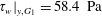
 $\unicode[STIX]{x1D70F}_{w}|_{y,G_{1}}=58.4~\text{Pa}$
over
$\unicode[STIX]{x1D70F}_{w}|_{y,G_{1}}=58.4~\text{Pa}$
over
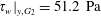 $\unicode[STIX]{x1D70F}_{w}|_{y,G_{2}}=51.2~\text{Pa}$
to
$\unicode[STIX]{x1D70F}_{w}|_{y,G_{2}}=51.2~\text{Pa}$
to
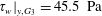 $\unicode[STIX]{x1D70F}_{w}|_{y,G_{3}}=45.5~\text{Pa}$
. Similarly the wall shear stress at the large side wall
$\unicode[STIX]{x1D70F}_{w}|_{y,G_{3}}=45.5~\text{Pa}$
. Similarly the wall shear stress at the large side wall
 $\unicode[STIX]{x1D70F}_{w}|_{z}$
reduces with increasing tangential grid resolution, see table 2. The point of maximum streamwise Reynolds stress
$\unicode[STIX]{x1D70F}_{w}|_{z}$
reduces with increasing tangential grid resolution, see table 2. The point of maximum streamwise Reynolds stress
 $\overline{u^{\prime }u^{\prime }}/u_{b}^{2}$
is moving closer to the wall and turbulence intensity increases slightly with falling
$\overline{u^{\prime }u^{\prime }}/u_{b}^{2}$
is moving closer to the wall and turbulence intensity increases slightly with falling
 $\unicode[STIX]{x0394}z_{max}/\unicode[STIX]{x0394}z_{min}$
. The same observation is made for
$\unicode[STIX]{x0394}z_{max}/\unicode[STIX]{x0394}z_{min}$
. The same observation is made for
 $\overline{v^{\prime }v^{\prime }}/u_{b}^{2}$
and
$\overline{v^{\prime }v^{\prime }}/u_{b}^{2}$
and
 $\overline{w^{\prime }w^{\prime }}/u_{b}^{2}$
. For all three grids
$\overline{w^{\prime }w^{\prime }}/u_{b}^{2}$
. For all three grids
 $9$
cells reside within the streamwise Reynolds stress maximum, respectively
$9$
cells reside within the streamwise Reynolds stress maximum, respectively
 $8$
cells at the large side walls. The comparison of
$8$
cells at the large side walls. The comparison of
 $G_{1}$
,
$G_{1}$
,
 $G_{2}$
and
$G_{2}$
and
 $G_{3}$
suggests for
$G_{3}$
suggests for
 $\unicode[STIX]{x0394}y_{max}/\unicode[STIX]{x0394}y_{min}$
, respectively
$\unicode[STIX]{x0394}y_{max}/\unicode[STIX]{x0394}y_{min}$
, respectively
 $\unicode[STIX]{x0394}z_{max}/\unicode[STIX]{x0394}z_{min}$
a value of
$\unicode[STIX]{x0394}z_{max}/\unicode[STIX]{x0394}z_{min}$
a value of
 ${\approx}25$
.
${\approx}25$
.

Figure 4. Grid sensitivity study with respect to (a,c,e) boundary layer velocity profile and (b,d,f) Reynolds stress distribution in the vicinity of the lower wall along the duct centre plane
 $z=0$
. The quantities are time- and streamwise-averaged for the adiabatic domain
$z=0$
. The quantities are time- and streamwise-averaged for the adiabatic domain
 $D_{per}$
. (a,b) Show the influence of the maximum wall-tangential cell size using
$D_{per}$
. (a,b) Show the influence of the maximum wall-tangential cell size using
 $G_{1}$
(——),
$G_{1}$
(——),
 $G_{2}$
(– - – - –) and
$G_{2}$
(– - – - –) and
 $G_{3}$
(- - - - - -), (c,d) the influence of the minimum cell size in the wall-normal direction using
$G_{3}$
(- - - - - -), (c,d) the influence of the minimum cell size in the wall-normal direction using
 $G_{1}$
(——),
$G_{1}$
(——),
 $G_{4}$
(– - – - –, blue) and
$G_{4}$
(– - – - –, blue) and
 $G_{5}$
(
$G_{5}$
(
 $\cdots \cdots$
, blue) and (e,f) the influence of the streamwise cell size using
$\cdots \cdots$
, blue) and (e,f) the influence of the streamwise cell size using
 $G_{1}$
(——),
$G_{1}$
(——),
 $G_{6}$
(– - – - –, orange) and
$G_{6}$
(– - – - –, orange) and
 $G_{7}$
(
$G_{7}$
(
 $\cdots \cdots$
, orange). See table 2 for reference. The classical law of the wall (
$\cdots \cdots$
, orange). See table 2 for reference. The classical law of the wall (
 $u^{+}=(1/0.41)\ln y^{+}+5.2$
) is represented by (
$u^{+}=(1/0.41)\ln y^{+}+5.2$
) is represented by (
 $\cdots \cdots$
, grey).
$\cdots \cdots$
, grey).
In figure 4(c,d) the minimum cell size in the wall-normal direction is modified, whereas the ratios of largest to smallest cell size
 $\unicode[STIX]{x0394}y_{max}/\unicode[STIX]{x0394}y_{min}$
and
$\unicode[STIX]{x0394}y_{max}/\unicode[STIX]{x0394}y_{min}$
and
 $\unicode[STIX]{x0394}z_{max}/\unicode[STIX]{x0394}z_{min}$
as well as the stretching factors
$\unicode[STIX]{x0394}z_{max}/\unicode[STIX]{x0394}z_{min}$
as well as the stretching factors
 $\unicode[STIX]{x1D6FE}_{y}$
and
$\unicode[STIX]{x1D6FE}_{y}$
and
 $\unicode[STIX]{x1D6FE}_{z}$
are approximately kept constant. As before, the cross-sectional discretisation is modified. The dimensionless wall distance
$\unicode[STIX]{x1D6FE}_{z}$
are approximately kept constant. As before, the cross-sectional discretisation is modified. The dimensionless wall distance
 $\unicode[STIX]{x0394}y_{min}^{+}$
varies from
$\unicode[STIX]{x0394}y_{min}^{+}$
varies from
 $\unicode[STIX]{x0394}y_{min}^{+}|_{G_{4}}=1.01$
over
$\unicode[STIX]{x0394}y_{min}^{+}|_{G_{4}}=1.01$
over
 $\unicode[STIX]{x0394}y_{min}^{+}|_{G_{1}}=1.28$
to
$\unicode[STIX]{x0394}y_{min}^{+}|_{G_{1}}=1.28$
to
 $\unicode[STIX]{x0394}y_{min}^{+}|_{G_{5}}=2.16$
. At the large side walls
$\unicode[STIX]{x0394}y_{min}^{+}|_{G_{5}}=2.16$
. At the large side walls
 $\unicode[STIX]{x0394}z_{min}^{+}$
is altered accordingly, see table 2. The comparison of
$\unicode[STIX]{x0394}z_{min}^{+}$
is altered accordingly, see table 2. The comparison of
 $G_{1}$
and
$G_{1}$
and
 $G_{4}$
verifies, that the resolution for
$G_{4}$
verifies, that the resolution for
 $G_{1}$
is sufficient to perform wall-resolved LES as the results coincide. A further coarsening of the wall-normal cell size leads to an underprediction of turbulent fluctuations without significant influence on the velocity profile. The wall resolution of
$G_{1}$
is sufficient to perform wall-resolved LES as the results coincide. A further coarsening of the wall-normal cell size leads to an underprediction of turbulent fluctuations without significant influence on the velocity profile. The wall resolution of
 $G_{5}$
is too coarse to resolve the Reynolds stress maximum correctly. Only
$G_{5}$
is too coarse to resolve the Reynolds stress maximum correctly. Only
 $6$
cells reside within the Reynolds stress maximum, for
$6$
cells reside within the Reynolds stress maximum, for
 $G_{4}$
this number is
$G_{4}$
this number is
 $10$
and for
$10$
and for
 $G_{1}$
9.
$G_{1}$
9.
Figure 4(e,f) depicts the influence of the streamwise cell size with
 $\unicode[STIX]{x0394}x^{+}|_{G_{1}}=98.6$
,
$\unicode[STIX]{x0394}x^{+}|_{G_{1}}=98.6$
,
 $\unicode[STIX]{x0394}x^{+}|_{G_{6}}=63.2$
and
$\unicode[STIX]{x0394}x^{+}|_{G_{6}}=63.2$
and
 $\unicode[STIX]{x0394}x^{+}|_{G_{7}}=47.1$
with an identical discretisation in the
$\unicode[STIX]{x0394}x^{+}|_{G_{7}}=47.1$
with an identical discretisation in the
 $yz$
-plane. We observe slight differences in the logarithmic region of the velocity profile, which get larger in the outer region. The finer discretisation in the streamwise direction leads to a reduction of the wall shear stress, which drops from
$yz$
-plane. We observe slight differences in the logarithmic region of the velocity profile, which get larger in the outer region. The finer discretisation in the streamwise direction leads to a reduction of the wall shear stress, which drops from
 $\unicode[STIX]{x1D70F}_{w}|_{y,G_{1}}=58.4~\text{Pa}$
to
$\unicode[STIX]{x1D70F}_{w}|_{y,G_{1}}=58.4~\text{Pa}$
to
 $\unicode[STIX]{x1D70F}_{w}|_{y,G_{6}}=55.8~\text{Pa}$
and
$\unicode[STIX]{x1D70F}_{w}|_{y,G_{6}}=55.8~\text{Pa}$
and
 $\unicode[STIX]{x1D70F}_{w}|_{y,G_{7}}=53.4~\text{Pa}$
,
$\unicode[STIX]{x1D70F}_{w}|_{y,G_{7}}=53.4~\text{Pa}$
,
 $u^{+}$
hence increases. Likewise, the Reynolds stresses are reduced uniformly. The maximum streamwise turbulence intensity
$u^{+}$
hence increases. Likewise, the Reynolds stresses are reduced uniformly. The maximum streamwise turbulence intensity
 $\overline{u^{\prime }u^{\prime }}$
expects a significant drop,
$\overline{u^{\prime }u^{\prime }}$
expects a significant drop,
 $\overline{v^{\prime }v^{\prime }}$
and
$\overline{v^{\prime }v^{\prime }}$
and
 $\overline{w^{\prime }w^{\prime }}$
just drop slightly over the whole interval. The maximum streamwise Reynolds stress
$\overline{w^{\prime }w^{\prime }}$
just drop slightly over the whole interval. The maximum streamwise Reynolds stress
 $\overline{u^{\prime }u^{\prime }}/u_{b}^{2}$
increases based on
$\overline{u^{\prime }u^{\prime }}/u_{b}^{2}$
increases based on
 $1.64\times 10^{-2}$
for the finest grid
$1.64\times 10^{-2}$
for the finest grid
 $G_{7}$
by 5.0 % for
$G_{7}$
by 5.0 % for
 $G_{6}$
and
$G_{6}$
and
 $13.8\,\%$
for
$13.8\,\%$
for
 $G_{1}$
. The location of the maximum turbulence intensity is not affected and is therefore only controlled by the cross-sectional grid resolution. Even though the streamwise turbulence intensity is slightly overpredicted,
$G_{1}$
. The location of the maximum turbulence intensity is not affected and is therefore only controlled by the cross-sectional grid resolution. Even though the streamwise turbulence intensity is slightly overpredicted,
 $\unicode[STIX]{x0394}x/\unicode[STIX]{x0394}y_{min}=50$
offers overall a good compromise between accuracy and numerical costs of the simulation.
$\unicode[STIX]{x0394}x/\unicode[STIX]{x0394}y_{min}=50$
offers overall a good compromise between accuracy and numerical costs of the simulation.
Based on the grid sensitivity analysis for the adiabatic duct the grid for the heated duct set-up is generated.
 $G_{6}$
serves as source grid, as the study has shown that it satisfies the aforementioned requirements for a well-resolved LES of the adiabatic duct at affordable numerical costs. The numerical parameters for the final grid are shown in table 3. For comparison with the sensitivity study, parameters for the adiabatic section
$G_{6}$
serves as source grid, as the study has shown that it satisfies the aforementioned requirements for a well-resolved LES of the adiabatic duct at affordable numerical costs. The numerical parameters for the final grid are shown in table 3. For comparison with the sensitivity study, parameters for the adiabatic section
 $D_{per}$
as well as the heated section
$D_{per}$
as well as the heated section
 $D_{heat}$
are listed. Both parameters at the refined heated wall at
$D_{heat}$
are listed. Both parameters at the refined heated wall at
 $y=y_{min}$
and the adiabatic wall at
$y=y_{min}$
and the adiabatic wall at
 $y=y_{max}$
are included. Note, that the evaluation of the wall shear stresses
$y=y_{max}$
are included. Note, that the evaluation of the wall shear stresses
 $\unicode[STIX]{x1D70F}_{w}$
and the inner length scale
$\unicode[STIX]{x1D70F}_{w}$
and the inner length scale
 $l^{+}$
for
$l^{+}$
for
 $D_{heat}$
is based on the streamwise-averaged flow condition over the last
$D_{heat}$
is based on the streamwise-averaged flow condition over the last
 $7.5\,d_{h}$
of the heated duct.
$7.5\,d_{h}$
of the heated duct.
For flows with
 $Pr>1$
, the thermal length scales are smaller than the momentum length scales and the temperature boundary layer is completely contained inside the momentum boundary layer. To resolve the wall-normal temperature gradient, the grid for the heated simulation is deduced from the adiabatic grid by increasing the resolution in the wall-normal direction at the heated wall, that is
$Pr>1$
, the thermal length scales are smaller than the momentum length scales and the temperature boundary layer is completely contained inside the momentum boundary layer. To resolve the wall-normal temperature gradient, the grid for the heated simulation is deduced from the adiabatic grid by increasing the resolution in the wall-normal direction at the heated wall, that is
 $y=y_{min}$
. The upper half of the duct as well as the blocking is left unaltered, see figure 3. The grid is only symmetric with respect to the
$y=y_{min}$
. The upper half of the duct as well as the blocking is left unaltered, see figure 3. The grid is only symmetric with respect to the
 $y$
-axis. The minimum cell size
$y$
-axis. The minimum cell size
 $\unicode[STIX]{x0394}y_{min}$
at the heated wall is reduced by the ratio of the smallest scales of the temperature field and the Kolmogorov scales following Monin, Yaglom & Lumley (Reference Monin, Yaglom and Lumley2007)
$\unicode[STIX]{x0394}y_{min}$
at the heated wall is reduced by the ratio of the smallest scales of the temperature field and the Kolmogorov scales following Monin, Yaglom & Lumley (Reference Monin, Yaglom and Lumley2007)
 $$\begin{eqnarray}\displaystyle \frac{\unicode[STIX]{x0394}y_{min}|_{heated}}{\unicode[STIX]{x0394}y_{min}|_{adiabatic}}=\frac{\unicode[STIX]{x1D702}_{\unicode[STIX]{x1D703}}}{\unicode[STIX]{x1D702}_{k}}=\left(\frac{1}{Pr}\right)^{1/2}, & & \displaystyle\end{eqnarray}$$
with
 $Pr=3.0$
, the value for water at
$Pr=3.0$
, the value for water at
 $T_{b}$
. As the Prandtl number drops with rising temperature, the resolution in the wall-normal direction is slightly finer than required. In contrast to the sensitivity analysis, we also apply for block
$T_{b}$
. As the Prandtl number drops with rising temperature, the resolution in the wall-normal direction is slightly finer than required. In contrast to the sensitivity analysis, we also apply for block
 $B_{2}$
a slight stretching in the
$B_{2}$
a slight stretching in the
 $y$
-direction.
$y$
-direction.

Figure 5. Comparison of (a) boundary layer velocity profile and (b) Reynolds stress distribution for the source grid
 $G_{6}$
(– - – - –, orange) and the final grid for the heated simulation at the
$G_{6}$
(– - – - –, orange) and the final grid for the heated simulation at the
 $y=y_{min}$
wall (——) and the
$y=y_{min}$
wall (——) and the
 $y=y_{max}$
wall (
$y=y_{max}$
wall (
 $\cdots \cdots$
) along the duct centre plane
$\cdots \cdots$
) along the duct centre plane
 $z=0$
. The quantities are time- and streamwise-averaged and evaluated for the adiabatic domain
$z=0$
. The quantities are time- and streamwise-averaged and evaluated for the adiabatic domain
 $D_{per}$
. See also tables 2 and 3 for reference. The classical law of the wall (
$D_{per}$
. See also tables 2 and 3 for reference. The classical law of the wall (
 $u^{+}=(1/0.41)\ln y^{+}+5.2$
) is represented by (
$u^{+}=(1/0.41)\ln y^{+}+5.2$
) is represented by (
 $\cdots \cdots$
, grey).
$\cdots \cdots$
, grey).
Figure 5 shows the comparison of mean velocity and Reynolds stress profiles for the source grid
 $G_{6}$
and the finally used grid for the heated simulation. For the latter both walls are shown, as a finer resolution is applied at the
$G_{6}$
and the finally used grid for the heated simulation. For the latter both walls are shown, as a finer resolution is applied at the
 $y=y_{min}$
wall, but both walls are modelled as adiabatic. The three velocity profiles coincide over a wide range, only in the outer layer a slight deviation is visible. The Reynolds stresses
$y=y_{min}$
wall, but both walls are modelled as adiabatic. The three velocity profiles coincide over a wide range, only in the outer layer a slight deviation is visible. The Reynolds stresses
 $\overline{w^{\prime }w^{\prime }}$
match, and only slight deviations in
$\overline{w^{\prime }w^{\prime }}$
match, and only slight deviations in
 $\overline{u^{\prime }u^{\prime }}$
and
$\overline{u^{\prime }u^{\prime }}$
and
 $\overline{v^{\prime }v^{\prime }}$
are present. At the large side walls eight cells reside within the streamwise Reynolds stress maximum, at the upper short side wall nine and at the lower short side wall
$\overline{v^{\prime }v^{\prime }}$
are present. At the large side walls eight cells reside within the streamwise Reynolds stress maximum, at the upper short side wall nine and at the lower short side wall
 $13$
for the adiabatic section and
$13$
for the adiabatic section and
 $11$
for the heated duct. As listed in table 3,
$11$
for the heated duct. As listed in table 3,
 $\unicode[STIX]{x0394}y_{min}^{+}$
drops to
$\unicode[STIX]{x0394}y_{min}^{+}$
drops to
 $0.73$
at the lower short side wall for the unheated section and to
$0.73$
at the lower short side wall for the unheated section and to
 $1.09$
when heating is applied. For the large side walls,
$1.09$
when heating is applied. For the large side walls,
 $\unicode[STIX]{x0394}z_{min}^{+}=1.42$
remains unchanged compared to the original grid
$\unicode[STIX]{x0394}z_{min}^{+}=1.42$
remains unchanged compared to the original grid
 $G_{6}$
. Note, that
$G_{6}$
. Note, that
 $\unicode[STIX]{x0394}y_{min}^{+}$
and
$\unicode[STIX]{x0394}y_{min}^{+}$
and
 $\unicode[STIX]{x0394}z_{min}^{+}$
are calculated with respect to the whole cell height of the respective first cell, whereas the flow variables are located and evaluated at the cell centre corresponding to
$\unicode[STIX]{x0394}z_{min}^{+}$
are calculated with respect to the whole cell height of the respective first cell, whereas the flow variables are located and evaluated at the cell centre corresponding to
 $z_{min}^{+}=0.71$
and
$z_{min}^{+}=0.71$
and
 $y_{min}^{+}=0.37$
, respectively
$y_{min}^{+}=0.37$
, respectively
 $y_{min}^{+}=0.55$
, in a finite difference sense. A comparison of the adiabatic duct wall shear stresses
$y_{min}^{+}=0.55$
, in a finite difference sense. A comparison of the adiabatic duct wall shear stresses
 $\unicode[STIX]{x1D70F}_{w}|_{y}$
for the upper and lower short wall shows, that the unequal meshes have a negligible effect.
$\unicode[STIX]{x1D70F}_{w}|_{y}$
for the upper and lower short wall shows, that the unequal meshes have a negligible effect.
4 Comparison with experimental data
The numerical results for the heated duct are compared with the experimental data both qualitatively using the PTV results and quantitatively using the PIV results in the duct centre (Rochlitz et al.
Reference Rochlitz, Scholz and Fuchs2015). The flow quantities of the LES are temporally averaged over
 $20$
FTT and subsequently, identical to the experimental data, spatially averaged over the FOV, see figure 1.
$20$
FTT and subsequently, identical to the experimental data, spatially averaged over the FOV, see figure 1.

Figure 6. Comparison of streamwise velocity distribution in the cross-section of the heated duct averaged over the FOV, see figure 1 for reference. The heated wall is located at
 $y=y_{min}$
. Due to reflections, experimental data in the vicinity of the walls are cut-off.
$y=y_{min}$
. Due to reflections, experimental data in the vicinity of the walls are cut-off.
Figure 6 illustrates the good qualitative agreement of the experimental PTV results and the LES for the heated duct. We observe two minor deviations. First, the streamwise velocity
 $\overline{u}/u_{b}$
in the duct core is slightly larger in the LES, the maximum value
$\overline{u}/u_{b}$
in the duct core is slightly larger in the LES, the maximum value
 $(\overline{u}/u_{b})_{max}$
is
$(\overline{u}/u_{b})_{max}$
is
 $1.83\,\%$
higher. We attribute this deviation to the wider duct of the experiment due to the fabrication tolerances decreasing the core velocity. Second, the LES flow field possesses a higher symmetry. Following Rochlitz et al. (Reference Rochlitz, Scholz and Fuchs2015) the asymmetry of the experimental data is probably caused by a slight laser sheet misalignment as it is also observed for the unheated flow. The slight asymmetry in the LES is attributed to the asymmetrically applied heat flux.
$1.83\,\%$
higher. We attribute this deviation to the wider duct of the experiment due to the fabrication tolerances decreasing the core velocity. Second, the LES flow field possesses a higher symmetry. Following Rochlitz et al. (Reference Rochlitz, Scholz and Fuchs2015) the asymmetry of the experimental data is probably caused by a slight laser sheet misalignment as it is also observed for the unheated flow. The slight asymmetry in the LES is attributed to the asymmetrically applied heat flux.

Figure 7. Comparison of experimental (
 $\cdots \cdots$
) and numerical results for the heated duct centre plane averaged in the streamwise direction over the FOV. The unmodified LES results are marked by (——) and the results modified by laser sheet averaging with
$\cdots \cdots$
) and numerical results for the heated duct centre plane averaged in the streamwise direction over the FOV. The unmodified LES results are marked by (——) and the results modified by laser sheet averaging with
 $\unicode[STIX]{x0394}LS=1~\text{mm}$
and aspect ratio compensation by (– - – - –, blue). (a,b) Show the streamwise and heated wall-normal velocity and (c–e) the Reynolds stress distribution. Experimental and numerical results are made dimensionless using the respective
$\unicode[STIX]{x0394}LS=1~\text{mm}$
and aspect ratio compensation by (– - – - –, blue). (a,b) Show the streamwise and heated wall-normal velocity and (c–e) the Reynolds stress distribution. Experimental and numerical results are made dimensionless using the respective
 $u_{b}$
and
$u_{b}$
and
 $L_{y}$
.
$L_{y}$
.
In the following, we compare the LES results with the PIV results in the duct centre plane, i.e. the velocity profiles along the heated wall-normal direction. In order to approximate the filter effect of the PIV technique, we postprocess the LES velocity profiles based on the cross-sectional flow field by a weighted averaging across the duct centre plane, in this case the
 $y$
-axis, corresponding to a finite laser sheet thickness
$y$
-axis, corresponding to a finite laser sheet thickness
 $\unicode[STIX]{x0394}LS\approx 1~\text{mm}$
. The weighting is performed by assuming a Gaussian laser intensity distribution.
$\unicode[STIX]{x0394}LS\approx 1~\text{mm}$
. The weighting is performed by assuming a Gaussian laser intensity distribution.
Due to the manufacturing tolerances, the experimental and numerical duct geometries are slightly different, resulting in an experimental aspect ratio of
 $AR_{exp}=4.19$
and
$AR_{exp}=4.19$
and
 $AR_{LES}=4.30$
for the simulations. The ducts aspect ratio defines the location of the corner vortices, which in turn has an impact on the streamwise and wall-normal velocity profiles in the duct centre. Especially the positions of the
$AR_{LES}=4.30$
for the simulations. The ducts aspect ratio defines the location of the corner vortices, which in turn has an impact on the streamwise and wall-normal velocity profiles in the duct centre. Especially the positions of the
 $\overline{v}$
-velocity peaks and the resulting shoulders in the
$\overline{v}$
-velocity peaks and the resulting shoulders in the
 $\overline{u}$
-profile are hereby defined. To account for the slight aspect ratio deviation and the accompanying shift of the vortex positions, we introduce an
$\overline{u}$
-profile are hereby defined. To account for the slight aspect ratio deviation and the accompanying shift of the vortex positions, we introduce an
 $AR$
-compensation to the LES data by rescaling
$AR$
-compensation to the LES data by rescaling
 $y=y_{LES}\,(AR_{exp}/AR_{LES})$
. Comparing the unmodified LES results with the ones modified by laser sheet averaging and aspect ratio compensation in figure 7, one can see that the postprocessing leads to a better agreement with the experimental data in the near-wall regions of the
$y=y_{LES}\,(AR_{exp}/AR_{LES})$
. Comparing the unmodified LES results with the ones modified by laser sheet averaging and aspect ratio compensation in figure 7, one can see that the postprocessing leads to a better agreement with the experimental data in the near-wall regions of the
 $\overline{u}$
-profile until the shoulder section. Likewise, the peak positions of the
$\overline{u}$
-profile until the shoulder section. Likewise, the peak positions of the
 $\overline{v}$
-profile are shifted away from the lower and upper wall. The velocity magnitudes drop slightly due to the laser sheet averaging.
$\overline{v}$
-profile are shifted away from the lower and upper wall. The velocity magnitudes drop slightly due to the laser sheet averaging.
For the velocity profile in figure 7(a), very good agreement can be observed in the vicinity of the walls until approximately
 $2y/L_{y}=\pm 0.75$
. The shoulder section in the interval from
$2y/L_{y}=\pm 0.75$
. The shoulder section in the interval from
 $-0.75$
to
$-0.75$
to
 $-0.5$
is in good agreement with the experimental data. The shoulder section at the opposite wall exhibits larger deviations due to the slight asymmetry of the experimental data. As pointed out in the qualitative comparison, the streamwise velocity in the duct core is slightly higher because of the narrower cross-section. Compared to the PIV results,
$-0.5$
is in good agreement with the experimental data. The shoulder section at the opposite wall exhibits larger deviations due to the slight asymmetry of the experimental data. As pointed out in the qualitative comparison, the streamwise velocity in the duct core is slightly higher because of the narrower cross-section. Compared to the PIV results,
 $(\overline{u}/u_{b})_{max}$
is
$(\overline{u}/u_{b})_{max}$
is
 $1.71\,\%$
larger. The numerical and experimental
$1.71\,\%$
larger. The numerical and experimental
 $\overline{v}$
-profiles agree very well. The peak positions indicating the influence of the corner vortices on the duct centre match almost perfectly, the maximum values, however, are again slightly higher. The deviation for the
$\overline{v}$
-profiles agree very well. The peak positions indicating the influence of the corner vortices on the duct centre match almost perfectly, the maximum values, however, are again slightly higher. The deviation for the
 $\overline{v}$
-minimum at the
$\overline{v}$
-minimum at the
 $y=y_{max}$
wall is larger than for the other three extrema. We attribute this deviation to the aforementioned asymmetry of the experimental data.
$y=y_{max}$
wall is larger than for the other three extrema. We attribute this deviation to the aforementioned asymmetry of the experimental data.
The streamwise Reynolds stress
 $\overline{u^{\prime }u^{\prime }}$
shows a satisfactory agreement with the LES having consistently lower values than the PIV, see figure 7(c). This difference is probably due to measurement noise. The
$\overline{u^{\prime }u^{\prime }}$
shows a satisfactory agreement with the LES having consistently lower values than the PIV, see figure 7(c). This difference is probably due to measurement noise. The
 $\overline{u^{\prime }v^{\prime }}$
profiles match very well except in the vicinity of the walls, where the LES has higher extrema. The wall-normal Reynolds stresses
$\overline{u^{\prime }v^{\prime }}$
profiles match very well except in the vicinity of the walls, where the LES has higher extrema. The wall-normal Reynolds stresses
 $\overline{v^{\prime }v^{\prime }}$
coincide in the vicinity of the heated wall. In the duct centre, we observe a similar offset like that in
$\overline{v^{\prime }v^{\prime }}$
coincide in the vicinity of the heated wall. In the duct centre, we observe a similar offset like that in
 $\overline{u^{\prime }u^{\prime }}$
. At the upper wall large deviations are visible due to an overshoot in the experimental data. We assume, that the random component of the measurement error is essentially uncorrelated Gaussian noise. Thus it increases the autocorrelations
$\overline{u^{\prime }u^{\prime }}$
. At the upper wall large deviations are visible due to an overshoot in the experimental data. We assume, that the random component of the measurement error is essentially uncorrelated Gaussian noise. Thus it increases the autocorrelations
 $\overline{u^{\prime }u^{\prime }}$
and
$\overline{u^{\prime }u^{\prime }}$
and
 $\overline{v^{\prime }v^{\prime }}$
, but has no effect on the cross-correlation
$\overline{v^{\prime }v^{\prime }}$
, but has no effect on the cross-correlation
 $\overline{u^{\prime }v^{\prime }}$
in the core flow. Near the walls, PIV suffers from spurious reflections and low seeding density.
$\overline{u^{\prime }v^{\prime }}$
in the core flow. Near the walls, PIV suffers from spurious reflections and low seeding density.
Following Rochlitz et al. (Reference Rochlitz, Scholz and Fuchs2015), the measurements exhibit uncertainties with respect to the laser sheet misalignment and the effective laser sheet thickness. The latter may be larger than the reported value of
 $\unicode[STIX]{x0394}LS=1~\text{mm}$
. We have investigated the influence of these uncertainties on the numerical data and observed that the agreement of numerical and experimental data, for both velocity and Reynolds stresses, is improved by taking a slight misalignment and an effective laser sheet thickness larger than
$\unicode[STIX]{x0394}LS=1~\text{mm}$
. We have investigated the influence of these uncertainties on the numerical data and observed that the agreement of numerical and experimental data, for both velocity and Reynolds stresses, is improved by taking a slight misalignment and an effective laser sheet thickness larger than
 $1~\text{mm}$
into account.
$1~\text{mm}$
into account.
For the accuracy assessment of our well-resolved LES, we refer to the comparison of an adiabatic square duct LES at a comparable grid resolution as the cooling duct simulation with DNS results in Appendix A.
5 Results and discussion
5.1 Mean flow field of the adiabatic and heated duct
In the following we analyse the turbulent heat transfer in the asymmetrically heated duct based on the LES results. The main focus lies on investigating the differences of the adiabatic and the heated duct flow field, i.e. on the influence of the wall heating along the duct. Due to the heating, the temperature in the vicinity of the lower wall increases with streamwise distance, reducing the local viscosity, which may drop up to
 $\unicode[STIX]{x1D708}(T_{w})=0.62\,\unicode[STIX]{x1D708}(T_{b})$
.
$\unicode[STIX]{x1D708}(T_{w})=0.62\,\unicode[STIX]{x1D708}(T_{b})$
.

Figure 8. Streamwise flow field in the duct cross-section of the adiabatic duct with (a) instantaneous streamwise velocity, (b) mean streamwise velocity and (c) mean streamwise velocity with additional averaging of the four quadrants. The contour lines are drawn in steps of
 $0.1$
.
$0.1$
.
Figure 8 displays the cross-section streamwise flow field for the adiabatic duct: an instantaneous snapshot in (a) and the mean solution in (b,c). The instantaneous velocity field shows the highly turbulent flow with the highest velocities in the duct core and smaller low-velocity structures along the side walls and in the duct corners. For the mean solution a temporal averaging over
 $164$
FTT with respect to the periodic section at a constant sampling rate of
$164$
FTT with respect to the periodic section at a constant sampling rate of
 $\unicode[STIX]{x0394}t_{sample}=0.025\,d_{h}/u_{b}$
is performed, resulting in
$\unicode[STIX]{x0394}t_{sample}=0.025\,d_{h}/u_{b}$
is performed, resulting in
 ${\approx}50\times 10^{3}$
snapshots. Additionally, a spatial averaging in the streamwise direction is applied. For the quadrant-averaged solution a further averaging over the four quadrants is done exploiting the duct symmetry in order to reduce the number of samples required for a statistically convergent result. As Vinuesa et al. (Reference Vinuesa, Noorani, Lozano-Duran, El Khoury, Schlatter, Fischer and Nagib2014) pointed out, the number of required samples is not reduced by a factor of four as the flow in the quadrants is not independent, in particular the corner vortices in the vicinity of the short side walls are strongly correlated. As a convergence measure we utilise the symmetry of the flow field. The comparison of figure 8(b,c) shows that the streamwise velocity field is sufficiently converged as hardly any difference is visible. The L2 norm of the streamwise velocity deviation between the not-quadrant-averaged and the quadrant-averaged result in the
${\approx}50\times 10^{3}$
snapshots. Additionally, a spatial averaging in the streamwise direction is applied. For the quadrant-averaged solution a further averaging over the four quadrants is done exploiting the duct symmetry in order to reduce the number of samples required for a statistically convergent result. As Vinuesa et al. (Reference Vinuesa, Noorani, Lozano-Duran, El Khoury, Schlatter, Fischer and Nagib2014) pointed out, the number of required samples is not reduced by a factor of four as the flow in the quadrants is not independent, in particular the corner vortices in the vicinity of the short side walls are strongly correlated. As a convergence measure we utilise the symmetry of the flow field. The comparison of figure 8(b,c) shows that the streamwise velocity field is sufficiently converged as hardly any difference is visible. The L2 norm of the streamwise velocity deviation between the not-quadrant-averaged and the quadrant-averaged result in the
 $yz$
-plane is
$yz$
-plane is
 $0.5\,\%$
.
$0.5\,\%$
.

Figure 9. Secondary flow field in the duct cross-section of the adiabatic duct with (a) mean cross-flow velocity magnitude
 $\overline{u}_{cf}=\sqrt{\overline{v}^{2}+\overline{w}^{2}}$
, (b) mean cross-flow velocity magnitude
$\overline{u}_{cf}=\sqrt{\overline{v}^{2}+\overline{w}^{2}}$
, (b) mean cross-flow velocity magnitude
 $\overline{u}_{cf}$
with an additional averaging of the four quadrants and (c) counter-rotating corner vortices represented by streamlines. The contour lines are drawn in steps of
$\overline{u}_{cf}$
with an additional averaging of the four quadrants and (c) counter-rotating corner vortices represented by streamlines. The contour lines are drawn in steps of
 $0.15\times 10^{-2}$
.
$0.15\times 10^{-2}$
.
In general, the convergence rate of the turbulence-induced secondary flow is slower than that of the streamwise velocity. Figure 9 depicts the secondary flow field represented by the cross-flow velocity magnitude
 $\overline{u}_{cf}=\sqrt{\overline{v}^{2}+\overline{w}^{2}}$
and streamlines. The comparison with the quadrant-averaged solution in figure 9(b) shows that the result is not perfectly converged as the secondary flow field is slightly asymmetric. The deviation from the symmetric state is higher than for the streamwise velocity, but sufficiently small. A reason for the larger deviation is the presence of very weak vortices in the duct centre, see figure 9(c). These persist over very long averaging times. Such a formation of an array of secondary vortices along the long side walls of high aspect ducts has been observed previously by Vinuesa et al. (Reference Vinuesa, Noorani, Lozano-Duran, El Khoury, Schlatter, Fischer and Nagib2014).
$\overline{u}_{cf}=\sqrt{\overline{v}^{2}+\overline{w}^{2}}$
and streamlines. The comparison with the quadrant-averaged solution in figure 9(b) shows that the result is not perfectly converged as the secondary flow field is slightly asymmetric. The deviation from the symmetric state is higher than for the streamwise velocity, but sufficiently small. A reason for the larger deviation is the presence of very weak vortices in the duct centre, see figure 9(c). These persist over very long averaging times. Such a formation of an array of secondary vortices along the long side walls of high aspect ducts has been observed previously by Vinuesa et al. (Reference Vinuesa, Noorani, Lozano-Duran, El Khoury, Schlatter, Fischer and Nagib2014).

Figure 10. Cross-sectional temperature distribution and its streamwise development in (a–f) and development of the secondary flow velocity in the vicinity of the heated wall, exemplarily shown for the heated wall-normal component in (g–l). (a,g) Depicts the adiabatic duct, (b,h) the heated duct after
 $50~\text{mm}$
, (c,i) after
$50~\text{mm}$
, (c,i) after
 $100~\text{mm}$
, (d,j) after
$100~\text{mm}$
, (d,j) after
 $200~\text{mm}$
, (e,k) after
$200~\text{mm}$
, (e,k) after
 $400~\text{mm}$
and (f,l) after
$400~\text{mm}$
and (f,l) after
 $600~\text{mm}$
. In (a–f), the cross-flow velocity vectors indicate the influence of the secondary flow motions on the temperature distribution and the contour lines are drawn in steps of
$600~\text{mm}$
. In (a–f), the cross-flow velocity vectors indicate the influence of the secondary flow motions on the temperature distribution and the contour lines are drawn in steps of
 $2~\text{K}$
. In (g–l), the wall-normal velocity
$2~\text{K}$
. In (g–l), the wall-normal velocity
 $\overline{v}$
is depicted on the left of the duct centre and on the right the change in
$\overline{v}$
is depicted on the left of the duct centre and on the right the change in
 $\overline{v}$
with respect to the unheated periodic duct,
$\overline{v}$
with respect to the unheated periodic duct,
 $\unicode[STIX]{x0394}\overline{v}=\overline{v}-\overline{v}_{per}$
, is shown. The contour lines are drawn in steps of
$\unicode[STIX]{x0394}\overline{v}=\overline{v}-\overline{v}_{per}$
, is shown. The contour lines are drawn in steps of
 $\overline{v}/u_{b}=0.002$
.
$\overline{v}/u_{b}=0.002$
.
The developing temperature boundary layer along the heated duct length is highly affected by the secondary flow structures. Figure 9(c) shows the pairs of counter-rotating vortices forming in each of the duct corners. In the left upper corner (
 $y<0$
,
$y<0$
,
 $z>0$
), a small counter-clockwise (CCW) rotating vortex forms along the short side wall and a large clockwise (CW) rotating vortex along the long side wall (mirror inverted for the opposite half of the duct). Each vortex extends to the respective symmetry plane, where it encounters the neighbouring vortex from the opposite side. The vortex strength is relatively weak. The maximum cross-flow velocity for the adiabatic duct is
$z>0$
), a small counter-clockwise (CCW) rotating vortex forms along the short side wall and a large clockwise (CW) rotating vortex along the long side wall (mirror inverted for the opposite half of the duct). Each vortex extends to the respective symmetry plane, where it encounters the neighbouring vortex from the opposite side. The vortex strength is relatively weak. The maximum cross-flow velocity for the adiabatic duct is
 $\overline{u}_{cf}/u_{b}=1.93\,\%$
, which lies within the 1–3 % range reported in the literature, see for example Salinas-Vásquez & Métais (Reference Salinas-Vásquez and Métais2002). Figure 10(a–f) depict the axial development of the temperature boundary layer at different positions along the heated duct section for the lower duct quarter. The thermal boundary layer thickness increases in the streamwise direction due to conduction, turbulent mixing and through transport by the mean secondary flow. The latter is responsible for the characteristic bent shape of the temperature profile. In the left half of the duct, the CW vortex transports hot fluid away from the heated wall along the long side wall into the duct core and cold fluid downwards along the centre line. The CCW vortex conveys hot fluid from the corner along the heated wall to its centre at
$\overline{u}_{cf}/u_{b}=1.93\,\%$
, which lies within the 1–3 % range reported in the literature, see for example Salinas-Vásquez & Métais (Reference Salinas-Vásquez and Métais2002). Figure 10(a–f) depict the axial development of the temperature boundary layer at different positions along the heated duct section for the lower duct quarter. The thermal boundary layer thickness increases in the streamwise direction due to conduction, turbulent mixing and through transport by the mean secondary flow. The latter is responsible for the characteristic bent shape of the temperature profile. In the left half of the duct, the CW vortex transports hot fluid away from the heated wall along the long side wall into the duct core and cold fluid downwards along the centre line. The CCW vortex conveys hot fluid from the corner along the heated wall to its centre at
 $z=0$
and then upwards along the symmetry line until it mixes with the cold fluid transported downwards. Both vortices push cold fluid into the left corner, whereby the flow vectors follow a slightly flatter path than the corners bisecting line.
$z=0$
and then upwards along the symmetry line until it mixes with the cold fluid transported downwards. Both vortices push cold fluid into the left corner, whereby the flow vectors follow a slightly flatter path than the corners bisecting line.
Even though the temperature increase and the accompanying viscosity decrease are overall relatively moderate, we observe a significant weakening of the secondary flow strength in figure 10(g–l), where the heated wall-normal secondary flow component
 $\overline{v}$
is shown at the same spatial positions along the heated duct section as the temperature boundary layer in figure 10(a–f). In the left half of each picture the mean vertical velocity
$\overline{v}$
is shown at the same spatial positions along the heated duct section as the temperature boundary layer in figure 10(a–f). In the left half of each picture the mean vertical velocity
 $\overline{v}$
is depicted and in the right half the difference of the
$\overline{v}$
is depicted and in the right half the difference of the
 $\overline{v}$
-field with respect to the adiabatic case,
$\overline{v}$
-field with respect to the adiabatic case,
 $\unicode[STIX]{x0394}\overline{v}=\overline{v}-\overline{v}_{per}$
. We observe a significant reduction of the vortex strength. The upward transport of hot fluid in the vicinity of the lateral wall is slowed down increasingly, in the end cross-section the maximum
$\unicode[STIX]{x0394}\overline{v}=\overline{v}-\overline{v}_{per}$
. We observe a significant reduction of the vortex strength. The upward transport of hot fluid in the vicinity of the lateral wall is slowed down increasingly, in the end cross-section the maximum
 $\unicode[STIX]{x0394}\overline{v}/u_{b}$
is
$\unicode[STIX]{x0394}\overline{v}/u_{b}$
is
 ${\approx}-0.004$
with a velocity of
${\approx}-0.004$
with a velocity of
 $\overline{v}/u_{b}\approx 0.015$
, which corresponds to a reduction of more than
$\overline{v}/u_{b}\approx 0.015$
, which corresponds to a reduction of more than
 $25\,\%$
. The positions of the corner vortices change only a little, thus they are mainly defined by the duct geometry. The small CCW vortex centre moves from
$25\,\%$
. The positions of the corner vortices change only a little, thus they are mainly defined by the duct geometry. The small CCW vortex centre moves from
 $(2y/L_{y},2z/L_{z})=(-0.947,0.414)$
for the adiabatic duct to (
$(2y/L_{y},2z/L_{z})=(-0.947,0.414)$
for the adiabatic duct to (
 $-0.948$
,
$-0.948$
,
 $0.394$
) at position
$0.394$
) at position
 $600~\text{mm}$
and the large CW vortex centre from (
$600~\text{mm}$
and the large CW vortex centre from (
 $-0.752$
,
$-0.752$
,
 $0.569$
) to (
$0.569$
) to (
 $-0.763$
,
$-0.763$
,
 $0.601$
). Hence, we observe for the large vortex a slight shift towards both side walls and for the small one a slight shift towards the midplane.
$0.601$
). Hence, we observe for the large vortex a slight shift towards both side walls and for the small one a slight shift towards the midplane.
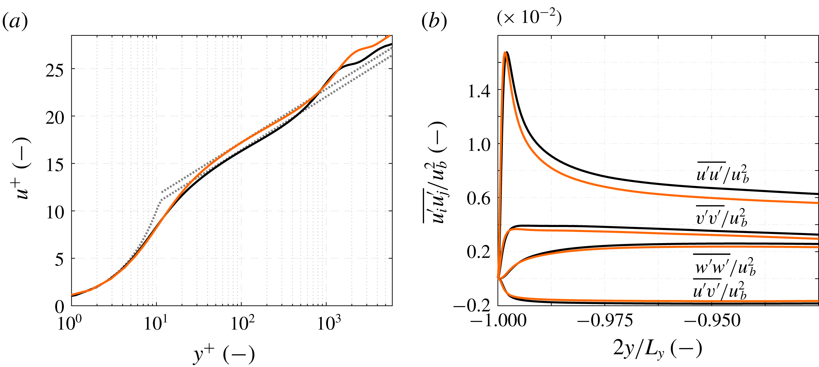
Figure 11. Profiles of (a) mean streamwise velocity and (b) Reynolds stresses along the duct midplane at
 $z=0$
for the adiabatic (——) and the heated duct (——, orange). The law of the wall is represented by (
$z=0$
for the adiabatic (——) and the heated duct (——, orange). The law of the wall is represented by (
 $\cdots \cdots$
, grey).
$\cdots \cdots$
, grey).
As the corner vortices are turbulence-induced secondary flow structures, we further analyse the influence of the reduced wall viscosity on the mean turbulence and velocity profiles. In figure 11, we investigate the influence of the wall heating on the turbulent boundary layer in the duct centre at
 $z=0$
by comparing the spatially averaged solutions over the adiabatic domain
$z=0$
by comparing the spatially averaged solutions over the adiabatic domain
 $D_{per}$
and the last
$D_{per}$
and the last
 $7.5\,d_{h}$
of the heated duct. For both sections good agreement with the classical law of the wall velocity profile is obtained,
$7.5\,d_{h}$
of the heated duct. For both sections good agreement with the classical law of the wall velocity profile is obtained,
 $u^{+}=y^{+}$
for the viscous sublayer and
$u^{+}=y^{+}$
for the viscous sublayer and
 $u^{+}=(1/\unicode[STIX]{x1D705})\ln y^{+}+B$
for the log-law region. Like Lee et al. (Reference Lee, Jung, Sung and Zaki2013), we observe in figure 11 (a) that the heating leads to an upwards shift in the log-law region of the velocity profile, the integration constant increases from
$u^{+}=(1/\unicode[STIX]{x1D705})\ln y^{+}+B$
for the log-law region. Like Lee et al. (Reference Lee, Jung, Sung and Zaki2013), we observe in figure 11 (a) that the heating leads to an upwards shift in the log-law region of the velocity profile, the integration constant increases from
 $B=5.2$
to
$B=5.2$
to
 $B=6.0$
for the heated case. The slope, i.e. the von Kármán constant remains unchanged at
$B=6.0$
for the heated case. The slope, i.e. the von Kármán constant remains unchanged at
 $\unicode[STIX]{x1D705}=0.41$
. Figure 11(b) depicts the change in the Reynolds stress profiles. The peak in
$\unicode[STIX]{x1D705}=0.41$
. Figure 11(b) depicts the change in the Reynolds stress profiles. The peak in
 $\overline{u^{\prime }u^{\prime }}$
shifts slightly closer to the wall, whereas the maximum value remains unaltered. Similarly to Zonta, Marchioli & Soldati (Reference Zonta, Marchioli and Soldati2012), we observe that the turbulence intensities in all directions are reduced, when heating is applied to the flow. Although counterintuitive, as one would expect an increase in turbulent fluctuations with lower viscosity, this observation is in agreement with previous studies showing that the heating of the fluid accompanied by a drop in viscosity has a stabilising effect on the boundary layer, see Lee et al. (Reference Lee, Jung, Sung and Zaki2013) and Zonta et al. (Reference Zonta, Marchioli and Soldati2012).
$\overline{u^{\prime }u^{\prime }}$
shifts slightly closer to the wall, whereas the maximum value remains unaltered. Similarly to Zonta, Marchioli & Soldati (Reference Zonta, Marchioli and Soldati2012), we observe that the turbulence intensities in all directions are reduced, when heating is applied to the flow. Although counterintuitive, as one would expect an increase in turbulent fluctuations with lower viscosity, this observation is in agreement with previous studies showing that the heating of the fluid accompanied by a drop in viscosity has a stabilising effect on the boundary layer, see Lee et al. (Reference Lee, Jung, Sung and Zaki2013) and Zonta et al. (Reference Zonta, Marchioli and Soldati2012).

Figure 12. Distribution of the mean velocity components and mean temperature difference along the heated wall-normal direction at the spanwise positions of (a)
 $2z/L_{z}=0$
, (b)
$2z/L_{z}=0$
, (b)
 $2z/L_{z}=0.5$
and (c)
$2z/L_{z}=0.5$
and (c)
 $2z/L_{z}=0.9$
for the adiabatic duct (——) and the heated duct at a streamwise position of
$2z/L_{z}=0.9$
for the adiabatic duct (——) and the heated duct at a streamwise position of
 $100~\text{mm}$
(
$100~\text{mm}$
(
 $\cdots \cdots$
, orange), respectively
$\cdots \cdots$
, orange), respectively
 $595~\text{mm}$
(– - – - –, orange) after the beginning of the heated section. Streamwise averaging has been performed over
$595~\text{mm}$
(– - – - –, orange) after the beginning of the heated section. Streamwise averaging has been performed over
 $10~\text{mm}$
for the heated duct, respectively over
$10~\text{mm}$
for the heated duct, respectively over
 $L_{x,per}$
for the periodic duct, and the
$L_{x,per}$
for the periodic duct, and the
 $y$
-symmetry is utilised.
$y$
-symmetry is utilised.

Figure 13. Distribution of the diagonal components of the Reynolds stress tensor along the heated wall-normal direction at the spanwise positions of (a)
 $2z/L_{z}=0$
, (b)
$2z/L_{z}=0$
, (b)
 $2z/L_{z}=0.5$
and (c)
$2z/L_{z}=0.5$
and (c)
 $2z/L_{z}=0.9$
for the adiabatic duct (——) and the heated duct at a streamwise position of
$2z/L_{z}=0.9$
for the adiabatic duct (——) and the heated duct at a streamwise position of
 $100~\text{mm}$
(
$100~\text{mm}$
(
 $\cdots \cdots$
, orange), respectively
$\cdots \cdots$
, orange), respectively
 $595~\text{mm}$
(– - – - –, orange) after the beginning of the heated section. Streamwise averaging has been performed over
$595~\text{mm}$
(– - – - –, orange) after the beginning of the heated section. Streamwise averaging has been performed over
 $10~\text{mm}$
for the heated duct, respectively over
$10~\text{mm}$
for the heated duct, respectively over
 $L_{x,per}$
for the periodic duct, and the
$L_{x,per}$
for the periodic duct, and the
 $y$
-symmetry is utilised.
$y$
-symmetry is utilised.

Figure 14. Distribution of the off-diagonal components of the Reynolds stress tensor along the heated wall-normal direction at the spanwise positions of (a)
 $2z/L_{z}=0$
, (b)
$2z/L_{z}=0$
, (b)
 $2z/L_{z}=0.5$
and (c)
$2z/L_{z}=0.5$
and (c)
 $2z/L_{z}=0.9$
for the adiabatic duct (——) and the heated duct at a streamwise position of
$2z/L_{z}=0.9$
for the adiabatic duct (——) and the heated duct at a streamwise position of
 $100~\text{mm}$
(
$100~\text{mm}$
(
 $\cdots \cdots$
, orange), respectively
$\cdots \cdots$
, orange), respectively
 $595~\text{mm}$
(– - – - –, orange) after the beginning of the heated section. Streamwise averaging has been performed over
$595~\text{mm}$
(– - – - –, orange) after the beginning of the heated section. Streamwise averaging has been performed over
 $10~\text{mm}$
for the heated duct, respectively over
$10~\text{mm}$
for the heated duct, respectively over
 $L_{x,per}$
for the periodic duct, and the
$L_{x,per}$
for the periodic duct, and the
 $y$
-symmetry is utilised.
$y$
-symmetry is utilised.
In figures 12–14 we present the mean velocity, temperature and Reynolds stress distributions for three different
 $z$
-locations, for the duct centre at
$z$
-locations, for the duct centre at
 $2z/L_{z}=0$
, at
$2z/L_{z}=0$
, at
 $2z/L_{z}=0.5$
and at
$2z/L_{z}=0.5$
and at
 $2z/L_{z}=0.9$
. All figures compare the results for the adiabatic duct with those for the heated duct at
$2z/L_{z}=0.9$
. All figures compare the results for the adiabatic duct with those for the heated duct at
 $100~\text{mm}$
and
$100~\text{mm}$
and
 $595~\text{mm}$
after beginning of the heated section. For the adiabatic duct streamwise averaging is performed over
$595~\text{mm}$
after beginning of the heated section. For the adiabatic duct streamwise averaging is performed over
 $L_{x,per}$
and for the heated duct over a
$L_{x,per}$
and for the heated duct over a
 $10~\text{mm}$
interval from
$10~\text{mm}$
interval from
 $-5~\text{mm}$
to
$-5~\text{mm}$
to
 $+5~\text{mm}$
of the respective location.
$+5~\text{mm}$
of the respective location.
Moving outwards from the duct centre towards the lateral wall, i.e. from figure 12(a–c), we observe for the adiabatic case a broadening of the
 $\overline{u}$
-profiles shoulder section, which is formed as a consequence of the corner vortex pair. The asymmetric heating applied to the duct leads to a mass flux redistribution. The flow in the lower quarter of the duct below
$\overline{u}$
-profiles shoulder section, which is formed as a consequence of the corner vortex pair. The asymmetric heating applied to the duct leads to a mass flux redistribution. The flow in the lower quarter of the duct below
 $2y/L_{y}\approx 0.5$
is accelerated leading to a thickening of the near-wall profile. This behaviour is qualitatively consistent with previous channel flow and TBL studies by Sameen & Govindarajan (Reference Sameen and Govindarajan2007) and Lee et al. (Reference Lee, Jung, Sung and Zaki2013). Moreover, the heated duct
$2y/L_{y}\approx 0.5$
is accelerated leading to a thickening of the near-wall profile. This behaviour is qualitatively consistent with previous channel flow and TBL studies by Sameen & Govindarajan (Reference Sameen and Govindarajan2007) and Lee et al. (Reference Lee, Jung, Sung and Zaki2013). Moreover, the heated duct
 $\overline{u}$
-profile exhibits a more pronounced shoulder section due to the weaker secondary flow and the accompanying reduced vertical momentum transport. In the duct core, the streamwise velocity drops slightly compared to the adiabatic case, for example at position
$\overline{u}$
-profile exhibits a more pronounced shoulder section due to the weaker secondary flow and the accompanying reduced vertical momentum transport. In the duct core, the streamwise velocity drops slightly compared to the adiabatic case, for example at position
 $2z/L_{z}=0$
and
$2z/L_{z}=0$
and
 $x=595~\text{mm}$
by
$x=595~\text{mm}$
by
 $-0.5\,\%$
. Due to the duct symmetry, the secondary flow in the centre at
$-0.5\,\%$
. Due to the duct symmetry, the secondary flow in the centre at
 $z=0$
has only a
$z=0$
has only a
 $y$
-component. The maximum of the
$y$
-component. The maximum of the
 $\overline{v}$
-velocity close to the lower wall is the signature of the two smaller corner vortices pushing fluid upwards and the following
$\overline{v}$
-velocity close to the lower wall is the signature of the two smaller corner vortices pushing fluid upwards and the following
 $\overline{v}$
-minimum is the signature of the two larger corner vortices pushing fluid downwards. For the second cut at
$\overline{v}$
-minimum is the signature of the two larger corner vortices pushing fluid downwards. For the second cut at
 $2z/L_{z}=0.5$
, we observe in the
$2z/L_{z}=0.5$
, we observe in the
 $\overline{w}$
-profile close to the wall the effect of the small corner vortex transporting fluid from the duct corner to the midplane. The coincidence of the
$\overline{w}$
-profile close to the wall the effect of the small corner vortex transporting fluid from the duct corner to the midplane. The coincidence of the
 $\overline{v}$
-minimum and the
$\overline{v}$
-minimum and the
 $\overline{w}$
-maximum at
$\overline{w}$
-maximum at
 $2y/L_{y}\approx -0.875$
marks the area, where both the small CW vortex and the large CCW vortex push fluid into the duct corner. The region close to the lateral wall at
$2y/L_{y}\approx -0.875$
marks the area, where both the small CW vortex and the large CCW vortex push fluid into the duct corner. The region close to the lateral wall at
 $2z/L_{z}=0.9$
is then dominated by the large corner vortex transporting fluid upwards into the duct core. As seen before, the viscosity modulation leads to a weakened secondary flow. This effect is especially visible in the
$2z/L_{z}=0.9$
is then dominated by the large corner vortex transporting fluid upwards into the duct core. As seen before, the viscosity modulation leads to a weakened secondary flow. This effect is especially visible in the
 $\overline{v}$
-profiles, where the strength of both the small vortices as well as the large vortices represented by the
$\overline{v}$
-profiles, where the strength of both the small vortices as well as the large vortices represented by the
 $\overline{v}$
-minima and
$\overline{v}$
-minima and
 $\overline{v}$
-maxima is getting weaker, particularly at
$\overline{v}$
-maxima is getting weaker, particularly at
 $2z/L_{z}=0.9$
. In contrast, the
$2z/L_{z}=0.9$
. In contrast, the
 $\overline{w}$
-profiles remain nearly unaltered and only a slight reduction at the off-centre positions is observable. The locations of the extrema remain approximately constant signifying an only slight shift of the vortex positions. The last column of figure 12 depicts the temperature increase. The influence of the secondary flow on the temperature distribution is clearly visible, especially for the
$\overline{w}$
-profiles remain nearly unaltered and only a slight reduction at the off-centre positions is observable. The locations of the extrema remain approximately constant signifying an only slight shift of the vortex positions. The last column of figure 12 depicts the temperature increase. The influence of the secondary flow on the temperature distribution is clearly visible, especially for the
 $595~\text{mm}$
-lines. The corner vortices affect the heat transport significantly. We observe a non-uniform distribution in the spanwise direction and kinks in the
$595~\text{mm}$
-lines. The corner vortices affect the heat transport significantly. We observe a non-uniform distribution in the spanwise direction and kinks in the
 $\overline{T}$
-profile, which coincide with the secondary flow extrema.
$\overline{T}$
-profile, which coincide with the secondary flow extrema.
The diagonal elements of the Reynolds stress tensor are depicted in figure 13 for the same positions as before. The results in the midplane are similar to those presented in figure 11(b), the main differences are the larger streamwise averaging interval and the logarithmic scaling for the
 $y$
-axis. When the lower wall is heated, we observe in the
$y$
-axis. When the lower wall is heated, we observe in the
 $\overline{u^{\prime }u^{\prime }}$
-profiles a shift of the turbulent production peak slightly closer to the wall. These results are in agreement with Salinas-Vásquez & Métais (Reference Salinas-Vásquez and Métais2002), who observed the inverse trend of the peak shifting further away from the heated wall for air as working fluid. At
$\overline{u^{\prime }u^{\prime }}$
-profiles a shift of the turbulent production peak slightly closer to the wall. These results are in agreement with Salinas-Vásquez & Métais (Reference Salinas-Vásquez and Métais2002), who observed the inverse trend of the peak shifting further away from the heated wall for air as working fluid. At
 $x=100~\text{mm}$
the maximum value is reduced compared to the adiabatic case, whereas at
$x=100~\text{mm}$
the maximum value is reduced compared to the adiabatic case, whereas at
 $x=595~\text{mm}$
it increases slightly. Due to the shift towards the short side wall, the streamwise Reynolds stress component is lowered over a large area in the heated case until the adiabatic and heated duct results coincide in the bulk flow. Moving from the centre in the direction of the lateral wall, from figure 13(a) to (c), this coinciding point moves closer to the heated wall from
$x=595~\text{mm}$
it increases slightly. Due to the shift towards the short side wall, the streamwise Reynolds stress component is lowered over a large area in the heated case until the adiabatic and heated duct results coincide in the bulk flow. Moving from the centre in the direction of the lateral wall, from figure 13(a) to (c), this coinciding point moves closer to the heated wall from
 $2y/L_{y}\approx -0.75$
over
$2y/L_{y}\approx -0.75$
over
 $2y/L_{y}\approx -0.84$
to
$2y/L_{y}\approx -0.84$
to
 $2y/L_{y}\approx -0.97$
. In contrast to
$2y/L_{y}\approx -0.97$
. In contrast to
 $\overline{u^{\prime }u^{\prime }}$
, no shift of the peak position occurs for the
$\overline{u^{\prime }u^{\prime }}$
, no shift of the peak position occurs for the
 $\overline{v^{\prime }v^{\prime }}$
-Reynolds stress profile, but likewise it experiences a drop of the maximum value in the midplane and at
$\overline{v^{\prime }v^{\prime }}$
-Reynolds stress profile, but likewise it experiences a drop of the maximum value in the midplane and at
 $2z/L_{z}=0.5$
. However at
$2z/L_{z}=0.5$
. However at
 $2z/L_{z}=0.9$
, for the position strongly influenced by the large vortex, the profile shape changes entirely and no heating influence is visible. For the
$2z/L_{z}=0.9$
, for the position strongly influenced by the large vortex, the profile shape changes entirely and no heating influence is visible. For the
 $\overline{w^{\prime }w^{\prime }}$
-profile we observe also a profile shift closer to the lower wall like for
$\overline{w^{\prime }w^{\prime }}$
-profile we observe also a profile shift closer to the lower wall like for
 $\overline{u^{\prime }u^{\prime }}$
. Also the maximum values are reduced, regardless of the shape of the respective
$\overline{u^{\prime }u^{\prime }}$
. Also the maximum values are reduced, regardless of the shape of the respective
 $\overline{w^{\prime }w^{\prime }}$
-profile, which changes from a plateau-like maximum in the midplane to a smaller sized maximum closer to the lateral wall.
$\overline{w^{\prime }w^{\prime }}$
-profile, which changes from a plateau-like maximum in the midplane to a smaller sized maximum closer to the lateral wall.
In figure 14 the off-diagonal components of the Reynolds stress tensor are depicted. Due to the
 $y$
-symmetry, the off-diagonal components of the Reynolds stress tensor including the
$y$
-symmetry, the off-diagonal components of the Reynolds stress tensor including the
 $z$
-component
$z$
-component
 $\overline{u^{\prime }w^{\prime }}$
and
$\overline{u^{\prime }w^{\prime }}$
and
 $\overline{v^{\prime }w^{\prime }}$
vanish in the duct midplane, see the second and third column of figure 14. The off-centre profiles for
$\overline{v^{\prime }w^{\prime }}$
vanish in the duct midplane, see the second and third column of figure 14. The off-centre profiles for
 $\overline{u^{\prime }w^{\prime }}$
and
$\overline{u^{\prime }w^{\prime }}$
and
 $\overline{v^{\prime }w^{\prime }}$
are not significantly affected by the heating. Similar to the
$\overline{v^{\prime }w^{\prime }}$
are not significantly affected by the heating. Similar to the
 $\overline{u^{\prime }u^{\prime }}$
-profiles and
$\overline{u^{\prime }u^{\prime }}$
-profiles and
 $\overline{w^{\prime }w^{\prime }}$
-profiles in figure 13, a shift of the
$\overline{w^{\prime }w^{\prime }}$
-profiles in figure 13, a shift of the
 $\overline{u^{\prime }w^{\prime }}$
-minimum towards the heated wall is visible at
$\overline{u^{\prime }w^{\prime }}$
-minimum towards the heated wall is visible at
 $2z/L_{z}=0.9$
, but not at
$2z/L_{z}=0.9$
, but not at
 $2z/L_{z}=0.5$
. The viscosity modulation has a strong effect on the
$2z/L_{z}=0.5$
. The viscosity modulation has a strong effect on the
 $\overline{u^{\prime }v^{\prime }}$
-component. For all three
$\overline{u^{\prime }v^{\prime }}$
-component. For all three
 $z$
-positions with their different profile shapes, from a plateau-like maximum in the centre to a smaller sized peak close to the lateral wall, we observe a significant reduction of the respective maximum. We again note a slight shift towards the heated wall, however less clear as for the
$z$
-positions with their different profile shapes, from a plateau-like maximum in the centre to a smaller sized peak close to the lateral wall, we observe a significant reduction of the respective maximum. We again note a slight shift towards the heated wall, however less clear as for the
 $\overline{u^{\prime }u^{\prime }}$
-profiles. The
$\overline{u^{\prime }u^{\prime }}$
-profiles. The
 $\overline{u^{\prime }v^{\prime }}$
-component describes turbulent ejection and sweeping motions. As Huser & Biringen (Reference Huser and Biringen1993) have stated, the dominant turbulent mechanism generating the secondary flow is the ejections from the wall, we hence will discuss the
$\overline{u^{\prime }v^{\prime }}$
-component describes turbulent ejection and sweeping motions. As Huser & Biringen (Reference Huser and Biringen1993) have stated, the dominant turbulent mechanism generating the secondary flow is the ejections from the wall, we hence will discuss the
 $\overline{u^{\prime }v^{\prime }}$
-component in more detail in § 5.2 using the Reynolds stress quadrant analysis technique.
$\overline{u^{\prime }v^{\prime }}$
-component in more detail in § 5.2 using the Reynolds stress quadrant analysis technique.
5.2 Turbulent sweeping and ejection motions

Figure 15. Quadrant analysis of the Reynolds shear stress component
 $\overline{u^{\prime }v^{\prime }}$
along the duct centre line
$\overline{u^{\prime }v^{\prime }}$
along the duct centre line
 $2z/L_{z}=0$
for the adiabatic (——) and the heated duct (——, orange) as well as along
$2z/L_{z}=0$
for the adiabatic (——) and the heated duct (——, orange) as well as along
 $2z/L_{z}=0.5$
marked by (
$2z/L_{z}=0.5$
marked by (
 $\cdots \cdots$
) and (
$\cdots \cdots$
) and (
 $\cdots \cdots$
, orange), respectively.
$\cdots \cdots$
, orange), respectively.
First utilised by Wallace, Eckelmann & Brodkey (Reference Wallace, Eckelmann and Brodkey1972), the quadrant analysis of the Reynolds stress tensor allows us to identify the main contributions to turbulence (Wallace Reference Wallace2016). The Reynolds shear stress
 $\overline{u^{\prime }v^{\prime }}$
is split into four quadrants depending on the sign of the streamwise,
$\overline{u^{\prime }v^{\prime }}$
is split into four quadrants depending on the sign of the streamwise,
 $u^{\prime }$
, and the heatable wall-normal velocity fluctuation,
$u^{\prime }$
, and the heatable wall-normal velocity fluctuation,
 $v^{\prime }$
. The first quadrant
$v^{\prime }$
. The first quadrant
 $Q_{1}(u^{\prime }>0/v^{\prime }>0)$
comprises outward motion of high-velocity fluid, the second quadrant
$Q_{1}(u^{\prime }>0/v^{\prime }>0)$
comprises outward motion of high-velocity fluid, the second quadrant
 $Q_{2}(u^{\prime }<0/v^{\prime }>0)$
outward motion of low-velocity fluid, the third quadrant
$Q_{2}(u^{\prime }<0/v^{\prime }>0)$
outward motion of low-velocity fluid, the third quadrant
 $Q_{3}(u^{\prime }<0/v^{\prime }<0)$
inward motion of low-velocity fluid and the fourth quadrant
$Q_{3}(u^{\prime }<0/v^{\prime }<0)$
inward motion of low-velocity fluid and the fourth quadrant
 $Q_{4}(u^{\prime }>0/v^{\prime }<0)$
inward motion of high-velocity fluid. Willmarth & Lu (Reference Willmarth and Lu1972) have shown for a TBL that
$Q_{4}(u^{\prime }>0/v^{\prime }<0)$
inward motion of high-velocity fluid. Willmarth & Lu (Reference Willmarth and Lu1972) have shown for a TBL that
 $Q_{2}$
is connected to turbulent ejection events and
$Q_{2}$
is connected to turbulent ejection events and
 $Q_{4}$
to turbulent sweeping motions.
$Q_{4}$
to turbulent sweeping motions.
Figure 15 depicts the quadrant analysis for the Reynolds stress component
 $\overline{u^{\prime }v^{\prime }}$
for the adiabatic duct and the end section of the heated duct at
$\overline{u^{\prime }v^{\prime }}$
for the adiabatic duct and the end section of the heated duct at
 $2z/L_{z}=0$
and
$2z/L_{z}=0$
and
 $2z/L_{z}=0.5$
. The duct symmetry is exploited for the latter. For the quadrant analysis the conditional sampling has been performed over a shorter period of
$2z/L_{z}=0.5$
. The duct symmetry is exploited for the latter. For the quadrant analysis the conditional sampling has been performed over a shorter period of
 $8.5$
FTT with respect to
$8.5$
FTT with respect to
 $L_{x,heat}$
with the same sampling rate as in the rest of the investigation, the results are therefore somewhat noisier. The discussion concentrates on the
$L_{x,heat}$
with the same sampling rate as in the rest of the investigation, the results are therefore somewhat noisier. The discussion concentrates on the
 $Q_{2}$
- and
$Q_{2}$
- and
 $Q_{4}$
-distributions, for completeness the ones for
$Q_{4}$
-distributions, for completeness the ones for
 $Q_{1}$
and
$Q_{1}$
and
 $Q_{3}$
are also included. First, the focus is set on the adiabatic case. In the midplane all four quadrants show a maximum in the vicinity of the heatable wall and fall to an approximately constant value in the duct centre. In contrast to a TBL, this constant value is non-zero as the boundary layers originating from all side walls influence the flow field of the duct core. Similarly to Salinas-Vásquez & Métais (Reference Salinas-Vásquez and Métais2002) the size of the ejections is slightly larger than that of the sweeping motions indicated by the location of the respective maximum. The ejection size is
$Q_{3}$
are also included. First, the focus is set on the adiabatic case. In the midplane all four quadrants show a maximum in the vicinity of the heatable wall and fall to an approximately constant value in the duct centre. In contrast to a TBL, this constant value is non-zero as the boundary layers originating from all side walls influence the flow field of the duct core. Similarly to Salinas-Vásquez & Métais (Reference Salinas-Vásquez and Métais2002) the size of the ejections is slightly larger than that of the sweeping motions indicated by the location of the respective maximum. The ejection size is
 $l_{ejec}=0.115\,L_{y}/2$
compared to
$l_{ejec}=0.115\,L_{y}/2$
compared to
 $l_{sweep}=0.085\,L_{y}/2$
for the sweeping motions. We define this size as the distance from the wall to the location, where the intensity has dropped to
$l_{sweep}=0.085\,L_{y}/2$
for the sweeping motions. We define this size as the distance from the wall to the location, where the intensity has dropped to
 $90\,\%$
of the respective maximum. At
$90\,\%$
of the respective maximum. At
 $2z/L_{z}=0.5$
, the peak intensity of the ejections is slightly larger and that of the sweeps smaller than in the centre plane and the sizes of both the ejection and the sweeping motions are reduced significantly. Moreover, the constant duct centre value is larger due to the stronger lateral wall influence than in the midplane.
$2z/L_{z}=0.5$
, the peak intensity of the ejections is slightly larger and that of the sweeps smaller than in the centre plane and the sizes of both the ejection and the sweeping motions are reduced significantly. Moreover, the constant duct centre value is larger due to the stronger lateral wall influence than in the midplane.
For the heated section, the maximum values for all four quadrants are reduced at both considered spanwise positions. In the duct centre, the
 $Q_{2}$
- and
$Q_{2}$
- and
 $Q_{3}$
-extrema drop significantly stronger than the ones for
$Q_{3}$
-extrema drop significantly stronger than the ones for
 $Q_{1}$
and
$Q_{1}$
and
 $Q_{4}$
. At
$Q_{4}$
. At
 $2z/L_{z}=0.5$
, we observe a similar reduction of
$2z/L_{z}=0.5$
, we observe a similar reduction of
 $Q_{2}$
and
$Q_{2}$
and
 $Q_{4}$
. Overall the intensity reduction of the ejections is more sensible to the viscosity modulation than the one of the sweeping motions. This result is in accordance with the heated TBL investigation by Lee et al. (Reference Lee, Jung, Sung and Zaki2013), who also observed an intensity reduction of all four quadrants due to the stabilising effect of the viscosity modulation. The differences between their and our results are attributed to the influence of the lateral walls on the duct centre plane profiles. Moving from the midplane to the lateral wall, we observe that the viscosity effect on the intensity drop weakens for the ejections and intensifies for the sweeping motions. The
$Q_{4}$
. Overall the intensity reduction of the ejections is more sensible to the viscosity modulation than the one of the sweeping motions. This result is in accordance with the heated TBL investigation by Lee et al. (Reference Lee, Jung, Sung and Zaki2013), who also observed an intensity reduction of all four quadrants due to the stabilising effect of the viscosity modulation. The differences between their and our results are attributed to the influence of the lateral walls on the duct centre plane profiles. Moving from the midplane to the lateral wall, we observe that the viscosity effect on the intensity drop weakens for the ejections and intensifies for the sweeping motions. The
 $Q_{2}$
-maximum in the midplane drops by
$Q_{2}$
-maximum in the midplane drops by
 $-17.3\,\%$
, at
$-17.3\,\%$
, at
 $2z/L_{z}=0.5$
by
$2z/L_{z}=0.5$
by
 $-7.4\,\%$
and at
$-7.4\,\%$
and at
 $2z/L_{z}=0.75$
by
$2z/L_{z}=0.75$
by
 $-7.4\,\%$
(plot not shown). In the centre the drop of the sweeping motion intensity is significantly lower than the one of the ejections, but increasing towards the lateral wall, whereas the ejection intensity drop decreases. The
$-7.4\,\%$
(plot not shown). In the centre the drop of the sweeping motion intensity is significantly lower than the one of the ejections, but increasing towards the lateral wall, whereas the ejection intensity drop decreases. The
 $Q_{4}$
-maximum intensity drop increases from
$Q_{4}$
-maximum intensity drop increases from
 $-1.4\,\%$
in the midplane over
$-1.4\,\%$
in the midplane over
 $-8.9\,\%$
at
$-8.9\,\%$
at
 $2z/L_{z}=0.5$
to
$2z/L_{z}=0.5$
to
 $-10.6\,\%$
at
$-10.6\,\%$
at
 $2z/L_{z}=0.75$
. Moreover, we observe a heating-induced change in the size of the turbulent structures. The effect is strongest in the centre plane, where the ejection size is reduced by
$2z/L_{z}=0.75$
. Moreover, we observe a heating-induced change in the size of the turbulent structures. The effect is strongest in the centre plane, where the ejection size is reduced by
 $-23.0\,\%$
from
$-23.0\,\%$
from
 $l_{ejec}=0.115\,L_{y}/2$
to
$l_{ejec}=0.115\,L_{y}/2$
to
 $l_{ejec}=0.089\,L_{y}/2$
. The sweep size increases by
$l_{ejec}=0.089\,L_{y}/2$
. The sweep size increases by
 $11.7\,\%$
from
$11.7\,\%$
from
 $l_{sweep}=0.085\,L_{y}/2$
to
$l_{sweep}=0.085\,L_{y}/2$
to
 $l_{sweep}=0.096\,L_{y}/2$
. At
$l_{sweep}=0.096\,L_{y}/2$
. At
 $2z/L_{z}=0.5$
the effect is significantly weaker, so that the ejection as well as the sweeping motion sizes are reduced only slightly.
$2z/L_{z}=0.5$
the effect is significantly weaker, so that the ejection as well as the sweeping motion sizes are reduced only slightly.
In contrast to Salinas-Vásquez & Métais (Reference Salinas-Vásquez and Métais2002), we use liquid water as working fluid, which leads to a viscosity reduction at the heated wall, whereas the viscosity of air increases when heated. By observing the opposite effect on size and intensity of turbulent ejections as Salinas-Vásquez & Métais (Reference Salinas-Vásquez and Métais2002), we can therefore confirm that the secondary flow modulation is a viscosity effect. In our case, the viscous length scale at the centre plane decreases from
 $l^{+}=2.02\times 10^{-6}~\text{m}$
for the adiabatic case to
$l^{+}=2.02\times 10^{-6}~\text{m}$
for the adiabatic case to
 $l^{+}=1.34\times 10^{-6}~\text{m}$
corresponding to a drop of
$l^{+}=1.34\times 10^{-6}~\text{m}$
corresponding to a drop of
 $-39.1\,\%$
. As streaky structures scale with the viscous thickness, the
$-39.1\,\%$
. As streaky structures scale with the viscous thickness, the
 $l^{+}$
drop leads to a reduction of their size. This is indicated in figure 13 with the
$l^{+}$
drop leads to a reduction of their size. This is indicated in figure 13 with the
 $\overline{u^{\prime }u^{\prime }}$
-maximum moving closer to the heated wall. Likewise the size and the intensity of the ejections is reduced significantly, which in turn leads to the observed weakening of the secondary flow along the duct length.
$\overline{u^{\prime }u^{\prime }}$
-maximum moving closer to the heated wall. Likewise the size and the intensity of the ejections is reduced significantly, which in turn leads to the observed weakening of the secondary flow along the duct length.
5.3 Turbulent heat transfer
In this section we discuss the influence of the secondary flow on the turbulent heat transfer analysing the Nusselt number development and the turbulent Prandtl number distribution along the heated duct length.

Figure 16. Nusselt number and spanwise velocity distribution between 200 and
 $250~\text{mm}$
in (a) and Nusselt number distribution along the duct length at different spanwise locations in (b). The location
$250~\text{mm}$
in (a) and Nusselt number distribution along the duct length at different spanwise locations in (b). The location
 $2z/L_{z}=0$
is shown by (——),
$2z/L_{z}=0$
is shown by (——),
 $2z/L_{z}=0.33$
by (– – – –),
$2z/L_{z}=0.33$
by (– – – –),
 $2z/L_{z}=0.75$
by (
$2z/L_{z}=0.75$
by (
 $\cdots \cdots$
) and
$\cdots \cdots$
) and
 $2z/L_{z}=0.9$
by (– - – - –). The respective grey-coloured lines represent the function
$2z/L_{z}=0.9$
by (– - – - –). The respective grey-coloured lines represent the function
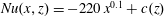 $Nu(x,z)=-220\,x^{0.1}+c(z)$
, where
$Nu(x,z)=-220\,x^{0.1}+c(z)$
, where
 $c(z)$
varies from
$c(z)$
varies from
 $727$
in the centre over
$727$
in the centre over
 $739$
and
$739$
and
 $748$
to
$748$
to
 $789$
close to the lateral wall.
$789$
close to the lateral wall.
The secondary flow structures enhance the mixing of hot and cold fluid and consequently increase the heat transport away from the heated wall into the duct core. Figure 16 depicts the heat transfer distribution via the Nusselt number varying in the streamwise and spanwise directions due to the effect of the corner vortices. The two small vortices above the bottom wall, indicated in figure 16(a) with their respective rotating direction, produce a significant spanwise gradient in the heat transfer. By transporting hot fluid into the duct centre and together with the larger vortices pushing cold fluid into the corner, the secondary flow increases the temperature gradient in the corner area and reduces it at the duct centre. The heat transfer characterised by the Nusselt number
 $Nu(x,z)$
calculated following equation (3.1) varies for the considered section from
$Nu(x,z)$
calculated following equation (3.1) varies for the considered section from
 ${\approx}410$
in the corner to
${\approx}410$
in the corner to
 ${\approx}350$
at the duct centre. Additionally a streamwise Nusselt number variation is present. The degradation of the heat transfer along the entire duct length can be seen in figure 16(b). The distribution is typical for a thermal entrance problem. After a short initial phase, where the highest temperature gradients are present and the strongest heat transfer occurs, the Nusselt number at all considered spanwise locations decreases following a power law of the form
${\approx}350$
at the duct centre. Additionally a streamwise Nusselt number variation is present. The degradation of the heat transfer along the entire duct length can be seen in figure 16(b). The distribution is typical for a thermal entrance problem. After a short initial phase, where the highest temperature gradients are present and the strongest heat transfer occurs, the Nusselt number at all considered spanwise locations decreases following a power law of the form
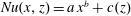 $Nu(x,z)=a\,x^{b}+c(z)$
, where in our case
$Nu(x,z)=a\,x^{b}+c(z)$
, where in our case
 $a=-220$
,
$a=-220$
,
 $b=0.1$
and
$b=0.1$
and
 $c(z)$
varies in the spanwise direction, see figure 16. Due to the continuous mixing of hot fluid at the heated wall with cold fluid in the duct core, the heat flux remains relatively high, however, it drops steadily in the streamwise direction. Averaging the local Nusselt number distribution in the spanwise and streamwise direction results in a mean value
$c(z)$
varies in the spanwise direction, see figure 16. Due to the continuous mixing of hot fluid at the heated wall with cold fluid in the duct core, the heat flux remains relatively high, however, it drops steadily in the streamwise direction. Averaging the local Nusselt number distribution in the spanwise and streamwise direction results in a mean value
 $Nu_{xz}$
for the investigated configuration of
$Nu_{xz}$
for the investigated configuration of
 $Nu_{xz}=370.7$
.
$Nu_{xz}=370.7$
.
The turbulent Prandtl number
 $Pr_{t}$
is defined as the ratio of turbulent eddy viscosity and turbulent eddy thermal diffusivity,
$Pr_{t}$
is defined as the ratio of turbulent eddy viscosity and turbulent eddy thermal diffusivity,
 $Pr_{t}=\unicode[STIX]{x1D708}_{t}/\unicode[STIX]{x1D6FC}_{t}$
. Often a constant value is assumed for
$Pr_{t}=\unicode[STIX]{x1D708}_{t}/\unicode[STIX]{x1D6FC}_{t}$
. Often a constant value is assumed for
 $Pr_{t}$
employing the Reynolds analogy (equal turbulent heat flux and momentum flux yielding a constant value of
$Pr_{t}$
employing the Reynolds analogy (equal turbulent heat flux and momentum flux yielding a constant value of
 $Pr_{t}=1$
) or based on experimental data, as
$Pr_{t}=1$
) or based on experimental data, as
 $Pr_{t}$
depends on the molecular Prandtl number. The latter has been used, e.g. in the heated duct studies by Salinas-Vásquez & Métais (Reference Salinas-Vásquez and Métais2002) and Hébrard et al. (Reference Hébrard, Salinas-Vásquez and Métais2005), in which
$Pr_{t}$
depends on the molecular Prandtl number. The latter has been used, e.g. in the heated duct studies by Salinas-Vásquez & Métais (Reference Salinas-Vásquez and Métais2002) and Hébrard et al. (Reference Hébrard, Salinas-Vásquez and Métais2005), in which
 $Pr_{t}$
is set to
$Pr_{t}$
is set to
 $0.6$
. An extensive overview of available experimental data is given by Kays (Reference Kays1994).
$0.6$
. An extensive overview of available experimental data is given by Kays (Reference Kays1994).

Figure 17. Distribution of the angles
 $\unicode[STIX]{x1D711}_{M}$
and
$\unicode[STIX]{x1D711}_{M}$
and
 $\unicode[STIX]{x1D711}_{H}$
in the lower half of the heated duct cross-section at a streamwise location of
$\unicode[STIX]{x1D711}_{H}$
in the lower half of the heated duct cross-section at a streamwise location of
 $595~\text{mm}$
, see equation (5.2) for the angle definition. Streamwise averaging is performed over
$595~\text{mm}$
, see equation (5.2) for the angle definition. Streamwise averaging is performed over
 $10~\text{mm}$
and the duct symmetry is utilised. The contour lines are drawn in steps of
$10~\text{mm}$
and the duct symmetry is utilised. The contour lines are drawn in steps of
 $1^{\circ }$
.
$1^{\circ }$
.
For a TBL with the
 $x$
-axis marking the streamwise and the
$x$
-axis marking the streamwise and the
 $y$
-axis the wall-normal direction, the eddy viscosity is defined as
$y$
-axis the wall-normal direction, the eddy viscosity is defined as
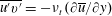 $\overline{u^{\prime }v^{\prime }}=-\unicode[STIX]{x1D708}_{t}\,(\unicode[STIX]{x2202}\overline{u}/\unicode[STIX]{x2202}y)$
and the eddy thermal diffusivity as
$\overline{u^{\prime }v^{\prime }}=-\unicode[STIX]{x1D708}_{t}\,(\unicode[STIX]{x2202}\overline{u}/\unicode[STIX]{x2202}y)$
and the eddy thermal diffusivity as
 $\overline{T^{\prime }v^{\prime }}=-\unicode[STIX]{x1D6FC}_{t}\,(\unicode[STIX]{x2202}\overline{T}/\unicode[STIX]{x2202}y)$
. This definition has also been applied for more complex configurations, e.g. for a mixed convection set-up consisting of an asymmetrically heated channel and a heated cylinder slightly above the heated wall (Kang & Iaccarino Reference Kang and Iaccarino2010) and an symmetrically heated square duct flow (Hirota et al.
Reference Hirota, Fujita, Yokosawa, Nakai and Itoh1997). For our case, however, we observed that this definition is unsuitable to analyse the cross-sectional
$\overline{T^{\prime }v^{\prime }}=-\unicode[STIX]{x1D6FC}_{t}\,(\unicode[STIX]{x2202}\overline{T}/\unicode[STIX]{x2202}y)$
. This definition has also been applied for more complex configurations, e.g. for a mixed convection set-up consisting of an asymmetrically heated channel and a heated cylinder slightly above the heated wall (Kang & Iaccarino Reference Kang and Iaccarino2010) and an symmetrically heated square duct flow (Hirota et al.
Reference Hirota, Fujita, Yokosawa, Nakai and Itoh1997). For our case, however, we observed that this definition is unsuitable to analyse the cross-sectional
 $Pr_{t}$
-distribution due to the additional lateral walls and especially the secondary flow influence. Hence, we introduce a new turbulent Prandtl number formulation taking both the heated as well as the adiabatic lateral wall boundary layers into account at every point of the cross-section flow field. We define the vectors
$Pr_{t}$
-distribution due to the additional lateral walls and especially the secondary flow influence. Hence, we introduce a new turbulent Prandtl number formulation taking both the heated as well as the adiabatic lateral wall boundary layers into account at every point of the cross-section flow field. We define the vectors
 $$\begin{eqnarray}\displaystyle \boldsymbol{v}_{\unicode[STIX]{x1D708}_{t},corr}=\left[\begin{array}{@{}c@{}}\overline{u^{\prime }v^{\prime }}\\ \overline{u^{\prime }w^{\prime }}\end{array}\right],\quad \boldsymbol{v}_{\unicode[STIX]{x1D708}_{t},\unicode[STIX]{x1D735}}=-\!\left[\begin{array}{@{}c@{}}\unicode[STIX]{x2202}\overline{u}/\unicode[STIX]{x2202}y\\ \unicode[STIX]{x2202}\overline{u}/\unicode[STIX]{x2202}z\end{array}\right],\quad \boldsymbol{v}_{\unicode[STIX]{x1D6FC}_{t},corr}=\left[\begin{array}{@{}c@{}}\overline{T^{\prime }v^{\prime }}\\ \overline{T^{\prime }w^{\prime }}\end{array}\right],\quad \boldsymbol{v}_{\unicode[STIX]{x1D6FC}_{t},\unicode[STIX]{x1D735}}=-\!\left[\begin{array}{@{}c@{}}\unicode[STIX]{x2202}\overline{T}/\unicode[STIX]{x2202}y\\ \unicode[STIX]{x2202}\overline{T}/\unicode[STIX]{x2202}z\end{array}\right]. & & \displaystyle \nonumber\\ \displaystyle & & \displaystyle\end{eqnarray}$$
The angles between the flux and gradient vectors are
 $$\begin{eqnarray}\displaystyle \unicode[STIX]{x1D711}_{M}=\arccos \left(\frac{\boldsymbol{v}_{\unicode[STIX]{x1D708}_{t},corr}\boldsymbol{\cdot }\boldsymbol{v}_{\unicode[STIX]{x1D708}_{t},\unicode[STIX]{x1D735}}}{|\boldsymbol{v}_{\unicode[STIX]{x1D708}_{t},corr}|\boldsymbol{\cdot }|\boldsymbol{v}_{\unicode[STIX]{x1D708}_{t},\unicode[STIX]{x1D735}}|}\right),\quad \unicode[STIX]{x1D711}_{H}=\arccos \left(\frac{\boldsymbol{v}_{\unicode[STIX]{x1D6FC}_{t},corr}\boldsymbol{\cdot }\boldsymbol{v}_{\unicode[STIX]{x1D6FC}_{t},\unicode[STIX]{x1D735}}}{|\boldsymbol{v}_{\unicode[STIX]{x1D6FC}_{t},corr}|\boldsymbol{\cdot }|\boldsymbol{v}_{\unicode[STIX]{x1D6FC}_{t},\unicode[STIX]{x1D735}}|}\right). & & \displaystyle\end{eqnarray}$$
If the angles between the correlation vectors
 $\boldsymbol{v}_{\unicode[STIX]{x1D708}_{t},corr}$
and
$\boldsymbol{v}_{\unicode[STIX]{x1D708}_{t},corr}$
and
 $\boldsymbol{v}_{\unicode[STIX]{x1D6FC}_{t},corr}$
, and the mean gradient vectors
$\boldsymbol{v}_{\unicode[STIX]{x1D6FC}_{t},corr}$
, and the mean gradient vectors
 $\boldsymbol{v}_{\unicode[STIX]{x1D708}_{t},\unicode[STIX]{x1D735}}$
and
$\boldsymbol{v}_{\unicode[STIX]{x1D708}_{t},\unicode[STIX]{x1D735}}$
and
 $\boldsymbol{v}_{\unicode[STIX]{x1D6FC}_{t},\unicode[STIX]{x1D735}}$
are zero,
$\boldsymbol{v}_{\unicode[STIX]{x1D6FC}_{t},\unicode[STIX]{x1D735}}$
are zero,
 $\unicode[STIX]{x1D708}_{t}$
and
$\unicode[STIX]{x1D708}_{t}$
and
 $\unicode[STIX]{x1D6FC}_{t}$
can be calculated using the TBL formulation. In this case, the Boussinesq turbulent viscosity hypothesis is valid. The cross-sectional distributions of the angles defined by equation (5.2) are shown in figure 17. We observe that in the regions influenced by the corner vortices both the values for
$\unicode[STIX]{x1D6FC}_{t}$
can be calculated using the TBL formulation. In this case, the Boussinesq turbulent viscosity hypothesis is valid. The cross-sectional distributions of the angles defined by equation (5.2) are shown in figure 17. We observe that in the regions influenced by the corner vortices both the values for
 $\unicode[STIX]{x1D711}_{M}$
as well as
$\unicode[STIX]{x1D711}_{M}$
as well as
 $\unicode[STIX]{x1D711}_{H}$
differ significantly from zero. Hence, turbulence models based on an isotropic eddy viscosity and diffusivity are invalid. Nevertheless, we can employ the least square method to determine the optimum eddy viscosity
$\unicode[STIX]{x1D711}_{H}$
differ significantly from zero. Hence, turbulence models based on an isotropic eddy viscosity and diffusivity are invalid. Nevertheless, we can employ the least square method to determine the optimum eddy viscosity
 $\unicode[STIX]{x1D708}_{t}$
and eddy diffusivity
$\unicode[STIX]{x1D708}_{t}$
and eddy diffusivity
 $\unicode[STIX]{x1D6FC}_{t}$
at a specific location in the cross-section. This leads to the definitions
$\unicode[STIX]{x1D6FC}_{t}$
at a specific location in the cross-section. This leads to the definitions
 $$\begin{eqnarray}\displaystyle \unicode[STIX]{x1D708}_{t}=\frac{\boldsymbol{v}_{\unicode[STIX]{x1D708}_{t},corr}\boldsymbol{\cdot }\boldsymbol{v}_{\unicode[STIX]{x1D708}_{t},\unicode[STIX]{x1D735}}}{|\boldsymbol{v}_{\unicode[STIX]{x1D708}_{t},\unicode[STIX]{x1D735}}|^{2}},\quad \unicode[STIX]{x1D6FC}_{t}=\frac{\boldsymbol{v}_{\unicode[STIX]{x1D6FC}_{t},corr}\boldsymbol{\cdot }\boldsymbol{v}_{\unicode[STIX]{x1D6FC}_{t},\unicode[STIX]{x1D735}}}{|\boldsymbol{v}_{\unicode[STIX]{x1D6FC}_{t},\unicode[STIX]{x1D735}}|^{2}}. & & \displaystyle\end{eqnarray}$$

Figure 18. Turbulent Prandtl number distribution in the lower half of the heated duct cross-section at streamwise locations of (a)
 $x=25~\text{mm}$
, (b)
$x=25~\text{mm}$
, (b)
 $x=50~\text{mm}$
, (c)
$x=50~\text{mm}$
, (c)
 $x=100~\text{mm}$
and (d)
$x=100~\text{mm}$
and (d)
 $x=595~\text{mm}$
. Streamwise averaging is performed over
$x=595~\text{mm}$
. Streamwise averaging is performed over
 $10~\text{mm}$
and the duct symmetry is utilised.
$10~\text{mm}$
and the duct symmetry is utilised.
 $Pr_{t}$
is calculated where
$Pr_{t}$
is calculated where
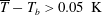 $\overline{T}-T_{b}>0.05~\text{K}$
and the contour lines are drawn in steps of
$\overline{T}-T_{b}>0.05~\text{K}$
and the contour lines are drawn in steps of
 $0.1$
.
$0.1$
.
Figure 18 shows the development of the cross-sectional turbulent Prandtl number distribution along the heated duct for the regions where the local heating surpasses a threshold value of
 $\overline{T}-T_{b}=0.05~\text{K}$
. The value range of
$\overline{T}-T_{b}=0.05~\text{K}$
. The value range of
 $Pr_{t}$
is between approximately
$Pr_{t}$
is between approximately
 $0$
and
$0$
and
 $1.3$
in figure 18, which is in good agreement with data available in the literature, e.g. with Kang & Iaccarino (Reference Kang and Iaccarino2010) using liquid water at a lower temperature, but at a similar temperature difference
$1.3$
in figure 18, which is in good agreement with data available in the literature, e.g. with Kang & Iaccarino (Reference Kang and Iaccarino2010) using liquid water at a lower temperature, but at a similar temperature difference
 $T_{w}-T_{b}$
.
$T_{w}-T_{b}$
.
Now we focus on the
 $Pr_{t}$
-distribution in the duct end cross-section, figure 18(d). In the heated wall centre directly at the wall
$Pr_{t}$
-distribution in the duct end cross-section, figure 18(d). In the heated wall centre directly at the wall
 $Pr_{t}$
is
$Pr_{t}$
is
 ${\approx}0.89$
. Above the heated wall, we observe a dome-shaped region of enhanced turbulent Prandtl number coinciding with the influence region of the two smaller corner vortices. Hence, we attribute this increase to the mixing by the secondary flow. A local maximum is located in the centre of this region, where the interaction of the small corner vortices leads to a strong upwards flow, with
${\approx}0.89$
. Above the heated wall, we observe a dome-shaped region of enhanced turbulent Prandtl number coinciding with the influence region of the two smaller corner vortices. Hence, we attribute this increase to the mixing by the secondary flow. A local maximum is located in the centre of this region, where the interaction of the small corner vortices leads to a strong upwards flow, with
 $Pr_{t}$
reaching
$Pr_{t}$
reaching
 ${\approx}1.06$
. This maximum is located slightly below the maximum
${\approx}1.06$
. This maximum is located slightly below the maximum
 $\overline{v}$
-velocity. The dome-shaped area is bordered by the interaction zone of the small and the respective large corner vortex both pushing fluid into the duct corner. There
$\overline{v}$
-velocity. The dome-shaped area is bordered by the interaction zone of the small and the respective large corner vortex both pushing fluid into the duct corner. There
 $Pr_{t}$
drops to values between
$Pr_{t}$
drops to values between
 ${\approx}0.9$
and
${\approx}0.9$
and
 ${\approx}0.95$
. The mixing of the large corner vortices also leads to an area of enhanced turbulent Prandtl number. However, due to the proximity of the adiabatic walls the
${\approx}0.95$
. The mixing of the large corner vortices also leads to an area of enhanced turbulent Prandtl number. However, due to the proximity of the adiabatic walls the
 $Pr_{t}$
-levels are lower than in the small vortex influence zone. In the core of the large vortex,
$Pr_{t}$
-levels are lower than in the small vortex influence zone. In the core of the large vortex,
 $Pr_{t}$
reaches
$Pr_{t}$
reaches
 ${\approx}0.84$
versus
${\approx}0.84$
versus
 $Pr_{t}\approx 0.94$
in the core of the small vortex. Along the lateral side walls
$Pr_{t}\approx 0.94$
in the core of the small vortex. Along the lateral side walls
 $\unicode[STIX]{x1D6FC}_{t}$
is two orders of magnitude larger than
$\unicode[STIX]{x1D6FC}_{t}$
is two orders of magnitude larger than
 $\unicode[STIX]{x1D708}_{t}$
leading to a turbulent Prandtl number of almost zero, which is a consequence of the adiabatic wall boundary condition. Depending on the
$\unicode[STIX]{x1D708}_{t}$
leading to a turbulent Prandtl number of almost zero, which is a consequence of the adiabatic wall boundary condition. Depending on the
 $y$
-location,
$y$
-location,
 $Pr_{t}$
increases steadily in the spanwise direction towards the
$Pr_{t}$
increases steadily in the spanwise direction towards the
 $z=0$
centre line until either the small or the large vortex influence region is reached, or for
$z=0$
centre line until either the small or the large vortex influence region is reached, or for
 $2y/Ly>0.7$
a narrow maximum region located along the centre line. There, the global maximum is reached with
$2y/Ly>0.7$
a narrow maximum region located along the centre line. There, the global maximum is reached with
 $Pr_{t}=1.3$
located slightly above the minimum
$Pr_{t}=1.3$
located slightly above the minimum
 $\overline{v}$
-velocity in the interaction zone of the large vortices.
$\overline{v}$
-velocity in the interaction zone of the large vortices.
Along the duct length, i.e. from figure 18(a–d), the turbulent Prandtl number levels in the vicinity of the heated wall drop continuously. The maximum values within the dome-shaped region decrease from
 $1.28$
at
$1.28$
at
 $x=25~\text{mm}$
over
$x=25~\text{mm}$
over
 $1.16$
at
$1.16$
at
 $x=50~\text{mm}$
and
$x=50~\text{mm}$
and
 $1.11$
at
$1.11$
at
 $x=100~\text{mm}$
to
$x=100~\text{mm}$
to
 $1.06$
at
$1.06$
at
 $x=595~\text{mm}$
. Also the maximum location moves slightly closer towards the heated wall. Close to the lateral wall, the variations in the streamwise direction are smaller compared to those in the centre as this location is strongly influenced by the adiabatic wall boundary layer.
$x=595~\text{mm}$
. Also the maximum location moves slightly closer towards the heated wall. Close to the lateral wall, the variations in the streamwise direction are smaller compared to those in the centre as this location is strongly influenced by the adiabatic wall boundary layer.
Based on the
 $Pr_{t}$
-distributions we conclude that the assumption of a constant value for the turbulent Prandtl number for asymmetrically heated duct flows is invalid.
$Pr_{t}$
-distributions we conclude that the assumption of a constant value for the turbulent Prandtl number for asymmetrically heated duct flows is invalid.
5.4 Turbulence anisotropy
In the following we will further analyse the influence of wall heating on turbulence anisotropy as the secondary flow is a consequence of the Reynolds stress anisotropy. For this investigation we apply the anisotropy-invariant map (AIM) and the barycentric anisotropy map (BAM), see Emory & Iaccarino (Reference Emory and Iaccarino2014) for an overview.

Figure 19. Reynolds stress anisotropy-invariant map for the adiabatic duct (——) and the heated duct (——, orange) evaluated at (a,b)
 $2z/L_{z}=0$
and (c,d)
$2z/L_{z}=0$
and (c,d)
 $2z/L_{z}=0.95$
along the
$2z/L_{z}=0.95$
along the
 $y$
-line from the heated wall to the duct centre, and limiting states defined by the Lumley triangle. The wall location is represented by ● and ● (orange) respectively.
$y$
-line from the heated wall to the duct centre, and limiting states defined by the Lumley triangle. The wall location is represented by ● and ● (orange) respectively.
The Reynolds stress anisotropy tensor is defined as
 $\unicode[STIX]{x1D622}_{ij}=\overline{u_{i}^{\prime }u_{j}^{\prime }}/(2k)-\unicode[STIX]{x1D6FF}_{ij}/3$
with the turbulent kinetic energy being
$\unicode[STIX]{x1D622}_{ij}=\overline{u_{i}^{\prime }u_{j}^{\prime }}/(2k)-\unicode[STIX]{x1D6FF}_{ij}/3$
with the turbulent kinetic energy being
 $k=\overline{u_{n}^{\prime }u_{n}^{\prime }}/2$
and
$k=\overline{u_{n}^{\prime }u_{n}^{\prime }}/2$
and
 $\unicode[STIX]{x1D6FF}_{ij}$
the Kronecker delta. Three limit states are defined forming the vertices of the so-called Lumley triangle: the state of 1-component turbulence, for which turbulent fluctuations in one direction are dominant, the state of 2-component turbulence, for which turbulent fluctuations in two directions are much higher than in the third direction, and the state of 3-component isotropic turbulence, where fluctuations in all directions are equally high (Lumley Reference Lumley1978; Choi & Lumley Reference Choi and Lumley2001). Any anisotropy state
$\unicode[STIX]{x1D6FF}_{ij}$
the Kronecker delta. Three limit states are defined forming the vertices of the so-called Lumley triangle: the state of 1-component turbulence, for which turbulent fluctuations in one direction are dominant, the state of 2-component turbulence, for which turbulent fluctuations in two directions are much higher than in the third direction, and the state of 3-component isotropic turbulence, where fluctuations in all directions are equally high (Lumley Reference Lumley1978; Choi & Lumley Reference Choi and Lumley2001). Any anisotropy state
 $\unicode[STIX]{x1D622}_{ij}$
can be described as convex combination of these three limiting states, i.e. every realisable state has to reside within the borders of the Lumley triangle. The construction of the AIM is based on the anisotropy tensor eigenvalues
$\unicode[STIX]{x1D622}_{ij}$
can be described as convex combination of these three limiting states, i.e. every realisable state has to reside within the borders of the Lumley triangle. The construction of the AIM is based on the anisotropy tensor eigenvalues
 $\unicode[STIX]{x1D706}_{i}$
. The two axes are the second and third invariants of the anisotropy tensor with
$\unicode[STIX]{x1D706}_{i}$
. The two axes are the second and third invariants of the anisotropy tensor with
 $I_{2}=\unicode[STIX]{x1D622}_{ij}\unicode[STIX]{x1D622}_{ji}/2=\unicode[STIX]{x1D706}_{1}^{2}+\unicode[STIX]{x1D706}_{1}\unicode[STIX]{x1D706}_{2}+\unicode[STIX]{x1D706}_{2}^{2}$
and
$I_{2}=\unicode[STIX]{x1D622}_{ij}\unicode[STIX]{x1D622}_{ji}/2=\unicode[STIX]{x1D706}_{1}^{2}+\unicode[STIX]{x1D706}_{1}\unicode[STIX]{x1D706}_{2}+\unicode[STIX]{x1D706}_{2}^{2}$
and
 $I_{3}=\unicode[STIX]{x1D622}_{ij}\unicode[STIX]{x1D622}_{jn}\unicode[STIX]{x1D622}_{ni}/3=-\unicode[STIX]{x1D706}_{1}\unicode[STIX]{x1D706}_{2}(\unicode[STIX]{x1D706}_{1}+\unicode[STIX]{x1D706}_{2})$
respectively. The location of a certain turbulence state in the AIM then describes the shape of the Reynolds stress tensor, see Simonsen & Krogstad (Reference Simonsen and Krogstad2005).
$I_{3}=\unicode[STIX]{x1D622}_{ij}\unicode[STIX]{x1D622}_{jn}\unicode[STIX]{x1D622}_{ni}/3=-\unicode[STIX]{x1D706}_{1}\unicode[STIX]{x1D706}_{2}(\unicode[STIX]{x1D706}_{1}+\unicode[STIX]{x1D706}_{2})$
respectively. The location of a certain turbulence state in the AIM then describes the shape of the Reynolds stress tensor, see Simonsen & Krogstad (Reference Simonsen and Krogstad2005).
Figure 19 presents the AIM evaluated at two spanwise locations at
 $z=0$
in the duct midplane and at
$z=0$
in the duct midplane and at
 $2z/L_{z}=0.95$
close to the lateral wall. The AIM describes the evolution of the turbulence anisotropy along the
$2z/L_{z}=0.95$
close to the lateral wall. The AIM describes the evolution of the turbulence anisotropy along the
 $y$
-direction starting at the heated wall and ending at the duct centre line for the heated and the adiabatic case. For the duct midplane in figure 19(a,b) the anisotropy development resembles that of a plane channel or boundary layer flow, cf. Banerjee et al. (Reference Banerjee, Krahl, Durst and Zenger2007) and Pasquariello et al. (Reference Pasquariello, Grilli, Hickel and Adams2014). The trajectory starts at the 2-component limit edge and moves upwards in direction of the 1-component limit until the maximum anisotropy is reached in the buffer layer at
$y$
-direction starting at the heated wall and ending at the duct centre line for the heated and the adiabatic case. For the duct midplane in figure 19(a,b) the anisotropy development resembles that of a plane channel or boundary layer flow, cf. Banerjee et al. (Reference Banerjee, Krahl, Durst and Zenger2007) and Pasquariello et al. (Reference Pasquariello, Grilli, Hickel and Adams2014). The trajectory starts at the 2-component limit edge and moves upwards in direction of the 1-component limit until the maximum anisotropy is reached in the buffer layer at
 $y^{+}=6.4$
for the adiabatic case. The trajectory then turns and follows a path parallel to the axisymmetric expansion limit until a kink in the log layer. Finally a state close to isotropic turbulence is reached at the duct symmetry line. For the second location at
$y^{+}=6.4$
for the adiabatic case. The trajectory then turns and follows a path parallel to the axisymmetric expansion limit until a kink in the log layer. Finally a state close to isotropic turbulence is reached at the duct symmetry line. For the second location at
 $2z/L_{z}=0.95$
, figure 19(c,d) shows an overall similar behaviour, but also the significant influence of the lateral wall. The trajectory starts closer to the 2-component axisymmetric limit and moves upwards to the 1-component limit. In contrast to the duct centre trajectory, the off-centre trajectory follows a steeper path than the axisymmetric expansion curve after the turning point, no kink exists in the log layer and in the duct centre the state of isotropic turbulence is not reached.
$2z/L_{z}=0.95$
, figure 19(c,d) shows an overall similar behaviour, but also the significant influence of the lateral wall. The trajectory starts closer to the 2-component axisymmetric limit and moves upwards to the 1-component limit. In contrast to the duct centre trajectory, the off-centre trajectory follows a steeper path than the axisymmetric expansion curve after the turning point, no kink exists in the log layer and in the duct centre the state of isotropic turbulence is not reached.

Figure 20. Distribution of (a) diagonal components and (b) off-diagonal component
 $\overline{a_{xy}}$
of the Reynolds stress anisotropy tensor in the duct midplane along the heated wall-normal direction for the adiabatic (——) and the heated duct (——, orange).
$\overline{a_{xy}}$
of the Reynolds stress anisotropy tensor in the duct midplane along the heated wall-normal direction for the adiabatic (——) and the heated duct (——, orange).
The effect of wall heating on turbulence anisotropy is overall relatively small, restricted to the vicinity of the heated wall and more pronounced close to the lateral wall than in the duct midplane. The start points of both trajectories lie at the 2-component limit and are shifted towards the 1-component limit compared to the adiabatic case. Within the buffer layer the heated duct trajectories follow a path slightly closer to the 2-component limit. The turning point of maximum anisotropy lies still within the buffer layer, however, it is located closer to the upper right corner of the Lumley triangle. Moreover, in figure 19(a,b) a slight change of the kink in the log layer area is visible.

Figure 21. Barycentric anisotropy map illustrating regions of 1-, 2- and 3-component turbulence with (a) lower left quadrant of the adiabatic duct, (b) zoom into the lower left corner of the adiabatic duct and (c) the same detail for the heated duct (opposite corner shown). The isolines denote a constant 3-component turbulence fraction.
As the changes due to the heating are limited to the near-wall area, we investigate the anisotropy tensor components there in detail and compare our findings qualitatively with a recent study by Patel, Boersma & Pecnik (Reference Patel, Boersma and Pecnik2016), who analysed the influence of viscosity gradients on the near-wall turbulence anisotropy of a channel flow. In figure 20 we observe the same trends as Patel et al. (Reference Patel, Boersma and Pecnik2016): the streamwise component of the Reynolds stress anisotropy tensor
 $\overline{\unicode[STIX]{x1D622}_{xx}}$
increases, and the spanwise component
$\overline{\unicode[STIX]{x1D622}_{xx}}$
increases, and the spanwise component
 $\overline{a_{zz}}$
decreases with heating applied. Patel et al. (Reference Patel, Boersma and Pecnik2016) reported, that the wall-normal component
$\overline{a_{zz}}$
decreases with heating applied. Patel et al. (Reference Patel, Boersma and Pecnik2016) reported, that the wall-normal component
 $\overline{a_{yy}}$
remains unaffected, however for our case a decrease starting within the buffer layer is visible. The normalised turbulent shear stress
$\overline{a_{yy}}$
remains unaffected, however for our case a decrease starting within the buffer layer is visible. The normalised turbulent shear stress
 $\overline{a_{xy}}$
in figure 20(b) increases, indicating an augmented momentum transfer. The off-diagonal components
$\overline{a_{xy}}$
in figure 20(b) increases, indicating an augmented momentum transfer. The off-diagonal components
 $\overline{a_{yz}}$
and
$\overline{a_{yz}}$
and
 $\overline{a_{xz}}$
are negligible in the duct midplane.
$\overline{a_{xz}}$
are negligible in the duct midplane.
In contrast to the classical AIM, the so-called barycentric map proposed by Banerjee et al. (Reference Banerjee, Krahl, Durst and Zenger2007) provides a more intuitive tool to analyse the turbulence anisotropy. The construction again is based on the eigenvalues
 $\unicode[STIX]{x1D706}_{i}$
of the Reynolds stress anisotropy tensor and relies on the fact, that any realisable turbulence state can be represented as a combination of the three limiting states of 1-, 2- and 3-component turbulence. The limiting states are now defined as the corners of an equilateral triangle with
$\unicode[STIX]{x1D706}_{i}$
of the Reynolds stress anisotropy tensor and relies on the fact, that any realisable turbulence state can be represented as a combination of the three limiting states of 1-, 2- and 3-component turbulence. The limiting states are now defined as the corners of an equilateral triangle with
 $\boldsymbol{x}_{1c}=(1,0)$
,
$\boldsymbol{x}_{1c}=(1,0)$
,
 $\boldsymbol{x}_{2c}=(0,0)$
and
$\boldsymbol{x}_{2c}=(0,0)$
and
 $\boldsymbol{x}_{3c}=(1/2,\sqrt{3}/2)$
. The coordinates of a certain turbulent state are then computed as
$\boldsymbol{x}_{3c}=(1/2,\sqrt{3}/2)$
. The coordinates of a certain turbulent state are then computed as
 $\boldsymbol{x}=C_{1c}\boldsymbol{x}_{1c}+C_{2c}\boldsymbol{x}_{2c}+C_{3c}\boldsymbol{x}_{3c}$
. In contrast to the AIM, the BAM is a linear anisotropy-invariant map, where the coordinates depend linearly on the eigenvalues with
$\boldsymbol{x}=C_{1c}\boldsymbol{x}_{1c}+C_{2c}\boldsymbol{x}_{2c}+C_{3c}\boldsymbol{x}_{3c}$
. In contrast to the AIM, the BAM is a linear anisotropy-invariant map, where the coordinates depend linearly on the eigenvalues with
 $C_{1c}=\unicode[STIX]{x1D706}_{1}-\unicode[STIX]{x1D706}_{2}$
,
$C_{1c}=\unicode[STIX]{x1D706}_{1}-\unicode[STIX]{x1D706}_{2}$
,
 $C_{2c}=2(\unicode[STIX]{x1D706}_{2}-\unicode[STIX]{x1D706}_{3})$
and
$C_{2c}=2(\unicode[STIX]{x1D706}_{2}-\unicode[STIX]{x1D706}_{3})$
and
 $C_{3c}=3\unicode[STIX]{x1D706}_{3}+1$
ensuring
$C_{3c}=3\unicode[STIX]{x1D706}_{3}+1$
ensuring
 $\sum C_{ic}=1$
. For visualisation the coefficient vector
$\sum C_{ic}=1$
. For visualisation the coefficient vector
 $C_{ic}$
is mapped to the RGB triplet. Red corresponds to 1-component, green to 2-component and blue to 3-component turbulence.
$C_{ic}$
is mapped to the RGB triplet. Red corresponds to 1-component, green to 2-component and blue to 3-component turbulence.
Figure 21(a) shows the application of the barycentric map combined with the RGB colouring for the lower left quadrant of the adiabatic duct. In the duct core the state of isotropic turbulence is almost reached, and in the vicinity of the walls a mixture of 2- and 1-component turbulence is found. As noted previously using the AIM, the 2-component turbulence transitions to 1-component turbulence in the buffer layer. In the duct corner 1-component turbulence is dominant as fluctuations perpendicular to the two walls are suppressed. The influence of the corner vortices on the turbulence anisotropy distribution is clearly visible in the
 $C_{3c}$
-isolines with the mean secondary flow transporting fluid from the isotropic core region into the duct corner following approximately the corner bisecting line.
$C_{3c}$
-isolines with the mean secondary flow transporting fluid from the isotropic core region into the duct corner following approximately the corner bisecting line.
Figure 21(b,c) show the influence of the wall heating for the duct corner region. In the vicinity of the heatable wall, we observe for the heated case a reduction of 2-component turbulence in favour of 1- and 3-component turbulence. At the adiabatic upper wall (not shown) the turbulence anisotropy remains identical for both cases. The
 $C_{3c}$
-isolines illustrate the anisotropy reduction in this region as an anisotropy measure can be defined as
$C_{3c}$
-isolines illustrate the anisotropy reduction in this region as an anisotropy measure can be defined as
 $C_{ani}=1-C_{3c}$
(Banerjee et al.
Reference Banerjee, Krahl, Durst and Zenger2007). As
$C_{ani}=1-C_{3c}$
(Banerjee et al.
Reference Banerjee, Krahl, Durst and Zenger2007). As
 $C_{3c}$
increases in the near-wall region, the flow becomes more isotropic leading to a weaker production term for streamwise vorticity and in turn to the observed weakening of the secondary flow over the duct length.
$C_{3c}$
increases in the near-wall region, the flow becomes more isotropic leading to a weaker production term for streamwise vorticity and in turn to the observed weakening of the secondary flow over the duct length.
5.5 Length scales of turbulent structures
As discussed in § 5.2, the size and strength of the ejections and streaky structures reduce with increasing temperature and the associated viscosity reduction. Salinas-Vásquez & Métais (Reference Salinas-Vásquez and Métais2002) have shown, that the ejections and streaks as well as turbulent length scales grow with increasing viscosity. Hence, we expect in our case a reduction of the turbulent length scales when heating is applied.

Figure 22. Streamwise velocity fluctuations within the heatable wall-parallel plane at
 $2y/L_{y}=0.9975$
for the adiabatic and the heated duct.
$2y/L_{y}=0.9975$
for the adiabatic and the heated duct.

Figure 23. Spanwise velocity fluctuations within the heatable wall-parallel plane at
 $2y/L_{y}=0.9975$
for the adiabatic and the heated duct.
$2y/L_{y}=0.9975$
for the adiabatic and the heated duct.
As mainly the area close to the lower wall is affected by the heating, we first analyse the turbulent length scales qualitatively on a plane parallel to and directly above the heatable wall at
 $2y/L_{y}=0.9975$
. This location corresponds to
$2y/L_{y}=0.9975$
. This location corresponds to
 $y^{+}=16.1$
for the adiabatic duct and to
$y^{+}=16.1$
for the adiabatic duct and to
 $y^{+}=24.2$
for the end section of the heated duct, where
$y^{+}=24.2$
for the end section of the heated duct, where
 $y^{+}$
is evaluated at
$y^{+}$
is evaluated at
 $2z/L_{z}=0$
. Figure 22 depicts the streamwise velocity fluctuations
$2z/L_{z}=0$
. Figure 22 depicts the streamwise velocity fluctuations
 $u^{\prime }/u_{b}$
and figure 23 the spanwise velocity fluctuations
$u^{\prime }/u_{b}$
and figure 23 the spanwise velocity fluctuations
 $w^{\prime }/u_{b}$
within this plane.
$w^{\prime }/u_{b}$
within this plane.
In figure 22, the typical streaky structures of the TBL with the darker regions of comparatively low-speed fluid surrounded by lighter regions of high-speed fluid are visible. Due to the restricting influence, the streaks close to the lateral wall, i.e. in the duct corner, are thinner and shorter compared to those in the centre. As the streak size scales with viscous thickness and based on previous studies, we expect a reduction of streak size as well as turbulent length scales in the heated duct (Salinas-Vásquez & Métais Reference Salinas-Vásquez and Métais2002; Zonta et al. Reference Zonta, Marchioli and Soldati2012; Lee et al. Reference Lee, Jung, Sung and Zaki2013). However, comparing the two snapshots, no qualitative difference in turbulent structures is visible. We make the same observation for the spanwise fluctuations in figure 23, which we attribute to the moderate heating.

Figure 24. Longitudinal autocorrelations of streamwise velocity
 $R_{uu}^{x}$
at different locations marked in the sketches on the respective right-hand side. In (a) the adiabatic duct results are shown and in (b) the change due to the viscosity modulation. Heated duct correlations are coloured orange and the ones at off-centre locations blue. The line
$R_{uu}^{x}$
at different locations marked in the sketches on the respective right-hand side. In (a) the adiabatic duct results are shown and in (b) the change due to the viscosity modulation. Heated duct correlations are coloured orange and the ones at off-centre locations blue. The line
 $R_{uu}^{x}=1/\text{e}^{2}$
(——, grey) is used to determine
$R_{uu}^{x}=1/\text{e}^{2}$
(——, grey) is used to determine
 $r_{lim,x}$
. For figure legend and line parameters see table 4.
$r_{lim,x}$
. For figure legend and line parameters see table 4.
The use of autocorrelations allows for a quantitative investigation of turbulent length scales and their respective changes. To reduce the number of samples required for a converged result, we assume local homogeneity in the streamwise direction for the definition of the longitudinal autocorrelation function of the
 $u$
-velocity
$u$
-velocity
 $R_{uu}^{x}$
(Pirozzoli, Grasso & Gatski Reference Pirozzoli, Grasso and Gatski2004). The sampling rate is every
$R_{uu}^{x}$
(Pirozzoli, Grasso & Gatski Reference Pirozzoli, Grasso and Gatski2004). The sampling rate is every
 $25$
time steps over a sampling period of
$25$
time steps over a sampling period of
 $20$
FTT with respect to
$20$
FTT with respect to
 $L_{x,heat}$
, leading to a total of
$L_{x,heat}$
, leading to a total of
 ${\approx}56.7\times 10^{3}$
samples. The integral length scale is generally defined as
${\approx}56.7\times 10^{3}$
samples. The integral length scale is generally defined as
 $L_{ii}^{j}=\int _{0}^{\infty }R_{ii}^{j}(r_{j})\,\text{d}r_{j}$
. For the upper bound of integration, a finite value
$L_{ii}^{j}=\int _{0}^{\infty }R_{ii}^{j}(r_{j})\,\text{d}r_{j}$
. For the upper bound of integration, a finite value
 $r_{lim,j}$
has to be specified. O’Neill et al. (Reference O’Neill, Nicolaides, Honnery, Soria, Behnia, Lin and McBain2004) proposed the integration up to the first zero crossing of the correlation or until the correlation function has fallen to a value of
$r_{lim,j}$
has to be specified. O’Neill et al. (Reference O’Neill, Nicolaides, Honnery, Soria, Behnia, Lin and McBain2004) proposed the integration up to the first zero crossing of the correlation or until the correlation function has fallen to a value of
 $1/\text{e}$
. As the latter cuts off a large part of the correlation function, it tends to underestimate the turbulent length scale. Hence we use a limit of
$1/\text{e}$
. As the latter cuts off a large part of the correlation function, it tends to underestimate the turbulent length scale. Hence we use a limit of
 $1/\text{e}^{2}$
, so that
$1/\text{e}^{2}$
, so that
 $r_{lim,j}$
is defined as
$r_{lim,j}$
is defined as
 $r_{lim,j}=r_{j}(R_{ii}^{j}=1/\text{e}^{2})$
.
$r_{lim,j}=r_{j}(R_{ii}^{j}=1/\text{e}^{2})$
.
Figure 24 shows the longitudinal autocorrelation functions
 $R_{uu}^{x}$
at different (
$R_{uu}^{x}$
at different (
 $y/z$
)-positions for the heated and adiabatic duct. All positions are located in the vicinity of the heatable wall, i.e. in the area influenced by the small corner vortices except
$y/z$
)-positions for the heated and adiabatic duct. All positions are located in the vicinity of the heatable wall, i.e. in the area influenced by the small corner vortices except
 $R_{uu,7}^{x}$
, which lies in the area influenced by the larger corner vortices, see table 4 for line parameters and turbulent length scales. Figure 24(a) allows for two observations: first the trivial result, that with increasing distance from the heatable wall the turbulent structures grow larger with diminishing growth rate for each
$R_{uu,7}^{x}$
, which lies in the area influenced by the larger corner vortices, see table 4 for line parameters and turbulent length scales. Figure 24(a) allows for two observations: first the trivial result, that with increasing distance from the heatable wall the turbulent structures grow larger with diminishing growth rate for each
 $R_{uu}^{x}$
-curve, except for
$R_{uu}^{x}$
-curve, except for
 $R_{uu,7}^{x}$
at
$R_{uu,7}^{x}$
at
 $2y/L_{y}\approx -0.8$
, where a reduction in turbulent length scale is apparent. Second, the structures become significantly smaller when moving in the direction of the duct corner due to the increasing influence of the lateral wall. Comparing the turbulent length scales in the plane shown in figure 22 for the duct centre position
$2y/L_{y}\approx -0.8$
, where a reduction in turbulent length scale is apparent. Second, the structures become significantly smaller when moving in the direction of the duct corner due to the increasing influence of the lateral wall. Comparing the turbulent length scales in the plane shown in figure 22 for the duct centre position
 $R_{uu,1}^{x}$
with the two off-centre positions
$R_{uu,1}^{x}$
with the two off-centre positions
 $R_{uu,1a}^{x}$
and
$R_{uu,1a}^{x}$
and
 $R_{uu,1b}^{x}$
, we measure a reduction of
$R_{uu,1b}^{x}$
, we measure a reduction of
 $-15.0\,\%$
and
$-15.0\,\%$
and
 $-34.7\,\%$
respectively. Further away from the lower wall the
$-34.7\,\%$
respectively. Further away from the lower wall the
 $2y/L_{y}=\text{const.}$
correlation triplets follow the same trend.
$2y/L_{y}=\text{const.}$
correlation triplets follow the same trend.
In figure 24(b) we investigate the influence of the viscosity modulation on turbulent length scales
 $L_{uu}^{x}$
. We observe the expected heating-induced shortening for all considered locations. As the temperature increase is highest directly at the lower wall, we observe a strong reduction there with a maximum value of
$L_{uu}^{x}$
. We observe the expected heating-induced shortening for all considered locations. As the temperature increase is highest directly at the lower wall, we observe a strong reduction there with a maximum value of
 $-10.2\,\%$
for
$-10.2\,\%$
for
 $y^{+}=16.1$
. Moving upwards along the duct midplane, the reduction in the small corner vortex region becomes increasingly weak, see table 4. For instance at
$y^{+}=16.1$
. Moving upwards along the duct midplane, the reduction in the small corner vortex region becomes increasingly weak, see table 4. For instance at
 $2y/L_{y}\approx -0.9$
, the shortening has fallen to just
$2y/L_{y}\approx -0.9$
, the shortening has fallen to just
 $-1.6\,\%$
. However, the viscosity effect on turbulent length scales does not only affect the immediate vicinity of the heated wall, but also the duct centre due to the modified secondary flow transport. This becomes apparent by comparison of
$-1.6\,\%$
. However, the viscosity effect on turbulent length scales does not only affect the immediate vicinity of the heated wall, but also the duct centre due to the modified secondary flow transport. This becomes apparent by comparison of
 $R_{uu,6}^{x}$
and
$R_{uu,6}^{x}$
and
 $R_{uu,7}^{x}$
, where the first is in the influence region of the small corner vortices and the latter in that of the large corner vortices. At
$R_{uu,7}^{x}$
, where the first is in the influence region of the small corner vortices and the latter in that of the large corner vortices. At
 $2y/L_{y}\approx -0.9$
, the viscosity drop is approximately twice as much as at
$2y/L_{y}\approx -0.9$
, the viscosity drop is approximately twice as much as at
 $2y/L_{y}\approx -0.8$
, but the length scale reduction increases from
$2y/L_{y}\approx -0.8$
, but the length scale reduction increases from
 $-1.6\,\%$
for
$-1.6\,\%$
for
 $R_{uu,6}^{x}$
to even
$R_{uu,6}^{x}$
to even
 $-14.8\,\%$
for
$-14.8\,\%$
for
 $R_{uu,7}^{x}$
. Thus, the reduction of turbulent length scales is not a mere function of temperature increase, but depends on the specific location as the viscosity modulation affects turbulent transport as well as the transport by secondary flows and both influence
$R_{uu,7}^{x}$
. Thus, the reduction of turbulent length scales is not a mere function of temperature increase, but depends on the specific location as the viscosity modulation affects turbulent transport as well as the transport by secondary flows and both influence
 $L_{uu}^{x}$
. The argument is supported by comparing the off-centre locations, exemplarily
$L_{uu}^{x}$
. The argument is supported by comparing the off-centre locations, exemplarily
 $R_{uu,1}^{x}$
in the centre with
$R_{uu,1}^{x}$
in the centre with
 $R_{uu,1a}^{x}$
and
$R_{uu,1a}^{x}$
and
 $R_{uu,1b}^{x}$
. The relative shortening in the centre is with
$R_{uu,1b}^{x}$
. The relative shortening in the centre is with
 $-10.2\,\%$
significantly higher than the
$-10.2\,\%$
significantly higher than the
 $-4.7\,\%$
and
$-4.7\,\%$
and
 $-4.3\,\%$
. The correlations are influenced by the small CW vortex above the heatable wall, which leads to a non-uniform viscosity drop in the spanwise direction by transporting fluid from the duct corner into the wall centre. This motion produces an increased temperature in the midplane of
$-4.3\,\%$
. The correlations are influenced by the small CW vortex above the heatable wall, which leads to a non-uniform viscosity drop in the spanwise direction by transporting fluid from the duct corner into the wall centre. This motion produces an increased temperature in the midplane of
 $19.6~\text{K}$
versus
$19.6~\text{K}$
versus
 $17.9~\text{K}$
, respectively
$17.9~\text{K}$
, respectively
 $17.6~\text{K}$
. However, the viscosity drop differs too little in the spanwise direction as to explain the large difference in length scale shortening and thus it is a secondary flow effect.
$17.6~\text{K}$
. However, the viscosity drop differs too little in the spanwise direction as to explain the large difference in length scale shortening and thus it is a secondary flow effect.
Table 4. Parameters for the longitudinal autocorrelations of streamwise velocity shown in figure 24. Listed are (
 $y/z$
)-positions, dimensionless height above the heatable wall, temperature increase, viscosity drop, integral length scales and their relative changes due to the viscosity modulation. The lengths
$y/z$
)-positions, dimensionless height above the heatable wall, temperature increase, viscosity drop, integral length scales and their relative changes due to the viscosity modulation. The lengths
 $L_{uu}^{x}$
are normalised by a factor of (
$L_{uu}^{x}$
are normalised by a factor of (
 $100\,d_{h}$
).
$100\,d_{h}$
).

Table 5. Parameters for the autocorrelations of streamwise and spanwise velocity in the spanwise direction shown in figure 25.
 $R_{ii,k,lw}^{z}$
denote the curves taken at the lateral wall and
$R_{ii,k,lw}^{z}$
denote the curves taken at the lateral wall and
 $R_{ii,k}^{z}$
the ones taken further away from it. Listed are the position of the correlations, temperature increase, viscosity drop, integral length scales and their relative changes due to the heating. All
$R_{ii,k}^{z}$
the ones taken further away from it. Listed are the position of the correlations, temperature increase, viscosity drop, integral length scales and their relative changes due to the heating. All
 $L_{ii}^{z}$
are normalised by a factor of (
$L_{ii}^{z}$
are normalised by a factor of (
 $100\,d_{h}$
).
$100\,d_{h}$
).


Figure 25. Transverse autocorrelations of streamwise velocity
 $R_{uu}^{z}$
in (a,b) and longitudinal autocorrelations of spanwise velocity
$R_{uu}^{z}$
in (a,b) and longitudinal autocorrelations of spanwise velocity
 $R_{ww}^{z}$
in (c,d) at different locations. In (a,c) the correlations at the lateral wall are shown and in (b,d) the ones at
$R_{ww}^{z}$
in (c,d) at different locations. In (a,c) the correlations at the lateral wall are shown and in (b,d) the ones at
 $2z/L_{z}=0.74$
. Results for the adiabatic duct are coloured black and for the heated duct orange. The line
$2z/L_{z}=0.74$
. Results for the adiabatic duct are coloured black and for the heated duct orange. The line
 $R_{ii}^{z}=1/\text{e}^{2}$
used to determine
$R_{ii}^{z}=1/\text{e}^{2}$
used to determine
 $r_{lim,z}$
is marked by (——, grey). For figure legend and line parameters see table 5.
$r_{lim,z}$
is marked by (——, grey). For figure legend and line parameters see table 5.
For the turbulent length scales in the spanwise direction, specifically for the transverse autocorrelations
 $R_{uu}^{z}$
and the longitudinal autocorrelations
$R_{uu}^{z}$
and the longitudinal autocorrelations
 $R_{ww}^{z}$
, data are gathered along a
$R_{ww}^{z}$
, data are gathered along a
 $z$
-line with the same sampling parameters as before and evaluated following Pope (Reference Pope2000). Additionally, a quadrant averaging is performed to utilise the symmetry with respect to the
$z$
-line with the same sampling parameters as before and evaluated following Pope (Reference Pope2000). Additionally, a quadrant averaging is performed to utilise the symmetry with respect to the
 $y$
-axis. The parameters for the correlations are listed in table 5. We first discuss the results for the adiabatic case and subsequently analyse the changes due to heat transfer at two spanwise locations. The first is directly at the lateral wall and the second further away from it at
$y$
-axis. The parameters for the correlations are listed in table 5. We first discuss the results for the adiabatic case and subsequently analyse the changes due to heat transfer at two spanwise locations. The first is directly at the lateral wall and the second further away from it at
 $2z/L_{z}=0.74$
. The latter position is chosen instead of the duct centre due to the higher
$2z/L_{z}=0.74$
. The latter position is chosen instead of the duct centre due to the higher
 $z$
-direction grid resolution.
$z$
-direction grid resolution.
In figure 25(a,b) transversal correlations of streamwise velocity in the spanwise direction
 $R_{uu}^{z}$
are depicted for different locations. Moving away from the lower wall, the structures at the lateral wall
$R_{uu}^{z}$
are depicted for different locations. Moving away from the lower wall, the structures at the lateral wall
 $L_{uu,k,lw}^{z}$
as well as the larger
$L_{uu,k,lw}^{z}$
as well as the larger
 $L_{uu,k}^{z}$
at
$L_{uu,k}^{z}$
at
 $2z/L_{z}=0.74$
increase. However, the
$2z/L_{z}=0.74$
increase. However, the
 $L_{uu,k,lw}^{z}$
become only slightly larger due to the strong influence of the lateral wall, see table 5. The longitudinal correlations
$L_{uu,k,lw}^{z}$
become only slightly larger due to the strong influence of the lateral wall, see table 5. The longitudinal correlations
 $R_{ww}^{z}$
are shown in figure 25(c,d). The
$R_{ww}^{z}$
are shown in figure 25(c,d). The
 $L_{ww,k}^{z}$
are consistently larger than the
$L_{ww,k}^{z}$
are consistently larger than the
 $L_{uu,k}^{z}$
, whereas close to the lateral wall, the
$L_{uu,k}^{z}$
, whereas close to the lateral wall, the
 $L_{ww,k,lw}^{z}$
are shorter than the
$L_{ww,k,lw}^{z}$
are shorter than the
 $L_{uu,k,lw}^{z}$
as the spanwise fluctuations are blocked by the wall. The integral length scales may serve to characterise quantitatively the structures visible in the velocity fluctuation plots at the beginning of this section, in figures 22 and 23. Qualitatively, the streaky structures are much more elongated than the structures visible in the
$L_{uu,k,lw}^{z}$
as the spanwise fluctuations are blocked by the wall. The integral length scales may serve to characterise quantitatively the structures visible in the velocity fluctuation plots at the beginning of this section, in figures 22 and 23. Qualitatively, the streaky structures are much more elongated than the structures visible in the
 $w^{\prime }$
-plot. Close to the heatable wall, corresponding to the plane shown in figures 22 and 23, and at
$w^{\prime }$
-plot. Close to the heatable wall, corresponding to the plane shown in figures 22 and 23, and at
 $2z/L_{z}=0.74$
, the ratios of integral length scales are
$2z/L_{z}=0.74$
, the ratios of integral length scales are
 $L_{uu}^{x}/L_{uu}^{z}\approx 7.6$
and
$L_{uu}^{x}/L_{uu}^{z}\approx 7.6$
and
 $L_{ww}^{x}/L_{ww}^{z}\approx 2.8$
, which supports the qualitative observation of the more elongated streaky structures.
$L_{ww}^{x}/L_{ww}^{z}\approx 2.8$
, which supports the qualitative observation of the more elongated streaky structures.
When heating is applied, we observe close to the lateral wall a significant reduction of
 $L_{uu,k,lw}^{z}$
by up to
$L_{uu,k,lw}^{z}$
by up to
 $-31.1\,\%$
and of
$-31.1\,\%$
and of
 $L_{ww,k,lw}^{z}$
by up to
$L_{ww,k,lw}^{z}$
by up to
 $-10.6\,\%$
. At
$-10.6\,\%$
. At
 $2z/L_{z}=0.74$
however, no definite trend is visible. The
$2z/L_{z}=0.74$
however, no definite trend is visible. The
 $L_{uu,k}^{z}$
at all three considered positions are slightly shortened and the
$L_{uu,k}^{z}$
at all three considered positions are slightly shortened and the
 $L_{ww,k}^{z}$
increase slightly, showing again that the length scale change is not a mere function of the local viscosity drop. Additionally, the integral length scale ratios of the turbulent structures change. At
$L_{ww,k}^{z}$
increase slightly, showing again that the length scale change is not a mere function of the local viscosity drop. Additionally, the integral length scale ratios of the turbulent structures change. At
 $2y/L_{y}=-0.9975$
and
$2y/L_{y}=-0.9975$
and
 $2z/L_{z}=0.74$
, the ratio of streamwise to spanwise length scale reduces from
$2z/L_{z}=0.74$
, the ratio of streamwise to spanwise length scale reduces from
 $L_{uu}^{x}/L_{uu}^{z}\approx 7.6$
to
$L_{uu}^{x}/L_{uu}^{z}\approx 7.6$
to
 ${\approx}7.4$
for the streamwise velocity and that for the spanwise velocity from
${\approx}7.4$
for the streamwise velocity and that for the spanwise velocity from
 $L_{ww}^{x}/L_{ww}^{z}\approx 2.8$
to
$L_{ww}^{x}/L_{ww}^{z}\approx 2.8$
to
 ${\approx}2.6$
.
${\approx}2.6$
.
6 Summary and conclusions
We have performed a well-resolved LES of a straight high aspect ratio cooling duct at a bulk Reynolds number of
 $110\times 10^{3}$
with asymmetric wall heating at a moderate temperature difference of
$110\times 10^{3}$
with asymmetric wall heating at a moderate temperature difference of
 $T_{w}-T_{b}=40~\text{K}$
. The results may serve as a high-quality database for the development and improvement of turbulence models and wall-modelled LES for duct flows at higher Reynolds number. The combined experimental–numerical set-up was defined in cooperation with Rochlitz et al. (Reference Rochlitz, Scholz and Fuchs2015) with overall good agreement between experimental and LES data.
$T_{w}-T_{b}=40~\text{K}$
. The results may serve as a high-quality database for the development and improvement of turbulence models and wall-modelled LES for duct flows at higher Reynolds number. The combined experimental–numerical set-up was defined in cooperation with Rochlitz et al. (Reference Rochlitz, Scholz and Fuchs2015) with overall good agreement between experimental and LES data.
We analysed the turbulence-induced secondary flow impact on the mean flow evolution and the shape of the developing temperature boundary layer along the heated duct. The counter-rotating vortices forming in each duct corner are relatively weak (the maximum cross-flow velocity is
 ${\approx}2\,\%$
of the bulk flow velocity for our case), but have significant effects on mean velocity and temperature distribution. The duct is operated with liquid water and hence the temperature rise is accompanied by a significant drop in viscosity of theoretically up to
${\approx}2\,\%$
of the bulk flow velocity for our case), but have significant effects on mean velocity and temperature distribution. The duct is operated with liquid water and hence the temperature rise is accompanied by a significant drop in viscosity of theoretically up to
 ${\approx}38\,\%$
. Even though the heating is relatively moderate and restricted to the vicinity of the lower wall, it leads to a significant weakening of the secondary flow strength along the duct length.
${\approx}38\,\%$
. Even though the heating is relatively moderate and restricted to the vicinity of the lower wall, it leads to a significant weakening of the secondary flow strength along the duct length.
Compared to the adiabatic duct, we further observed for the heated duct a constant upwards shift of the boundary layer velocity profile in the log-law region and a reduction of turbulence intensities in all directions due to the stabilising effect of the reduced viscosity on the boundary layer. Likewise, the viscous thickness becomes smaller and with it the turbulent ejections become weaker in size and intensity. We analysed the influence of the viscosity modulation on turbulence anisotropy, where in the duct midplane a profile qualitatively similar to that of a turbulent channel or boundary layer flow is obtained. When heating is applied, the turbulence anisotropy in the vicinity of the heated wall is reduced. We found this effect to be stronger in the duct corner than in the midplane. The reduced turbulent ejections and turbulence anisotropy lead to a weaker production term for streamwise vorticity and hence to a weaker secondary flow.

Figure 26. Cross-sectional mean streamwise velocity distribution and corner vortices for the adiabatic square duct LES following the DNS of case D in Pirozzoli et al. (Reference Pirozzoli, Modesti, Orlandi and Grasso2018). Contour lines are drawn in steps of
 $0.1$
.
$0.1$
.

Figure 27. Profiles of (a) mean streamwise velocity and (b) Reynolds stresses along the duct midplane at
 $z=0$
, and (c,d) secondary flow velocities at
$z=0$
, and (c,d) secondary flow velocities at
 $z=0.75$
for the LES (——) and DNS (——, grey) results of the adiabatic square duct. In (a) the analytical law of the wall (
$z=0.75$
for the LES (——) and DNS (——, grey) results of the adiabatic square duct. In (a) the analytical law of the wall (
 $u^{+}=(1/0.41)\ln y^{+}+4.55$
) is represented by (
$u^{+}=(1/0.41)\ln y^{+}+4.55$
) is represented by (
 $\cdots \cdots$
, grey).
$\cdots \cdots$
, grey).
The analysis of autocorrelation functions showed, that the heating also reduces the turbulent length scales. Close to the heated wall, the longitudinal length scales of streamwise velocity drop by up to
 $-10.2\,\%$
in the duct centre and the spanwise length scales of streamwise velocity by up to
$-10.2\,\%$
in the duct centre and the spanwise length scales of streamwise velocity by up to
 $-31\,\%$
in the duct corner. Furthermore, we observed that the length scale shortening does not only depend on the local viscosity drop, but also on the probing location due to the heating-induced weakening of the secondary flow.
$-31\,\%$
in the duct corner. Furthermore, we observed that the length scale shortening does not only depend on the local viscosity drop, but also on the probing location due to the heating-induced weakening of the secondary flow.
Moreover, we showed that the cross-sectional turbulent Prandtl number distribution is significantly influenced by the secondary flow, and that the assumption of a constant turbulent Prandtl number is invalid for turbulent heat transfer in an asymmetrically heated duct.
Acknowledgements
Financial support has been provided by the German Research Foundation (Deutsche Forschungsgemeinschaft – DFG) within the framework of the Sonderforschungsbereich Transregio 40, SFB-TRR40 (Technological foundations for the design of thermally and mechanically highly loaded components of future space transportation systems). Computational resources have been provided by the Leibniz Supercomputing Centre Munich (LRZ). The authors acknowledge helpful discussions with colleagues from the Institute of Fluid Mechanics, Technische Universität Braunschweig, who conducted the experimental investigation of the reference case; namely H. Rochlitz and P. Scholz.
Appendix A.
To assess the accuracy of the well-resolved LES methodology used for the present cooling duct LES, we additionally performed a LES for case D in Pirozzoli et al. (Reference Pirozzoli, Modesti, Orlandi and Grasso2018) for an adiabatic square duct with an edge length of
 $2h$
at a lower Reynolds number of
$2h$
at a lower Reynolds number of
 $Re_{b}=40\times 10^{3}$
and
$Re_{b}=40\times 10^{3}$
and
 $Re_{\unicode[STIX]{x1D70F}}=1055$
.
$Re_{\unicode[STIX]{x1D70F}}=1055$
.
The LES grid for this comparison follows the resolution used in our investigation of the heated high aspect ratio cooling duct at
 $Re_{b}=110\times 10^{3}$
, i.e. comparable
$Re_{b}=110\times 10^{3}$
, i.e. comparable
 $x^{+}$
,
$x^{+}$
,
 $y^{+}$
and
$y^{+}$
and
 $z^{+}$
are employed. This grid is the result of the extensive grid sensitivity study presented in § 3.3. The grid and simulation parameters for the square duct comparison of DNS and LES results are listed in table 6. As the configuration is geometrically symmetric and no heating is applied, a symmetric grid is used. The streamwise box length is chosen to be
$z^{+}$
are employed. This grid is the result of the extensive grid sensitivity study presented in § 3.3. The grid and simulation parameters for the square duct comparison of DNS and LES results are listed in table 6. As the configuration is geometrically symmetric and no heating is applied, a symmetric grid is used. The streamwise box length is chosen to be
 $7.5\,d_{h}$
, analogous to the periodic domain of the high aspect ratio duct LES. The initialisation follows the main simulation procedure with the fluid properties of liquid water at
$7.5\,d_{h}$
, analogous to the periodic domain of the high aspect ratio duct LES. The initialisation follows the main simulation procedure with the fluid properties of liquid water at
 $T_{b}=333.15~\text{K}$
. Temporal averaging is performed over
$T_{b}=333.15~\text{K}$
. Temporal averaging is performed over
 $200$
FTT with respect to the streamwise box length. Additionally, a spatial averaging in the streamwise direction is applied.
$200$
FTT with respect to the streamwise box length. Additionally, a spatial averaging in the streamwise direction is applied.
Table 6. Main flow and grid parameters for the LES–DNS comparison.

Figure 26 depicts the mean streamwise velocity distribution and the corner vortices. The symmetry of the flow field and the eight corner vortex pairs demonstrates the sufficient statistical convergence. Table 6 shows the very good agreement of LES and DNS for
 $Re_{\unicode[STIX]{x1D70F},c}$
,
$Re_{\unicode[STIX]{x1D70F},c}$
,
 $u_{\unicode[STIX]{x1D70F},c}$
and
$u_{\unicode[STIX]{x1D70F},c}$
and
 $l_{c}^{+}$
, where
$l_{c}^{+}$
, where
 $c$
stands for the wall centre value at
$c$
stands for the wall centre value at
 $z=0$
. Figure 27 compares the LES with the DNS results. For normalisation we use the centre friction velocity
$z=0$
. Figure 27 compares the LES with the DNS results. For normalisation we use the centre friction velocity
 $u_{\unicode[STIX]{x1D70F},c}$
for the streamwise velocity and Reynolds stresses, and the bulk velocity
$u_{\unicode[STIX]{x1D70F},c}$
for the streamwise velocity and Reynolds stresses, and the bulk velocity
 $u_{b}$
for the secondary flow components. The velocity profile is in good agreement with the DNS data. For the streamwise Reynolds stress component, we observe a good agreement in the near-wall region and deviations in the logarithmic and wake region.
$u_{b}$
for the secondary flow components. The velocity profile is in good agreement with the DNS data. For the streamwise Reynolds stress component, we observe a good agreement in the near-wall region and deviations in the logarithmic and wake region.
 $\overline{w^{\prime }w^{\prime }}$
and
$\overline{w^{\prime }w^{\prime }}$
and
 $\overline{u^{\prime }v^{\prime }}$
are in good agreement with the DNS data in the near-wall region and the wake region with small differences in the logarithmic region and for
$\overline{u^{\prime }v^{\prime }}$
are in good agreement with the DNS data in the near-wall region and the wake region with small differences in the logarithmic region and for
 $\overline{v^{\prime }v^{\prime }}$
we observe differences in the near-wall and logarithmic region. Overall, the turbulent fluctuations in the logarithmic region are slightly underpredicted compared to the DNS, as expected due to the coarser LES resolution.
$\overline{v^{\prime }v^{\prime }}$
we observe differences in the near-wall and logarithmic region. Overall, the turbulent fluctuations in the logarithmic region are slightly underpredicted compared to the DNS, as expected due to the coarser LES resolution.


