2.1. Governing equations and numerical methods

The unsteady compressible Navier–Stokes equations for a perfect gas in a cylindrical coordinate system are considered in the present simulations. The ambient physical parameters, including the density ${\rho _\infty }$, sound velocity ${a_\infty }$, temperature ${T_\infty }$, molecular viscosity ${\mu _\infty }$ and the nozzle exit diameter D are used to non-dimensionalize the equations. The non-dimensional equations are as follows:

(2.1)\begin{equation}\frac{{\partial U}}{{\partial t}} + \frac{{\partial A}}{{\partial x}} + \frac{{\partial B}}{{r\partial \theta }} + \frac{{\partial C}}{{\partial r}} + \frac{1}{r}D = 0,\end{equation}

(2.2)\begin{equation}U = \left( {\begin{array}{@{}c@{}} \rho \\ {\rho {u_x}}\\ {\rho {u_\theta }}\\ {\rho {u_r}}\\ {\rho E} \end{array}} \right),\end{equation}

\[\begin{array}{l} A = \left( {\begin{array}{@{}c@{}} {\rho {u_x}}\\ {\rho {u_x}{u_x} + p - {\tau_{xx}}}\\ {\rho {u_\theta }{u_x} - {\tau_{\theta x}}}\\ {\rho {u_r}{u_x} - {\tau_{rx}}}\\ {\rho H{u_x} + {q_x} - {u_x}{\tau_{xx}} - {u_\theta }{\tau_{\theta x}} - {u_r}{\tau_{rx}}} \end{array}} \right),\\ B = \left( {\begin{array}{@{}c@{}} {\rho {u_\theta }}\\ {\rho {u_x}{u_\theta } - {\tau_{x\theta }}}\\ {\rho {u_\theta }{u_\theta } + p - {\tau_{\theta \theta }}}\\ {\rho {u_r}{u_\theta } - {\tau_{r\theta }}}\\ {\rho H{u_\theta } + {q_\theta } - {u_x}{\tau_{x\theta }} - {u_\theta }{\tau_{\theta \theta }} - {u_r}{\tau_{r\theta }}} \end{array}} \right), \end{array}\]

\[\begin{array}{l} C = \left( {\begin{array}{@{}c@{}} {\rho {u_r}}\\ {\rho {u_x}{u_r} - {\tau_{xr}}}\\ {\rho {u_\theta }{u_r} - {\tau_{\theta r}}}\\ {\rho {u_r}{u_r} + p - {\tau_{rr}}}\\ {\rho H{u_r} + {q_r} - {u_x}{\tau_{xr}} - {u_\theta }{\tau_{\theta r}} - {u_r}{\tau_{rr}}} \end{array}} \right),\\ D = \left( {\begin{array}{@{}c@{}} {\rho {u_r}}\\ {\rho {u_x}{u_r} - {\tau_{xr}}}\\ {2\rho {u_\theta }{u_r} - 2{\tau_{\theta r}}}\\ {\rho {u_r}{u_r} - {\tau_{rr}} - \rho {u_\theta }{u_\theta } + {\tau_{\theta \theta }}}\\ {\rho H{u_r} + {q_r} - {u_x}{\tau_{xr}} - {u_\theta }{\tau_{\theta r}} - {u_r}{\tau_{rr}}} \end{array}} \right). \end{array}\]

Here $x,\; \theta ,\; r$ denote the axial, azimuthal and radial directions; ${u_x},\; {u_\theta },\; {u_r}$ are the non-dimensional velocities in the $x,\; \theta ,\; r$ directions, respectively; and $\rho $ and p are non-dimensional density and pressure. The non-dimensionalization results in the dimensionless parameter $Re = {\rho _\infty }{c_\infty }D/{\mu _\infty }$. The total energy is defined as $E = T/[\gamma (\gamma - 1)] + 1/2{u_i}{u_i}$, with the specific heat capacity ratio $\gamma = 1.4$. The non-dimensional temperature T is obtained through the non-dimensional equation of state for an ideal gas:

(2.3)\begin{equation}p = \frac{{\rho T}}{\gamma }.\end{equation}

The viscous stress term ${\tau _{ij}}$ is given by the Newtonian linear stress–strain relation

(2.4)\begin{equation}{\tau _{ij}} = \frac{\mu }{{Re}}\left( {2{S_{ij}} - \frac{2}{3}{\delta_{ij}}{S_{kk}}} \right),\end{equation}

and the heat-flux-vector components are

(2.5)\begin{equation}\left. {\begin{array}{@{}c@{}} {{q_x} = \dfrac{{ - \mu }}{{Pr(\gamma - 1)Re}}\dfrac{{\partial T}}{{\partial x}},}\\ {{q_\theta } = \dfrac{{ - \mu }}{{Pr(\gamma - 1)Re}}\dfrac{{\partial T}}{{r\partial \theta }},}\\ {{q_r} = \dfrac{{ - \mu }}{{Pr(\gamma - 1)Re}}\dfrac{{\partial T}}{{\partial r}},} \end{array}} \right\}\end{equation}

where the Prandtl number is taken as $Pr = 0.72$ and the molecular viscosity is computed by Sutherland's law (Schlichting & Gersten Reference Schlichting and Gersten2016).

At underexpanded conditions, periodic shock cells appear in the jet flow. To capture the discontinuities caused by the shocks, the flux-vector splitting (Steger & Warming Reference Steger and Warming1981) and a seventh-order weighted essentially non-oscillatory (WENO) scheme are employed on the inviscid fluxes. The original finite-difference WENO scheme introduced by Balsara & Shu (Reference Balsara and Shu2000) is optimized by means of limiters (Wu & Martin Reference Wu and Martin2007) to reduce the numerical dissipation. A relative limiter on the total variation is employed during the simulation. The specific form of the limiter and the associated threshold values are given by equation (17) in Wu & Martin (Reference Wu and Martin2007). The viscous fluxes are discretized by using a standard sixth-order central difference scheme. The temporal integration is performed by the four-stage third-order strong stability-preserving Runge–Kutta technique (Ruuth & Spiteri Reference Ruuth and Spiteri2004).

2.2. Jet parameters and simulation set-up

Three numerical simulations of underexpanded round jets with different NPRs are conducted. The NPR is defined as the ratio between the stagnation pressure ${p_0}$ upstream of the nozzle and the ambient pressure ${p_\infty }$. The ambient temperature ${T_\infty }$ and density ${\rho _\infty }$ are $\textrm{288}\;\textrm{K}$ and $\textrm{1}\textrm{.225}\;\textrm{kg}\,{\textrm{m}^{ - \textrm{3}}}$. The stagnation temperature ${T_0}$ for the cold jets considered here is equal to the ambient temperature. Three NPRs of 2.2, 2.4 and 2.6 are considered. These three jets have an identical Reynolds number of $Re\; = 2.5 \times {10^3}$. The nozzle possesses an exit diameter of D and the width of the nozzle lip is $D/3$. The jet originates from the converging circular nozzle with an exit Mach number ${M_e}\textrm{ = 1}$. At the nozzle exit, the centreline flow variables are given by the ideal gas isentropic relations. The pressure is uniform at the exit. A polynomial approximation of the Blasius profile (Bogey & Bailly Reference Bogey and Bailly2010) with the boundary layer thickness $\delta \; = \; 0.05D$ is imposed for the axial velocity. The temperature is determined by the Crocco–Busemann relation (Schlichting & Gersten Reference Schlichting and Gersten2016). The radial and azimuthal velocities are set to zero.

The computational domain is taken from −2D to 35D in the x direction and from 0 to 10D in the r direction. The nozzle exit is located at $x = 0$. At the outflow and lateral boundaries of the computational domain, the time-dependent non-reflecting boundary conditions (Thompson Reference Thompson1987, Reference Thompson1990) are implemented. The single-valued reconstruction (Morinishi, Vasilyev & Ogi Reference Morinishi, Vasilyev and Ogi2004) is employed to satisfy the single-valued property at the axis. The no-slip adiabatic boundary condition is applied on the nozzle walls. Initially, the flow of the entire computational domain is set as the quiescent flow conditions. In each numerical case, a total of 250000 iterations are computed after the transient period. The non-dimensional time step is set as $2 \times {10^{ - 4}}$, permitting a non-dimensional simulation time of 50. A total of 1000 instantaneous full three-dimensional flow fields are stored with a time interval of 0.05. The resolvable non-dimensional frequency is up to 10.

2.3. Mesh independence

In this section, the dependence of the numerical results on the grid resolution is investigated by a series of numerical simulations performed on the jet at the NPR of 2.2. The grid points are clustered near the nozzle exit and the shear layer by algebraic transformations. Table 1 gives the grid characteristics at different resolution levels. All of these cases are identical except for the mesh parameters listed in table 1. The case MESH2 has the same axial and radial grid resolutions as the case MESH1 but more grid points in the azimuthal direction. The case MESH3 has the same azimuthal grid points as the case MESH2 but higher grid resolutions in the axial and radial directions. Thus, the effects of the grid resolutions in different directions can be investigated by comparing the results of these three cases.

Table 1. Grid characteristics of the numerical simulations at NPR = 2.2. Numbers of grid points $({n_x},{n_\theta },{n_r})$ in $(x,\; \theta ,\; r)$ directions, the total number of grid points, the number of points within the nozzle radius $n_r^{radius}$, the number of points within the boundary layer at the nozzle exit $n_r^\delta $ and the mesh spacings ${\rm \Delta} r$ and ${\rm \Delta} x$ at the nozzle lip.

Figure 1(a) shows the distributions of the mean axial velocity on the centreline for these three cases. All of these curves show a good agreement, indicating that the mean velocity and the sizes of the shock cells are insensitive to the grid resolution. The noise spectra in the nozzle exit plane are represented in figure 1(b). The fundamental screech tone is evident at $S{t_j} = 0.5804$ and a smaller peak associated with the second harmonic is visible at $S{t_j} = 1.18$. The Strouhal number is defined as $S{t_j} = f{D_j}/{U_j}$, where f is the non-dimensional frequency, ${U_j}$ is the non-dimensional ideally expanded velocity and ${D_j}$ is the non-dimensional ideally expanded equivalent jet diameter. Good agreement is achieved at the frequencies and amplitudes of the screech tone and the second harmonic. These comparisons indicate that the grid in the case MESH3 has sufficient resolution. Thus, this grid is used for the simulations at the NPRs of 2.4 and 2.6. In the following sections, more evidence is displayed to demonstrate the numerical accuracy of the present simulations.

Figure 1. Comparisons of (a) the mean axial velocity distributions along the jet centreline and (b) the noise spectra at $(x,\theta ,r) = (0,{\rm \pi} /2,2)$ of numerical solutions with varying grid resolutions.

3.1. Flow snapshots

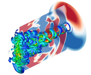
The vortical structures in the shear layer and the acoustic fields of the jets at NPRs of 2.2, 2.4 and 2.6 are provided in figure 2 and in supplementary movies (available at https://doi.org/10.1017/jfm.2020.436). For the convenience of display, a coordinate transformation has been performed from cylindrical coordinates to Cartesian coordinates by

(3.1a,b,c)\begin{equation}X/D = x,\quad Y/D = r\cos \theta ,\quad Z/D = r\sin \theta .\end{equation}

Figure 2. The instantaneous snapshots of the isosurfaces of the non-dimensional Q-criterion = 0.1, coloured by the local Mach number, and the pressure fluctuations in the planes $x = 0$, $\theta = {\rm \pi}/2$ and $3{\rm \pi} /2$ for the jets at (a) NPR = 2.2, (b) NPR = 2.4 and (c) NPR = 2.6. The nozzle exit is located at $X/D = 0$.

The jets originate from the nozzle with laminar conditions. As shown in figure 2(a) and supplementary movie 1, several axisymmetric vortex rings appear in the shear layer of the jet at the NPR of 2.2. The vortex rings gradually lose their symmetry characteristic when they move downstream. The acoustic waves propagating upstream or downstream are displayed by the fluctuating pressure fields in the planes $\theta = {\rm \pi}/2$ and $3{\rm \pi} /2$. The acoustic waves of the screech tone mainly propagate upstream and are symmetrical with respect to the jet axis. In the plane $X/D = 0$, the screech waves are shown as circles corresponding to the axisymmetric vortex rings in the shear layer.

Significant differences of vortical structures can be observed between the jets at NPRs of 2.2 and 2.4. As shown in figure 2(b) and supplementary movie 2, for the jet at the NPR of 2.4, the vortices are stronger around $\theta = {\rm \pi}/2$ and $3{\rm \pi} /2$. More complex vortices appear at downstream locations ($X/D \ge 5$) and the jet seems to transit into turbulence earlier than the jet at the NPR of 2.2. In the planes $\theta = {\rm \pi}/2$ and $3{\rm \pi} /2$, the upstream-propagating acoustic waves at the upper and lower sides of the jet have opposite phases. For the jet at the NPR of 2.6, vortices are also generated alternately on both sides of the jet, as shown in figure 2(c) and supplementary movie 3. The vortices in the shear layer as well as the acoustics field in the plane $X/D = 0$ have a more significant helical characteristic. For these three jets, the characteristics of the vortex structures and the screech waves are closely related. The modes of the screech tones will be discussed further in the following sections.

3.2. Mean fields and shock cell spacing

The spacing of the shock cell is an important length scale in locating the effective source of the screech tone. Mercier et al. (Reference Mercier, Castelain and Bailly2017) found the effective sound source is at the third or fourth shock tip over a wide range of operating conditions. The axial mean velocity fields for different jets are shown in figure 3 and the first four shock reflection points at the shear layer are marked to obtain the shock cell spacings. The axial sizes of the shock cells increase with increasing NPR. An approximate solution for the spacing of the first shock cell was given by Pack (Reference Pack1950) based on a theoretical analysis:

(3.2)\begin{equation}{\lambda _1} = 2.695\sqrt {(\textrm{NP}{\textrm{R}^{0.291}} - 1.205)} .\end{equation}

Figure 3. Axial mean velocity fields for the jets at (a) NPR = 2.2, (b) NPR = 2.4 and (c) NPR = 2.6. The black dashed lines indicate the axial positions of the shock reflection points at the jet shear layer.

Here the spacing of the first shock cell ${\lambda _1}$ is non-dimensionalized by the nozzle exit diameter D. In table 2, the spacing of the first shock cell obtained from the present numerical simulations and (3.2) are compared. Good agreement is found between the numerical and theoretical results. Moreover, the distribution of the averaged density along the centreline of the jet at the NPR of 2.4 is compared with the experimental results of Panda & Seasholtz (Reference Panda and Seasholtz1999) in figure 4. The numerical results and the experimental results also show a good agreement. These results indicate that accurate spacings of shock cells can be obtained from the present simulations.

Figure 4. Comparison of non-dimensional averaged density along the jet centreline obtained from the numerical simulation and the experiment of Panda & Seasholtz (Reference Panda and Seasholtz1999) at the NPR of 2.4.

Table 2. Comparison of non-dimensional spacings of the first shock cell obtained from the numerical simulations and from equation (3.2).

3.3. Pressure spectra and tone frequencies

Fast Fourier transforms are applied on the pressure fluctuations at every point along the circular line of $(x,r) = (0,2)$ to obtain the frequencies and the azimuthal characteristics of the screech tones. As shown in figure 5(a), the amplitude of the screech tone at $S{t_j} = 0.5804$ (the magenta arrow) distributes uniformly along the circular line $(x,r) = (0,2)$. In figure 5(b), at different azimuthal angles, the phases of the screech tone are almost the same. These results indicate that the screech tone is at an axisymmetric mode for the jet at the NPR of 2.2. In figure 5(c), at the NPR of 2.4, the screech tone at $S{t_j} = 0.4237$ (the magenta arrow) has higher amplitudes around the azimuthal angles of $\theta = {\rm \pi}/2$ and $3{\rm \pi} /2$, and becomes weak near $\theta = 0$ and ${\rm \pi} $. As shown in figure 5(d), the phase of this screech tone abruptly changes around $\theta = 0$ and ${\rm \pi} $ resulting in a phase difference of ${\rm \pi} $. Thus, this screech tone is at a flapping mode. In figure 5(c), there is another tone at $S{t_j} = 0.5778$ (the blue arrow) which has almost equivalent amplitudes from $\theta = 0$ to $2{\rm \pi} $. As shown in figure 5(d), the phase of this tone continuously fluctuates along the circular line and the phase differences between different azimuthal angles are obviously less than ${\rm \pi} $. The extreme value points on the phase curve are near$\; \theta = 0$ and ${\rm \pi} $ where the phase of the screech tone at $S{t_j} = 0.4237$ jumps. It can be inferred that the screech tone at $S{t_j} = 0.5778$ is at an axisymmetric mode, but becomes a little tilted under the influence of the flapping mode. For the jet at the NPR of 2.6, in figure 5(e), there is a screech tone at $S{t_j} = 0.3743$ (the magenta arrow) that has variable amplitudes along the circular line of $(x,r) = (0,2)$. And as shown in figure 5(f), the phase of this tone also abruptly changes leading to a phase difference of ${\rm \pi} $. Thus, this screech tone is also at a flapping mode.

Figure 5. Noise spectra (a,c,e) and phase distributions (b,d,\,f) of screech tones along the circular line $(x,r) = (0,2)$ for the jet at NPR = 2.2 (a,b), NPR = 2.4 (c,d) and NPR = 2.6 (e,f). The colours of the arrows in (a,c,e) correspond to the colours of the curves in (b,d,f).

The acoustic wavelengths of the screech tones are calculated based on the screech frequencies and the ambient sound velocity. Figure 6 shows the comparisons of the acoustic wavelengths obtained from the present numerical simulations and the experiments of Ponton & Seiner (Reference Ponton and Seiner1992). The acoustic wavelengths shown in figure 6 are non-dimensionalized by the nozzle exit diameter D. The steady increase of the acoustic wavelength with the increasing ideally expanded Mach number ${M_j}$ is segmented into several stages corresponding to the different instability modes of the jets. As shown in figure 6, at the NPR of 2.2 (${M_j} = 1.1240$), the acoustic wavelength of the screech tone falls on the extension of the curve for the A1 mode. For the jet at the NPR of 2.4 (${M_j} = 1.1921$), the acoustic wavelengths of screech tones are located at the curves for the A2 and B mode, respectively. And at the NPR of 2.6 (${M_j} = 1.2528$), the acoustic wavelength also has a good agreement with the experimental results at the B mode. Powell et al. (Reference Powell, Umeda and Ishii1992) demonstrated that the A1 and A2 modes are two toroidal modes and the B mode is a flapping mode. The characteristics of these modes agree well with the features of the screech tones that are shown in figure 5. Hu & McLaughlin (Reference Hu and McLaughlin1990) suggested that the fine-scale turbulence is extraneous to the basic screech phenomenon. In their experiments, the screech frequencies of low-Reynolds-number jets agree well with their high-Reynolds-number counterparts. The present numerical simulations are conducted on jets with a low Reynolds number and the numerical results are also in good agreement with the experimental data. On the other hand, the good agreement between numerical and experimental results also demonstrates the accuracy of the present simulations. The modes and frequencies of the screech tones in the present simulations are summarized in table 3.

Figure 6. The comparisons of screech tone acoustic wavelengths between the experiments of Ponton & Seiner (Reference Ponton and Seiner1992) (red, ▾ = A1, ∘ = A2 and ▴ = B modes for the nozzle with the lip of 0.2D; blue, ▾ = A1, ∘ = A2 and ▴ = B modes for the nozzle with the lip of 0.4D); and the present numerical simulations (black, ▾ = A1, ∘ = A2 and ▴ = B modes). ${M_j}$ is the ideally expanded Mach number.

Table 3. The modes and Strouhal numbers of the screech tones; ${M_j}$ is the ideally expanded Mach number.

At the NPR of 2.4, two screech tones are presented in figure 5(c). However, Fourier analysis cannot reveal whether these two modes are coexisting or switching in a mutually exclusive fashion. Here we investigate the dynamic characteristics of screech tones via the continuous wavelet transform (CWT) (Mancinelli et al. Reference Mancinelli, Pagliaroli, Di Marco, Camussi and Castelain2017, Reference Mancinelli, Jaunet, Jordan and Towne2019). The wavelet transform is performed on the fluctuating pressure signal. The detailed process of the CWT is given by Mancinelli et al. (Reference Mancinelli, Pagliaroli, Di Marco, Camussi and Castelain2017). The bump wavelet kernel is used here. The present CWT analyses are carried out by using the Matlab^® software.

The fluctuating pressure is obtained at 1000 instants from the numerical simulations. Because of the edge effect of the CWT, the results from the 200th to the 800th stored instants are shown. Firstly, the CWT analyses are conducted on the pressure fluctuations at a point in the nozzle exit plane for the jets at the NPRs of 2.2 and 2.6. The results are shown in figure 7(a,b), respectively. The screech frequencies and amplitudes for these two jets can remain stable in the time range of the numerical simulations. This demonstrates that the numerical simulations conducted on these two jets have reached stable states. Each screech tone corresponds to a high-amplitude band in figure 7. However, the current results are able to display the time evolutions of the screech frequencies and amplitudes.

Figure 7. Time–frequency scalograms: (a) for the NPR = 2.2 jet, at $(x,\theta ,r) = (0,{\rm \pi} /2,2)$, the blue dashed line corresponds to $S{t_j} = 0.5804$; (b) for the NPR = 2.6 jet, at $(x,\theta ,r) = (0,{\rm \pi} /2,2)$, the blue dashed line corresponds to $S{t_j} = 0.3743$ and the purple dashed line corresponds to $S{t_j} = 0.749$.

Figure 8 shows the CWT results for the jet at the NPR of 2.4. At the point $(x,\theta ,r) = (0,{\rm \pi} ,2)$, only the screech tone at the A2 mode (the purple dashed line) is detected in figure 8(a). However, at the point $(x,\theta ,r) = (0,3{\rm \pi} /2,2)$, the screech tone at the A2 mode (the purple dashed line) and the B mode (the blue dashed line) can coexist steadily in figure 8(b). Furthermore, the CWT is applied on the fluctuating pressure in the jet shear layer. As shown in figure 9, at the azimuthal angle of $3{\rm \pi} /2$, the instability waves at the B mode have a higher amplitude. The frequencies and amplitudes of the instability waves at the A2 and B modes are stable. Based on the above analyses, it can be concluded that the A2 and B modes can coexist in the jet at the NPR of 2.4. The screech tone at the B mode possessing a higher amplitude is dominant.

Figure 8. Time–frequency scalograms for the NPR = 2.4 jet: (a) at $(x,\theta ,r) = (0,{\rm \pi} ,2)$ and (b) at $(x,\theta ,r) = (0,3{\rm \pi} /2,2)$. The purple dashed line corresponds to $S{t_j} = 0.5778$, and the blue dashed line corresponds to $S{t_j} = 0.4237$.

Figure 9. Time–frequency scalogram for the NPR = 2.4 jet at $(x,\theta ,r) = (0.8,3{\rm \pi} /2,0.5)$. The purple dashed line corresponds to $S{t_j} = 0.5778$, and the blue dashed line corresponds to $S{t_j} = 0.4237$.

3.4. Fourier decomposition of the pressure field

The amplitude and phase fields of pressure fluctuations at the screech frequencies are obtained by Fourier transforms. As shown in figure 10(a–d), the amplitude fields in the $(x,r)$ planes exhibit several cell structures along the jet boundary. These structures are standing waves, which have been observed previously in supersonic screeching jets experimentally by Panda (Reference Panda1999) and numerically by Gojon & Bogey (Reference Gojon and Bogey2017). Panda (Reference Panda1999) suggested that this standing wave pattern is formed by the interference between the downstream-propagating instability waves and the upstream-propagating acoustic fluctuations. The wavenumber of the standing wave ${k_{sw}}$ can be calculated as

(3.3)\begin{equation}{k_{sw}} = {k_a} + {k_h},\end{equation}

where ${k_a}$ and ${k_h}$ are, respectively, the wavenumbers of the upstream-propagating acoustic waves and the downstream-propagating instability waves (Panda Reference Panda1999).

Figure 10. Amplitude (a–d) and phase (e–h) fields obtained in the $(x,r)$ planes for the pressure fluctuations at screech frequencies: (a,e) NPR = 2.2 and $S{t_j} = 0.5804$; (b,f) NPR = 2.4 and $S{t_j} = 0.5778$; (c,g) NPR = 2.4 and $S{t_j} = 0.4237$; (d,h) NPR = 2.6 and $S{t_j} = 0.3743$. The dashed black lines mark the axial ranges of the effective sources. The black solid lines indicate the axial positions of the shock reflection points at the jet shear layer.

Detailed information about the spatial organizations of the pressure fields at the screech frequencies is revealed by the phase fields in the $(x,r)$ planes and the nozzle exit plane. For the jet at the NPR of 2.2, the phase field at the screech frequency is symmetrical to the jet axis in figure 10(e), and is shown as an axisymmetric annular distribution in figure 11(e). Moreover, as shown in figure 11(a), the amplitudes at different azimuthal angles are nearly equivalent near the nozzle. These results further confirm that the screech tone of the jet at the NPR of 2.2 is at the axisymmetric A1 mode. Similar results are also found in figures 10(f), 11(b) and 11(f) for the screech tone at the NPR of 2.4 and $S{t_j} = 0.5778$, and confirm that this tone is at the axisymmetric A2 mode. As for the screech tone at the NPR of 2.4 and $S{t_j} = 0.4237$, the phase field appears antisymmetric with respect to the jet axis in figure 10(g) and to the line $\theta = 0$ and ${\rm \pi} $ in figure 11(g), respectively. The azimuthal directivity of this screech tone is shown in figure 11(c). The radiation pattern resembling that of an acoustic dipole is characteristic of a flapping screech mode (Shen & Tam Reference Shen and Tam2002). At the NPR of 2.6, as shown in figures 10(h), 11(d) and 11(h), the phase and amplitude fields of the screech tone at $S{t_j} = 0.3743$ also display the characteristics of a flapping screech mode. For the two screech tones at the B mode, different azimuthal directivity angles can be observed in figure 11(c,d). The azimuthal directivity angle for a screech tone at the B mode is in a random fashion.

Figure 11. Amplitude (a–d) and phase (e–h) fields obtained in the nozzle exit plane for the pressure fluctuations at screech frequencies: (a,e) NPR = 2.2 and $S{t_j} = 0.5804$; (b,f) NPR = 2.4 and $S{t_j} = 0.5778$; (c,g) NPR = 2.4 and $S{t_j} = 0.4237$; (d,h) NPR = 2.6 and $S{t_j} = 0.3743$.

To determine the effective source locations for different screech tones, the distributions of the phase along the line $r = 1.5$ in figure 10(e–h) are shown in figure 12. Except for some discontinuity points, the sign of the slope of the phase changes around a range of axial positions in different cases. The slope of the phase is inversely proportional to the phase velocity of the wave projected onto the line. The inversion of the sign of the slope implies the inversion of the propagation direction of the wave (Mercier et al. Reference Mercier, Castelain and Bailly2017). In the present study, at upstream regions, the sign of the slope is positive and the wave propagates upstream. At downstream locations, the sign of the slope is negative and the wave propagates downstream. Therefore, the effective sources of the screech tones can be determined by figure 12. The effective source locations are at $X/D = 2.5\sim3$ for the A1 mode at the NPR of 2.2, at $X/D = \textrm{3}.2\sim3.6$ for the A2 mode at the NPR of 2.4, at $X/D = 2.4\sim3$ for the B mode at the NPR of 2.4 and at $X/D = 2.7\sim3.6$ for the B mode at the NPR of 2.6. The ranges of the effective sources are marked in figure 10. The effective sources of the screech tones are located downstream of the fourth shock cell at the A1 and A2 modes and downstream of the third shock cell at the B mode.

Figure 12. The distributions of the phase along the line $r = 1.5$ in figure 10(e–h): (a) corresponds to figure 10(e), (b) corresponds to figure 10(f), (c) corresponds to figure 10(g), and (d) corresponds to figure 10(h).

For supersonic impinging jets, the acoustic feedback loop is established between the nozzle exit and the impinging plate. By considering the two semi-cells near the nozzle and the plate as one cell, the structures of hydrodynamic–acoustic standing waves contain a whole number of cells ${N_{sw}}$ (Bogey & Gojon Reference Bogey and Gojon2017). Gojon, Bogey & Marsden (Reference Gojon, Bogey and Marsden2016) demonstrated that ${N_{sw}}$ is also the number of periods ${N_p}$ contained in the feedback loop. Here, for supersonic free jets, we consider that there are two semi-cells near the nozzle and the effective source location. The number of standing wave cells, namely the number of periods contained in the screech feedback loop, can be determined from figure 10(a–d). For the A1 mode, four periods are contained in the feedback loop, the A2 mode contains five periods and there are three periods in the feedback loop at the B mode. These results are in good agreement with the experimental results of Mercier et al. (Reference Mercier, Castelain and Bailly2017). The characteristics of the screech feedback loops are summarized in table 4.

Table 4. The characteristics of the screech feedback loops: ${N_p}$ is the number of periods contained in the feedback loop; ${N_{shock}}$ is the number of shock cells between the nozzle and the effective source.

3.5. Velocity spectra

Figure 13 shows the power spectral densities (PSD) of the axial velocity fluctuations on the lip line ($r = 0.5$) at three axial positions. These spectra are azimuthally averaged. The first location of $X/D = 3$ is near or in the regions of the effective sources of the screech tones, and several peaks corresponding to the screech tones and their second harmonics can be observed. As shown in figure 13(a), for the jet at the NPR of 2.2, the peaks at $S{t_j} = 0.5804$ (the magenta arrow) and 1.18 (the green arrow) are associated with the screech tone at the A1 mode and its second harmonic, respectively. And a plateau centred around $S{t_j} = 0.29$ (the blue arrow), which is related to the subharmonic of the screech tone, also appears. For the jet at the NPR of 2.4, the peaks at $S{t_j} = 0.4237$ (the magenta arrow) and 0.5778 (the blue arrow), which are respectively associated with the screech tones at the B and A2 modes and the peak at $S{t_j} = 0.86$ (the green arrow) corresponding to the second harmonic at the B mode, are observed in figure 13(b). Because of the coexistence of these two screech modes, two humps around $S{t_j} = 0.15$ (the frequency difference between the screech tones at the A2 and B modes, the cyan arrow) and $S{t_j} = 0.28$ (the frequency difference between the screech tone at the A2 mode and the second harmonic at the B mode, the red arrow) also appear in figure 13(b). And at the NPR of 2.6, the peaks corresponding to the screech tone ($S{t_j} = 0.3743$, the magenta arrow) and the second harmonic ($S{t_j} = 0.749$, the blue arrow) can be observed in figure 13(c).

Figure 13. The power spectral densities (PSD) of non-dimensional axial velocity fluctuations ${u^{\prime}_x}$ at X/D = 3, 7 and 12 as a function of $S{t_j}$: (a) NPR = 2.2, (b) NPR = 2.4 and (c) NPR = 2.6.

At the second axial position of $X/D = 7$, the velocity spectra are shown as broadband curves. The plateau around $S{t_j} = 0.29$ is still visible for the jet at the NPR of 2.2 in figure 13(a). As shown in figure 13(b,c), because of the laminar-to-turbulent transition, a range of the spectra follows the −5/3 slope for the jets at the NPRs of 2.4 and 2.6. These results correspond to the more complex vortical structures at this axial position in figure 2(b,c). The screech tone is produced by the growth of the natural jet instability, and the jet mixing can be enhanced by the feedback loop (Raman Reference Raman1998). The enhancement of mixing depends on the mode and amplitude of the screech tone (Glass Reference Glass1968; Raman Reference Raman1998). In the present numerical simulations, for the jets at the NPRs of 2.4 and 2.6, the dominated screech tones are at the B mode and with higher amplitudes than the tones at the A1 and A2 modes. Therefore, the jets at the NPRs of 2.4 and 2.6 transit into turbulence earlier than the jet at the NPR of 2.2.

At a further downstream location of $X/D = 12$, we can observe that a range follows the −5/3 slope and a range follows the −7 slope in the spectra for all of the jets. This result agrees with the theoretical analyses of Batchelor (Reference Batchelor1953) and Heisenberg (Reference Heisenberg1985), and demonstrates that, at this location, the flow has already transited into turbulence and, in the present numerical simulations, the inertial subregion and the viscous subrange of the turbulence have been resolved.

3.6. Convection velocity

The convection velocity of the instability waves in the shear layer is an important parameter of the screech feedback loop. The screech frequencies at different modes have already been obtained. The averaged convection velocity is determined as

(3.4)\begin{equation}\overline {{U_c}} = \frac{{{\omega _s}}}{{{k_h}}},\end{equation}

where ${\omega _s}$ is the angular frequency of the screech tone. In § 3.4, Fourier transforms have been conducted on pressure fluctuations and the Fourier coefficients at the screech frequencies are obtained. The wavenumbers ${k_h}$ are determined by one-dimensional spatial Fourier transforms that are performed on the Fourier coefficients at the screech frequencies. The spatial Fourier transforms are conducted along the axial line of $r = 0.6$ and in the region of $0 \le x \le 4$ that covers the effective sources. The results are shown in figure 14. The maximum peaks are marked by the blue dashed lines in figure 14 and the corresponding wavenumbers are collected in table 5 as ${k_h}{D_j}$. The averaged convective velocity is calculated by (3.4). The convective Mach numbers ${M_c} = \overline {{U_c}} /{a_\infty }$ are shown in table 5 and range from 0.55 to 0.65. The wavenumbers corresponding to the upstream-propagating acoustic waves ${k^ - } ={-} {\omega _s}/{a_\infty }$ are represented by red dashed lines in figure 14. In each wavenumber spectrum, the central wavenumber of the highest bump in the negative wavenumber range has a good agreement with ${k^ - }$. It indicates that this bump is related to the upstream-propagating acoustic wave.

Figure 14. Normalized wavenumber spectra at screech frequencies: (a) NPR = 2.2 and $S{t_j} = 0.5804$, (b) NPR = 2.4 and $S{t_j} = 0.5778$, (c) NPR = 2.4 and $S{t_j} = 0.4237$, and (d) NPR = 2.6 and $S{t_j} = 0.3743$. The wavenumbers of ${k^ - } ={-} {\omega _s}/{a_\infty }$ are indicated by the vertical red dashed lines. The peaks in positive wavenumber range are indicated by the vertical blue dashed lines.

Table 5. The wavenumber and convective Mach number of the instability waves.

4.1. Classical feedback model

The screech tone of underexpanded free jets is due to an acoustic feedback loop, which was described in Powell (Reference Powell1953) and Tam (Reference Tam1995). This feedback mechanism establishes between the nozzle lip and the effective source. The instability waves in the jet shear layer interact with shocks around the effective source and the upstream-propagating feedback acoustic waves are produced. The feedback acoustic waves propagate to the nozzle exit outside the jet, excite the shear layer and close the feedback loop. Based on this classical feedback model, the non-dimensional screech frequency ${f_s}$ can be predicted as (Powell Reference Powell1953)

(4.1)\begin{equation}{f_s} = \frac{{{M_c}}}{{{\lambda _{sh}}(1 + {M_c})}},\end{equation}

where ${\lambda _{sh}}$ is the spacing of the shock cell non-dimensionalized by the nozzle exit diameter D. To account for the staging behaviour of the screech tone, Gao & Li (Reference Gao and Li2010) characterized each mode by the parameters ${N_p}$ and ${N_{shock}}$, and proposed a modification of (4.1):

(4.2)\begin{equation}{f_s} = \frac{{{N_p}{M_c}}}{{{N_{shock}}{\lambda _{sh}}(1 + {M_c})}}.\end{equation}

Screech frequencies are estimated by (4.2) based on the parameters given in tables 4 and 5. The spacing of the first shock cell ${\lambda _1}$ determined numerically in table 2 is used to approximate the spacing of the shock cell in (4.2). In table 6, these estimated screech frequencies are compared with the screech frequencies that are obtained from the numerical simulations. The screech frequencies estimated by the classical feedback model are in good agreement with the numerical results. However, the coexistence of the screech tones at the A2 and B modes cannot be explained by the feedback model reported above. For that reason, an alternative feedback model, which is associated with the upstream-propagating acoustic wave mode of the jet (Tam & Ahuja Reference Tam and Ahuja1990), is considered in the following section.

Table 6. Comparison of screech frequencies obtained from the numerical simulations and estimated by equation (4.2).

4.2. Combination of the feedback model and the upstream-propagating acoustic modes of the jets

The upstream-propagating neutral acoustic wave modes of high-speed jets were first identified by Tam & Hu (Reference Tam and Hu1989). In the feedback models proposed by Tam & Ahuja (Reference Tam and Ahuja1990) and Tam & Norum (Reference Tam and Norum1992), the feedback loops in subsonic round impinging jets and supersonic rectangular impinging jets are closed by the waves belonging to the upstream-propagating acoustic modes of the jets. Recently, these acoustic modes have been detected in the potential core of subsonic free jets by Towne et al. (Reference Towne, Cavalieri, Jordan, Colonius, Schmidt, Jaunet and Brès2017) and in supersonic impinging jets by Gojon et al. (Reference Gojon, Bogey and Marsden2016) and Bogey & Gojon (Reference Bogey and Gojon2017). Some evidence also demonstrates that the screech feedback loops in supersonic free jets are closed by the neutral acoustic wave modes (Edgington-Mitchell et al. Reference Edgington-Mitchell, Jaunet, Jordan, Towne, Soria and Honnery2018; Gojon et al. Reference Gojon, Bogey and Mihaescu2018; Mancinelli et al. Reference Mancinelli, Jaunet, Jordan and Towne2019).

The dispersion relation of the upstream-propagating neutral acoustic wave mode in a round jet was derived by Tam & Ahuja (Reference Tam and Ahuja1990). For the neutral acoustic wave modes considered here, both the axial wavenumber k and angular frequency $\omega $ are real numbers. The dispersion relation can be written as

(4.3)\begin{align} &|{\xi _ + }|{J_n}(|{\xi _ - }\alpha |)\dfrac{{{K_{n - 1}}(|{\xi _ + }\alpha |) + {K_{n + 1}}(|{\xi _ + }\alpha |)}}{{{K_n}(|{\xi _ + }\alpha |)}}\nonumber\\ &\quad + \dfrac{{{C^2}|{\xi _ - }|}}{{{{({a_\infty }C/{a_j} - {M_j})}^2}}}[{J_{n - 1}}(|{\xi _ - }\alpha |) - {J_{n + 1}}(|{\xi _ - }\alpha |)] = 0, \end{align}

where ${a_\infty }$ and ${a_j}$ are the sound speeds in the ambient and at the ideally expanded condition of the jet, $C = \omega /(k{a_\infty })$, ${J_n}$ is the nth-order Bessel function of the first kind, ${\xi _ + } = \,|{C^2} - 1{|^{1/2}}$, ${\xi _ - } = \,|{({a_\infty }C/{a_j} - {M_j})^2} - 1{|^{1/2}}$, $\alpha = k{D_j}/2$ and ${K_n}$ is the nth-order modified Bessel function. For the underexpanded jets in the present numerical simulations, the equivalent ideally expanded Mach number ${M_j}$ and nozzle diameter ${D_j}$ at different NPRs are given by

(4.4a,b)\begin{equation}{M_j} = \sqrt {\textrm{(NP}{\textrm{R}^{(\gamma - 1)/\gamma }} - 1)\frac{2}{{\gamma - 1}}} ,\quad \frac{{{D_j}}}{D} = {\left[ {\frac{{1 + \frac{1}{2}(\gamma - 1)M_j^2}}{{1 + \frac{1}{2}(\gamma - 1)M_e^2}}} \right]^{(\gamma + 1)/4(\gamma - 1)}}{\left( {\frac{{{M_e}}}{{{M_j}}}} \right)^{1/2}},\end{equation}

where $\gamma = 1.4$ and the exit Mach number ${M_e} = \textrm{1}$ for the convergent nozzle.

In order to combine the classical feedback model and the upstream-propagating acoustic wave mode of the jet, the wavenumber ${k_a}$ of the upstream-propagating acoustic wave in the classical feedback loop is assumed to be equal to the opposite of the wavenumber k of the upstream-propagating acoustic wave mode (Gojon et al. Reference Gojon, Bogey and Marsden2016; Bogey & Gojon Reference Bogey and Gojon2017). By considering that ${k_{sw}} = 2{\rm \pi} {N_{sw}}/({{N_{shock}}{\lambda_{sh}}} )$, ${N_{sw}} = {N_p}$, ${k_h} = 2{\rm \pi} {f_s}/{M_c}\; $ and ${k_a} ={-} k$, equation (3.3) yields

(4.5)\begin{equation}{f_s} = \frac{{{N_p}{M_c}}}{{{N_{shock}}{\lambda _{sh}}}} + \frac{{k{M_c}}}{{2{\rm \pi} }}.\end{equation}

The solutions of this equation are dependent on the location of the effective source and the averaged convection Mach number.

For each $\alpha $ and azimuthal wavenumber n, the dispersion relation (4.3) has many eigenvalues that can be ordered according to their radial wavenumber m (Tam & Hu Reference Tam and Hu1989). In what follows, the acoustic mode that corresponds to the azimuthal wavenumber n and the radial wavenumber m will be denoted by $(n,m)$ for convenience.

In figure 15, the dispersion relations of the axisymmetric acoustic wave modes for the ideally expanded jet at ${M_j} = 1.1240$ and the solutions of the feedback model (4.5) for the A1 mode at the NPR of 2.2 are shown as functions of the Strouhal number and the axial wavenumber. The screech tone at $S{t_j} = 0.5804$ is also indicated on the line $k\; ={-} \omega /{a_\infty }$. As shown in figure 15, the screech tone is located at the intersection of the line $k\; ={-} \omega /{a_\infty }$ and the line of equation (4.5) at ${N_p} = 4$, and just below the curve of the $(0,2)$ mode. The small discrepancy may be due to the presence of shocks in the simulated jet (Gojon et al. Reference Gojon, Bogey and Mihaescu2018) and the hypothesis of an inviscid infinitely thin shear layer in the vortex sheet model (Tam & Ahuja Reference Tam and Ahuja1990). In the same way, the results of the axisymmetric acoustic wave modes for the ideally expanded jet at ${M_j} = 1.1921$ and the feedback model (4.5) for the A2 mode at the NPR of 2.4 are shown in figure 16. The screech tone at $S{t_j} = 0.5778$ is very close to the intersection of the curve of the $(0,2)$ mode and the line of the feedback model (4.5) with ${N_p} = 5$. The above results are in agreement with the properties of the screech feedback loop summarized in table 4 and indicate that the screech tones at the A1 and A2 modes are generated by the feedback loops that are closed by the upstream-propagating $(0,2)$ mode of the equivalent ideally expanded jets. This conclusion agrees with the results of Edgington-Mitchell et al. (Reference Edgington-Mitchell, Jaunet, Jordan, Towne, Soria and Honnery2018).

Figure 15. Representation of the dispersion relations of the axisymmetric neutral acoustic wave modes for an ideally expanded jet at ${M_j} = 1.1240$. The red dot indicates the lower limits of the modes; the magenta dotted lines show the relation (4.5) for the A1 mode at the NPR of 2.2; and the diamond marks the screech frequency at the A1 mode.

Figure 16. Representation of the dispersion relations of the axisymmetric neutral acoustic wave modes for an ideally expanded jet at ${M_j} = 1.1921$. The red dot indicates the lower limits of the modes; the magenta dotted lines show the relation (4.5) for the A2 mode at the NPR of 2.4; and the diamond marks the screech frequency at the A2 mode.

The screech frequencies at the A1 and A2 modes are located just above or below the lower limit of the $(0,2)$ mode. As shown by the dispersion curves in figures 15 and 16, the group velocities and phase velocities of the waves near the lower limit of the $(0,2)$ mode are very close to $- {a_\infty }$. It indicates that the upstream-propagating waves that close the feedback loop should propagate at a speed that is nearly equal to $- {a_\infty }$. This is also one requirement of the classical feedback model (4.2).

The flapping B mode can be modelled by two oppositely rotating helical modes that have the same amplitude (Powell et al. Reference Powell, Umeda and Ishii1992; Ponton & Seiner Reference Ponton and Seiner1995). Thus, the relation between the screech frequencies at the B mode and the helical ($n = 1$) upstream-propagating acoustic wave modes are examined here. The results of the model combination for the jet at the NPR of 2.4 and the screech tone at the B mode are shown in figure 17. The screech tone at $S{t_j} = 0.4237$ is located at the intersection of the line $k\; ={-} \omega /{a_\infty }$ and the line of equation (4.5) at ${N_p} = 3$, and below the curve of the $(1,1)$ mode. A similar result is shown in figure 18 for the jet at the NPR of 2.6 with a larger difference between the screech frequency and the lower limit of the $(1,1)$ mode. Thus, the modified feedback model combined with the helical acoustic mode fails to estimate the screech frequency at the B mode. The screech feedback loop is closed by the upstream-propagating free-stream acoustic waves at the B mode.

Figure 17. Representation of the dispersion relations of the helical neutral acoustic wave modes for an ideally expanded jet at ${M_j}\textrm{ = 1}\textrm{.1921}$. The red dot indicates the lower limits of the modes; the magenta dotted lines show the relation (4.5) for the B mode at the NPR of 2.4; and the square marks the screech frequency at the B mode.

Figure 18. Representation of the dispersion relations of the helical neutral acoustic wave modes for an ideally expanded jet at ${M_j} = 1.2528$. The red dot indicates the lower limits of the modes; the magenta dotted lines show the relation (4.5) for the B mode at the NPR of 2.6; and the square marks the screech frequency at the B mode.

Based on the wavelet analysis in § 3.3, for the jet at the NPR of 2.4, the screech tones at the A2 and B modes can coexist. In the research of Mancinelli et al. (Reference Mancinelli, Jaunet, Jordan and Towne2019), the screech tones at the A1 and A2 modes for the underexpanded jet at ${M_j} = 1.125$ are mutually exclusive. The dispersion relations of the axisymmetric acoustic wave modes of the ideally expanded jet at ${M_j} = 1.125$ are shown in figure 19. The screech tones at $S{t_j} = 0.63$ (A1 mode) and $S{t_j} = 0.7$ (A2 mode) are obtained from Mancinelli et al. (Reference Mancinelli, Jaunet, Jordan and Towne2019) and labelled on the line $k\; ={-} \omega /{a_0}$. Both of the screech tones are located at the curve of the acoustic wave mode $(0,2)$. For the screech tones at the A1 and A2 modes, the $(0,2)$ mode is the upstream-propagating component of the feedback cycle. For the B mode, the feedback process is closed by the upstream-propagating free-stream acoustic waves. Different upstream-propagating components of the feedback loops result in the coexistence of the A2 and B modes. And the same upstream-propagating component of the feedback loop leads to the mutual exclusion between the screech tones at the A1 and A2 modes.

Figure 19. Representation of the dispersion relations of the axisymmetric neutral acoustic wave modes for an ideally expanded jet at ${M_j} = 1.125$. The red dot indicates the lower limits of the acoustic wave modes; the screech frequencies at the A1 mode (blue diamond) and A2 mode (red diamond) are obtained from Mancinelli et al. (Reference Mancinelli, Jaunet, Jordan and Towne2019).

5.1. The DMD algorithm

Unsteady flows always exhibit complex flow structures, with a wide range of temporal and spatial features. Some modal analysis techniques, such as proper orthogonal decomposition (POD; Lumley Reference Lumley, Yaglom and Tatarski1967; Sirovich Reference Sirovich1987) and dynamic mode decomposition (DMD; Schmid Reference Schmid2010), are used to extract the physically important coherent structures. The temporal coefficient of a spatial POD mode generally contains a mix of frequencies (Taira et al. Reference Taira, Brunton, Dawson, Rowley, Colonius, McKeon, Schmidt, Gordeyev, Theofilis and Ukeiley2017). DMD provides a method to decompose the time-resolved data that are obtained from numerical simulations or experiments into modes, with each mode having a single temporal frequency and growth/decay rate (Taira et al. Reference Taira, Brunton, Dawson, Rowley, Colonius, McKeon, Schmidt, Gordeyev, Theofilis and Ukeiley2017). Thus, the coherent flow structures associated with the screech tones are extracted by DMD in the present paper. The key steps of DMD (Schmid Reference Schmid2010) are outlined briefly in what follows.

The instantaneous data are represented in the form of a snapshot sequence, and two data matrices are given as

(5.1a,b)\begin{equation}{\boldsymbol{\mathsf{V}}_1} = \{ {\boldsymbol{v}_0},{\boldsymbol{v}_1},{\boldsymbol{v}_2}, \ldots ,{\boldsymbol{v}_{N - 1}}\} ,\quad \; {\boldsymbol{\mathsf{V}}_2} = \{ {\boldsymbol{v}_1},{\boldsymbol{v}_2},{\boldsymbol{v}_3}, \ldots ,{\boldsymbol{v}_N}\} ,\end{equation}

where ${\boldsymbol{v}_i}$ is the data sample at the ith temporal instant. We assume that a linear mapping $\boldsymbol{\mathsf{A}}$ connects these two matrices, that is

(5.2)\begin{equation}{\boldsymbol{\mathsf{V}}_2} = \boldsymbol{\mathsf{A}}{\boldsymbol{\mathsf{V}}_1}.\end{equation}

A singular value decomposition on the data matrix ${\boldsymbol{\mathsf{V}}_1}$ is performed,

(5.3)\begin{equation}{\boldsymbol{\mathsf{V}}_1} = \boldsymbol{\mathsf{U}}\boldsymbol{\varSigma }{\boldsymbol{\mathsf{W}}^\textrm{H}},\end{equation}

where the superscript ‘H’ denotes conjugate transpose. By combining the result of the singular value decomposition and (5.2), we obtain that

(5.4)\begin{equation}{\boldsymbol{\mathsf{U}}^\textrm{H}}\boldsymbol{\mathsf{AU}} = {\boldsymbol{\mathsf{U}}^\textrm{H}}{\boldsymbol{\mathsf{V}}_2}\boldsymbol{\mathsf{W}}{\boldsymbol{\varSigma }^{ - 1}} \equiv \tilde{\boldsymbol{\mathsf{S}}}.\end{equation}

The DMD eigenvalues ${\mu _i}$ are obtained by solving the following eigenvalue problem:

(5.5)\begin{equation}\tilde{\boldsymbol{\mathsf{S}}}{\boldsymbol{y}_i} = {\mu _i}{\boldsymbol{y}_i}.\end{equation}

And the DMD modes ${\boldsymbol{\varPhi }_i}$ are obtained by

(5.6)\begin{equation}{\boldsymbol{\varPhi }_i} = \boldsymbol{\mathsf{U}}{\boldsymbol{y}_i}.\end{equation}

5.2. DMD results

In the present DMD, the instantaneous flow variables of the non-dimensional velocity components ${u_x}$, ${u_\theta }$, ${u_r}$ and pressure p are analysed simultaneously. The data from two-dimensional sections of the flow field constitute the data sample at each instant. The total number of snapshots is 501 and the non-dimensional time interval is 0.05.

At different NPRs, the screech frequencies are obtained by the Fourier transforms conducted on the fluctuating pressure in § 3.3. Thus, the DMD modes whose frequencies are nearest to the screech frequencies are chosen and analysed in detail. For different screech tones, the data in different azimuthal planes are processed by the DMD algorithm. The subdomain considered in the current DMD analyses extends from $x ={-} 2$ to $x = 5$, which covers the effective source location at each screech mode. The frequencies of the chosen DMD modes are compared with the screech frequencies in table 7.

Table 7. Strouhal numbers of the chosen DMD modes.

The DMD mode at $S{t_j} = 0.5882$ for the jet at the NPR of 2.2 is shown in figure 20. The contour levels of the pressure component are adjusted to show the acoustic waves in the ambient of the jet. In figure 20(a), the upstream-propagating acoustic waves around the jet are observed and these waves are symmetric with respect to the jet axis. The symmetrical distributions of the axial and radial velocity components correspond to the axisymmetric vortices that are shown in figure 2(a). Moreover, there is nearly nothing shown in the azimuthal velocity component. These results indicate that the flow structures associated with the A1 mode are axisymmetric and have no observable azimuthal motions.

Figure 20. The real part of the DMD mode at $S{t_j} = 0.5882$ for the NPR = 2.2 jet in the planes $\theta \; = \; 0$ and ${\rm \pi} $: (a) the pressure component ${\varPhi _p}$, (b) the axial velocity component ${\varPhi _{{u_x}}}$, (c) the azimuthal velocity component ${\varPhi _{{u_\theta }}}$ and (d) the radial velocity component ${\varPhi _{{u_r}}}$.

For the jet at the NPR of 2.4, the dominant screech tone is at the B mode. The DMD mode at $S{t_j} = 0.4317$ is shown in figure 21. In figure 21(a), the upstream-propagating acoustic waves are out of phase relative to the jet axis. The antisymmetric patterns of the axial and radial velocity components in the jet shear layer correspond to the antisymmetric vortices that are shown in figure 2(b). And the flapping motions of the jet in the planes $\theta = {\rm \pi}/2$ and $3{\rm \pi} /2$ are also represented by the antisymmetric distribution of the radial velocity around the jet axis. As shown in figure 21(c), upstream of the effective source, there is nearly nothing displayed by the azimuthal velocity component. Because of the enhancement of the jet mixing, scattered distributions of the azimuthal velocity can be observed downstream of the effective source.

Figure 21. The real part of the DMD mode at $S{t_j} = 0.4317$ for the NPR = 2.4 jet in the planes $\theta \; = \; {\rm \pi}/2$ and $3{\rm \pi} /2$: (a) the pressure component ${\varPhi _p}$, (b) the axial velocity component ${\varPhi _{{u_x}}}$, (c) the azimuthal velocity component ${\varPhi _{{u_\theta }}}$ and (d) the radial velocity component ${\varPhi _{{u_r}}}$.

At the NPR of 2.4, the A2 and B modes are coexisting. The DMD mode at $S{t_j} = 0.5789$ in the planes $\theta = 0$ and ${\rm \pi} $ is shown in figure 22. The symmetrical distributions of the pressure, axial velocity and radial velocity are observed in figure 22(a,b,d). These results represent the axisymmetric characteristics of the A2 mode. However, as shown in figure 22(c), the distribution of azimuthal velocity is nearly antisymmetric. The antisymmetric distribution of the azimuthal velocity is a representation of the motion that is vertical to the plane. By considering that the coherent structures associated with the B mode show a flapping motion in the planes $\theta \; = \; {\rm \pi}/2$ and $3{\rm \pi} /2$, which are vertical to the planes in figure 22, it can be concluded that the flow structures associated with the A2 mode display a slight oscillation that is vertical to the planes $\theta \; = \; 0$ and ${\rm \pi} $ under the influence of the flow structures associated with the B mode.

Figure 22. The real part of the DMD mode at $S{t_j} = 0.5789$ for the NPR = 2.4 jet in the planes $\theta \; = \; 0$ and ${\rm \pi} $: (a) the pressure component ${\varPhi _p}$, (b) the axial velocity component ${\varPhi _{{u_x}}}$, (c) the azimuthal velocity component ${\varPhi _{{u_\theta }}}$ and (d) the radial velocity component ${\varPhi _{{u_r}}}$.

As for the B mode of the jet at the NPR of 2.6, the DMD mode at $S{t_j} = 0.3806$ in the planes $\theta \; = \; 0$ and ${\rm \pi} $ is shown in figure 23. As shown in figure 23(a,b,d), the distributions of the pressure, axial velocity and radial velocity are antisymmetric corresponding to the characteristics of the flapping B mode. As shown in figure 23(d), the in-plane flapping motions of the jet and the shock that is located at $x = 1.5 \sim 2$ are displayed by the antisymmetric distribution of the radial velocity near the jet axis. Furthermore, the symmetric distribution of the azimuthal velocity is observed in figure 23(c) and this is a representation of the rotational movement in the azimuthal direction.

Figure 23. The real part of the DMD mode at $S{t_j} = 0.3806$ for the NPR = 2.6 jet in the planes $\theta \; = \; 0$ and ${\rm \pi} $: (a) the pressure component ${\varPhi _p}$, (b) the axial velocity component ${\varPhi _{{u_x}}}$, (c) the azimuthal velocity component ${\varPhi _{{u_\theta }}}$ and (d) the radial velocity component ${\varPhi _{{u_r}}}$.