


1 Introduction
Launder & Rodi (Reference Launder and Rodi1983) defined a wall jet as ‘a boundary layer in which, by virtue of the initially supplied momentum, the velocity over some region in the shear layer exceeds that in the free stream’. Normally, for a wall jet, fluid exits from a slot at high velocity and flows along a wall. Wall jets are characterized by the presence and interaction of two shear layers. The first is from the boundary layer, developing due to the high momentum fluid along the wall, also called the ‘inner layer’. The second develops between the high momentum fluid of the jet and the outer ambient conditions, which can be quiescent, or moving with a different speed than the jet and is called the ‘outer layer’. The two layers have different kinds of large scale structures responsible for the generation of shear strain, which produce turbulence. These structures interact with each other. The inlet wall jet Reynolds number can be defined as
 $Re_{j}=U_{j}h/\unicode[STIX]{x1D708}$
, where
$Re_{j}=U_{j}h/\unicode[STIX]{x1D708}$
, where
 $h$
is the slot height,
$h$
is the slot height,
 $U_{j}$
is the jet slot exit velocity and
$U_{j}$
is the jet slot exit velocity and
 $\unicode[STIX]{x1D708}$
is the kinematic viscosity. The mean streamwise velocity profile of a turbulent wall jet in the fully developed region is shown in figure 1. This profile is characterized by a maximum velocity
$\unicode[STIX]{x1D708}$
is the kinematic viscosity. The mean streamwise velocity profile of a turbulent wall jet in the fully developed region is shown in figure 1. This profile is characterized by a maximum velocity
 $U_{max}$
, which separates the two layers in this flow. The location of the maximum velocity is designated as
$U_{max}$
, which separates the two layers in this flow. The location of the maximum velocity is designated as
 $y_{max}$
. A length scale for the outer layer is defined as
$y_{max}$
. A length scale for the outer layer is defined as
 $y_{1/2}$
. This is the wall-normal distance above
$y_{1/2}$
. This is the wall-normal distance above
 $y_{max}$
, where the streamwise velocity is half of the maximum velocity i.e.
$y_{max}$
, where the streamwise velocity is half of the maximum velocity i.e.
 $(1/2)U_{max}$
. A similar length scale
$(1/2)U_{max}$
. A similar length scale
 $(y_{1/2})_{in}$
can be defined for the inner layer, which is the wall-normal distance below
$(y_{1/2})_{in}$
can be defined for the inner layer, which is the wall-normal distance below
 $y_{max}$
, where the streamwise velocity again becomes
$y_{max}$
, where the streamwise velocity again becomes
 $(1/2)U_{max}$
.
$(1/2)U_{max}$
.

Figure 1. Various length and velocity parameters used for wall jet scaling.
Wall jets find wide ranging application in separation control on airfoils (Dunham Reference Dunham1968), and in the film cooling of combustion chamber liners and leading stage blades in gas turbines (Launder & Rodi Reference Launder and Rodi1983). In the case of separation control, the objective is to achieve enhanced near wall momentum and increased mixing between the wall jet and the outer flow to suppress separation. On the other hand, for film-cooling applications, the jet and ambient flow should have minimum mixing. These are opposite requirements and for efficient application, a greater understanding of this flow is needed at more relevant Reynolds numbers.
Since Glauert (Reference Glauert1956), who coined the term wall jet and made the first attempt to achieve a boundary layer solution for this, several analytical, experimental and numerical studies have been performed. Launder & Rodi (Reference Launder and Rodi1983) gave a comprehensive overview of pre-1980 wall jet research. More recently Banyassady & Piomelli (Reference Banyassady and Piomelli2014) reviewed the latest work on wall jets. A significant amount of work is concerned with the self-similar solution or behaviour of the wall jet. George et al. (Reference George, Abrahamsson, Eriksson, Karlsson, Lofdahal and Wosnik2000) explained the significant benefits in defining self-similarity as follows: ‘Only a similarity solution provides an unambiguous test of a turbulence model independent of computational constraints and experimental difficulties. It does not depend on computational grid, domain, or differencing schemes, nor does it depend on difficulties in realizing and measuring a laboratory flow. It exists independent of closure approximations, and thus the scaling laws it offers can be used to test closure hypotheses. Its straightforward boundary conditions are free from the finite limits of experimental facilities or computer memories, and thus its profiles provide an ideal reference for testing the effects of enclosure’.
A similarity solution was obtained by dividing the wall jet into inner and outer layers (Glauert Reference Glauert1956; Schwarz & Cosart Reference Schwarz and Cosart1961; Myers, Schauer & Eustis Reference Myers, Schauer and Eustis1963). The inner layer is considered similar to the boundary layer, with
 $U_{max}$
as the free stream velocity and
$U_{max}$
as the free stream velocity and
 $y_{max}$
acting as the boundary layer thickness. The outer layer above
$y_{max}$
acting as the boundary layer thickness. The outer layer above
 $y_{max}$
is treated as half of a free jet. This is a remarkably simple picture, however it is not supported by measurements. The inner layer does not follow the turbulent boundary layer behaviour exactly and is influenced by the outer layer turbulence. Also, the outer layer does not expand like a free jet due to the presence of the wall.
$y_{max}$
is treated as half of a free jet. This is a remarkably simple picture, however it is not supported by measurements. The inner layer does not follow the turbulent boundary layer behaviour exactly and is influenced by the outer layer turbulence. Also, the outer layer does not expand like a free jet due to the presence of the wall.
Irwin (Reference Irwin1973) and Wygnanski, Katz & Horev (Reference Wygnanski, Katz and Horev1992) used
 $y_{1/2}$
and
$y_{1/2}$
and
 $U_{max}$
, as length and velocity scales, respectively. Irwin (Reference Irwin1973) showed that measured mean streamwise velocity, Reynolds normal and shear stresses, scale with these parameters. However, Wygnanski et al. (Reference Wygnanski, Katz and Horev1992) showed that only streamwise velocity profiles collapse with this scaling.
$U_{max}$
, as length and velocity scales, respectively. Irwin (Reference Irwin1973) showed that measured mean streamwise velocity, Reynolds normal and shear stresses, scale with these parameters. However, Wygnanski et al. (Reference Wygnanski, Katz and Horev1992) showed that only streamwise velocity profiles collapse with this scaling.
George et al. (Reference George, Abrahamsson, Eriksson, Karlsson, Lofdahal and Wosnik2000) showed that for finite Reynolds numbers wall jets cannot have a similarity solution. However, in the limit of infinite Reynolds number, mean flow and Reynolds stress profiles can collapse with appropriate scaling parameters. In the inner layer region, mean streamwise velocity and Reynolds stresses are scaled with the friction velocity
 $u_{\unicode[STIX]{x1D70F}}=\sqrt{\unicode[STIX]{x1D708}\unicode[STIX]{x2202}u/\unicode[STIX]{x2202}y|_{y=0}}$
and friction length
$u_{\unicode[STIX]{x1D70F}}=\sqrt{\unicode[STIX]{x1D708}\unicode[STIX]{x2202}u/\unicode[STIX]{x2202}y|_{y=0}}$
and friction length
 $\unicode[STIX]{x1D708}/u_{\unicode[STIX]{x1D70F}}$
, where
$\unicode[STIX]{x1D708}/u_{\unicode[STIX]{x1D70F}}$
, where
 $\unicode[STIX]{x1D708}$
is the kinematic viscosity. In the outer layer, streamwise velocity and Reynolds normal stresses are scaled with
$\unicode[STIX]{x1D708}$
is the kinematic viscosity. In the outer layer, streamwise velocity and Reynolds normal stresses are scaled with
 $U_{max}$
and
$U_{max}$
and
 $y_{1/2}$
, whereas the Reynolds shear stress is scaled with both
$y_{1/2}$
, whereas the Reynolds shear stress is scaled with both
 $U_{max}$
and
$U_{max}$
and
 $u_{\unicode[STIX]{x1D70F}}$
. More recently Barenblatt, Chorin & Prostokishin (Reference Barenblatt, Chorin and Prostokishin2005) showed that the wall jet has two self-similar layers i.e. outer and wall layers. Both of these layers show a strong influence of the inlet slot height or incomplete similarity. The velocity scale for this similarity is
$u_{\unicode[STIX]{x1D70F}}$
. More recently Barenblatt, Chorin & Prostokishin (Reference Barenblatt, Chorin and Prostokishin2005) showed that the wall jet has two self-similar layers i.e. outer and wall layers. Both of these layers show a strong influence of the inlet slot height or incomplete similarity. The velocity scale for this similarity is
 $U_{max}$
, whereas the length scales are
$U_{max}$
, whereas the length scales are
 $y_{1/2}$
and
$y_{1/2}$
and
 $(y_{1/2})_{in}$
for the outer and wall layers, respectively. This incomplete similarity is at variance with George et al. (Reference George, Abrahamsson, Eriksson, Karlsson, Lofdahal and Wosnik2000), which has only one length scale for the mean flow. Eriksson, Karlsson & Persson (Reference Eriksson, Karlsson and Persson1998) and Rostamy et al. (Reference Rostamy, Bergstrom, Sumner and Bugg2011a
) showed that the measured mean streamwise velocity and all Reynolds stresses scale with the parameters defined by George et al. (Reference George, Abrahamsson, Eriksson, Karlsson, Lofdahal and Wosnik2000). Tang et al. (Reference Tang, Rostamy, Bergstrom, Bugg and Sumner2015) showed that inner layer mean velocity profiles collapse with the similarity parameters defined by Barenblatt et al. (Reference Barenblatt, Chorin and Prostokishin2005). Efforts have also been made to identify the inner layer region with the standard log law, which is given for boundary layers as
$(y_{1/2})_{in}$
for the outer and wall layers, respectively. This incomplete similarity is at variance with George et al. (Reference George, Abrahamsson, Eriksson, Karlsson, Lofdahal and Wosnik2000), which has only one length scale for the mean flow. Eriksson, Karlsson & Persson (Reference Eriksson, Karlsson and Persson1998) and Rostamy et al. (Reference Rostamy, Bergstrom, Sumner and Bugg2011a
) showed that the measured mean streamwise velocity and all Reynolds stresses scale with the parameters defined by George et al. (Reference George, Abrahamsson, Eriksson, Karlsson, Lofdahal and Wosnik2000). Tang et al. (Reference Tang, Rostamy, Bergstrom, Bugg and Sumner2015) showed that inner layer mean velocity profiles collapse with the similarity parameters defined by Barenblatt et al. (Reference Barenblatt, Chorin and Prostokishin2005). Efforts have also been made to identify the inner layer region with the standard log law, which is given for boundary layers as
 $\langle u\rangle ^{+}=A\ln (y^{+})+B$
with
$\langle u\rangle ^{+}=A\ln (y^{+})+B$
with
 $\langle u\rangle ^{+}=\langle u\rangle /u_{\unicode[STIX]{x1D70F}}$
,
$\langle u\rangle ^{+}=\langle u\rangle /u_{\unicode[STIX]{x1D70F}}$
,
 $y^{+}=yu_{\unicode[STIX]{x1D70F}}/\unicode[STIX]{x1D708}$
,
$y^{+}=yu_{\unicode[STIX]{x1D70F}}/\unicode[STIX]{x1D708}$
,
 $A=2.44$
and
$A=2.44$
and
 $B=5.0$
. Banyassady & Piomelli (Reference Banyassady and Piomelli2015) have compiled values of
$B=5.0$
. Banyassady & Piomelli (Reference Banyassady and Piomelli2015) have compiled values of
 $A$
and
$A$
and
 $B$
for various wall jet studies and showed that there is a large scatter in the published data. George et al. (Reference George, Abrahamsson, Eriksson, Karlsson, Lofdahal and Wosnik2000) have suggested a power-law profile, which unlike the log law covers the entire inner layer.
$B$
for various wall jet studies and showed that there is a large scatter in the published data. George et al. (Reference George, Abrahamsson, Eriksson, Karlsson, Lofdahal and Wosnik2000) have suggested a power-law profile, which unlike the log law covers the entire inner layer.
Apart from self-similar behaviour, there are other aspects of wall jets which need attention from the application point of view. Applications such as flow control or heat transfer require greater understanding of inner and outer layer interaction and the development and interaction of large scale structures. In order to explain turbulence structure, turbulence kinetic energy and Reynolds stress budgets are needed both in the inner and outer layer regions. There are few studies which address any of these issues. Irwin (Reference Irwin1973) and Zhou, Heine & Wygnanski (Reference Zhou, Heine and Wygnanski1996) may be the only two examples of wall jet experimental investigations, that have provided the turbulence kinetic energy budget and Irwin (Reference Irwin1973) may be the only one for the Reynolds stress budget. Measurements can provide only a few terms pertaining to dissipation directly and most of the budget terms have to be estimated using various assumptions (Zhou et al. Reference Zhou, Heine and Wygnanski1996). Moreover, experiments have provided the budgets only in the outer layer region.
In order to investigate wall jets in greater detail, numerical techniques like large-eddy simulation (LES) and direct numerical simulation (DNS) are invaluable. Dejoan & Leschziner (Reference Dejoan and Leschziner2005) performed LES of a wall jet at a reasonably high Reynolds number of
 $Re_{j}=9700$
. However, their domain length was limited to
$Re_{j}=9700$
. However, their domain length was limited to
 $22h$
, which means they might not have achieved the fully developed self-similar state. The outer and inner layer budgets for turbulence kinetic energy and Reynolds stresses were presented. They showed that turbulent diffusion transfers turbulent kinetic energy from the inner and outer layers, where the production peaks exist, to the overlap region with minimal production. Ahlman, Brethouwer & Johansson (Reference Ahlman, Brethouwer and Johansson2007) performed the first DNS for a wall jet at a relatively low Reynolds number of
$22h$
, which means they might not have achieved the fully developed self-similar state. The outer and inner layer budgets for turbulence kinetic energy and Reynolds stresses were presented. They showed that turbulent diffusion transfers turbulent kinetic energy from the inner and outer layers, where the production peaks exist, to the overlap region with minimal production. Ahlman, Brethouwer & Johansson (Reference Ahlman, Brethouwer and Johansson2007) performed the first DNS for a wall jet at a relatively low Reynolds number of
 $Re_{j}=2000$
. Their focus was on the dynamic and mixing properties of a wall jet. They considered the scalar transport and presented the mixing properties in terms of mean scalar values, scalar flux, dissipation and various scalings for these properties. Ahlman et al. (Reference Ahlman, Velter, Brethouwer and Johansson2009) also considered low Mach number wall jets with a considerable density gradient between the jet and its surroundings. This work showed the influence of density gradient on the development of wall jets, which is important for film-cooling and combustion applications.
$Re_{j}=2000$
. Their focus was on the dynamic and mixing properties of a wall jet. They considered the scalar transport and presented the mixing properties in terms of mean scalar values, scalar flux, dissipation and various scalings for these properties. Ahlman et al. (Reference Ahlman, Velter, Brethouwer and Johansson2009) also considered low Mach number wall jets with a considerable density gradient between the jet and its surroundings. This work showed the influence of density gradient on the development of wall jets, which is important for film-cooling and combustion applications.
In a series of papers, Pouransari, Brethouwer & Johansson (Reference Pouransari, Brethouwer and Johansson2011), Pouransari, Vervisch & Johansson (Reference Pouransari, Vervisch and Johansson2013, Reference Pouransari, Vervisch and Johansson2014), Pouransari, Biferale & Johansson (Reference Pouransari, Biferale and Johansson2015) studied wall jets with chemical reaction or combustion. Most of these studies are confined to relatively low Reynolds number. However, they addressed fundamental issues involving the effect of chemical reactions and associated heat release on the mixing present in wall jet flows. Pouransari et al. (Reference Pouransari, Vervisch and Johansson2013) showed that the heat release delays transition and increases density, pressure and species concentration fluctuations. It also dampens the velocity fluctuations and Reynolds shear stress, which enlarge the finer scale structures and produce larger vortices. The effect of Reynolds number on reacting turbulent wall jets was also investigated (Pouransari et al.
Reference Pouransari, Vervisch and Johansson2014). Wall jets at Reynolds numbers
 $Re_{j}=2000$
and
$Re_{j}=2000$
and
 $Re_{j}=6000$
were compared. This work showed that the flame and turbulent structures become finer at higher Reynolds number.
$Re_{j}=6000$
were compared. This work showed that the flame and turbulent structures become finer at higher Reynolds number.
Recently Banyassady & Piomelli (Reference Banyassady and Piomelli2014) performed LES of a wall jet on smooth and rough surfaces. They considered a long domain up to
 $35h$
at a Reynolds number of
$35h$
at a Reynolds number of
 $Re=7500$
, which provided a fully developed wall jet. These computations showed that, for the roughness height and Reynolds number considered, the effects of roughness are confined to the inner layer. Hence, the turbulence structures and scaling parameters for the outer layer are not affected by the roughness. In the inner layer region, roughness redistributes wall-normal and spanwise turbulence towards isotropy. Banyassady & Piomelli (Reference Banyassady and Piomelli2015) further extended LES to even higher Reynolds numbers up to
$Re=7500$
, which provided a fully developed wall jet. These computations showed that, for the roughness height and Reynolds number considered, the effects of roughness are confined to the inner layer. Hence, the turbulence structures and scaling parameters for the outer layer are not affected by the roughness. In the inner layer region, roughness redistributes wall-normal and spanwise turbulence towards isotropy. Banyassady & Piomelli (Reference Banyassady and Piomelli2015) further extended LES to even higher Reynolds numbers up to
 $Re_{j}=40\,000$
. They compared plane and radial wall jets and showed that even though the radial wall jet has one more direction to expand, it is fundamentally similar to a plane wall jet. They also showed that the local Reynolds number determines the intrusion of the outer layer in to the inner layer. The interaction of the outer layer with the inner layer is weaker with increasing local Reynolds number.
$Re_{j}=40\,000$
. They compared plane and radial wall jets and showed that even though the radial wall jet has one more direction to expand, it is fundamentally similar to a plane wall jet. They also showed that the local Reynolds number determines the intrusion of the outer layer in to the inner layer. The interaction of the outer layer with the inner layer is weaker with increasing local Reynolds number.
In this paper a DNS of a wall jet at a Reynolds number of
 $Re_{j}=7500$
for a domain longer than
$Re_{j}=7500$
for a domain longer than
 $40h$
is reported. To the best of authors’ knowledge, this Reynolds number is the highest and the domain range the longest for any reported DNS of a wall jet. This particular Reynolds number is selected in order to compare the DNS results with the experiments of Rostamy et al. (Reference Rostamy, Bergstrom, Sumner and Bugg2011a
,Reference Rostamy, Bergstrom, Sumner and Bugg
b
), Tang et al. (Reference Tang, Rostamy, Bergstrom, Bugg and Sumner2015) and numerical simulations of Banyassady & Piomelli (Reference Banyassady and Piomelli2014, Reference Banyassady and Piomelli2015). The highly resolved unsteady flow field is used to present large scale coherent structures in the transition and fully developed regions in the inner and outer layers. Hence a clear picture of the complex unsteady flow physics is presented. The mean flow field, Reynolds normal and shear stresses are presented with the various scalings given in the literature. The turbulence kinetic energy, Reynolds normal and shear stress budgets are directly calculated and presented both in the inner and outer layers.
$40h$
is reported. To the best of authors’ knowledge, this Reynolds number is the highest and the domain range the longest for any reported DNS of a wall jet. This particular Reynolds number is selected in order to compare the DNS results with the experiments of Rostamy et al. (Reference Rostamy, Bergstrom, Sumner and Bugg2011a
,Reference Rostamy, Bergstrom, Sumner and Bugg
b
), Tang et al. (Reference Tang, Rostamy, Bergstrom, Bugg and Sumner2015) and numerical simulations of Banyassady & Piomelli (Reference Banyassady and Piomelli2014, Reference Banyassady and Piomelli2015). The highly resolved unsteady flow field is used to present large scale coherent structures in the transition and fully developed regions in the inner and outer layers. Hence a clear picture of the complex unsteady flow physics is presented. The mean flow field, Reynolds normal and shear stresses are presented with the various scalings given in the literature. The turbulence kinetic energy, Reynolds normal and shear stress budgets are directly calculated and presented both in the inner and outer layers.
2 Numerical simulation
Incompressible flow is considered for the wall jet in this study. This is governed by the conservation of mass and momentum:
 $$\begin{eqnarray}\displaystyle & \displaystyle \frac{\unicode[STIX]{x2202}u_{i}}{\unicode[STIX]{x2202}x_{i}}=0, & \displaystyle\end{eqnarray}$$
 $$\begin{eqnarray}\displaystyle & \displaystyle \frac{\unicode[STIX]{x2202}u_{i}}{\unicode[STIX]{x2202}t}+\frac{\unicode[STIX]{x2202}u_{i}u_{j}}{\unicode[STIX]{x2202}x_{j}}=-\frac{\unicode[STIX]{x2202}p}{\unicode[STIX]{x2202}x_{i}}+\frac{1}{Re_{j}}\frac{\unicode[STIX]{x2202}^{2}u_{i}}{\unicode[STIX]{x2202}x_{j}\unicode[STIX]{x2202}x_{j}}, & \displaystyle\end{eqnarray}$$
where
 $\{x_{1},x_{2},x_{3}\}=\{x,y,z\}$
are the coordinates in the streamwise, wall-normal and spanwise directions, respectively. The corresponding instantaneous velocities are given as
$\{x_{1},x_{2},x_{3}\}=\{x,y,z\}$
are the coordinates in the streamwise, wall-normal and spanwise directions, respectively. The corresponding instantaneous velocities are given as
 $\{u_{1},u_{2},u_{3}\}=\{u,v,w\}$
and the instantaneous pressure by
$\{u_{1},u_{2},u_{3}\}=\{u,v,w\}$
and the instantaneous pressure by
 $p$
.
$p$
.
A second-order finite volume solver is used to solve (2.1) and (2.2). The solver is based on a fractional step scheme. The spatial derivatives are discretized with second-order central differencing. The momentum equation is advanced in time with a semi-implicit scheme. In this procedure the convective terms are treated explicitly using the Adams–Bashforth scheme and diffusive terms are solved implicitly with the Crank–Nicolson method. The Poisson equation for pressure is transformed to Fourier space by applying fast Fourier transforms in the spanwise direction. This results in a system of equations for two-dimensional planes for each Fourier mode, which are then solved using the bi-conjugate gradient stabilized method. The solver is parallelized with message passing interface (MPI). It has been used extensively to simulate turbulent flows (Radhakrishnan et al. Reference Radhakrishnan, Keating, Piomelli and Lopes2006a ,Reference Radhakrishnan, Piomelli, Keating and Lopes b ; Naqavi, Tucker & Liu Reference Naqavi, Tucker and Liu2014).
The computational domain is in the shape of a rectangular cuboid. This has the dimensions of
 $L_{x}/h=43.0$
,
$L_{x}/h=43.0$
,
 $L_{y}/h=40.0$
and
$L_{y}/h=40.0$
and
 $L_{z}/h=9.0$
in the streamwise, wall-normal and spanwise directions, respectively. The spanwise width of the domain is comparable to several previously reported wall jet simulations (Dejoan & Leschziner Reference Dejoan and Leschziner2005; Ahlman et al.
Reference Ahlman, Velter, Brethouwer and Johansson2009; Banyassady & Piomelli Reference Banyassady and Piomelli2014; Pouransari et al.
Reference Pouransari, Vervisch and Johansson2014). The spanwise two-point correlation coefficient at
$L_{z}/h=9.0$
in the streamwise, wall-normal and spanwise directions, respectively. The spanwise width of the domain is comparable to several previously reported wall jet simulations (Dejoan & Leschziner Reference Dejoan and Leschziner2005; Ahlman et al.
Reference Ahlman, Velter, Brethouwer and Johansson2009; Banyassady & Piomelli Reference Banyassady and Piomelli2014; Pouransari et al.
Reference Pouransari, Vervisch and Johansson2014). The spanwise two-point correlation coefficient at
 $x/h=30$
for all the velocity components goes to zero by
$x/h=30$
for all the velocity components goes to zero by
 $z/h=2$
. The wall jet requires a careful selection of inflow, outflow and entrainment conditions for an efficient and accurate computation. The absence of proper conditions may result in a large recirculation in the latter part of the domain and reduces the effective streamwise range of the simulation (Levin, Herbst & Henningson Reference Levin, Herbst and Henningson2006).
$z/h=2$
. The wall jet requires a careful selection of inflow, outflow and entrainment conditions for an efficient and accurate computation. The absence of proper conditions may result in a large recirculation in the latter part of the domain and reduces the effective streamwise range of the simulation (Levin, Herbst & Henningson Reference Levin, Herbst and Henningson2006).
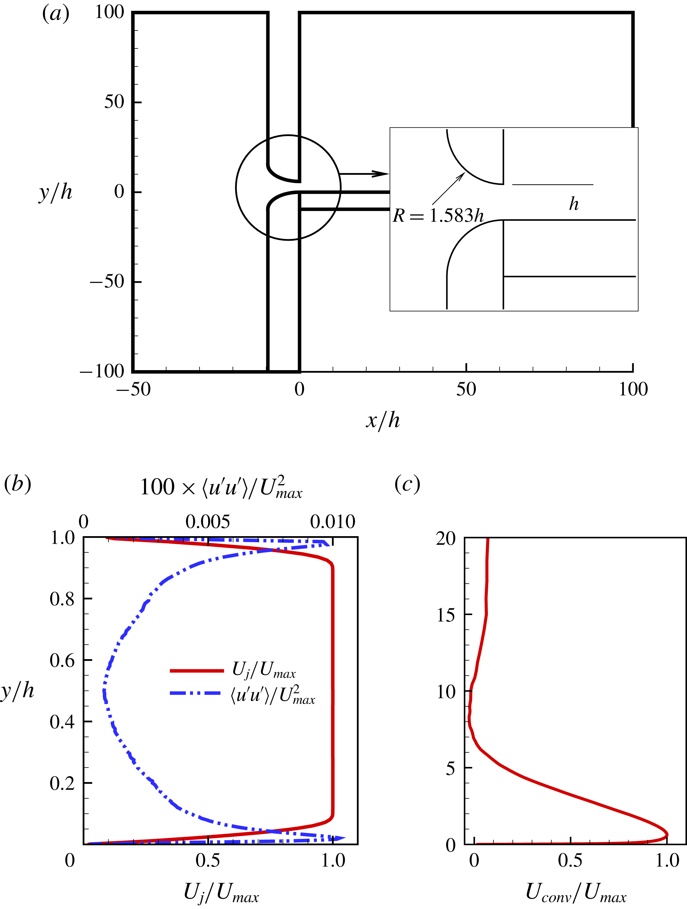
Figure 2. (a) Inlet nozzle geometry from the experiment (Rostamy et al.
Reference Rostamy, Bergstrom, Sumner and Bugg2011b
), (b) mean streamwise velocity and Reynolds stress at the inlet slot
 $(x/h=0)$
and (c) mean convective velocity
$(x/h=0)$
and (c) mean convective velocity
 $U_{conv}$
profile for the outflow boundary condition.
$U_{conv}$
profile for the outflow boundary condition.
The inlet flow conditions at the jet slot determine the transition of the jet shear layer and the wall boundary layer in numerical simulations. Previously, Ahlman et al. (Reference Ahlman, Brethouwer and Johansson2007) used a tangent hyperbolic profile for the streamwise velocity with prescribed fluctuations at the jet slot inlet. To avoid any large recirculation in the domain, they prescribed a co-flow of 10 % of the jet inlet velocity for the rest of the inlet plane. Dejoan & Leschziner (Reference Dejoan and Leschziner2005) used an experimentally measured (Eriksson et al.
Reference Eriksson, Karlsson and Persson1998) laminar profile superimposed with random fluctuations. They used a prescribed velocity at the top wall rather than co-flow for the entrainment and did not report any recirculation. Banyassady & Piomelli (Reference Banyassady and Piomelli2014) used a plane of time-dependent flow field from a fully developed turbulent channel flow at the same bulk Reynolds number as the wall jet and prescribed velocity at the top wall. These different inflow conditions give mean flow and Reynolds stresses in the fully developed region, which compare well with various measurements. In the current work, simulations are performed at
 $Re=7500$
, for which measurements (Rostamy et al.
Reference Rostamy, Bergstrom, Sumner and Bugg2011a
,Reference Rostamy, Bergstrom, Sumner and Bugg
b
) are also available. However, the mean velocity profile and turbulence measurement at the inlet are not available from Rostamy’s work. They did, however, provide the inlet nozzle geometry (Rostamy et al.
Reference Rostamy, Bergstrom, Sumner and Bugg2011b
) as shown in figure 2(a). In the current work, a precursor Reynolds-averaged Navier–Stokes (RANS) simulation is performed with this two-dimensional inlet nozzle to obtain a mean streamwise velocity profile. ANSYS Fluent 14.5, with the standard
$Re=7500$
, for which measurements (Rostamy et al.
Reference Rostamy, Bergstrom, Sumner and Bugg2011a
,Reference Rostamy, Bergstrom, Sumner and Bugg
b
) are also available. However, the mean velocity profile and turbulence measurement at the inlet are not available from Rostamy’s work. They did, however, provide the inlet nozzle geometry (Rostamy et al.
Reference Rostamy, Bergstrom, Sumner and Bugg2011b
) as shown in figure 2(a). In the current work, a precursor Reynolds-averaged Navier–Stokes (RANS) simulation is performed with this two-dimensional inlet nozzle to obtain a mean streamwise velocity profile. ANSYS Fluent 14.5, with the standard
 $k-\unicode[STIX]{x1D716}$
model and default parameters, is used for the RANS simulation. In order to introduce a low level of turbulence at the inlet, a separate channel flow direct numerical simulation is performed at the Reynolds number of
$k-\unicode[STIX]{x1D716}$
model and default parameters, is used for the RANS simulation. In order to introduce a low level of turbulence at the inlet, a separate channel flow direct numerical simulation is performed at the Reynolds number of
 $Re=U_{bulk}h/\unicode[STIX]{x1D708}=7500$
. The mean velocity is removed from the channel flow field and the remaining fluctuations, indicated by the prime symbol, are scaled to achieve a maximum streamwise Reynolds stress
$Re=U_{bulk}h/\unicode[STIX]{x1D708}=7500$
. The mean velocity is removed from the channel flow field and the remaining fluctuations, indicated by the prime symbol, are scaled to achieve a maximum streamwise Reynolds stress
 $\langle u^{\prime }u^{\prime }\rangle /U_{max}^{2}=0.01\,\%$
. The time-dependent inflow velocity plane for the DNS is defined using the mean velocity from the precursor RANS calculation, superimposed with the time series of scaled velocity fluctuations from the channel flow. The mean flow and Reynolds stress at the inlet slot of the wall jet are shown in figure 2(b). For the rest of the inlet plane
$\langle u^{\prime }u^{\prime }\rangle /U_{max}^{2}=0.01\,\%$
. The time-dependent inflow velocity plane for the DNS is defined using the mean velocity from the precursor RANS calculation, superimposed with the time series of scaled velocity fluctuations from the channel flow. The mean flow and Reynolds stress at the inlet slot of the wall jet are shown in figure 2(b). For the rest of the inlet plane
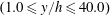 $(1.0\leqslant y/h\leqslant 40.0)$
a uniform streamwise velocity of
$(1.0\leqslant y/h\leqslant 40.0)$
a uniform streamwise velocity of
 $U_{\infty }=0.06U_{j}$
is defined as a co-flow. This co-flow provides entraining fluid and helps to avoid any large scale circulation in the computational domain. This co-flow is determined systematically using coarse grid simulations with decreasing co-flow magnitude and is lower than previous studies (Zhou et al.
Reference Zhou, Heine and Wygnanski1996; Ahlman et al.
Reference Ahlman, Brethouwer and Johansson2007).
$U_{\infty }=0.06U_{j}$
is defined as a co-flow. This co-flow provides entraining fluid and helps to avoid any large scale circulation in the computational domain. This co-flow is determined systematically using coarse grid simulations with decreasing co-flow magnitude and is lower than previous studies (Zhou et al.
Reference Zhou, Heine and Wygnanski1996; Ahlman et al.
Reference Ahlman, Brethouwer and Johansson2007).
At the bottom wall of the domain, the no-slip boundary condition is applied i.e.
 $u=v=w=0$
. The top wall of the domain has a shear free boundary condition, which is given as
$u=v=w=0$
. The top wall of the domain has a shear free boundary condition, which is given as
 $\unicode[STIX]{x2202}u/\unicode[STIX]{x2202}y=\unicode[STIX]{x2202}w/\unicode[STIX]{x2202}y=v=0$
. In the spanwise direction a periodic boundary condition is applied. At the exit plane, the convective outflow boundary condition of Orlanski (Reference Orlanski1976) is applied, which is given as
$\unicode[STIX]{x2202}u/\unicode[STIX]{x2202}y=\unicode[STIX]{x2202}w/\unicode[STIX]{x2202}y=v=0$
. In the spanwise direction a periodic boundary condition is applied. At the exit plane, the convective outflow boundary condition of Orlanski (Reference Orlanski1976) is applied, which is given as
 $\unicode[STIX]{x2202}u_{i}/\unicode[STIX]{x2202}t+U_{conv}(\unicode[STIX]{x2202}u_{i}/\unicode[STIX]{x2202}x)=0$
. The mean streamwise velocity profile at the exit plane is used as the convective velocity
$\unicode[STIX]{x2202}u_{i}/\unicode[STIX]{x2202}t+U_{conv}(\unicode[STIX]{x2202}u_{i}/\unicode[STIX]{x2202}x)=0$
. The mean streamwise velocity profile at the exit plane is used as the convective velocity
 $U_{conv}$
. This convective velocity is calculated as a running time average (Lund, Wu & Squires Reference Lund, Wu and Squires1998), where the initial transients have to be removed. Figure 2(c) shows a resulting outflow convective velocity
$U_{conv}$
. This convective velocity is calculated as a running time average (Lund, Wu & Squires Reference Lund, Wu and Squires1998), where the initial transients have to be removed. Figure 2(c) shows a resulting outflow convective velocity
 $U_{conv}$
profile at around
$U_{conv}$
profile at around
 $t^{\ast }=1200$
, which has become statistically steady.
$t^{\ast }=1200$
, which has become statistically steady.

Figure 3. Quantification of the grid resolution of the current simulations: (a) grid size
 $\unicode[STIX]{x0394}x^{+},\unicode[STIX]{x0394}y^{+}$
and
$\unicode[STIX]{x0394}x^{+},\unicode[STIX]{x0394}y^{+}$
and
 $\unicode[STIX]{x0394}z^{+}$
distribution along the streamwise direction in wall units, (b) contours of
$\unicode[STIX]{x0394}z^{+}$
distribution along the streamwise direction in wall units, (b) contours of
 $\unicode[STIX]{x0394}y^{+}$
, the dashed line indicates the location of jet half-width
$\unicode[STIX]{x0394}y^{+}$
, the dashed line indicates the location of jet half-width
 $y=y_{1/2}$
, (c) contours of mean grid size
$y=y_{1/2}$
, (c) contours of mean grid size
 $\unicode[STIX]{x1D6E5}=(\unicode[STIX]{x0394}x+\unicode[STIX]{x0394}y+\unicode[STIX]{x0394}z)/3.0$
with respect to the Kolmogorov length scale
$\unicode[STIX]{x1D6E5}=(\unicode[STIX]{x0394}x+\unicode[STIX]{x0394}y+\unicode[STIX]{x0394}z)/3.0$
with respect to the Kolmogorov length scale
 $\unicode[STIX]{x1D702}$
and (d) actual grid distribution in
$\unicode[STIX]{x1D702}$
and (d) actual grid distribution in
 $x{-}y$
plane with every 21st point in the streamwise and every 11th point in the wall-normal direction shown.
$x{-}y$
plane with every 21st point in the streamwise and every 11th point in the wall-normal direction shown.
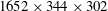
The simulation is performed with
 $1652\times 344\times 302$
grid points in the streamwise, wall-normal and spanwise directions, respectively, which results in approximately 172 million cells. This grid is mildly non-orthogonal and non-uniform in the
$1652\times 344\times 302$
grid points in the streamwise, wall-normal and spanwise directions, respectively, which results in approximately 172 million cells. This grid is mildly non-orthogonal and non-uniform in the
 $x{-}y$
plane, which follows the shear layer development. The grid is uniform in the spanwise direction. There are 78, 188 and 282 wall-normal points below
$x{-}y$
plane, which follows the shear layer development. The grid is uniform in the spanwise direction. There are 78, 188 and 282 wall-normal points below
 $y_{max}$
,
$y_{max}$
,
 $y_{1/2}$
and
$y_{1/2}$
and
 $2y_{1/2}$
, respectively. Figure 3(a) shows the streamwise
$2y_{1/2}$
, respectively. Figure 3(a) shows the streamwise
 $\unicode[STIX]{x0394}x^{+}$
, wall-normal
$\unicode[STIX]{x0394}x^{+}$
, wall-normal
 $\unicode[STIX]{x0394}y^{+}$
and spanwise
$\unicode[STIX]{x0394}y^{+}$
and spanwise
 $\unicode[STIX]{x0394}z^{+}$
grid size variations along the streamwise direction in wall units. The streamwise and spanwise grid sizes are in the range of
$\unicode[STIX]{x0394}z^{+}$
grid size variations along the streamwise direction in wall units. The streamwise and spanwise grid sizes are in the range of
 $5\leqslant \unicode[STIX]{x0394}x^{+}\leqslant 10.5$
and
$5\leqslant \unicode[STIX]{x0394}x^{+}\leqslant 10.5$
and
 $8\leqslant \unicode[STIX]{x0394}z^{+}\leqslant 12$
, respectively. The wall-normal distance of the first grid point is
$8\leqslant \unicode[STIX]{x0394}z^{+}\leqslant 12$
, respectively. The wall-normal distance of the first grid point is
 $\unicode[STIX]{x0394}y^{+}<0.7$
. In the near wall region there are
$\unicode[STIX]{x0394}y^{+}<0.7$
. In the near wall region there are
 $6$
points below
$6$
points below
 $y^{+}=5$
and
$y^{+}=5$
and
 $12$
points below
$12$
points below
 $y^{+}=11$
. Figure 3(b) shows the distribution of wall-normal grid size
$y^{+}=11$
. Figure 3(b) shows the distribution of wall-normal grid size
 $\unicode[STIX]{x0394}y^{+}$
, which is less than
$\unicode[STIX]{x0394}y^{+}$
, which is less than
 $6$
in the active flow region, particularly below the jet half-width
$6$
in the active flow region, particularly below the jet half-width
 $y/h<y_{1/2}$
. The grid size in wall units for the current simulation is comparable to previously reported DNS of wall jets (Ahlman et al.
Reference Ahlman, Brethouwer and Johansson2007; Pouransari et al.
Reference Pouransari, Vervisch and Johansson2014) and boundary layer flows (Schlatter et al.
Reference Schlatter, Orlu, Li, Brethouwer, Fransson, Johansson, Alfredsson and Henningson2009; Yuan & Piomelli Reference Yuan and Piomelli2015).
$y/h<y_{1/2}$
. The grid size in wall units for the current simulation is comparable to previously reported DNS of wall jets (Ahlman et al.
Reference Ahlman, Brethouwer and Johansson2007; Pouransari et al.
Reference Pouransari, Vervisch and Johansson2014) and boundary layer flows (Schlatter et al.
Reference Schlatter, Orlu, Li, Brethouwer, Fransson, Johansson, Alfredsson and Henningson2009; Yuan & Piomelli Reference Yuan and Piomelli2015).
For the DNS of any turbulent flow, the smallest resolved scale should be of the order of
 $O(\unicode[STIX]{x1D702})$
, where
$O(\unicode[STIX]{x1D702})$
, where
 $\unicode[STIX]{x1D702}=(\unicode[STIX]{x1D708}/\unicode[STIX]{x1D700})^{(1/4)}$
is the Kolmogorov length scale and
$\unicode[STIX]{x1D702}=(\unicode[STIX]{x1D708}/\unicode[STIX]{x1D700})^{(1/4)}$
is the Kolmogorov length scale and
 $\unicode[STIX]{x1D700}$
is the dissipation of turbulence kinetic energy (Moin & Mahesh Reference Moin and Mahesh1998). Figure 3(c) shows that the mean grid size with respect to the Kolmogorov length scale
$\unicode[STIX]{x1D700}$
is the dissipation of turbulence kinetic energy (Moin & Mahesh Reference Moin and Mahesh1998). Figure 3(c) shows that the mean grid size with respect to the Kolmogorov length scale
 $\unicode[STIX]{x1D6E5}/\unicode[STIX]{x1D702}$
is less than 6, where
$\unicode[STIX]{x1D6E5}/\unicode[STIX]{x1D702}$
is less than 6, where
 $\unicode[STIX]{x1D6E5}=(\unicode[STIX]{x0394}x+\unicode[STIX]{x0394}y+\unicode[STIX]{x0394}z)/3.0$
. The individual grid size in the streamwise, spanwise and wall-normal directions are
$\unicode[STIX]{x1D6E5}=(\unicode[STIX]{x0394}x+\unicode[STIX]{x0394}y+\unicode[STIX]{x0394}z)/3.0$
. The individual grid size in the streamwise, spanwise and wall-normal directions are
 $\unicode[STIX]{x0394}x/\unicode[STIX]{x1D702}<10$
,
$\unicode[STIX]{x0394}x/\unicode[STIX]{x1D702}<10$
,
 $\unicode[STIX]{x0394}z/\unicode[STIX]{x1D702}<10$
and
$\unicode[STIX]{x0394}z/\unicode[STIX]{x1D702}<10$
and
 $\unicode[STIX]{x0394}y/\unicode[STIX]{x1D702}<2$
, respectively. The current estimates of the grid resolution at the dissipation scales are comparable to the other studies reported in the literature e.g. Moser & Moin (Reference Moser and Moin1987), Yuan & Piomelli (Reference Yuan and Piomelli2015). Figure 3(d) shows the actual grid distribution.
$\unicode[STIX]{x0394}y/\unicode[STIX]{x1D702}<2$
, respectively. The current estimates of the grid resolution at the dissipation scales are comparable to the other studies reported in the literature e.g. Moser & Moin (Reference Moser and Moin1987), Yuan & Piomelli (Reference Yuan and Piomelli2015). Figure 3(d) shows the actual grid distribution.

Figure 4. Mean streamwise velocity and turbulent kinetic energy
 $(tke)$
profiles at
$(tke)$
profiles at
 $x=30.0h$
for coarse and fine grids: (a) outer scaling and (b) inner scaling.
$x=30.0h$
for coarse and fine grids: (a) outer scaling and (b) inner scaling.
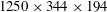
An initial simulation was performed with
 $1250\times 344\times 194$
grid points, totalling approximately 83 million cells. Figure 4 compares the mean streamwise velocity and turbulent kinetic energy (
$1250\times 344\times 194$
grid points, totalling approximately 83 million cells. Figure 4 compares the mean streamwise velocity and turbulent kinetic energy (
 $tke$
) profiles for the initial and final grids. The comparison is performed with both inner and outer scalings. The velocity profiles do not show any difference. The turbulent kinetic energy profiles have a maximum difference of 3 %. All the following results presented in this work are for the final, fine grid.
$tke$
) profiles for the initial and final grids. The comparison is performed with both inner and outer scalings. The velocity profiles do not show any difference. The turbulent kinetic energy profiles have a maximum difference of 3 %. All the following results presented in this work are for the final, fine grid.
A fixed time step based on the Courant–Friedrichs–Lewy (CFL) number is used, which is defined as
 $\unicode[STIX]{x0394}t((|u|/\unicode[STIX]{x0394}x)+(|v|/\unicode[STIX]{x0394}y)+(|w|/\unicode[STIX]{x0394}z))=0.5$
. This results in a maximum computational time step size of
$\unicode[STIX]{x0394}t((|u|/\unicode[STIX]{x0394}x)+(|v|/\unicode[STIX]{x0394}y)+(|w|/\unicode[STIX]{x0394}z))=0.5$
. This results in a maximum computational time step size of
 $\unicode[STIX]{x0394}t^{\ast }=0.0015$
. The simulation is initialized using a uniform flow field with
$\unicode[STIX]{x0394}t^{\ast }=0.0015$
. The simulation is initialized using a uniform flow field with
 $u=0.08$
,
$u=0.08$
,
 $v=0.0$
and
$v=0.0$
and
 $w=0.0$
, which is the streamwise bulk velocity at any
$w=0.0$
, which is the streamwise bulk velocity at any
 $y{-}z$
plane of the domain. The flow develops for
$y{-}z$
plane of the domain. The flow develops for
 $1200t^{\ast }$
to reach a statistically steady state and statistics are collected thereafter for a period of
$1200t^{\ast }$
to reach a statistically steady state and statistics are collected thereafter for a period of
 $1300t^{\ast }$
.
$1300t^{\ast }$
.

Figure 5. Iso-surfaces of the second invariant of the velocity gradient tensor in the wall jet. The iso-surfaces are coloured with the local streamwise velocity
 $u$
. The
$u$
. The
 $x{-}y$
plane shows the contours of spanwise averaged fluctuating pressure field
$x{-}y$
plane shows the contours of spanwise averaged fluctuating pressure field
 $\langle p^{\prime }\rangle _{z}$
and closed streamlines representing the footprint of large scale rotating structures.
$\langle p^{\prime }\rangle _{z}$
and closed streamlines representing the footprint of large scale rotating structures.
3 Results
3.1 Unsteady flow
There are not many examples available in the literature where large scale three-dimensional structures are presented for wall jets at higher Reynolds numbers. Banyassady & Piomelli (Reference Banyassady and Piomelli2014) used fluctuating pressure scaled with the maximum local velocity
 $p^{\prime }/\unicode[STIX]{x1D70C}U_{max}^{2}$
to visualize coherent structures in a wall jet at
$p^{\prime }/\unicode[STIX]{x1D70C}U_{max}^{2}$
to visualize coherent structures in a wall jet at
 $Re_{j}=7500$
. The fluctuating pressure contours in their simulation showed only large roll structures in the outer layer of the fully developed region of the wall jet. In this work, the
$Re_{j}=7500$
. The fluctuating pressure contours in their simulation showed only large roll structures in the outer layer of the fully developed region of the wall jet. In this work, the
 $Q$
-criterion will be used to identify the large scale structures, which is defined as the second invariant of the velocity gradient tensor
$Q$
-criterion will be used to identify the large scale structures, which is defined as the second invariant of the velocity gradient tensor
 $\unicode[STIX]{x1D735}\boldsymbol{u}$
.
$\unicode[STIX]{x1D735}\boldsymbol{u}$
.
Figure 5 shows an instantaneous picture of large scale vortical structures in the outer layer of the wall jet. Along the outer lip of the wall jet in the shear layer region for
 $x/h<3$
, Kelvin–Helmholtz instability generates roll structures, which are convected downstream. The roll structures interact with each other and breakdown into smaller more complex structures within a distance of
$x/h<3$
, Kelvin–Helmholtz instability generates roll structures, which are convected downstream. The roll structures interact with each other and breakdown into smaller more complex structures within a distance of
 $x/h=5$
from the inlet. These smaller structures undergo a complex motion and farther downstream for
$x/h=5$
from the inlet. These smaller structures undergo a complex motion and farther downstream for
 $x/h>20$
, structures have some large scale rotation. In order to identify this rotation, time averaged flow variables are subtracted from the instantaneous three-dimensional field shown in figure 5 and fluctuating flow variables are averaged in spanwise direction. Figure 5 shows an
$x/h>20$
, structures have some large scale rotation. In order to identify this rotation, time averaged flow variables are subtracted from the instantaneous three-dimensional field shown in figure 5 and fluctuating flow variables are averaged in spanwise direction. Figure 5 shows an
 $x{-}y$
plane, with the contours of spanwise averaged fluctuating pressure
$x{-}y$
plane, with the contours of spanwise averaged fluctuating pressure
 $\langle p^{\prime }\rangle _{z}$
field and streamlines based on spanwise averaged fluctuating velocities
$\langle p^{\prime }\rangle _{z}$
field and streamlines based on spanwise averaged fluctuating velocities
 $\langle u^{\prime }\rangle _{z}$
and
$\langle u^{\prime }\rangle _{z}$
and
 $\langle v^{\prime }\rangle _{z}$
. The streamlines form closed loops. On moving downstream, these grow in size and move away from the wall with the growth of the outer layer. These closed loop streamlines coincide with the peak values of pressure fluctuations
$\langle v^{\prime }\rangle _{z}$
. The streamlines form closed loops. On moving downstream, these grow in size and move away from the wall with the growth of the outer layer. These closed loop streamlines coincide with the peak values of pressure fluctuations
 $\langle p^{\prime }\rangle _{z}$
and represent the footprint of large scale rotation present in the outer shear layer. Banyassady & Piomelli (Reference Banyassady and Piomelli2014) used iso-surfaces of fluctuating pressure
$\langle p^{\prime }\rangle _{z}$
and represent the footprint of large scale rotation present in the outer shear layer. Banyassady & Piomelli (Reference Banyassady and Piomelli2014) used iso-surfaces of fluctuating pressure
 $p^{\prime }$
to identify large roll structures in the outer layer region far downstream beyond
$p^{\prime }$
to identify large roll structures in the outer layer region far downstream beyond
 $x/h>25$
, similar to the structures identified here.
$x/h>25$
, similar to the structures identified here.

Figure 6. Iso-surfaces of the second invariant of the velocity gradient tensor in the inner layer region of the wall jet. The iso-surfaces are coloured with the local streamwise velocity
 $u$
.
$u$
.
The near wall inner layer structures are made visible by blanking the flow field above
 $y/h=0.25$
. Figure 6 shows the instantaneous inner layer structures. The initial transition region for the inner layer stretches over the range
$y/h=0.25$
. Figure 6 shows the instantaneous inner layer structures. The initial transition region for the inner layer stretches over the range
 $0\leqslant x/h<15$
and the developed region extends beyond
$0\leqslant x/h<15$
and the developed region extends beyond
 $x/h>20$
. The transition region shows closely spaced patches of turbulence. These look identical to the turbulence spots appearing in transitional boundary layer flow (Wu & Moin Reference Wu and Moin2009). In the developed region, for
$x/h>20$
. The transition region shows closely spaced patches of turbulence. These look identical to the turbulence spots appearing in transitional boundary layer flow (Wu & Moin Reference Wu and Moin2009). In the developed region, for
 $x/h>20$
, more streamwise aligned tube-like structures appear.
$x/h>20$
, more streamwise aligned tube-like structures appear.

Figure 7. The decay of maximum mean streamwise velocity
 $U_{max}$
as a function of: (a) local streamwise distance from the jet inlet scaled with the slot height and (b) the local half-width
$U_{max}$
as a function of: (a) local streamwise distance from the jet inlet scaled with the slot height and (b) the local half-width
 $y_{1/2}$
normalized with the slot height. Current DNS (▫); power law fit to current DNS (——). LES of Banyassady & Piomelli (Reference Banyassady and Piomelli2014) (●). Experimental data: Tang et al. (Reference Tang, Rostamy, Bergstrom, Bugg and Sumner2015) (– – –); Barenblatt et al. (Reference Barenblatt, Chorin and Prostokishin2005) (— ⋅ ⋅ —); George et al. (Reference George, Abrahamsson, Eriksson, Karlsson, Lofdahal and Wosnik2000) (— ⋅ —).
$y_{1/2}$
normalized with the slot height. Current DNS (▫); power law fit to current DNS (——). LES of Banyassady & Piomelli (Reference Banyassady and Piomelli2014) (●). Experimental data: Tang et al. (Reference Tang, Rostamy, Bergstrom, Bugg and Sumner2015) (– – –); Barenblatt et al. (Reference Barenblatt, Chorin and Prostokishin2005) (— ⋅ ⋅ —); George et al. (Reference George, Abrahamsson, Eriksson, Karlsson, Lofdahal and Wosnik2000) (— ⋅ —).
3.2 Global properties
Figure 7(a) shows the decay of maximum mean streamwise velocity
 $U_{max}$
of the wall jet as a function of streamwise distance from the jet exit plane on a log–log scale. The current DNS is compared with the power law given by Barenblatt et al. (Reference Barenblatt, Chorin and Prostokishin2005) and Tang et al. (Reference Tang, Rostamy, Bergstrom, Bugg and Sumner2015). The power law is generally defined as
$U_{max}$
of the wall jet as a function of streamwise distance from the jet exit plane on a log–log scale. The current DNS is compared with the power law given by Barenblatt et al. (Reference Barenblatt, Chorin and Prostokishin2005) and Tang et al. (Reference Tang, Rostamy, Bergstrom, Bugg and Sumner2015). The power law is generally defined as
 $$\begin{eqnarray}\displaystyle \frac{U_{max}}{U_{j}}=A_{m}\left(\frac{x}{h}\right)^{\unicode[STIX]{x1D6FE}_{m}}. & & \displaystyle\end{eqnarray}$$
The exponents of the power law are given by Barenblatt et al. (Reference Barenblatt, Chorin and Prostokishin2005) and Tang et al. (Reference Tang, Rostamy, Bergstrom, Bugg and Sumner2015) as
 $\unicode[STIX]{x1D6FE}_{m}=-0.482$
and
$\unicode[STIX]{x1D6FE}_{m}=-0.482$
and
 $-0.6$
, respectively. The current DNS gives a value of
$-0.6$
, respectively. The current DNS gives a value of
 $\unicode[STIX]{x1D6FE}_{m}=-0.4907$
beyond
$\unicode[STIX]{x1D6FE}_{m}=-0.4907$
beyond
 $x/h=20$
, which is within the measured range. Previously it has been assumed that
$x/h=20$
, which is within the measured range. Previously it has been assumed that
 $\unicode[STIX]{x1D6FE}_{m}=-0.5$
(Launder & Rodi Reference Launder and Rodi1981; Wygnanski et al.
Reference Wygnanski, Katz and Horev1992). However, Wygnanski et al. (Reference Wygnanski, Katz and Horev1992) suggested that their experimental data fit the power law better when the exponent is
$\unicode[STIX]{x1D6FE}_{m}=-0.5$
(Launder & Rodi Reference Launder and Rodi1981; Wygnanski et al.
Reference Wygnanski, Katz and Horev1992). However, Wygnanski et al. (Reference Wygnanski, Katz and Horev1992) suggested that their experimental data fit the power law better when the exponent is
 $-0.47$
. This is within 2.5 % of the value given by Tang et al. (Reference Tang, Rostamy, Bergstrom, Bugg and Sumner2015). Narasimha, Narayan & Parthasarathy (Reference Narasimha, Narayan and Parthasarathy1973) reported
$-0.47$
. This is within 2.5 % of the value given by Tang et al. (Reference Tang, Rostamy, Bergstrom, Bugg and Sumner2015). Narasimha, Narayan & Parthasarathy (Reference Narasimha, Narayan and Parthasarathy1973) reported
 $4\leqslant A_{m}\leqslant 7$
and
$4\leqslant A_{m}\leqslant 7$
and
 $-0.62\leqslant \unicode[STIX]{x1D6FE}_{m}\leqslant -0.49$
. The maximum streamwise velocity values from the recent LES of Banyassady & Piomelli (Reference Banyassady and Piomelli2014) are included in figure 7(a). These are close to the current DNS. Barenblatt et al. (Reference Barenblatt, Chorin and Prostokishin2005) have argued that if
$-0.62\leqslant \unicode[STIX]{x1D6FE}_{m}\leqslant -0.49$
. The maximum streamwise velocity values from the recent LES of Banyassady & Piomelli (Reference Banyassady and Piomelli2014) are included in figure 7(a). These are close to the current DNS. Barenblatt et al. (Reference Barenblatt, Chorin and Prostokishin2005) have argued that if
 $\unicode[STIX]{x1D6FE}_{m}\neq -0.5$
, flow parameters have incomplete similarity or, in other words, they depend on the inlet slot height. However, current DNS and several other measurements give
$\unicode[STIX]{x1D6FE}_{m}\neq -0.5$
, flow parameters have incomplete similarity or, in other words, they depend on the inlet slot height. However, current DNS and several other measurements give
 $\unicode[STIX]{x1D6FE}_{m}$
close to
$\unicode[STIX]{x1D6FE}_{m}$
close to
 $-0.5$
. The value of
$-0.5$
. The value of
 $\unicode[STIX]{x1D6FE}_{m}=-0.6$
, given by Barenblatt et al. (Reference Barenblatt, Chorin and Prostokishin2005) is based on the data of Karlsson, Eriksson & Persson (Reference Karlsson, Eriksson and Persson1993), which might be affected by reverse flow (George et al.
Reference George, Abrahamsson, Eriksson, Karlsson, Lofdahal and Wosnik2000).
$\unicode[STIX]{x1D6FE}_{m}=-0.6$
, given by Barenblatt et al. (Reference Barenblatt, Chorin and Prostokishin2005) is based on the data of Karlsson, Eriksson & Persson (Reference Karlsson, Eriksson and Persson1993), which might be affected by reverse flow (George et al.
Reference George, Abrahamsson, Eriksson, Karlsson, Lofdahal and Wosnik2000).
Figure 7(b) shows the log–log plot of
 $U_{max}/U_{j}$
against
$U_{max}/U_{j}$
against
 $y_{1/2}/h$
. George et al. (Reference George, Abrahamsson, Eriksson, Karlsson, Lofdahal and Wosnik2000) noted that there is no theoretical justification for this normalization. However, data from several studies collapse to a power law given as
$y_{1/2}/h$
. George et al. (Reference George, Abrahamsson, Eriksson, Karlsson, Lofdahal and Wosnik2000) noted that there is no theoretical justification for this normalization. However, data from several studies collapse to a power law given as
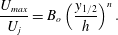 $$\begin{eqnarray}\displaystyle \frac{U_{max}}{U_{j}}=B_{o}\left(\frac{y_{1/2}}{h}\right)^{n}. & & \displaystyle\end{eqnarray}$$
The exponent of the power law in figure 7(b) is given as
 $n=-0.528$
and
$n=-0.528$
and
 $-0.524$
based on the measurements by George et al. (Reference George, Abrahamsson, Eriksson, Karlsson, Lofdahal and Wosnik2000) and Tang et al. (Reference Tang, Rostamy, Bergstrom, Bugg and Sumner2015), respectively. These values are within 0.8 % of each other. The power law defined by George et al. (Reference George, Abrahamsson, Eriksson, Karlsson, Lofdahal and Wosnik2000) relies on data for
$-0.524$
based on the measurements by George et al. (Reference George, Abrahamsson, Eriksson, Karlsson, Lofdahal and Wosnik2000) and Tang et al. (Reference Tang, Rostamy, Bergstrom, Bugg and Sumner2015), respectively. These values are within 0.8 % of each other. The power law defined by George et al. (Reference George, Abrahamsson, Eriksson, Karlsson, Lofdahal and Wosnik2000) relies on data for
 $x/h\geqslant 40$
and for the data of Tang et al. (Reference Tang, Rostamy, Bergstrom, Bugg and Sumner2015) it is valid for
$x/h\geqslant 40$
and for the data of Tang et al. (Reference Tang, Rostamy, Bergstrom, Bugg and Sumner2015) it is valid for
 $x/h\geqslant 30$
. However, the current DNS shows that it is in good agreement with these power laws at axial locations greater than
$x/h\geqslant 30$
. However, the current DNS shows that it is in good agreement with these power laws at axial locations greater than
 $x/h=25$
, with the values of
$x/h=25$
, with the values of
 $B_{o}=1.18$
and
$B_{o}=1.18$
and
 $n=-0.542$
.
$n=-0.542$
.

Figure 8. Streamwise development of the wall-normal location
 $y_{max}$
of
$y_{max}$
of
 $U_{max}$
. Current DNS (▫); power law fit to current DNS (——). Experimental data: Tang et al. (Reference Tang, Rostamy, Bergstrom, Bugg and Sumner2015) (– – –); Tachie, Balachandar & Bergstrom (Reference Tachie, Balachandar and Bergstrom2004), linear fit (— ⋅ —),
$U_{max}$
. Current DNS (▫); power law fit to current DNS (——). Experimental data: Tang et al. (Reference Tang, Rostamy, Bergstrom, Bugg and Sumner2015) (– – –); Tachie, Balachandar & Bergstrom (Reference Tachie, Balachandar and Bergstrom2004), linear fit (— ⋅ —),
 $Re=9100$
(▵),
$Re=9100$
(▵),
 $Re=6100$
(○).
$Re=6100$
(○).
Figure 8 shows the log–log plot of the streamwise variation of the wall-normal location
 $y_{max}$
of the maximum streamwise velocity. Tang et al. (Reference Tang, Rostamy, Bergstrom, Bugg and Sumner2015) defined a power-law relationship for
$y_{max}$
of the maximum streamwise velocity. Tang et al. (Reference Tang, Rostamy, Bergstrom, Bugg and Sumner2015) defined a power-law relationship for
 $y_{max}/h$
as
$y_{max}/h$
as
 $$\begin{eqnarray}\displaystyle \frac{y_{max}}{h}=B_{m}\left(\frac{x}{h}\right)^{m}. & & \displaystyle\end{eqnarray}$$
The accurate experimental measurement of
 $y_{max}$
is challenging. However, a power-law fit to the current DNS shows that it has the exponent
$y_{max}$
is challenging. However, a power-law fit to the current DNS shows that it has the exponent
 $m=-0.7403$
as compared to 0.717 measured by Tang et al. (Reference Tang, Rostamy, Bergstrom, Bugg and Sumner2015). The values of
$m=-0.7403$
as compared to 0.717 measured by Tang et al. (Reference Tang, Rostamy, Bergstrom, Bugg and Sumner2015). The values of
 $B_{m}$
are
$B_{m}$
are
 $0.0403$
and 0.040 for the DNS and experiment, respectively. Tachie et al. (Reference Tachie, Balachandar and Bergstrom2004) have also measured
$0.0403$
and 0.040 for the DNS and experiment, respectively. Tachie et al. (Reference Tachie, Balachandar and Bergstrom2004) have also measured
 $y_{max}$
for various inlet Reynolds numbers. The linear fit through their measurements is also included along with two of the representative values at
$y_{max}$
for various inlet Reynolds numbers. The linear fit through their measurements is also included along with two of the representative values at
 $Re=9100$
and 6100, shown by symbols. These are in agreement with the current DNS.
$Re=9100$
and 6100, shown by symbols. These are in agreement with the current DNS.

Figure 9. Wall jet spreading rate in (a) the outer layer and (b) the inner layer. Current DNS (▫); power law fit to current DNS (——). Experimental data: Tang et al. (Reference Tang, Rostamy, Bergstrom, Bugg and Sumner2015) (– – –); Launder & Rodi (Reference Launder and Rodi1981) (— ⋅ —); Eriksson et al. (Reference Eriksson, Karlsson and Persson1998) (— ⋅ ⋅ —).
Figure 9 shows the jet spreading rate (or the variation of jet half-width) in the inner and outer layers along the streamwise direction. Barenblatt et al. (Reference Barenblatt, Chorin and Prostokishin2005) have shown that the streamwise development of the half-width in the inner and outer layer regions follow independent scaling laws. The scaling power laws based on the jet slot height
 $h$
are defined as
$h$
are defined as
 $$\begin{eqnarray}\displaystyle \frac{y_{1/2}}{h}=A_{o}\left(\frac{x}{h}\right)^{\unicode[STIX]{x1D6FE}_{o}}\quad \text{(outer layer)}, & & \displaystyle\end{eqnarray}$$
and
 $$\begin{eqnarray}\displaystyle \frac{(y_{1/2})_{in}}{h}=A_{i}\left(\frac{x}{h}\right)^{\unicode[STIX]{x1D6FE}_{i}}\quad \text{(inner layer)}. & & \displaystyle\end{eqnarray}$$
The outer layer half-width
 $y_{1/2}$
is compared with the power law given by Tang et al. (Reference Tang, Rostamy, Bergstrom, Bugg and Sumner2015) based on their experimental data (figure 9
a). The power-law fit through the current DNS and Tang et al. (Reference Tang, Rostamy, Bergstrom, Bugg and Sumner2015) have the same exponent,
$y_{1/2}$
is compared with the power law given by Tang et al. (Reference Tang, Rostamy, Bergstrom, Bugg and Sumner2015) based on their experimental data (figure 9
a). The power-law fit through the current DNS and Tang et al. (Reference Tang, Rostamy, Bergstrom, Bugg and Sumner2015) have the same exponent,
 $\unicode[STIX]{x1D6FE}_{o}=0.78$
. This is 20 % lower than the value
$\unicode[STIX]{x1D6FE}_{o}=0.78$
. This is 20 % lower than the value
 $\unicode[STIX]{x1D6FE}_{o}=0.93$
reported by Barenblatt et al. (Reference Barenblatt, Chorin and Prostokishin2005). Other researchers have reported higher values for
$\unicode[STIX]{x1D6FE}_{o}=0.93$
reported by Barenblatt et al. (Reference Barenblatt, Chorin and Prostokishin2005). Other researchers have reported higher values for
 $\unicode[STIX]{x1D6FE}_{o}$
, for example, Narasimha et al. (Reference Narasimha, Narayan and Parthasarathy1973) gave
$\unicode[STIX]{x1D6FE}_{o}$
, for example, Narasimha et al. (Reference Narasimha, Narayan and Parthasarathy1973) gave
 $\unicode[STIX]{x1D6FE}_{o}=0.91$
and Wygnanski et al. (Reference Wygnanski, Katz and Horev1992) 0.88. The coefficient
$\unicode[STIX]{x1D6FE}_{o}=0.91$
and Wygnanski et al. (Reference Wygnanski, Katz and Horev1992) 0.88. The coefficient
 $A_{o}$
for Tang et al. (Reference Tang, Rostamy, Bergstrom, Bugg and Sumner2015) is 0.230, which is significantly higher than 0.175 for the current DNS. The measured values of
$A_{o}$
for Tang et al. (Reference Tang, Rostamy, Bergstrom, Bugg and Sumner2015) is 0.230, which is significantly higher than 0.175 for the current DNS. The measured values of
 $y_{1/2}$
are hence greater than the DNS. Linear relationships for half-width have also been defined as
$y_{1/2}$
are hence greater than the DNS. Linear relationships for half-width have also been defined as
 $y_{1/2}/h=0.0732(x/h)+0.332$
(Launder & Rodi Reference Launder and Rodi1981) and
$y_{1/2}/h=0.0732(x/h)+0.332$
(Launder & Rodi Reference Launder and Rodi1981) and
 $y_{1/2}/h=0.0782(x/h)+0.332$
(Eriksson et al.
Reference Eriksson, Karlsson and Persson1998), which are closer to the current DNS than the measurements of Tang et al. (Reference Tang, Rostamy, Bergstrom, Bugg and Sumner2015). The average value of the ratio
$y_{1/2}/h=0.0782(x/h)+0.332$
(Eriksson et al.
Reference Eriksson, Karlsson and Persson1998), which are closer to the current DNS than the measurements of Tang et al. (Reference Tang, Rostamy, Bergstrom, Bugg and Sumner2015). The average value of the ratio
 $y_{max}/y_{1/2}$
for
$y_{max}/y_{1/2}$
for
 $25\leqslant x/h\leqslant 40$
is given by current DNS as 0.2, which is higher than a previously reported value of 0.17 (Karlsson et al.
Reference Karlsson, Eriksson and Persson1993).
$25\leqslant x/h\leqslant 40$
is given by current DNS as 0.2, which is higher than a previously reported value of 0.17 (Karlsson et al.
Reference Karlsson, Eriksson and Persson1993).
Figure 9(b) compares the inner layer half-width
 $(y_{1/2})_{in}$
from the DNS with the power law given by Tang et al. (Reference Tang, Rostamy, Bergstrom, Bugg and Sumner2015). The power-law fit through the DNS data has the same exponent
$(y_{1/2})_{in}$
from the DNS with the power law given by Tang et al. (Reference Tang, Rostamy, Bergstrom, Bugg and Sumner2015). The power-law fit through the DNS data has the same exponent
 $\unicode[STIX]{x1D6FE}_{i}=0.504$
as the measurements (Tang et al.
Reference Tang, Rostamy, Bergstrom, Bugg and Sumner2015). Barenblatt et al. (Reference Barenblatt, Chorin and Prostokishin2005) gave the power-law exponent
$\unicode[STIX]{x1D6FE}_{i}=0.504$
as the measurements (Tang et al.
Reference Tang, Rostamy, Bergstrom, Bugg and Sumner2015). Barenblatt et al. (Reference Barenblatt, Chorin and Prostokishin2005) gave the power-law exponent
 $\unicode[STIX]{x1D6FE}_{i}=0.68$
, which is 20 % higher than the current value. The coefficient
$\unicode[STIX]{x1D6FE}_{i}=0.68$
, which is 20 % higher than the current value. The coefficient
 $A_{i}=0.005$
for the DNS is lower than the measured value of 0.007 (Tang et al.
Reference Tang, Rostamy, Bergstrom, Bugg and Sumner2015). The measured data hence produce higher values of
$A_{i}=0.005$
for the DNS is lower than the measured value of 0.007 (Tang et al.
Reference Tang, Rostamy, Bergstrom, Bugg and Sumner2015). The measured data hence produce higher values of
 $(y_{1/2})_{in}$
than the DNS.
$(y_{1/2})_{in}$
than the DNS.

Figure 10. (a) Streamwise development of the wall shear stress scaled with momentum–viscosity scaling. Current DNS (▫); power law fit to current DNS (——). LES of Banyassady & Piomelli (Reference Banyassady and Piomelli2014) (●). Experimental data: Rostamy et al. (Reference Rostamy, Bergstrom, Sumner and Bugg2011b
) (– – –); Wygnanski et al. (Reference Wygnanski, Katz and Horev1992) (— ⋅ —). (b) Variation of skin friction coefficient
 $C_{f}$
with local Reynolds number
$C_{f}$
with local Reynolds number
 $Re_{m}=U_{max}y_{max}/\unicode[STIX]{x1D708}$
. Current DNS (▫). LES of Banyassady & Piomelli (Reference Banyassady and Piomelli2015) (●). Experimental data: Eriksson et al. (Reference Eriksson, Karlsson and Persson1998) (▵); Tachie et al. (Reference Tachie, Balachandar and Bergstrom2004) (▿); Rostamy et al. (Reference Rostamy, Bergstrom, Sumner and Bugg2011b
) (○); George et al. (Reference George, Abrahamsson, Eriksson, Karlsson, Lofdahal and Wosnik2000) (— ⋅ ⋅ —).
$Re_{m}=U_{max}y_{max}/\unicode[STIX]{x1D708}$
. Current DNS (▫). LES of Banyassady & Piomelli (Reference Banyassady and Piomelli2015) (●). Experimental data: Eriksson et al. (Reference Eriksson, Karlsson and Persson1998) (▵); Tachie et al. (Reference Tachie, Balachandar and Bergstrom2004) (▿); Rostamy et al. (Reference Rostamy, Bergstrom, Sumner and Bugg2011b
) (○); George et al. (Reference George, Abrahamsson, Eriksson, Karlsson, Lofdahal and Wosnik2000) (— ⋅ ⋅ —).
Figure 10(a) shows the streamwise evolution of wall shear stress
 $\unicode[STIX]{x1D70F}_{w}=\unicode[STIX]{x1D707}\unicode[STIX]{x2202}u/\unicode[STIX]{x2202}y|_{y=0}$
, where
$\unicode[STIX]{x1D70F}_{w}=\unicode[STIX]{x1D707}\unicode[STIX]{x2202}u/\unicode[STIX]{x2202}y|_{y=0}$
, where
 $\unicode[STIX]{x1D707}$
is the dynamic viscosity of the fluid. The scaling used here is defined by Narasimha et al. (Reference Narasimha, Narayan and Parthasarathy1973), which uses the initial kinetic momentum flux
$\unicode[STIX]{x1D707}$
is the dynamic viscosity of the fluid. The scaling used here is defined by Narasimha et al. (Reference Narasimha, Narayan and Parthasarathy1973), which uses the initial kinetic momentum flux
 $M_{o}=\int _{0}^{h}{U_{j}}^{2}\,\text{d}y$
, kinematic viscosity and density to scale wall shear stress. This approach eliminates the effect of inflow Reynolds number
$M_{o}=\int _{0}^{h}{U_{j}}^{2}\,\text{d}y$
, kinematic viscosity and density to scale wall shear stress. This approach eliminates the effect of inflow Reynolds number
 $Re_{j}$
on the scaling. The power-law form for this scaling is given as
$Re_{j}$
on the scaling. The power-law form for this scaling is given as
 $$\begin{eqnarray}\displaystyle \frac{\unicode[STIX]{x1D70F}_{w}\unicode[STIX]{x1D708}^{2}}{\unicode[STIX]{x1D70C}{M_{o}}^{2}}=A_{\unicode[STIX]{x1D70F}}\left(\frac{xM_{o}}{\unicode[STIX]{x1D708}^{2}}\right)^{\unicode[STIX]{x1D6FE}_{\unicode[STIX]{x1D70F}}}. & & \displaystyle\end{eqnarray}$$
The exponent for the power-law fit through the current DNS is
 $\unicode[STIX]{x1D6FE}_{\unicode[STIX]{x1D70F}}=-0.967$
. The value of
$\unicode[STIX]{x1D6FE}_{\unicode[STIX]{x1D70F}}=-0.967$
. The value of
 $\unicode[STIX]{x1D6FE}_{\unicode[STIX]{x1D70F}}$
based on measurements is given as
$\unicode[STIX]{x1D6FE}_{\unicode[STIX]{x1D70F}}$
based on measurements is given as
 $-1.053$
and
$-1.053$
and
 $-1.07$
by Rostamy et al. (Reference Rostamy, Bergstrom, Sumner and Bugg2011b
) and Wygnanski et al. (Reference Wygnanski, Katz and Horev1992), respectively. These values are within 10 % of each other. The coefficient
$-1.07$
by Rostamy et al. (Reference Rostamy, Bergstrom, Sumner and Bugg2011b
) and Wygnanski et al. (Reference Wygnanski, Katz and Horev1992), respectively. These values are within 10 % of each other. The coefficient
 $A_{\unicode[STIX]{x1D70F}}$
is determined to be 0.03, 0.161 and 0.146 for the current DNS, Rostamy et al. (Reference Rostamy, Bergstrom, Sumner and Bugg2011b
) and Wygnanski et al. (Reference Wygnanski, Katz and Horev1992), respectively. The wall shear stress predicted with LES (Banyassady & Piomelli Reference Banyassady and Piomelli2014) is close to the current DNS.
$A_{\unicode[STIX]{x1D70F}}$
is determined to be 0.03, 0.161 and 0.146 for the current DNS, Rostamy et al. (Reference Rostamy, Bergstrom, Sumner and Bugg2011b
) and Wygnanski et al. (Reference Wygnanski, Katz and Horev1992), respectively. The wall shear stress predicted with LES (Banyassady & Piomelli Reference Banyassady and Piomelli2014) is close to the current DNS.
Table 1. Various power laws for wall jets.

Figure 10(b) shows the log–log plot of skin friction coefficient
 $C_{f}$
against local Reynolds number
$C_{f}$
against local Reynolds number
 $Re_{m}=(U_{max}y_{max})/\unicode[STIX]{x1D708}$
.
$Re_{m}=(U_{max}y_{max})/\unicode[STIX]{x1D708}$
.
 $C_{f}$
is defined as
$C_{f}$
is defined as
 $$\begin{eqnarray}\displaystyle C_{f}=2\frac{\unicode[STIX]{x1D70F}_{w}}{\unicode[STIX]{x1D70C}U_{max}^{2}}=2\left(\frac{u_{\unicode[STIX]{x1D70F}}}{U_{max}}\right)^{2}. & & \displaystyle\end{eqnarray}$$
The local Reynolds number
 $Re_{m}$
in the developed region ranges from 2500 to 3100 for the current DNS. The predicted values of
$Re_{m}$
in the developed region ranges from 2500 to 3100 for the current DNS. The predicted values of
 $C_{f}$
are in agreement with several experimental studies (Eriksson et al.
Reference Eriksson, Karlsson and Persson1998; Tachie et al.
Reference Tachie, Balachandar and Bergstrom2004; Rostamy et al.
Reference Rostamy, Bergstrom, Sumner and Bugg2011b
). George et al. (Reference George, Abrahamsson, Eriksson, Karlsson, Lofdahal and Wosnik2000) gave a theoretical relation for friction velocity based on a power law. This can be used to determine the skin friction coefficient variation against
$C_{f}$
are in agreement with several experimental studies (Eriksson et al.
Reference Eriksson, Karlsson and Persson1998; Tachie et al.
Reference Tachie, Balachandar and Bergstrom2004; Rostamy et al.
Reference Rostamy, Bergstrom, Sumner and Bugg2011b
). George et al. (Reference George, Abrahamsson, Eriksson, Karlsson, Lofdahal and Wosnik2000) gave a theoretical relation for friction velocity based on a power law. This can be used to determine the skin friction coefficient variation against
 $Re_{m}$
. This relationship is also included in figure 10(b). The current DNS approaches it asymptotically beyond
$Re_{m}$
. This relationship is also included in figure 10(b). The current DNS approaches it asymptotically beyond
 $Re_{m}=2800$
. Banyassady & Piomelli (Reference Banyassady and Piomelli2015) have reported
$Re_{m}=2800$
. Banyassady & Piomelli (Reference Banyassady and Piomelli2015) have reported
 $C_{f}$
for a significantly longer range of
$C_{f}$
for a significantly longer range of
 $Re_{m}$
based on their LES, however, their reported values are higher than the current predictions.
$Re_{m}$
based on their LES, however, their reported values are higher than the current predictions.
Various power laws for the wall jet discussed in this section are summarized in table 1.
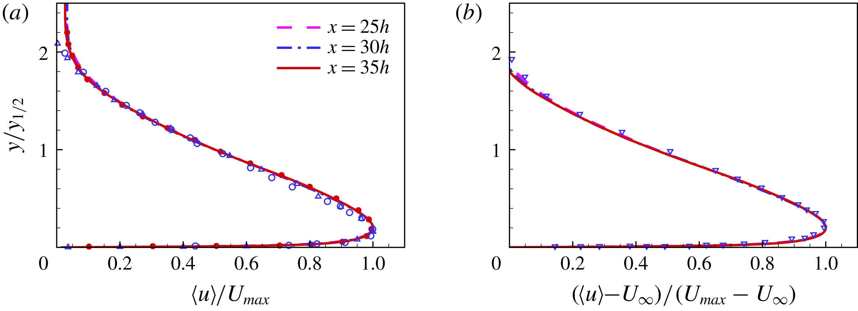
Figure 11. Mean streamwise velocity profiles scaled with outer length scales (a)
 $\langle u\rangle /U_{max}$
and (b)
$\langle u\rangle /U_{max}$
and (b)
 $(\langle u\rangle -U_{\infty })/(U_{max}-U_{\infty })$
. LES of Banyassady & Piomelli (Reference Banyassady and Piomelli2014) (●),
$(\langle u\rangle -U_{\infty })/(U_{max}-U_{\infty })$
. LES of Banyassady & Piomelli (Reference Banyassady and Piomelli2014) (●),
 $x=30h$
. Experimental data: Rostamy et al. (Reference Rostamy, Bergstrom, Sumner and Bugg2011a
) (○),
$x=30h$
. Experimental data: Rostamy et al. (Reference Rostamy, Bergstrom, Sumner and Bugg2011a
) (○),
 $x=30h$
; Eriksson et al. (Reference Eriksson, Karlsson and Persson1998) (▵),
$x=30h$
; Eriksson et al. (Reference Eriksson, Karlsson and Persson1998) (▵),
 $x=40h$
; Irwin (Reference Irwin1973) (▿),
$x=40h$
; Irwin (Reference Irwin1973) (▿),
 $x=82.2h$
.
$x=82.2h$
.
3.3 Mean flow and turbulence statistics
3.3.1 Mean velocity
Figure 11(a) shows mean streamwise velocity profiles at
 $x/h=25$
, 30 and 35. The profiles are scaled with the outer parameters
$x/h=25$
, 30 and 35. The profiles are scaled with the outer parameters
 $y_{1/2}$
and
$y_{1/2}$
and
 $U_{max}$
. For the given range in the streamwise direction, the profiles show self-similar behaviour. Eriksson et al. (Reference Eriksson, Karlsson and Persson1998) showed that the mean streamwise velocity profiles show self-similar behaviour in outer scales beyond
$U_{max}$
. For the given range in the streamwise direction, the profiles show self-similar behaviour. Eriksson et al. (Reference Eriksson, Karlsson and Persson1998) showed that the mean streamwise velocity profiles show self-similar behaviour in outer scales beyond
 $x/h=20$
. The mean flow predicted by previous LES (Banyassady & Piomelli Reference Banyassady and Piomelli2014) is in agreement with the DNS. The current results also compare well with the measurements of Rostamy et al. (Reference Rostamy, Bergstrom, Sumner and Bugg2011a
) and Eriksson et al. (Reference Eriksson, Karlsson and Persson1998). This is with the exception of close to the edge of outer layer beyond
$x/h=20$
. The mean flow predicted by previous LES (Banyassady & Piomelli Reference Banyassady and Piomelli2014) is in agreement with the DNS. The current results also compare well with the measurements of Rostamy et al. (Reference Rostamy, Bergstrom, Sumner and Bugg2011a
) and Eriksson et al. (Reference Eriksson, Karlsson and Persson1998). This is with the exception of close to the edge of outer layer beyond
 $y/y_{1/2}>1.8$
. This is due to the difference in outer flow conditions. The experiments have reverse flow for entrainment.
$y/y_{1/2}>1.8$
. This is due to the difference in outer flow conditions. The experiments have reverse flow for entrainment.
In the presence of a weak co-flow with the velocity
 $U_{\infty }$
, the outer scaling for the mean streamwise velocity is defined as
$U_{\infty }$
, the outer scaling for the mean streamwise velocity is defined as
 $(\langle u\rangle -U_{\infty })/(U_{max}-U_{\infty })$
(Irwin Reference Irwin1973; Zhou et al.
Reference Zhou, Heine and Wygnanski1996) and
$(\langle u\rangle -U_{\infty })/(U_{max}-U_{\infty })$
(Irwin Reference Irwin1973; Zhou et al.
Reference Zhou, Heine and Wygnanski1996) and
 $y_{1/2}$
is located where
$y_{1/2}$
is located where
 $\langle u\rangle =(1/2)(U_{max}-U_{\infty })$
. Figure 11(b) shows that the mean streamwise velocity profiles at
$\langle u\rangle =(1/2)(U_{max}-U_{\infty })$
. Figure 11(b) shows that the mean streamwise velocity profiles at
 $x/h=25$
,
$x/h=25$
,
 $30$
and
$30$
and
 $35$
collapse with this scaling in the outer layer region. The velocity profiles are compared with the experimental data of Irwin (Reference Irwin1973) at
$35$
collapse with this scaling in the outer layer region. The velocity profiles are compared with the experimental data of Irwin (Reference Irwin1973) at
 $Re_{j}=28\,000$
with
$Re_{j}=28\,000$
with
 $U_{\infty }/U_{max}=0.38$
.
$U_{\infty }/U_{max}=0.38$
.
Figure 12 shows the outer-scaled mean wall-normal velocity
 $\langle v\rangle$
. The velocity profiles do not collapse beyond
$\langle v\rangle$
. The velocity profiles do not collapse beyond
 $y/y_{1/2}=1.2$
. The calculated wall-normal velocity is in good agreement with the measurements of Eriksson et al. (Reference Eriksson, Karlsson and Persson1998) up to
$y/y_{1/2}=1.2$
. The calculated wall-normal velocity is in good agreement with the measurements of Eriksson et al. (Reference Eriksson, Karlsson and Persson1998) up to
 $y/y_{1/2}=1.6$
. The difference in measurements and computed values in the outer region is again due to different entrainment conditions.
$y/y_{1/2}=1.6$
. The difference in measurements and computed values in the outer region is again due to different entrainment conditions.

Figure 12. Mean wall-normal velocity profiles scaled with outer parameters. Experimental data: Eriksson et al. (Reference Eriksson, Karlsson and Persson1998) (▵),
 $x=70h$
.
$x=70h$
.

Figure 13. Inner-scaled mean streamwise velocity profiles
 $\langle u\rangle ^{+}$
. Log-law
$\langle u\rangle ^{+}$
. Log-law
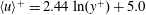 $\langle u\rangle ^{+}=2.44\ln (y^{+})+5.0$
(— ⋅ ⋅ —). Linear profile
$\langle u\rangle ^{+}=2.44\ln (y^{+})+5.0$
(— ⋅ ⋅ —). Linear profile
 $\langle u\rangle ^{+}=y^{+}$
(
$\langle u\rangle ^{+}=y^{+}$
(
 $\cdots \cdots$
). LES of Banyassady & Piomelli (Reference Banyassady and Piomelli2014) (●),
$\cdots \cdots$
). LES of Banyassady & Piomelli (Reference Banyassady and Piomelli2014) (●),
 $x=30h$
. Experimental data: Rostamy et al. (Reference Rostamy, Bergstrom, Sumner and Bugg2011a
) (○),
$x=30h$
. Experimental data: Rostamy et al. (Reference Rostamy, Bergstrom, Sumner and Bugg2011a
) (○),
 $x=30h$
; Eriksson et al. (Reference Eriksson, Karlsson and Persson1998) (▵),
$x=30h$
; Eriksson et al. (Reference Eriksson, Karlsson and Persson1998) (▵),
 $x=40h$
.
$x=40h$
.
Figure 13 shows the inner-scaled mean streamwise velocity
 $\langle u\rangle ^{+}$
profiles in a semi-logarithmic form. The computed profiles at three streamwise locations
$\langle u\rangle ^{+}$
profiles in a semi-logarithmic form. The computed profiles at three streamwise locations
 $x/h=25$
, 30 and 45 collapse up to
$x/h=25$
, 30 and 45 collapse up to
 $y^{+}=300$
. The current DNS is in agreement with the experimental data (Eriksson et al.
Reference Eriksson, Karlsson and Persson1998; Rostamy et al.
Reference Rostamy, Bergstrom, Sumner and Bugg2011a
). The LES of Banyassady & Piomelli (Reference Banyassady and Piomelli2014) gives slightly lower values for
$y^{+}=300$
. The current DNS is in agreement with the experimental data (Eriksson et al.
Reference Eriksson, Karlsson and Persson1998; Rostamy et al.
Reference Rostamy, Bergstrom, Sumner and Bugg2011a
). The LES of Banyassady & Piomelli (Reference Banyassady and Piomelli2014) gives slightly lower values for
 $\langle u\rangle ^{+}$
in the range of
$\langle u\rangle ^{+}$
in the range of
 $10\leqslant y^{+}\leqslant 370$
, than the current DNS. There is agreement with the linear profile
$10\leqslant y^{+}\leqslant 370$
, than the current DNS. There is agreement with the linear profile
 $\langle u\rangle ^{+}=y^{+}$
below
$\langle u\rangle ^{+}=y^{+}$
below
 $y^{+}=4$
, which is similar to the flat plate turbulent boundary layer (Wu & Moin Reference Wu and Moin2009). The near wall velocity profiles for wall bounded flows are also expressed as a log law of the form
$y^{+}=4$
, which is similar to the flat plate turbulent boundary layer (Wu & Moin Reference Wu and Moin2009). The near wall velocity profiles for wall bounded flows are also expressed as a log law of the form
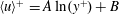 $\langle u\rangle ^{+}=A\ln (y^{+})+B$
. The current DNS is compared with a log law having
$\langle u\rangle ^{+}=A\ln (y^{+})+B$
. The current DNS is compared with a log law having
 $A=2.44$
and
$A=2.44$
and
 $B=5.0$
. These constants are the generally accepted values for flat plate turbulent boundary layers (Spalart Reference Spalart1988). Several previous experimental measurements of wall jets (Eriksson et al.
Reference Eriksson, Karlsson and Persson1998; Tachie et al.
Reference Tachie, Balachandar and Bergstrom2004; Rostamy et al.
Reference Rostamy, Bergstrom, Sumner and Bugg2011a
) have shown agreement with these log-law parameters. Eriksson et al. (Reference Eriksson, Karlsson and Persson1998) showed that their measurements are in agreement with the log law in the range of
$B=5.0$
. These constants are the generally accepted values for flat plate turbulent boundary layers (Spalart Reference Spalart1988). Several previous experimental measurements of wall jets (Eriksson et al.
Reference Eriksson, Karlsson and Persson1998; Tachie et al.
Reference Tachie, Balachandar and Bergstrom2004; Rostamy et al.
Reference Rostamy, Bergstrom, Sumner and Bugg2011a
) have shown agreement with these log-law parameters. Eriksson et al. (Reference Eriksson, Karlsson and Persson1998) showed that their measurements are in agreement with the log law in the range of
 $30\leqslant y^{+}\leqslant 80$
, whereas the current DNS range is
$30\leqslant y^{+}\leqslant 80$
, whereas the current DNS range is
 $20\leqslant y^{+}\leqslant 90$
. The log-law parameters for the LES (Banyassady & Piomelli Reference Banyassady and Piomelli2014) are
$20\leqslant y^{+}\leqslant 90$
. The log-law parameters for the LES (Banyassady & Piomelli Reference Banyassady and Piomelli2014) are
 $A=2.22$
and
$A=2.22$
and
 $B=5.0$
.
$B=5.0$
.

Figure 14. Mean streamwise velocity profiles scaled with incomplete similarity parameters of Barenblatt et al. (Reference Barenblatt, Chorin and Prostokishin2005): (a) outer scaled profiles and (b) inner-scaled profiles.
Figure 14 represents mean streamwise velocity profiles with incomplete similarity parameters described by Barenblatt et al. (Reference Barenblatt, Chorin and Prostokishin2005). The outer scaling parameters for incomplete similarity are traditionally defined except for the factor
 $A_{o}$
used for scaling the
$A_{o}$
used for scaling the
 $y$
-axis (figure 14
a). The parameter
$y$
-axis (figure 14
a). The parameter
 $A_{o}$
is given in (3.4), which describes the dependence of the outer layer length scale
$A_{o}$
is given in (3.4), which describes the dependence of the outer layer length scale
 $y_{1/2}$
on the streamwise distance
$y_{1/2}$
on the streamwise distance
 $x/h$
. The semi-logarithmic plot clearly shows that outer scale mean streamwise velocity profiles above
$x/h$
. The semi-logarithmic plot clearly shows that outer scale mean streamwise velocity profiles above
 $y_{max}$
show perfect collapse, whereas profiles below
$y_{max}$
show perfect collapse, whereas profiles below
 $y_{max}$
diverge. Figure 14(b) shows the inner-scaled profiles of mean streamwise velocity. The
$y_{max}$
diverge. Figure 14(b) shows the inner-scaled profiles of mean streamwise velocity. The
 $y$
-axis is scaled with
$y$
-axis is scaled with
 $A_{i}$
and
$A_{i}$
and
 $(y_{1/2})_{in}$
given in (3.5). The inner scaling is able to collapse the velocity profile in the inner layer region below
$(y_{1/2})_{in}$
given in (3.5). The inner scaling is able to collapse the velocity profile in the inner layer region below
 $y_{max}$
. Barenblatt et al. (Reference Barenblatt, Chorin and Prostokishin2005) gave a relationship for mean streamwise velocity based on incomplete similarity as
$y_{max}$
. Barenblatt et al. (Reference Barenblatt, Chorin and Prostokishin2005) gave a relationship for mean streamwise velocity based on incomplete similarity as
 $$\begin{eqnarray}\displaystyle \langle u\rangle =\left\{\begin{array}{@{}ll@{}}\displaystyle \left(\frac{M}{\unicode[STIX]{x1D70C}h}\right)^{1/2}\left(\frac{x}{h}\right)^{\unicode[STIX]{x1D6FE}_{m}}\unicode[STIX]{x1D713}_{u}\left(\frac{y}{h^{1-\unicode[STIX]{x1D6FE}_{o}}x^{\unicode[STIX]{x1D6FE}_{o}}},Re\right),\quad & \text{if }y>y_{max};\\ \displaystyle \left(\frac{M}{\unicode[STIX]{x1D70C}h}\right)^{1/2}\left(\frac{x}{h}\right)^{\unicode[STIX]{x1D6FE}_{m}}\unicode[STIX]{x1D713}_{u}\left(\frac{y}{h^{1-\unicode[STIX]{x1D6FE}_{i}}x^{\unicode[STIX]{x1D6FE}_{i}}},Re\right),\quad & \text{if }y<y_{max}.\end{array}\right. & & \displaystyle\end{eqnarray}$$
 $\unicode[STIX]{x1D713}_{u}$
is a function of length scales and Reynolds number. Earlier it was shown that the current DNS and several recent measurements give
$\unicode[STIX]{x1D713}_{u}$
is a function of length scales and Reynolds number. Earlier it was shown that the current DNS and several recent measurements give
 $\unicode[STIX]{x1D6FE}_{m}$
close to
$\unicode[STIX]{x1D6FE}_{m}$
close to
 $-0.5$
, which results in a weak dependence on inlet slot height and hence at high Reynolds number complete similarity is possible. It is important to point out that even if the hypothesis of incomplete similarity is not applicable for the wall jet, the inner layer parameters of (3.5) suggested by Barenblatt et al. (Reference Barenblatt, Chorin and Prostokishin2005) show the same quality of scaling as the inner scaling suggested by George et al. (Reference George, Abrahamsson, Eriksson, Karlsson, Lofdahal and Wosnik2000), based on the asymptotic invariance principle (AIP). It can be shown that the parameters given in (3.5) are consistent with the similarity theory of George et al. (Reference George, Abrahamsson, Eriksson, Karlsson, Lofdahal and Wosnik2000). The detailed derivation is given in George et al. (Reference George, Abrahamsson, Eriksson, Karlsson, Lofdahal and Wosnik2000), here the essential relationships are referenced to check the scaling parameters. It has been shown (George et al.
Reference George, Abrahamsson, Eriksson, Karlsson, Lofdahal and Wosnik2000) that at infinite Reynolds number the momentum equation in the inner layer region is given as
$-0.5$
, which results in a weak dependence on inlet slot height and hence at high Reynolds number complete similarity is possible. It is important to point out that even if the hypothesis of incomplete similarity is not applicable for the wall jet, the inner layer parameters of (3.5) suggested by Barenblatt et al. (Reference Barenblatt, Chorin and Prostokishin2005) show the same quality of scaling as the inner scaling suggested by George et al. (Reference George, Abrahamsson, Eriksson, Karlsson, Lofdahal and Wosnik2000), based on the asymptotic invariance principle (AIP). It can be shown that the parameters given in (3.5) are consistent with the similarity theory of George et al. (Reference George, Abrahamsson, Eriksson, Karlsson, Lofdahal and Wosnik2000). The detailed derivation is given in George et al. (Reference George, Abrahamsson, Eriksson, Karlsson, Lofdahal and Wosnik2000), here the essential relationships are referenced to check the scaling parameters. It has been shown (George et al.
Reference George, Abrahamsson, Eriksson, Karlsson, Lofdahal and Wosnik2000) that at infinite Reynolds number the momentum equation in the inner layer region is given as
 $$\begin{eqnarray}\displaystyle \frac{\unicode[STIX]{x2202}}{\unicode[STIX]{x2202}y}\left[\langle -u^{\prime }v^{\prime }\rangle +\unicode[STIX]{x1D708}\frac{\unicode[STIX]{x2202}\langle u\rangle }{\unicode[STIX]{x2202}y}\right]=0, & & \displaystyle\end{eqnarray}$$
where
 $\langle u\rangle =0$
at
$\langle u\rangle =0$
at
 $y=0$
. Equation (3.9) can be integrated to obtain
$y=0$
. Equation (3.9) can be integrated to obtain
 $$\begin{eqnarray}\displaystyle \langle -u^{\prime }v^{\prime }\rangle +\unicode[STIX]{x1D708}\frac{\unicode[STIX]{x2202}\langle u\rangle }{\unicode[STIX]{x2202}y}=\frac{\unicode[STIX]{x1D70F}_{w}}{\unicode[STIX]{x1D70C}}=u_{\unicode[STIX]{x1D70F}}. & & \displaystyle\end{eqnarray}$$
The form of similarity solution is given as
 $$\begin{eqnarray}\displaystyle & \displaystyle \langle u\rangle =U_{si}(x)f_{i\infty }(y_{si}), & \displaystyle\end{eqnarray}$$
 $$\begin{eqnarray}\displaystyle & \displaystyle \langle -u^{\prime }v^{\prime }\rangle =R_{si}(x)r_{i\infty }(y_{si}), & \displaystyle\end{eqnarray}$$
where
 $U_{si}$
,
$U_{si}$
,
 $f_{i\infty }$
,
$f_{i\infty }$
,
 $R_{si}$
and
$R_{si}$
and
 $r_{i\infty }$
are spatial functions.
$r_{i\infty }$
are spatial functions.
 $y_{si}=y/l_{si}$
and length scale
$y_{si}=y/l_{si}$
and length scale
 $l_{si}=l_{si}(x)$
is required for proper scaling. Substituting these solutions in (3.10) gives
$l_{si}=l_{si}(x)$
is required for proper scaling. Substituting these solutions in (3.10) gives
 $$\begin{eqnarray}\displaystyle \left[\frac{u_{\unicode[STIX]{x1D70F}}^{2}}{U_{si}^{2}}\right]=\left[\frac{R_{si}}{U_{si}^{2}}\right]r_{i\infty }+\left[\frac{\unicode[STIX]{x1D708}}{l_{si}U_{si}}\right]f_{i\infty }^{\prime }. & & \displaystyle\end{eqnarray}$$
For the similarity solution all the bracketed terms should have same
 $x$
-dependence i.e.
$x$
-dependence i.e.
 $$\begin{eqnarray}\displaystyle \left[\frac{u_{\unicode[STIX]{x1D70F}}^{2}}{U_{si}^{2}}\right]\sim \left[\frac{R_{si}}{U_{si}^{2}}\right]\sim \left[\frac{\unicode[STIX]{x1D708}}{l_{si}U_{si}}\right]. & & \displaystyle\end{eqnarray}$$
It has been shown by George et al. (Reference George, Abrahamsson, Eriksson, Karlsson, Lofdahal and Wosnik2000) that if the length scale is defined as
 $l_{si}=\unicode[STIX]{x1D708}/U_{si}$
,
$l_{si}=\unicode[STIX]{x1D708}/U_{si}$
,
 $u_{\unicode[STIX]{x1D70F}}$
must be the inner velocity scale. Now if we use inner length scale defined in (3.5) i.e.
$u_{\unicode[STIX]{x1D70F}}$
must be the inner velocity scale. Now if we use inner length scale defined in (3.5) i.e.
 $l_{si}=(y_{1/2})_{in}$
, then any appropriate velocity can be used for the scaling. In this case
$l_{si}=(y_{1/2})_{in}$
, then any appropriate velocity can be used for the scaling. In this case
 $U_{max}$
is the obvious choice and figure 14(b) clearly shows that these parameters are appropriate scales in the inner layer region. The only other requirement from the George et al. (Reference George, Abrahamsson, Eriksson, Karlsson, Lofdahal and Wosnik2000) similarity theory is that the Reynolds shear stress should also scale with
$U_{max}$
is the obvious choice and figure 14(b) clearly shows that these parameters are appropriate scales in the inner layer region. The only other requirement from the George et al. (Reference George, Abrahamsson, Eriksson, Karlsson, Lofdahal and Wosnik2000) similarity theory is that the Reynolds shear stress should also scale with
 $U_{max}$
and
$U_{max}$
and
 $(y_{1/2})_{in}$
in the inner layer region, which is shown in the next section.
$(y_{1/2})_{in}$
in the inner layer region, which is shown in the next section.
3.3.2 Reynolds stresses
Figure 15 shows outer-scaled Reynolds normal and shear stress profiles at streamwise locations
 $x/h=25$
, 30 and 35. The normal and shear stresses are normalized by
$x/h=25$
, 30 and 35. The normal and shear stresses are normalized by
 $(U_{max}-U_{\infty })^{2}$
. The streamwise
$(U_{max}-U_{\infty })^{2}$
. The streamwise
 $\langle u^{\prime }u^{\prime }\rangle$
, wall-normal
$\langle u^{\prime }u^{\prime }\rangle$
, wall-normal
 $\langle v^{\prime }v^{\prime }\rangle$
and shear stresses
$\langle v^{\prime }v^{\prime }\rangle$
and shear stresses
 $\langle u^{\prime }v^{\prime }\rangle$
from the current DNS are compared with the measurements of Eriksson et al. (Reference Eriksson, Karlsson and Persson1998) at
$\langle u^{\prime }v^{\prime }\rangle$
from the current DNS are compared with the measurements of Eriksson et al. (Reference Eriksson, Karlsson and Persson1998) at
 $Re_{j}=9600$
, Rostamy et al. (Reference Rostamy, Bergstrom, Sumner and Bugg2011a
) at
$Re_{j}=9600$
, Rostamy et al. (Reference Rostamy, Bergstrom, Sumner and Bugg2011a
) at
 $Re_{j}=7500$
and the LES of Banyassady & Piomelli (Reference Banyassady and Piomelli2014) also at
$Re_{j}=7500$
and the LES of Banyassady & Piomelli (Reference Banyassady and Piomelli2014) also at
 $Re_{j}=7500$
. The DNS results are close to the reported LES and slightly higher than the measurements of Eriksson et al. (Reference Eriksson, Karlsson and Persson1998). These measurements are at a higher Reynolds number than the current DNS. Note, Wygnanski et al. (Reference Wygnanski, Katz and Horev1992) showed that with increasing Reynolds number, outer-scaled values of
$Re_{j}=7500$
. The DNS results are close to the reported LES and slightly higher than the measurements of Eriksson et al. (Reference Eriksson, Karlsson and Persson1998). These measurements are at a higher Reynolds number than the current DNS. Note, Wygnanski et al. (Reference Wygnanski, Katz and Horev1992) showed that with increasing Reynolds number, outer-scaled values of
 $\langle u^{\prime }u^{\prime }\rangle$
decrease slightly. The experimental data of Rostamy et al. (Reference Rostamy, Bergstrom, Sumner and Bugg2011a
) give higher values for all the stresses at the same Reynolds number as the current DNS. It is important to note here that the current DNS relies solely on transition and resolution of the production mechanism for turbulence generation. On the other hand, the LES of Banyassady & Piomelli (Reference Banyassady and Piomelli2014) used forcing at streamwise locations
$\langle u^{\prime }u^{\prime }\rangle$
decrease slightly. The experimental data of Rostamy et al. (Reference Rostamy, Bergstrom, Sumner and Bugg2011a
) give higher values for all the stresses at the same Reynolds number as the current DNS. It is important to note here that the current DNS relies solely on transition and resolution of the production mechanism for turbulence generation. On the other hand, the LES of Banyassady & Piomelli (Reference Banyassady and Piomelli2014) used forcing at streamwise locations
 $x/h=2$
, 4, 6 and 8 in the wall-normal momentum equation. This gave Reynolds shear stress profiles equal to the measurements of Rostamy et al. (Reference Rostamy, Bergstrom, Sumner and Bugg2011a
) at these locations. Beyond the forcing planes, the LES allowed the flow to evolve naturally, however, even with this forcing, predicted stresses are still lower than the measurements. A possible reason for the higher values of Reynolds normal and shear stresses of Rostamy et al. (Reference Rostamy, Bergstrom, Sumner and Bugg2011a
) might be the uncertainties in the measurement of their scaling parameters. Figure 15(c) shows the outer-scaled Reynolds stress profiles in the spanwise direction
$x/h=2$
, 4, 6 and 8 in the wall-normal momentum equation. This gave Reynolds shear stress profiles equal to the measurements of Rostamy et al. (Reference Rostamy, Bergstrom, Sumner and Bugg2011a
) at these locations. Beyond the forcing planes, the LES allowed the flow to evolve naturally, however, even with this forcing, predicted stresses are still lower than the measurements. A possible reason for the higher values of Reynolds normal and shear stresses of Rostamy et al. (Reference Rostamy, Bergstrom, Sumner and Bugg2011a
) might be the uncertainties in the measurement of their scaling parameters. Figure 15(c) shows the outer-scaled Reynolds stress profiles in the spanwise direction
 $\langle w^{\prime }w^{\prime }\rangle$
. Few experimental studies have measured
$\langle w^{\prime }w^{\prime }\rangle$
. Few experimental studies have measured
 $\langle w^{\prime }w^{\prime }\rangle$
, however, the current DNS shows agreement with the measurements of Irwin (Reference Irwin1973) at
$\langle w^{\prime }w^{\prime }\rangle$
, however, the current DNS shows agreement with the measurements of Irwin (Reference Irwin1973) at
 $Re_{j}=28\,000$
.
$Re_{j}=28\,000$
.

Figure 15. Outer-scaled Reynolds normal and shear stress profiles: (a) streamwise
 $\langle u^{\prime }u^{\prime }\rangle$
; (b) wall-normal
$\langle u^{\prime }u^{\prime }\rangle$
; (b) wall-normal
 $\langle v^{\prime }v^{\prime }\rangle$
; (c) spanwise
$\langle v^{\prime }v^{\prime }\rangle$
; (c) spanwise
 $\langle w^{\prime }w^{\prime }\rangle$
and (d) shear stress
$\langle w^{\prime }w^{\prime }\rangle$
and (d) shear stress
 $\langle u^{\prime }v^{\prime }\rangle$
. LES of Banyassady & Piomelli (Reference Banyassady and Piomelli2014) (●),
$\langle u^{\prime }v^{\prime }\rangle$
. LES of Banyassady & Piomelli (Reference Banyassady and Piomelli2014) (●),
 $x=30h$
. Experimental data: Rostamy et al. (Reference Rostamy, Bergstrom, Sumner and Bugg2011a
) (○),
$x=30h$
. Experimental data: Rostamy et al. (Reference Rostamy, Bergstrom, Sumner and Bugg2011a
) (○),
 $x=30h$
; Eriksson et al. (Reference Eriksson, Karlsson and Persson1998) (▵),
$x=30h$
; Eriksson et al. (Reference Eriksson, Karlsson and Persson1998) (▵),
 $x=40h$
; Irwin (Reference Irwin1973) (▿),
$x=40h$
; Irwin (Reference Irwin1973) (▿),
 $x=82.2h$
.
$x=82.2h$
.
It has been shown by several experimental studies (Irwin Reference Irwin1973; Abrahamsson, Johansson & Löfdahl Reference Abrahamsson, Johansson and Löfdahl1994; Zhou et al.
Reference Zhou, Heine and Wygnanski1996; Eriksson et al.
Reference Eriksson, Karlsson and Persson1998; Rostamy et al.
Reference Rostamy, Bergstrom, Sumner and Bugg2011a
) that Reynolds normal and shear stress profiles exhibit self-similar behaviour with outer scaling in the developed region of the wall jet. The Reynolds stresses have shown self-similarity as early as
 $x/h=30$
(Rostamy et al.
Reference Rostamy, Bergstrom, Sumner and Bugg2011a
). The outer-scaled Reynolds normal and shear stress profiles from the current DNS in figure 15 do not show the same level of collapse as the mean streamwise velocity profiles in figures 11 or 14. However, the maximum differences in the peak values for these DNS profiles at
$x/h=30$
(Rostamy et al.
Reference Rostamy, Bergstrom, Sumner and Bugg2011a
). The outer-scaled Reynolds normal and shear stress profiles from the current DNS in figure 15 do not show the same level of collapse as the mean streamwise velocity profiles in figures 11 or 14. However, the maximum differences in the peak values for these DNS profiles at
 $x/h=30$
and 35 are less than the experimental uncertainty given by Rostamy et al. (Reference Rostamy, Bergstrom, Sumner and Bugg2011a
).
$x/h=30$
and 35 are less than the experimental uncertainty given by Rostamy et al. (Reference Rostamy, Bergstrom, Sumner and Bugg2011a
).
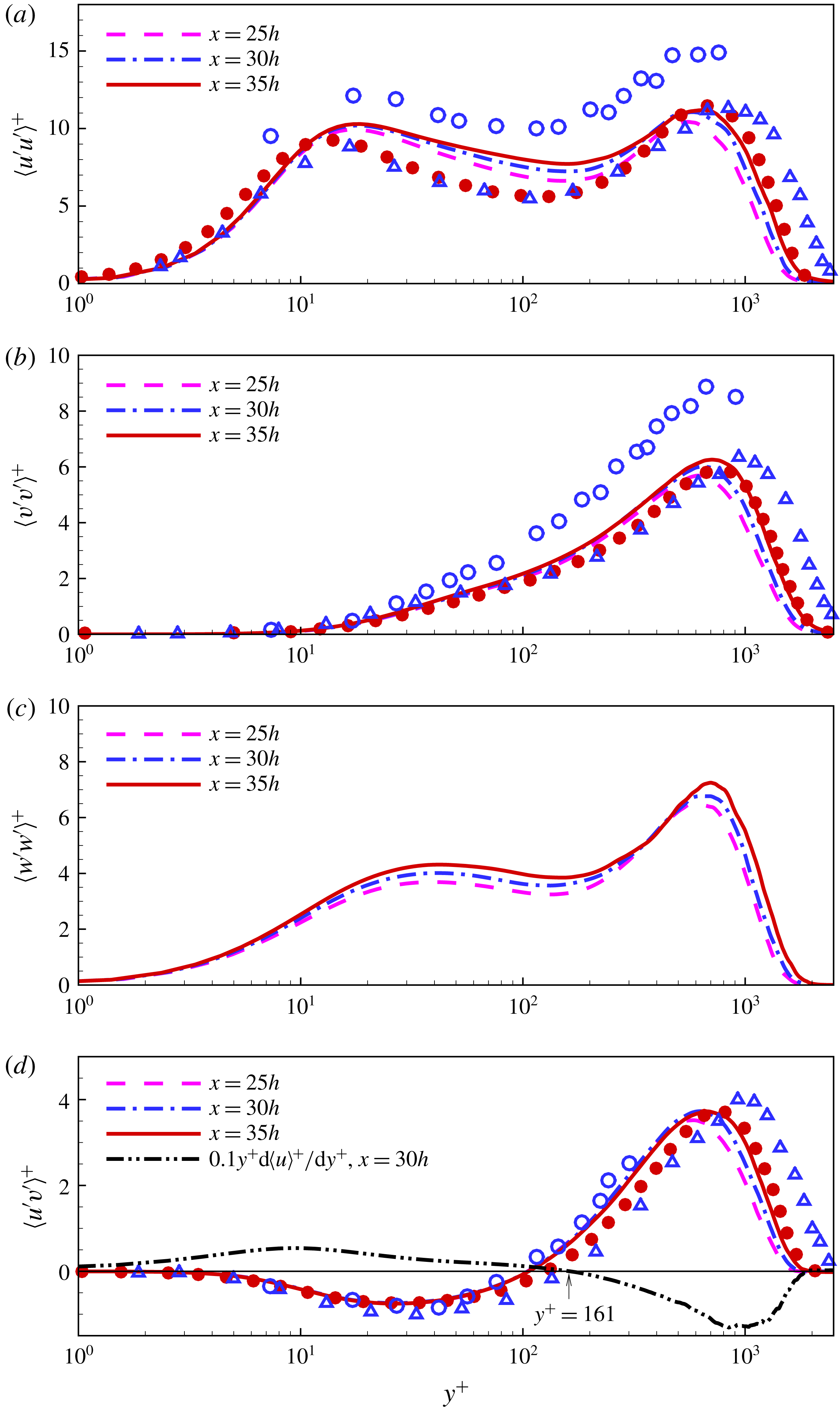
Figure 16. Inner-scaled Reynolds normal and shear stress profiles (a) streamwise
 $\langle u^{\prime }u^{\prime }\rangle ^{+}$
, (b) wall-normal
$\langle u^{\prime }u^{\prime }\rangle ^{+}$
, (b) wall-normal
 $\langle v^{\prime }v^{\prime }\rangle ^{+}$
, (c) spanwise
$\langle v^{\prime }v^{\prime }\rangle ^{+}$
, (c) spanwise
 $\langle w^{\prime }w^{\prime }\rangle ^{+}$
and (d) shear stress
$\langle w^{\prime }w^{\prime }\rangle ^{+}$
and (d) shear stress
 $\langle u^{\prime }v^{\prime }\rangle ^{+}$
and velocity gradient
$\langle u^{\prime }v^{\prime }\rangle ^{+}$
and velocity gradient
 $y^{+}(\text{d}\langle u\rangle ^{+}/\text{d}y^{+})$
at
$y^{+}(\text{d}\langle u\rangle ^{+}/\text{d}y^{+})$
at
 $x=30h$
. LES of Banyassady & Piomelli (Reference Banyassady and Piomelli2014) (●),
$x=30h$
. LES of Banyassady & Piomelli (Reference Banyassady and Piomelli2014) (●),
 $x=30h$
. Experimental data: Rostamy et al. (Reference Rostamy, Bergstrom, Sumner and Bugg2011a
) (○),
$x=30h$
. Experimental data: Rostamy et al. (Reference Rostamy, Bergstrom, Sumner and Bugg2011a
) (○),
 $x=30h$
; Eriksson et al. (Reference Eriksson, Karlsson and Persson1998) (▵),
$x=30h$
; Eriksson et al. (Reference Eriksson, Karlsson and Persson1998) (▵),
 $x=40h$
.
$x=40h$
.
Figure 16 shows the inner-scaled Reynolds normal and shear stress profiles. The friction velocity
 $u_{\unicode[STIX]{x1D70F}}$
and inner length scale
$u_{\unicode[STIX]{x1D70F}}$
and inner length scale
 $\unicode[STIX]{x1D708}/u_{\unicode[STIX]{x1D70F}}$
are the velocity and length scales. Again, the streamwise
$\unicode[STIX]{x1D708}/u_{\unicode[STIX]{x1D70F}}$
are the velocity and length scales. Again, the streamwise
 $\langle u^{\prime }u^{\prime }\rangle ^{+}$
, wall-normal
$\langle u^{\prime }u^{\prime }\rangle ^{+}$
, wall-normal
 $\langle v^{\prime }v^{\prime }\rangle ^{+}$
and shear stress
$\langle v^{\prime }v^{\prime }\rangle ^{+}$
and shear stress
 $\langle u^{\prime }v^{\prime }\rangle ^{+}$
profiles from the current DNS are compared with the experimental data of Eriksson et al. (Reference Eriksson, Karlsson and Persson1998) and Rostamy et al. (Reference Rostamy, Bergstrom, Sumner and Bugg2011a
) and the LES of Banyassady & Piomelli (Reference Banyassady and Piomelli2014). The measurements of Eriksson et al. (Reference Eriksson, Karlsson and Persson1998) and LES are close to the current DNS for
$\langle u^{\prime }v^{\prime }\rangle ^{+}$
profiles from the current DNS are compared with the experimental data of Eriksson et al. (Reference Eriksson, Karlsson and Persson1998) and Rostamy et al. (Reference Rostamy, Bergstrom, Sumner and Bugg2011a
) and the LES of Banyassady & Piomelli (Reference Banyassady and Piomelli2014). The measurements of Eriksson et al. (Reference Eriksson, Karlsson and Persson1998) and LES are close to the current DNS for
 $\langle v^{\prime }v^{\prime }\rangle ^{+}$
and
$\langle v^{\prime }v^{\prime }\rangle ^{+}$
and
 $\langle u^{\prime }v^{\prime }\rangle ^{+}$
and lower for
$\langle u^{\prime }v^{\prime }\rangle ^{+}$
and lower for
 $\langle u^{\prime }u^{\prime }\rangle ^{+}$
in the inner layer region. The inner layer region extends up to
$\langle u^{\prime }u^{\prime }\rangle ^{+}$
in the inner layer region. The inner layer region extends up to
 $y/y_{1/2}=0.2$
, or
$y/y_{1/2}=0.2$
, or
 $y^{+}=160$
. The measurements of Rostamy et al. (Reference Rostamy, Bergstrom, Sumner and Bugg2011a
) are significantly higher than the current DNS for
$y^{+}=160$
. The measurements of Rostamy et al. (Reference Rostamy, Bergstrom, Sumner and Bugg2011a
) are significantly higher than the current DNS for
 $\langle u^{\prime }u^{\prime }\rangle ^{+}$
and
$\langle u^{\prime }u^{\prime }\rangle ^{+}$
and
 $\langle v^{\prime }v^{\prime }\rangle ^{+}$
, whereas
$\langle v^{\prime }v^{\prime }\rangle ^{+}$
, whereas
 $\langle u^{\prime }v^{\prime }\rangle ^{+}$
is in agreement. The
$\langle u^{\prime }v^{\prime }\rangle ^{+}$
is in agreement. The
 $\langle v^{\prime }v^{\prime }\rangle ^{+}$
and
$\langle v^{\prime }v^{\prime }\rangle ^{+}$
and
 $\langle u^{\prime }v^{\prime }\rangle ^{+}$
profiles at
$\langle u^{\prime }v^{\prime }\rangle ^{+}$
profiles at
 $x/h=25$
, 30 and 35 collapse in the inner layer region. Whereas
$x/h=25$
, 30 and 35 collapse in the inner layer region. Whereas
 $\langle u^{\prime }u^{\prime }\rangle ^{+}$
and
$\langle u^{\prime }u^{\prime }\rangle ^{+}$
and
 $\langle w^{\prime }w^{\prime }\rangle ^{+}$
have a small variation, this is less than the uncertainty levels in the measurements (Rostamy et al.
Reference Rostamy, Bergstrom, Sumner and Bugg2011a
). Figure 16(d) also compares the velocity gradient profile
$\langle w^{\prime }w^{\prime }\rangle ^{+}$
have a small variation, this is less than the uncertainty levels in the measurements (Rostamy et al.
Reference Rostamy, Bergstrom, Sumner and Bugg2011a
). Figure 16(d) also compares the velocity gradient profile
 $y^{+}(\text{d}\langle u\rangle ^{+}/\text{d}y^{+})$
at
$y^{+}(\text{d}\langle u\rangle ^{+}/\text{d}y^{+})$
at
 $x=30h$
, with the Reynolds shear stress. The velocity gradient becomes zero at
$x=30h$
, with the Reynolds shear stress. The velocity gradient becomes zero at
 $y=y_{max}$
or
$y=y_{max}$
or
 $y^{+}=161$
, where the Reynolds shear stress has a finite positive value. Moreover, for a narrow region below
$y^{+}=161$
, where the Reynolds shear stress has a finite positive value. Moreover, for a narrow region below
 $y=y_{max}$
both the velocity gradient and Reynolds shear stress are positive. This invalidates the Boussinesq hypothesis
$y=y_{max}$
both the velocity gradient and Reynolds shear stress are positive. This invalidates the Boussinesq hypothesis
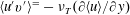 $\langle u^{\prime }v^{\prime }\rangle ^{=}-\unicode[STIX]{x1D708}_{T}(\unicode[STIX]{x2202}\langle u\rangle /\unicode[STIX]{x2202}y)$
for the wall jet, where the positive scalar coefficient
$\langle u^{\prime }v^{\prime }\rangle ^{=}-\unicode[STIX]{x1D708}_{T}(\unicode[STIX]{x2202}\langle u\rangle /\unicode[STIX]{x2202}y)$
for the wall jet, where the positive scalar coefficient
 $\unicode[STIX]{x1D708}_{T}$
is the turbulent viscosity. It also shows that the positive shear stress from the outer layer is transported against the velocity gradient below
$\unicode[STIX]{x1D708}_{T}$
is the turbulent viscosity. It also shows that the positive shear stress from the outer layer is transported against the velocity gradient below
 $y=y_{max}$
due to the turbulence transport.
$y=y_{max}$
due to the turbulence transport.
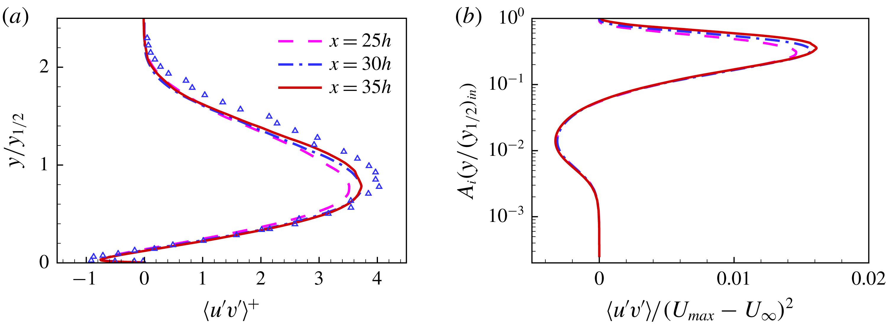
Figure 17. (a) Correct scaling of shear stress profile according to George et al. (Reference George, Abrahamsson, Eriksson, Karlsson, Lofdahal and Wosnik2000). Experimental data: Eriksson et al. (Reference Eriksson, Karlsson and Persson1998) (▵),
 $x=40h$
and (b) inner-scaled shear stress profiles with respect to incomplete similarity parameters (Barenblatt et al.
Reference Barenblatt, Chorin and Prostokishin2005).
$x=40h$
and (b) inner-scaled shear stress profiles with respect to incomplete similarity parameters (Barenblatt et al.
Reference Barenblatt, Chorin and Prostokishin2005).
George et al. (Reference George, Abrahamsson, Eriksson, Karlsson, Lofdahal and Wosnik2000) showed, using the asymptotic invariance principle (AIP), that for correct outer scaling, the shear stress
 $\langle u^{\prime }v^{\prime }\rangle$
should be normalized with the shear velocity
$\langle u^{\prime }v^{\prime }\rangle$
should be normalized with the shear velocity
 $u_{\unicode[STIX]{x1D70F}}^{2}$
. Figure 17(a) shows the shear stress profiles with this scaling. The profiles at
$u_{\unicode[STIX]{x1D70F}}^{2}$
. Figure 17(a) shows the shear stress profiles with this scaling. The profiles at
 $x/h=30$
and 35 show an improvement in their collapse with respect to this new scaling (George et al.
Reference George, Abrahamsson, Eriksson, Karlsson, Lofdahal and Wosnik2000) relative to the scaling based on a single velocity and length scale (Irwin Reference Irwin1973). This can be seen in figure 15(d). The current-scaled profiles are in agreement with the experimental data of Eriksson et al. (Reference Eriksson, Karlsson and Persson1998) up to
$x/h=30$
and 35 show an improvement in their collapse with respect to this new scaling (George et al.
Reference George, Abrahamsson, Eriksson, Karlsson, Lofdahal and Wosnik2000) relative to the scaling based on a single velocity and length scale (Irwin Reference Irwin1973). This can be seen in figure 15(d). The current-scaled profiles are in agreement with the experimental data of Eriksson et al. (Reference Eriksson, Karlsson and Persson1998) up to
 $y/y_{1/2}=0.8$
. Beyond this, experimental values for
$y/y_{1/2}=0.8$
. Beyond this, experimental values for
 $\langle u^{\prime }v^{\prime }\rangle ^{+}$
are higher. This might be due to the higher Reynolds number for the experiment and difference in wall friction velocity.
$\langle u^{\prime }v^{\prime }\rangle ^{+}$
are higher. This might be due to the higher Reynolds number for the experiment and difference in wall friction velocity.
Figure 17(b) shows the shear stress profiles scaled with incomplete similarity parameters (Barenblatt et al. Reference Barenblatt, Chorin and Prostokishin2005). It has been discussed earlier that the incomplete similarity parameters for the inner layer region would be consistent with the asymptotic invariance principle (George et al. Reference George, Abrahamsson, Eriksson, Karlsson, Lofdahal and Wosnik2000), if they scale the Reynolds shear stress. The figure shows a good collapse of shear stress profiles with this scaling in the inner layer region.

Figure 18. Frequency spectra of velocity and pressure fluctuations at
 $x/h=30$
(a) streamwise
$x/h=30$
(a) streamwise
 $E_{u^{\prime }}$
at:
$E_{u^{\prime }}$
at:
 $y^{+}=5$
(– – –);
$y^{+}=5$
(– – –);
 $y^{+}=17$
(— ⋅ —);
$y^{+}=17$
(— ⋅ —);
 $y/y_{1/2}=0.2$
(——);
$y/y_{1/2}=0.2$
(——);
 $y/y_{1/2}=0.8$
(— ⋅ ⋅ —), (b) wall-normal
$y/y_{1/2}=0.8$
(— ⋅ ⋅ —), (b) wall-normal
 $E_{v^{\prime }}$
at:
$E_{v^{\prime }}$
at:
 $y^{+}=5$
(– – –);
$y^{+}=5$
(– – –);
 $y^{+}=17$
(— ⋅ —);
$y^{+}=17$
(— ⋅ —);
 $y/y_{1/2}=0.2$
(——);
$y/y_{1/2}=0.2$
(——);
 $y_{1/2}=0.8$
(— ⋅ ⋅ —), (c) spanwise
$y_{1/2}=0.8$
(— ⋅ ⋅ —), (c) spanwise
 $E_{w^{\prime }}$
at:
$E_{w^{\prime }}$
at:
 $y^{+}=5$
(– – –);
$y^{+}=5$
(– – –);
 $y^{+}=40$
(— ⋅ —);
$y^{+}=40$
(— ⋅ —);
 $y/y_{1/2}=0.2$
(——);
$y/y_{1/2}=0.2$
(——);
 $y/y_{1/2}=0.8$
(— ⋅ ⋅ —) and (d) pressure
$y/y_{1/2}=0.8$
(— ⋅ ⋅ —) and (d) pressure
 $E_{p^{\prime }}$
at:
$E_{p^{\prime }}$
at:
 $y^{+}=5$
(– – –);
$y^{+}=5$
(– – –);
 $y^{+}=17$
(— ⋅ —);
$y^{+}=17$
(— ⋅ —);
 $y/y_{1/2}=0.2$
(——);
$y/y_{1/2}=0.2$
(——);
 $y/y_{1/2}=0.8$
(— ⋅ ⋅ —).
$y/y_{1/2}=0.8$
(— ⋅ ⋅ —).
The instantaneous values of velocity and pressure are saved at selected wall-normal locations at
 $x/h=30$
, for each time step from
$x/h=30$
, for each time step from
 $t^{\ast }=1200$
to 2500, giving 860 000 samples. Note,
$t^{\ast }=1200$
to 2500, giving 860 000 samples. Note,
 $St=fh/U_{j}$
is the Strouhal number or non-dimensional frequency and
$St=fh/U_{j}$
is the Strouhal number or non-dimensional frequency and
 $f$
is the frequency. As shown in figure 18, the streamwise
$f$
is the frequency. As shown in figure 18, the streamwise
 $E_{u^{\prime }}$
and wall-normal
$E_{u^{\prime }}$
and wall-normal
 $E_{v^{\prime }}$
spectra are given at
$E_{v^{\prime }}$
spectra are given at
 $y^{+}=5$
 $(y/y_{1/2}=0.006)$
,
$(y/y_{1/2}=0.006)$
,
 $y^{+}=17$
 $(y/y_{1/2}=0.02)$
,
$(y/y_{1/2}=0.02)$
,
 $y/y_{1/2}=0.2$
and
$y/y_{1/2}=0.2$
and
 $y/y_{1/2}=0.8$
. These locations represent the end of the linear region in the viscous sub layer, the first peak in
$y/y_{1/2}=0.8$
. These locations represent the end of the linear region in the viscous sub layer, the first peak in
 $\langle u^{\prime }u^{\prime }\rangle$
,
$\langle u^{\prime }u^{\prime }\rangle$
,
 $U_{max}$
and the outer layer peaks in
$U_{max}$
and the outer layer peaks in
 $\langle u^{\prime }u^{\prime }\rangle$
and
$\langle u^{\prime }u^{\prime }\rangle$
and
 $\langle v^{\prime }v^{\prime }\rangle$
, respectively. The Reynolds stress
$\langle v^{\prime }v^{\prime }\rangle$
, respectively. The Reynolds stress
 $\langle u^{\prime }u^{\prime }\rangle$
has a lower value at
$\langle u^{\prime }u^{\prime }\rangle$
has a lower value at
 $y^{+}=5$
, and contains less energy at the smaller scales relative to the other locations (figure 18
a). At the other three locations
$y^{+}=5$
, and contains less energy at the smaller scales relative to the other locations (figure 18
a). At the other three locations
 $\langle u^{\prime }u^{\prime }\rangle$
values are close to each other and so too are the spectra. The wall-normal Reynolds stress
$\langle u^{\prime }u^{\prime }\rangle$
values are close to each other and so too are the spectra. The wall-normal Reynolds stress
 $\langle v^{\prime }v^{\prime }\rangle$
increases continuously from the wall to a peak value around
$\langle v^{\prime }v^{\prime }\rangle$
increases continuously from the wall to a peak value around
 $y/y_{1/2}=0.8$
. Correspondingly spectra at increasing wall distance indicate a higher energy level. The spanwise velocity fluctuation spectra
$y/y_{1/2}=0.8$
. Correspondingly spectra at increasing wall distance indicate a higher energy level. The spanwise velocity fluctuation spectra
 $E_{w^{\prime }}$
(figure 18
c) are given at the same locations as
$E_{w^{\prime }}$
(figure 18
c) are given at the same locations as
 $E_{u^{\prime }}$
and
$E_{u^{\prime }}$
and
 $E_{v^{\prime }}$
, except for
$E_{v^{\prime }}$
, except for
 $y^{+}=40$
 $(y/y_{1/2}=0.05)$
, which is the first near wall peak in
$(y/y_{1/2}=0.05)$
, which is the first near wall peak in
 $\langle w^{\prime }w^{\prime }\rangle$
. The streamwise velocity fluctuation spectra show a
$\langle w^{\prime }w^{\prime }\rangle$
. The streamwise velocity fluctuation spectra show a
 $-5/3$
slope in the range of
$-5/3$
slope in the range of
 $0.06<St<2.0$
in the outer layer region. The wall-normal and spanwise velocity fluctuations spectra have a
$0.06<St<2.0$
in the outer layer region. The wall-normal and spanwise velocity fluctuations spectra have a
 $-5/3$
slope in a smaller range of frequencies
$-5/3$
slope in a smaller range of frequencies
 $0.4<St<2.0$
in the outer layer region. The higher frequency region is the viscous sub-range, where dissipation occurs and spectra can be compared to a line with a slope of
$0.4<St<2.0$
in the outer layer region. The higher frequency region is the viscous sub-range, where dissipation occurs and spectra can be compared to a line with a slope of
 $-7$
. The spectra in the inner layer region are closer to such a line as compared to the outer layer region.
$-7$
. The spectra in the inner layer region are closer to such a line as compared to the outer layer region.
In the low frequency region below
 $St<0.06$
spectra, particularly for
$St<0.06$
spectra, particularly for
 $E_{u^{\prime }}$
and
$E_{u^{\prime }}$
and
 $E_{v^{\prime }}$
, peaks indicating large scale fluctuations in the flow can be observed. Figure 18(d) shows the pressure spectra
$E_{v^{\prime }}$
, peaks indicating large scale fluctuations in the flow can be observed. Figure 18(d) shows the pressure spectra
 $E_{p^{\prime }}$
at identical locations to the spectra for
$E_{p^{\prime }}$
at identical locations to the spectra for
 $E_{u^{\prime }}$
and
$E_{u^{\prime }}$
and
 $E_{v^{\prime }}$
. The main features in the pressure spectra are multiple peaks in the low frequency range for
$E_{v^{\prime }}$
. The main features in the pressure spectra are multiple peaks in the low frequency range for
 $St<0.06$
, as observed for
$St<0.06$
, as observed for
 $E_{u^{\prime }}$
and
$E_{u^{\prime }}$
and
 $E_{v^{\prime }}$
. The peaks appear to be the signature of large scale structures passing in the outer layer region identified in figure 5.
$E_{v^{\prime }}$
. The peaks appear to be the signature of large scale structures passing in the outer layer region identified in figure 5.
3.4 Reynolds stresses and turbulence energy balance
An objective here is to present reliable turbulence kinetic energy
 $tke$
and Reynolds stresses budgets. The budgets are compared with a previously reported LES of Dejoan & Leschziner (Reference Dejoan and Leschziner2005). This LES is performed on a much coarser grid than the current DNS. The total number of LES grid points is more than an order of magnitude smaller than the DNS. The LES grid spacing, in streamwise and spanwise directions, is twice that of the current DNS. The dynamical equation for the Reynolds stress tensor in its non-dimensionalized form is given as
$tke$
and Reynolds stresses budgets. The budgets are compared with a previously reported LES of Dejoan & Leschziner (Reference Dejoan and Leschziner2005). This LES is performed on a much coarser grid than the current DNS. The total number of LES grid points is more than an order of magnitude smaller than the DNS. The LES grid spacing, in streamwise and spanwise directions, is twice that of the current DNS. The dynamical equation for the Reynolds stress tensor in its non-dimensionalized form is given as
 $$\begin{eqnarray}\displaystyle {\mathcal{C}}_{\langle u_{i}^{\prime }u_{j}^{\prime }\rangle }={\mathcal{P}}_{\langle u_{i}^{\prime }u_{j}^{\prime }\rangle }+\unicode[STIX]{x1D700}_{\langle u_{i}^{\prime }u_{j}^{\prime }\rangle }+{\mathcal{T}}_{\langle u_{i}^{\prime }u_{j}^{\prime }\rangle }+\unicode[STIX]{x1D6F9}_{\langle u_{i}^{\prime }u_{j}^{\prime }\rangle }+{\mathcal{D}}_{\langle u_{i}^{\prime }u_{j}^{\prime }\rangle }, & & \displaystyle\end{eqnarray}$$
where the following terms appear in this equation, with summation on repeated indices,
 $$\begin{eqnarray}\displaystyle & \displaystyle {\mathcal{C}}_{\langle u_{i}^{\prime }u_{j}^{\prime }\rangle }=\langle u_{k}\rangle \frac{\unicode[STIX]{x2202}\langle u_{i}^{\prime }u_{j}^{\prime }\rangle }{\unicode[STIX]{x2202}x_{k}}\quad \text{Convection}, & \displaystyle\end{eqnarray}$$
 $$\begin{eqnarray}\displaystyle & \displaystyle {\mathcal{P}}_{\langle u_{i}^{\prime }u_{j}^{\prime }\rangle }=-\langle u_{j}^{\prime }u_{k}^{\prime }\rangle \frac{\unicode[STIX]{x2202}\langle u_{i}\rangle }{\unicode[STIX]{x2202}x_{k}}-\langle u_{i}^{\prime }u_{k}^{\prime }\rangle \frac{\unicode[STIX]{x2202}\langle u_{j}\rangle }{\unicode[STIX]{x2202}x_{k}}\quad \text{Production}, & \displaystyle\end{eqnarray}$$
 $$\begin{eqnarray}\displaystyle & \displaystyle \unicode[STIX]{x1D700}_{\langle u_{i}^{\prime }u_{j}^{\prime }\rangle }=-\frac{2}{Re}\left\langle \left(\frac{\unicode[STIX]{x2202}u_{i}^{\prime }}{\unicode[STIX]{x2202}x_{k}}\right)\left(\frac{\unicode[STIX]{x2202}u_{j}^{\prime }}{\unicode[STIX]{x2202}x_{k}}\right)\right\rangle \quad \text{Dissipation}, & \displaystyle\end{eqnarray}$$
 $$\begin{eqnarray}\displaystyle & \displaystyle {\mathcal{T}}_{\langle u_{i}^{\prime }u_{j}^{\prime }\rangle }=-\frac{\unicode[STIX]{x2202}\langle u_{i}^{\prime }u_{j}^{\prime }u_{k}^{\prime }\rangle }{\unicode[STIX]{x2202}x_{k}}\quad \text{Turbulent diffusion}, & \displaystyle\end{eqnarray}$$
 $$\begin{eqnarray}\displaystyle & \displaystyle \unicode[STIX]{x1D6F9}_{\langle u_{i}^{\prime }u_{j}^{\prime }\rangle }=-\left\langle u_{j}^{\prime }\frac{\unicode[STIX]{x2202}p^{\prime }}{\unicode[STIX]{x2202}x_{i}}\right\rangle -\left\langle u_{i}^{\prime }\frac{\unicode[STIX]{x2202}p^{\prime }}{\unicode[STIX]{x2202}x_{j}}\right\rangle \quad \text{Velocity{-}pressure gradient correlation}, & \displaystyle\end{eqnarray}$$
 $$\begin{eqnarray}\displaystyle & \displaystyle {\mathcal{D}}_{\langle u_{i}^{\prime }u_{j}^{\prime }\rangle }=\frac{1}{Re}\frac{\unicode[STIX]{x2202}^{2}\langle u_{i}^{\prime }u_{j}^{\prime }\rangle }{\unicode[STIX]{x2202}x_{k}\unicode[STIX]{x2202}x_{k}}\quad \text{Viscous diffusion}. & \displaystyle\end{eqnarray}$$
Note,
 $tke=(1/2)(\langle u^{\prime }u^{\prime }\rangle +\langle v^{\prime }v^{\prime }\rangle +\langle w^{\prime }w^{\prime }\rangle )$
, and its budget can be calculated by summing the budgets of individual Reynolds normal stresses given by (3.15).
$tke=(1/2)(\langle u^{\prime }u^{\prime }\rangle +\langle v^{\prime }v^{\prime }\rangle +\langle w^{\prime }w^{\prime }\rangle )$
, and its budget can be calculated by summing the budgets of individual Reynolds normal stresses given by (3.15).

Figure 19. Turbulence kinetic energy (
 $tke$
), Reynolds normal and shear stress budgets in the near wall region. The terms are normalized with
$tke$
), Reynolds normal and shear stress budgets in the near wall region. The terms are normalized with
 $u_{\unicode[STIX]{x1D70F}}^{4}/\unicode[STIX]{x1D708}$
: (a)
$u_{\unicode[STIX]{x1D70F}}^{4}/\unicode[STIX]{x1D708}$
: (a)
 $tke=(\langle u^{\prime }u^{\prime }\rangle +\langle v^{\prime }v^{\prime }\rangle +\langle w^{\prime }w^{\prime }\rangle )/2$
; (b)
$tke=(\langle u^{\prime }u^{\prime }\rangle +\langle v^{\prime }v^{\prime }\rangle +\langle w^{\prime }w^{\prime }\rangle )/2$
; (b)
 $\langle u^{\prime }u^{\prime }\rangle$
; (c)
$\langle u^{\prime }u^{\prime }\rangle$
; (c)
 $\langle v^{\prime }v^{\prime }\rangle$
; (d)
$\langle v^{\prime }v^{\prime }\rangle$
; (d)
 $\langle w^{\prime }w^{\prime }\rangle$
and (e)
$\langle w^{\prime }w^{\prime }\rangle$
and (e)
 $\langle u^{\prime }v^{\prime }\rangle$
. LES of wall jet by Dejoan & Leschziner (Reference Dejoan and Leschziner2005): production (▴); dissipation (▪); velocity–pressure gradient correlation (●); turbulent diffusion (▾). DNS of turbulent boundary layer by Spalart (Reference Spalart1988): production (▵); dissipation (▫); velocity–pressure gradient correlation (○); turbulent diffusion (▿).
$\langle u^{\prime }v^{\prime }\rangle$
. LES of wall jet by Dejoan & Leschziner (Reference Dejoan and Leschziner2005): production (▴); dissipation (▪); velocity–pressure gradient correlation (●); turbulent diffusion (▾). DNS of turbulent boundary layer by Spalart (Reference Spalart1988): production (▵); dissipation (▫); velocity–pressure gradient correlation (○); turbulent diffusion (▿).
3.4.1 Inner-scaled budgets
Figure 19 shows the budgets for
 $tke$
, Reynolds normal and shear stresses at
$tke$
, Reynolds normal and shear stresses at
 $x/h=30$
in the inner layer region. The profiles are scaled with the inner variables, whereas the budget terms are normalized with
$x/h=30$
in the inner layer region. The profiles are scaled with the inner variables, whereas the budget terms are normalized with
 $u_{\unicode[STIX]{x1D70F}}^{4}/\unicode[STIX]{x1D708}$
. The balance or the sum of all the budget terms for each Reynolds stress is
$u_{\unicode[STIX]{x1D70F}}^{4}/\unicode[STIX]{x1D708}$
. The balance or the sum of all the budget terms for each Reynolds stress is
 $O(10^{-2})$
of the maximum value. As mentioned earlier, the current budgets are compared with the wall jet LES of Dejoan & Leschziner (Reference Dejoan and Leschziner2005). This LES might be the only published budget for comparison for wall jets in the inner layer region. The LES based budget is given at
$O(10^{-2})$
of the maximum value. As mentioned earlier, the current budgets are compared with the wall jet LES of Dejoan & Leschziner (Reference Dejoan and Leschziner2005). This LES might be the only published budget for comparison for wall jets in the inner layer region. The LES based budget is given at
 $x/h=20$
and only the dominant terms from that budget are included here. The dominant terms of the turbulence kinetic energy and Reynolds stress budgets from the flat plate turbulent boundary layer DNS of Spalart (Reference Spalart1988) are also included in figure 19. This helps to understand how closely the inner layer of the plane wall jet follows a turbulent boundary layer flow.
$x/h=20$
and only the dominant terms from that budget are included here. The dominant terms of the turbulence kinetic energy and Reynolds stress budgets from the flat plate turbulent boundary layer DNS of Spalart (Reference Spalart1988) are also included in figure 19. This helps to understand how closely the inner layer of the plane wall jet follows a turbulent boundary layer flow.
It is clearly shown that (figure 19 a,b,d,e) the dominant terms of production, dissipation and velocity–pressure gradient correlation for turbulent kinetic energy, Reynolds streamwise, spanwise and shear stress budgets for the wall jet and boundary layer are in agreement. The wall-normal Reynolds stress budget shows (figure 19 c) that the dominant terms of dissipation and velocity–pressure gradient correlation have different peak values from the boundary layer, however the trend is the same for both flows. The turbulent transport term for the wall-normal and shear stress budgets indicate a major deviation of the wall jet from the turbulent boundary layer. This has a significant effect on the Reynolds wall-normal and shear stress distribution of the wall jet.
In figure 19(a) a comparison of the
 $tke$
budget with previously reported LES (Dejoan & Leschziner Reference Dejoan and Leschziner2005) shows that the level of production is lower than the current DNS and the trend for the dissipation does not match below
$tke$
budget with previously reported LES (Dejoan & Leschziner Reference Dejoan and Leschziner2005) shows that the level of production is lower than the current DNS and the trend for the dissipation does not match below
 $y^{+}=20$
. The Reynolds wall-normal and shear stress budgets (figure 19
c,e) from LES show even more drastic deviation from the current DNS. In the case of Reynolds shear stress the LES gives a significantly lower level of production and velocity–pressure gradient correlation. The wall-normal stress from the LES does not follow standard wall behaviour, rather than velocity–pressure gradient correlation term it gives turbulent transport as the dominant term, which is balanced by the dissipation. Moreover, the trend for turbulent transport and level of dissipation for wall-normal stress from LES do not match with the current DNS. A possible explanation is that the LES predicted these budgets at
$y^{+}=20$
. The Reynolds wall-normal and shear stress budgets (figure 19
c,e) from LES show even more drastic deviation from the current DNS. In the case of Reynolds shear stress the LES gives a significantly lower level of production and velocity–pressure gradient correlation. The wall-normal stress from the LES does not follow standard wall behaviour, rather than velocity–pressure gradient correlation term it gives turbulent transport as the dominant term, which is balanced by the dissipation. Moreover, the trend for turbulent transport and level of dissipation for wall-normal stress from LES do not match with the current DNS. A possible explanation is that the LES predicted these budgets at
 $x/h=20$
, where the wall jet boundary layer may not be fully developed and the outer shear layer is interacting with the wall. However, the current DNS shows that the velocity–pressure gradient term is dominant for the
$x/h=20$
, where the wall jet boundary layer may not be fully developed and the outer shear layer is interacting with the wall. However, the current DNS shows that the velocity–pressure gradient term is dominant for the
 $\langle v^{\prime }v^{\prime }\rangle$
budget in the inner layer region as far upstream as
$\langle v^{\prime }v^{\prime }\rangle$
budget in the inner layer region as far upstream as
 $x/h=15$
. Also, the dissipation term in the LES is not calculated explicitly, but evaluated as a balance from the rest of the terms. This might be responsible for the near wall difference below
$x/h=15$
. Also, the dissipation term in the LES is not calculated explicitly, but evaluated as a balance from the rest of the terms. This might be responsible for the near wall difference below
 $y^{+}=20$
in
$y^{+}=20$
in
 $\langle u^{\prime }u^{\prime }\rangle$
, where sub-grid modelling may have some deficiencies. The overall difference between the current DNS and LES is due to the lower grid resolution of the latter, as mentioned earlier.
$\langle u^{\prime }u^{\prime }\rangle$
, where sub-grid modelling may have some deficiencies. The overall difference between the current DNS and LES is due to the lower grid resolution of the latter, as mentioned earlier.
For the DNS, as can be seen from figure 19(a) in the inner layer region, the turbulent kinetic energy budget shows that the dissipation is balanced by viscous diffusion in the viscous sub-layer for
 $y^{+}<5$
. The production term has high values outside the viscous sub-layer in the range of
$y^{+}<5$
. The production term has high values outside the viscous sub-layer in the range of
 $5\leqslant y^{+}\leqslant 50$
, with a peak around
$5\leqslant y^{+}\leqslant 50$
, with a peak around
 $y^{+}=12$
. This high value of production is balanced mainly by dissipation and up to a certain extent, by turbulence diffusion. Eriksson (Reference Eriksson2003) estimated the near wall dissipation value as 0.27, which is 12 % lower than the current value of 0.31.
$y^{+}=12$
. This high value of production is balanced mainly by dissipation and up to a certain extent, by turbulence diffusion. Eriksson (Reference Eriksson2003) estimated the near wall dissipation value as 0.27, which is 12 % lower than the current value of 0.31.
Figure 19(b) shows the streamwise Reynolds stress
 $\langle u^{\prime }u^{\prime }\rangle$
budget. This is similar to the turbulence kinetic energy budget, except for the velocity–pressure gradient correlation term. This changes the sign and balances production along with dissipation and turbulent diffusion. The velocity–pressure gradient correlation transfers streamwise energy to other directions. The high level of production in the region of
$\langle u^{\prime }u^{\prime }\rangle$
budget. This is similar to the turbulence kinetic energy budget, except for the velocity–pressure gradient correlation term. This changes the sign and balances production along with dissipation and turbulent diffusion. The velocity–pressure gradient correlation transfers streamwise energy to other directions. The high level of production in the region of
 $5\leqslant y^{+}\leqslant 50$
is responsible for the inner layer peak of the streamwise Reynolds stress (figure 16
a). For the wall-normal stress
$5\leqslant y^{+}\leqslant 50$
is responsible for the inner layer peak of the streamwise Reynolds stress (figure 16
a). For the wall-normal stress
 $\langle v^{\prime }v^{\prime }\rangle$
budget in the inner layer region (figure 19
c), the dissipation is mainly balanced with the velocity–pressure gradient correlation and turbulent diffusion terms. The production is small and wall-normal turbulence in the inner layer region is maintained by turbulent diffusion and velocity–pressure gradient correlation. These transfer turbulence energy from the streamwise to the wall-normal direction. Figure 19(d) shows the budget for the spanwise Reynolds stress
$\langle v^{\prime }v^{\prime }\rangle$
budget in the inner layer region (figure 19
c), the dissipation is mainly balanced with the velocity–pressure gradient correlation and turbulent diffusion terms. The production is small and wall-normal turbulence in the inner layer region is maintained by turbulent diffusion and velocity–pressure gradient correlation. These transfer turbulence energy from the streamwise to the wall-normal direction. Figure 19(d) shows the budget for the spanwise Reynolds stress
 $\langle w^{\prime }w^{\prime }\rangle$
. The dissipation is balanced by viscous diffusion in the viscous sub-layer region
$\langle w^{\prime }w^{\prime }\rangle$
. The dissipation is balanced by viscous diffusion in the viscous sub-layer region
 $y^{+}<5$
. Outside the viscous sub-layer, it is balanced with the velocity–pressure gradient term. The Reynolds shear stress
$y^{+}<5$
. Outside the viscous sub-layer, it is balanced with the velocity–pressure gradient term. The Reynolds shear stress
 $\langle u^{\prime }v^{\prime }\rangle$
budget (figure 19
e) has high negative production, which is balanced by the velocity–pressure gradient term and turbulent diffusion.
$\langle u^{\prime }v^{\prime }\rangle$
budget (figure 19
e) has high negative production, which is balanced by the velocity–pressure gradient term and turbulent diffusion.

Figure 20. Turbulence kinetic energy (
 $tke$
), Reynolds normal and shear stress budgets in the outer layer region. The terms are normalized with
$tke$
), Reynolds normal and shear stress budgets in the outer layer region. The terms are normalized with
 $(U_{max}-U_{\infty })^{3}/y_{1/2}$
. Legends for DNS are same as in figure 19. (a)
$(U_{max}-U_{\infty })^{3}/y_{1/2}$
. Legends for DNS are same as in figure 19. (a)
 $tke=(\langle u^{\prime }u^{\prime }\rangle +\langle v^{\prime }v^{\prime }\rangle +\langle w^{\prime }w^{\prime }\rangle )/2$
, (b)
$tke=(\langle u^{\prime }u^{\prime }\rangle +\langle v^{\prime }v^{\prime }\rangle +\langle w^{\prime }w^{\prime }\rangle )/2$
, (b)
 $\langle u^{\prime }u^{\prime }\rangle$
, (c)
$\langle u^{\prime }u^{\prime }\rangle$
, (c)
 $\langle v^{\prime }v^{\prime }\rangle$
, (d)
$\langle v^{\prime }v^{\prime }\rangle$
, (d)
 $\langle w^{\prime }w^{\prime }\rangle$
and (e)
$\langle w^{\prime }w^{\prime }\rangle$
and (e)
 $\langle u^{\prime }v^{\prime }\rangle$
. LES of wall jet by Dejoan & Leschziner (Reference Dejoan and Leschziner2005): production (▴); dissipation (▪); velocity–pressure gradient correlation (●). Experimental data, Irwin (Reference Irwin1973): production (▵); dissipation (▫); turbulent diffusion (
$\langle u^{\prime }v^{\prime }\rangle$
. LES of wall jet by Dejoan & Leschziner (Reference Dejoan and Leschziner2005): production (▴); dissipation (▪); velocity–pressure gradient correlation (●). Experimental data, Irwin (Reference Irwin1973): production (▵); dissipation (▫); turbulent diffusion (
 $+$
) and Zhou et al. (Reference Zhou, Heine and Wygnanski1996): Production (▿); dissipation (♢); turbulent diffusion (
$+$
) and Zhou et al. (Reference Zhou, Heine and Wygnanski1996): Production (▿); dissipation (♢); turbulent diffusion (
 $\ast$
).
$\ast$
).
3.4.2 Outer-scaled budgets
Figure 20 shows the turbulence kinetic energy, Reynolds normal and shear stress budgets at
 $x/h=30$
in the outer layer region. The budget terms are normalized with
$x/h=30$
in the outer layer region. The budget terms are normalized with
 $(U_{max}-U_{\infty })^{3}$
and wall-normal distance with
$(U_{max}-U_{\infty })^{3}$
and wall-normal distance with
 $y_{1/2}$
. The balance for the outer-scaled budgets is less than 4 % of the peak values of production and dissipation. The outer scale LES budgets of Dejoan & Leschziner (Reference Dejoan and Leschziner2005) are compared with the current DNS. The predicted turbulence kinetic energy budget is also compared with the measurements of Irwin (Reference Irwin1973) and Zhou et al. (Reference Zhou, Heine and Wygnanski1996).
$y_{1/2}$
. The balance for the outer-scaled budgets is less than 4 % of the peak values of production and dissipation. The outer scale LES budgets of Dejoan & Leschziner (Reference Dejoan and Leschziner2005) are compared with the current DNS. The predicted turbulence kinetic energy budget is also compared with the measurements of Irwin (Reference Irwin1973) and Zhou et al. (Reference Zhou, Heine and Wygnanski1996).
Figure 20(a) shows the outer-scaled turbulent kinetic energy budget, where all the terms have been evaluated explicitly for the current DNS. The viscous diffusion and velocity–pressure gradient terms are negligible in the outer layer region. The production and convection terms are mainly balanced by turbulent diffusion and dissipation. The production term has a minimum around
 $y_{max}$
, however it always remains positive. The production, dissipation and turbulent transport terms are compared with the measurements. In the experiments only turbulent transport can be measured directly and the DNS values lie between the two sets of measurements (Irwin Reference Irwin1973; Zhou et al.
Reference Zhou, Heine and Wygnanski1996) and is closer to Irwin’s data. In experiments the production is estimated from a mean curve drawn through the measured mean velocity values (Irwin Reference Irwin1973). Both experiments cited here give identical values of production and are close to the current DNS. The dissipation is estimated either from local spectra using the
$y_{max}$
, however it always remains positive. The production, dissipation and turbulent transport terms are compared with the measurements. In the experiments only turbulent transport can be measured directly and the DNS values lie between the two sets of measurements (Irwin Reference Irwin1973; Zhou et al.
Reference Zhou, Heine and Wygnanski1996) and is closer to Irwin’s data. In experiments the production is estimated from a mean curve drawn through the measured mean velocity values (Irwin Reference Irwin1973). Both experiments cited here give identical values of production and are close to the current DNS. The dissipation is estimated either from local spectra using the
 $-5/3$
law (Irwin Reference Irwin1973) or using the assumption of local isotropy along with Taylor’s hypothesis (Zhou et al.
Reference Zhou, Heine and Wygnanski1996). The dissipation estimates from Irwin (Reference Irwin1973) are close to the current DNS, whereas Zhou et al. (Reference Zhou, Heine and Wygnanski1996) have estimated a higher level of dissipation. The current DNS shows that the assumption of isotropy in dissipation is not valid in the inner layer region below
$-5/3$
law (Irwin Reference Irwin1973) or using the assumption of local isotropy along with Taylor’s hypothesis (Zhou et al.
Reference Zhou, Heine and Wygnanski1996). The dissipation estimates from Irwin (Reference Irwin1973) are close to the current DNS, whereas Zhou et al. (Reference Zhou, Heine and Wygnanski1996) have estimated a higher level of dissipation. The current DNS shows that the assumption of isotropy in dissipation is not valid in the inner layer region below
 $y/y_{1/2}=0.2=y_{max}$
. The DNS shows that in the outer layer region for
$y/y_{1/2}=0.2=y_{max}$
. The DNS shows that in the outer layer region for
 $0.2\leqslant y/y_{1/2}\leqslant 1$
the wall-normal dissipation
$0.2\leqslant y/y_{1/2}\leqslant 1$
the wall-normal dissipation
 $\langle (\unicode[STIX]{x2202}v^{\prime }/\unicode[STIX]{x2202}x_{k})(\unicode[STIX]{x2202}v^{\prime }/\unicode[STIX]{x2202}x_{k})\rangle$
is 15–20 % smaller and the spanwise dissipation
$\langle (\unicode[STIX]{x2202}v^{\prime }/\unicode[STIX]{x2202}x_{k})(\unicode[STIX]{x2202}v^{\prime }/\unicode[STIX]{x2202}x_{k})\rangle$
is 15–20 % smaller and the spanwise dissipation
 $\langle (\unicode[STIX]{x2202}w^{\prime }/\unicode[STIX]{x2202}x_{k})(\unicode[STIX]{x2202}w^{\prime }/\unicode[STIX]{x2202}x_{k})\rangle$
is 10–15 % smaller than the streamwise dissipation
$\langle (\unicode[STIX]{x2202}w^{\prime }/\unicode[STIX]{x2202}x_{k})(\unicode[STIX]{x2202}w^{\prime }/\unicode[STIX]{x2202}x_{k})\rangle$
is 10–15 % smaller than the streamwise dissipation
 $\langle (\unicode[STIX]{x2202}u^{\prime }/\unicode[STIX]{x2202}x_{k})(\unicode[STIX]{x2202}u^{\prime }/\unicode[STIX]{x2202}x_{k})\rangle$
, respectively. The dominant terms of production and velocity–pressure gradient correlation from LES (Dejoan & Leschziner Reference Dejoan and Leschziner2005) are slightly lower than the current DNS, whereas the dissipation is in good agreement for various budgets.
$\langle (\unicode[STIX]{x2202}u^{\prime }/\unicode[STIX]{x2202}x_{k})(\unicode[STIX]{x2202}u^{\prime }/\unicode[STIX]{x2202}x_{k})\rangle$
, respectively. The dominant terms of production and velocity–pressure gradient correlation from LES (Dejoan & Leschziner Reference Dejoan and Leschziner2005) are slightly lower than the current DNS, whereas the dissipation is in good agreement for various budgets.
Figure 20(b) shows the outer-scaled streamwise Reynolds stress
 $\langle u^{\prime }u^{\prime }\rangle$
budget. The production has high positive values in the range of
$\langle u^{\prime }u^{\prime }\rangle$
budget. The production has high positive values in the range of
 $0.2<y/y_{1/2}<1.5$
, which is responsible for high values of Reynolds stress
$0.2<y/y_{1/2}<1.5$
, which is responsible for high values of Reynolds stress
 $\langle u^{\prime }u^{\prime }\rangle$
in the outer layer region. A portion of this energy is dissipated and the remainder transfers to turbulent and velocity–pressure gradient diffusion. The turbulent production has a minimum value at
$\langle u^{\prime }u^{\prime }\rangle$
in the outer layer region. A portion of this energy is dissipated and the remainder transfers to turbulent and velocity–pressure gradient diffusion. The turbulent production has a minimum value at
 $y_{max}$
, where maximum mean velocity occurs and
$y_{max}$
, where maximum mean velocity occurs and
 $\unicode[STIX]{x2202}\langle u\rangle /\unicode[STIX]{x2202}y=0$
. At this location, turbulence is maintained by the turbulent diffusion term. This transports the turbulence energy from the outer high energy region. The velocity–pressure gradient diffusion term transfers energy from the streamwise direction to the wall-normal and spanwise turbulence components. The wall-normal Reynolds stress
$\unicode[STIX]{x2202}\langle u\rangle /\unicode[STIX]{x2202}y=0$
. At this location, turbulence is maintained by the turbulent diffusion term. This transports the turbulence energy from the outer high energy region. The velocity–pressure gradient diffusion term transfers energy from the streamwise direction to the wall-normal and spanwise turbulence components. The wall-normal Reynolds stress
 $\langle v^{\prime }v^{\prime }\rangle$
has little production in the outer layer region (figure 20
c). The turbulence is mainly driven by the velocity–pressure gradient correlation term, which is balanced by the dissipation and turbulent diffusion terms. The spanwise Reynolds stress
$\langle v^{\prime }v^{\prime }\rangle$
has little production in the outer layer region (figure 20
c). The turbulence is mainly driven by the velocity–pressure gradient correlation term, which is balanced by the dissipation and turbulent diffusion terms. The spanwise Reynolds stress
 $\langle w^{\prime }w^{\prime }\rangle$
budget shows that the velocity–pressure gradient and convection terms are balanced with the dissipation and turbulent diffusion terms in the outer layer region (figure 20
d). The turbulent diffusion term transfers energy from the outer layer region to the inner layer maintaining turbulence around
$\langle w^{\prime }w^{\prime }\rangle$
budget shows that the velocity–pressure gradient and convection terms are balanced with the dissipation and turbulent diffusion terms in the outer layer region (figure 20
d). The turbulent diffusion term transfers energy from the outer layer region to the inner layer maintaining turbulence around
 $y_{max}$
.
$y_{max}$
.
The shear stress budget
 $\langle u^{\prime }v^{\prime }\rangle$
has the production and velocity–pressure gradient as the dominant terms, which balance each other (figure 20
e). In the outer layer region, production is positive and is responsible for high values of shear stress
$\langle u^{\prime }v^{\prime }\rangle$
has the production and velocity–pressure gradient as the dominant terms, which balance each other (figure 20
e). In the outer layer region, production is positive and is responsible for high values of shear stress
 $\langle u^{\prime }v^{\prime }\rangle$
. At
$\langle u^{\prime }v^{\prime }\rangle$
. At
 $y=y_{max}$
the velocity gradient and production become zero and below this point production is negative, however shear stress remains positive for some distance in this region. The turbulent diffusion is responsible for a positive shear stress at and below
$y=y_{max}$
the velocity gradient and production become zero and below this point production is negative, however shear stress remains positive for some distance in this region. The turbulent diffusion is responsible for a positive shear stress at and below
 $y=y_{max}$
, where production is zero or negative.
$y=y_{max}$
, where production is zero or negative.

Figure 21. The inner-scaled velocity–pressure gradient correlation, pressure diffusion and pressure–strain correlation profiles in the near wall region for: (a)
 $tke=(\langle u^{\prime }u^{\prime }\rangle +\langle v^{\prime }v^{\prime }\rangle +\langle w^{\prime }w^{\prime }\rangle )/2$
; (b)
$tke=(\langle u^{\prime }u^{\prime }\rangle +\langle v^{\prime }v^{\prime }\rangle +\langle w^{\prime }w^{\prime }\rangle )/2$
; (b)
 $\langle u^{\prime }u^{\prime }\rangle$
; (c)
$\langle u^{\prime }u^{\prime }\rangle$
; (c)
 $\langle v^{\prime }v^{\prime }\rangle$
; (d)
$\langle v^{\prime }v^{\prime }\rangle$
; (d)
 $\langle v^{\prime }v^{\prime }\rangle$
channel flow (Mansour, Kim & Moin Reference Mansour, Kim and Moin1988); (e)
$\langle v^{\prime }v^{\prime }\rangle$
channel flow (Mansour, Kim & Moin Reference Mansour, Kim and Moin1988); (e)
 $\langle w^{\prime }w^{\prime }\rangle$
and (f)
$\langle w^{\prime }w^{\prime }\rangle$
and (f)
 $\langle u^{\prime }v^{\prime }\rangle$
.
$\langle u^{\prime }v^{\prime }\rangle$
.
3.4.3 Velocity–pressure gradient and triple-velocity correlations
It has been shown from the budgets that for the wall jet, velocity–pressure gradient correlation and turbulent transport terms show the influence of the outer layer and depart from pure boundary layer behaviour. The velocity–pressure gradient correlation is responsible for energy redistribution among various Reynolds stresses. This term can be split as
 $$\begin{eqnarray}\displaystyle \unicode[STIX]{x1D6F9}_{\langle u_{i}^{\prime }u_{j}^{\prime }\rangle }=-\left\langle \frac{\unicode[STIX]{x2202}p^{\prime }u_{j}^{\prime }}{\unicode[STIX]{x2202}x_{i}}+\frac{\unicode[STIX]{x2202}p^{\prime }u_{i}^{\prime }}{\unicode[STIX]{x2202}x_{j}}\right\rangle +\unicode[STIX]{x1D719}_{ij} & & \displaystyle\end{eqnarray}$$
and
 $$\begin{eqnarray}\displaystyle \unicode[STIX]{x1D719}_{ij}=\left\langle p^{\prime }\left(\frac{\unicode[STIX]{x2202}u_{j}^{\prime }}{\unicode[STIX]{x2202}x_{i}}+\frac{\unicode[STIX]{x2202}u_{i}^{\prime }}{\unicode[STIX]{x2202}x_{j}}\right)\right\rangle . & & \displaystyle\end{eqnarray}$$
The first term on the right-hand side in (3.22) is described as pressure diffusion or pressure transport and the second term
 $\unicode[STIX]{x1D719}_{ij}$
as pressure–strain correlation. The pressure strain term is the main redistributive component, which transfers energy from one component of turbulent kinetic energy to another. Negative values of pressure–strain correlation indicate loss and positive values indicate gain of energy by the corresponding Reynolds stress component. The trace of
$\unicode[STIX]{x1D719}_{ij}$
as pressure–strain correlation. The pressure strain term is the main redistributive component, which transfers energy from one component of turbulent kinetic energy to another. Negative values of pressure–strain correlation indicate loss and positive values indicate gain of energy by the corresponding Reynolds stress component. The trace of
 $\unicode[STIX]{x1D719}_{ij}$
is zero. Figure 21 shows the inner-scaled profiles for velocity–pressure gradient, pressure–strain and pressure diffusion term in the near wall region for turbulent kinetic energy, Reynolds normal and shear stresses. The terms
$\unicode[STIX]{x1D719}_{ij}$
is zero. Figure 21 shows the inner-scaled profiles for velocity–pressure gradient, pressure–strain and pressure diffusion term in the near wall region for turbulent kinetic energy, Reynolds normal and shear stresses. The terms
 $\unicode[STIX]{x1D6F9}_{\langle u_{i}^{\prime }u_{j}^{\prime }\rangle }$
,
$\unicode[STIX]{x1D6F9}_{\langle u_{i}^{\prime }u_{j}^{\prime }\rangle }$
,
 $\unicode[STIX]{x1D719}_{ij}$
and pressure diffusion for wall-normal Reynolds stress for a channel flow (Mansour et al.
Reference Mansour, Kim and Moin1988) are also included (figure 21
d) for comparison. It is important to note here that in the current DNS velocity–pressure gradient and pressure–strain correlations are calculated explicitly and pressure diffusion is the difference of the two terms.
$\unicode[STIX]{x1D719}_{ij}$
and pressure diffusion for wall-normal Reynolds stress for a channel flow (Mansour et al.
Reference Mansour, Kim and Moin1988) are also included (figure 21
d) for comparison. It is important to note here that in the current DNS velocity–pressure gradient and pressure–strain correlations are calculated explicitly and pressure diffusion is the difference of the two terms.
The pressure–strain for turbulent kinetic energy is zero (figure 21
a), which is the trace of
 $\unicode[STIX]{x1D719}_{ij}$
. It shows that the explicitly calculated pressure–strain is following the expected behaviour. In case of streamwise fluctuations the velocity–pressure gradient mainly consists of the pressure–strain correlation (figure 21
b), which is negative, indicating energy transfer from the streamwise to other directions.
$\unicode[STIX]{x1D719}_{ij}$
. It shows that the explicitly calculated pressure–strain is following the expected behaviour. In case of streamwise fluctuations the velocity–pressure gradient mainly consists of the pressure–strain correlation (figure 21
b), which is negative, indicating energy transfer from the streamwise to other directions.
The
 $\unicode[STIX]{x1D6F9}_{\langle u_{i}^{\prime }u_{j}^{\prime }\rangle }$
and
$\unicode[STIX]{x1D6F9}_{\langle u_{i}^{\prime }u_{j}^{\prime }\rangle }$
and
 $\unicode[STIX]{x1D719}_{ij}$
show more interesting behaviour for the Reynolds wall-normal and shear stresses. It has been shown for wall turbulence, e.g. in channel flow (figure 21
d) (Mansour et al.
Reference Mansour, Kim and Moin1988), that for wall-normal Reynolds stress, velocity–pressure gradient and pressure–strain correlation follow the same trend and values, except very close to surface below
$\unicode[STIX]{x1D719}_{ij}$
show more interesting behaviour for the Reynolds wall-normal and shear stresses. It has been shown for wall turbulence, e.g. in channel flow (figure 21
d) (Mansour et al.
Reference Mansour, Kim and Moin1988), that for wall-normal Reynolds stress, velocity–pressure gradient and pressure–strain correlation follow the same trend and values, except very close to surface below
 $y^{+}=20$
. In the near wall region for
$y^{+}=20$
. In the near wall region for
 $y^{+}<20$
the pressure–strain correlation changes sign and becomes negative. It transfers energy from the wall-normal direction to horizontal components of turbulence. The change of sign in pressure–strain correlation is associated with a process termed as ‘splat’ (Moin & Kim Reference Moin and Kim1982), where high negative vertical velocity comes close to the wall and creates a situation similar to jet impingement on a wall. On the other hand low speed vertical velocity moves turbulence away from the wall. However, negative vertical velocity brings more energy towards the wall than positive velocity takes away from the wall and excess energy transfers to the horizontal components. This wall-normal transfer of energy and splatting is associated with streak structures in wall bounded turbulence. As compared to channel flow, in the case of wall jets
$y^{+}<20$
the pressure–strain correlation changes sign and becomes negative. It transfers energy from the wall-normal direction to horizontal components of turbulence. The change of sign in pressure–strain correlation is associated with a process termed as ‘splat’ (Moin & Kim Reference Moin and Kim1982), where high negative vertical velocity comes close to the wall and creates a situation similar to jet impingement on a wall. On the other hand low speed vertical velocity moves turbulence away from the wall. However, negative vertical velocity brings more energy towards the wall than positive velocity takes away from the wall and excess energy transfers to the horizontal components. This wall-normal transfer of energy and splatting is associated with streak structures in wall bounded turbulence. As compared to channel flow, in the case of wall jets
 $\unicode[STIX]{x1D719}_{ij}$
is negative for
$\unicode[STIX]{x1D719}_{ij}$
is negative for
 $\langle v^{\prime }v^{\prime }\rangle$
across the whole inner layer. It has been shown from unsteady flow (figure 5) and various spectra (figure 18) that in the outer layer of wall jets there are large scale structures, which generate wall-normal impinging flow superimposed on the streak structures. A negative peak in
$\langle v^{\prime }v^{\prime }\rangle$
across the whole inner layer. It has been shown from unsteady flow (figure 5) and various spectra (figure 18) that in the outer layer of wall jets there are large scale structures, which generate wall-normal impinging flow superimposed on the streak structures. A negative peak in
 $\unicode[STIX]{x1D719}_{ij}$
below
$\unicode[STIX]{x1D719}_{ij}$
below
 $y^{+}<20$
is the outcome of this superposition. For spanwise
$y^{+}<20$
is the outcome of this superposition. For spanwise
 $\langle w^{\prime }w^{\prime }\rangle$
, velocity–pressure gradient and pressure–strain correlation are identical and positive (figure 21
e). Since both
$\langle w^{\prime }w^{\prime }\rangle$
, velocity–pressure gradient and pressure–strain correlation are identical and positive (figure 21
e). Since both
 $\unicode[STIX]{x1D719}_{11}$
and
$\unicode[STIX]{x1D719}_{11}$
and
 $\unicode[STIX]{x1D719}_{22}$
are negative, all the energy from these components transfers to the spanwise direction.
$\unicode[STIX]{x1D719}_{22}$
are negative, all the energy from these components transfers to the spanwise direction.
The
 $\unicode[STIX]{x1D6F9}_{\langle u_{i}^{\prime }u_{j}^{\prime }\rangle }$
,
$\unicode[STIX]{x1D6F9}_{\langle u_{i}^{\prime }u_{j}^{\prime }\rangle }$
,
 $\unicode[STIX]{x1D719}_{ij}$
and pressure diffusion terms for Reynolds shear stress
$\unicode[STIX]{x1D719}_{ij}$
and pressure diffusion terms for Reynolds shear stress
 $\langle u^{\prime }v^{\prime }\rangle$
transport are shown in figure 21(f). In case of channel flow wall turbulence (Moin & Kim Reference Moin and Kim1982) pressure–strain correlation has the opposite sign of Reynolds shear stress, except very close to the wall
$\langle u^{\prime }v^{\prime }\rangle$
transport are shown in figure 21(f). In case of channel flow wall turbulence (Moin & Kim Reference Moin and Kim1982) pressure–strain correlation has the opposite sign of Reynolds shear stress, except very close to the wall
 $(y^{+}<20)$
, where due to splatting, energy transfers to turbulence production. In the case of wall jets pressure–strain correlation has same sign as Reynolds stress in the entire inner layer region due to the interaction of outer layer.
$(y^{+}<20)$
, where due to splatting, energy transfers to turbulence production. In the case of wall jets pressure–strain correlation has same sign as Reynolds stress in the entire inner layer region due to the interaction of outer layer.

Figure 22. Inner and outer-scaled profiles of triple-velocity correlation.
The profiles for the dominant terms of triple-velocity correlation
 $\langle u^{\prime }u^{\prime }u^{\prime }\rangle$
,
$\langle u^{\prime }u^{\prime }u^{\prime }\rangle$
,
 $\langle u^{\prime }u^{\prime }v^{\prime }\rangle$
,
$\langle u^{\prime }u^{\prime }v^{\prime }\rangle$
,
 $\langle v^{\prime }v^{\prime }v^{\prime }\rangle$
and
$\langle v^{\prime }v^{\prime }v^{\prime }\rangle$
and
 $\langle u^{\prime }v^{\prime }v^{\prime }\rangle$
are shown in figure 22. These correlations appear in the turbulent diffusion term in the Reynolds stress budgets. The streamwise correlation
$\langle u^{\prime }v^{\prime }v^{\prime }\rangle$
are shown in figure 22. These correlations appear in the turbulent diffusion term in the Reynolds stress budgets. The streamwise correlation
 $\langle u^{\prime }u^{\prime }u^{\prime }\rangle$
is the largest term but it has a weak influence on the turbulent diffusion, since its streamwise gradient is involved. The dominant term for the streamwise Reynolds stress budget is
$\langle u^{\prime }u^{\prime }u^{\prime }\rangle$
is the largest term but it has a weak influence on the turbulent diffusion, since its streamwise gradient is involved. The dominant term for the streamwise Reynolds stress budget is
 $\langle u^{\prime }u^{\prime }v^{\prime }\rangle$
. It is positive in the inner layer region below
$\langle u^{\prime }u^{\prime }v^{\prime }\rangle$
. It is positive in the inner layer region below
 $y=y_{max}$
and negative in the outer layer region. It indicates that this term is responsible for transporting turbulence from high production regions of the inner and outer layers to the low production region around
$y=y_{max}$
and negative in the outer layer region. It indicates that this term is responsible for transporting turbulence from high production regions of the inner and outer layers to the low production region around
 $y=y_{max}$
. The wall-normal velocity correlation
$y=y_{max}$
. The wall-normal velocity correlation
 $\langle v^{\prime }v^{\prime }v^{\prime }\rangle$
is negative below
$\langle v^{\prime }v^{\prime }v^{\prime }\rangle$
is negative below
 $y/y_{1/2}=0.8$
, which is responsible for turbulence transport from the outer layer to the inner layer. The Reynolds shear stress in the wall jet has a finite positive value at
$y/y_{1/2}=0.8$
, which is responsible for turbulence transport from the outer layer to the inner layer. The Reynolds shear stress in the wall jet has a finite positive value at
 $y=y_{max}$
, where
$y=y_{max}$
, where
 $\unicode[STIX]{x2202}\langle u\rangle /\unicode[STIX]{x2202}y=0$
and eddy viscosity models are not applicable. At this location, Reynolds shear stress is maintained by
$\unicode[STIX]{x2202}\langle u\rangle /\unicode[STIX]{x2202}y=0$
and eddy viscosity models are not applicable. At this location, Reynolds shear stress is maintained by
 $\langle u^{\prime }v^{\prime }v^{\prime }\rangle$
, which is negative below
$\langle u^{\prime }v^{\prime }v^{\prime }\rangle$
, which is negative below
 $y/y_{1/2}=0.8$
and transfers positive shear stress from the outer layer to the inner layer.
$y/y_{1/2}=0.8$
and transfers positive shear stress from the outer layer to the inner layer.
4 Conclusions
A well resolved DNS of a wall jet at a Reynolds number of
 $Re_{j}=7500$
has been performed. The quality of the simulation is ensured through grid-independence tests, evaluation of resolution parameters and the comparison of these parameters with several wall bounded flow simulations in existing literature. The set-up of the simulation is described in detail, particularly the specification of the inflow and outflow boundary conditions. This makes this DNS repeatable.
$Re_{j}=7500$
has been performed. The quality of the simulation is ensured through grid-independence tests, evaluation of resolution parameters and the comparison of these parameters with several wall bounded flow simulations in existing literature. The set-up of the simulation is described in detail, particularly the specification of the inflow and outflow boundary conditions. This makes this DNS repeatable.
The current DNS provides a clear and detailed picture of the unsteady flow evolution in a wall jet. It captures the transition process both in the outer shear layer and in the inner or boundary layer region. The shear layer develops Kelvin–Helmholtz instability, which generates roll structures. The roll structures interact with each other, develop secondary instabilities and form streamwise braids. The roll structures undergo mature coalescence, lose spanwise coherence and generate a wide range of smaller structures. The boundary layer along the wall develops high spanwise vorticity or spanwise instability waves, under the influence of large shear layer structures. The spanwise waves are stretched in the streamwise direction and develop
 $\unicode[STIX]{x1D6EC}$
-shaped structures. These structures move farther downstream and evolve into hairpin structures. The stretching of hairpin structures continues and gives rise to secondary hairpin structures and finally turbulent spots, which start to interact with the outer layer structures. The inner layer transition is quite similar to the bypass transition of a boundary layer (Wu & Moin Reference Wu and Moin2009). There are long streamwise oriented structures near the wall in the developed region. The outer shear layer has multiple small scale structures in the developed region, which collectively undergo large scale rotation.
$\unicode[STIX]{x1D6EC}$
-shaped structures. These structures move farther downstream and evolve into hairpin structures. The stretching of hairpin structures continues and gives rise to secondary hairpin structures and finally turbulent spots, which start to interact with the outer layer structures. The inner layer transition is quite similar to the bypass transition of a boundary layer (Wu & Moin Reference Wu and Moin2009). There are long streamwise oriented structures near the wall in the developed region. The outer shear layer has multiple small scale structures in the developed region, which collectively undergo large scale rotation.
Several mean flow parameters such as the decay of the maximum velocity
 $U_{max}$
, the wall jet spreading rates for the outer and inner layers, location of maximum velocity and wall shear stress are compared to power laws given in previous studies. Most of these power laws are derived from experimental data, which are usually given for
$U_{max}$
, the wall jet spreading rates for the outer and inner layers, location of maximum velocity and wall shear stress are compared to power laws given in previous studies. Most of these power laws are derived from experimental data, which are usually given for
 $x/h>40$
. The current DNS barely reaches to
$x/h>40$
. The current DNS barely reaches to
 $x/h=40$
, but shows that most of these power laws can be extended back to
$x/h=40$
, but shows that most of these power laws can be extended back to
 $x/h=25$
. In other words fully developed or self-similar properties of the mean flow are achieved for
$x/h=25$
. In other words fully developed or self-similar properties of the mean flow are achieved for
 $x/h>25$
.
$x/h>25$
.
The DNS mean flow and Reynolds stress profiles are presented with various scalings. The streamwise mean flow profiles show good scaling with respect to the outer-scaled, inner-scaled (George et al.
Reference George, Abrahamsson, Eriksson, Karlsson, Lofdahal and Wosnik2000) and incomplete similarity (Barenblatt et al.
Reference Barenblatt, Chorin and Prostokishin2005) parameters, from
 $x/h=25$
onwards. The outer-scaled Reynolds normal stresses do not collapse before
$x/h=25$
onwards. The outer-scaled Reynolds normal stresses do not collapse before
 $x/h=35$
, but the Reynolds shear stress shows better scaling for
$x/h=35$
, but the Reynolds shear stress shows better scaling for
 $x/h>30$
. The inner-scaled profiles show a better collapse in the inner layer region below
$x/h>30$
. The inner-scaled profiles show a better collapse in the inner layer region below
 $y^{+}=200$
, particularly the wall-normal and Reynolds shear stresses. The Reynolds shear stress profiles show better scaling with respect to the shear velocity
$y^{+}=200$
, particularly the wall-normal and Reynolds shear stresses. The Reynolds shear stress profiles show better scaling with respect to the shear velocity
 $u_{\unicode[STIX]{x1D70F}}$
and outer length scale
$u_{\unicode[STIX]{x1D70F}}$
and outer length scale
 $y_{1/2}$
(George et al.
Reference George, Abrahamsson, Eriksson, Karlsson, Lofdahal and Wosnik2000). The current DNS shows that the hypothesis of incomplete similarity (Barenblatt et al.
Reference Barenblatt, Chorin and Prostokishin2005) is not completely applicable to wall jets. The mean streamwise similarity profile is not strongly dependent on the jet slot height. Moreover, the inner layer scaling parameters given by Barenblatt et al. (Reference Barenblatt, Chorin and Prostokishin2005) are consistent with the asymptotic invariance principle (George et al.
Reference George, Abrahamsson, Eriksson, Karlsson, Lofdahal and Wosnik2000). However, separate scaling parameters suggested for the inner and outer layer (Barenblatt et al.
Reference Barenblatt, Chorin and Prostokishin2005) are at variance with a single parameter based scaling for the entire flow field (George et al.
Reference George, Abrahamsson, Eriksson, Karlsson, Lofdahal and Wosnik2000). It is possible that a single scaling parameter can collapse both inner and outer mean streamwise velocity profiles further downstream or at higher Reynolds numbers than the current DNS. To settle this issue a longer domain and higher Reynolds number data will be required.
$y_{1/2}$
(George et al.
Reference George, Abrahamsson, Eriksson, Karlsson, Lofdahal and Wosnik2000). The current DNS shows that the hypothesis of incomplete similarity (Barenblatt et al.
Reference Barenblatt, Chorin and Prostokishin2005) is not completely applicable to wall jets. The mean streamwise similarity profile is not strongly dependent on the jet slot height. Moreover, the inner layer scaling parameters given by Barenblatt et al. (Reference Barenblatt, Chorin and Prostokishin2005) are consistent with the asymptotic invariance principle (George et al.
Reference George, Abrahamsson, Eriksson, Karlsson, Lofdahal and Wosnik2000). However, separate scaling parameters suggested for the inner and outer layer (Barenblatt et al.
Reference Barenblatt, Chorin and Prostokishin2005) are at variance with a single parameter based scaling for the entire flow field (George et al.
Reference George, Abrahamsson, Eriksson, Karlsson, Lofdahal and Wosnik2000). It is possible that a single scaling parameter can collapse both inner and outer mean streamwise velocity profiles further downstream or at higher Reynolds numbers than the current DNS. To settle this issue a longer domain and higher Reynolds number data will be required.
The current DNS provides fully balanced, explicitly calculated budgets for the turbulence kinetic energy, Reynolds normal and shear stresses, both in the outer and inner layers. The inner layer budgets particularly for the turbulence kinetic energy and Reynolds stresses in the streamwise and spanwise direction are in agreement with turbulent boundary layer data. The only departure from the boundary layer occurs for the turbulent diffusion term in the Reynolds wall-normal and shear stress budgets. This is the result of inner and outer layer interaction. The outer layer interacts with the inner layer mainly through the triple-velocity correlations
 $\langle v^{\prime }v^{\prime }v^{\prime }\rangle$
and
$\langle v^{\prime }v^{\prime }v^{\prime }\rangle$
and
 $\langle u^{\prime }v^{\prime }v^{\prime }\rangle$
, which bring in higher turbulence energy from the outer layer to the inner layer. The pressure–strain correlation transfers this excess wall-normal energy to the spanwise direction in the inner layer region. The DNS also shows that previous budgets estimated from measurements are reasonable, however dissipation is not homogeneous in the outer layer.
$\langle u^{\prime }v^{\prime }v^{\prime }\rangle$
, which bring in higher turbulence energy from the outer layer to the inner layer. The pressure–strain correlation transfers this excess wall-normal energy to the spanwise direction in the inner layer region. The DNS also shows that previous budgets estimated from measurements are reasonable, however dissipation is not homogeneous in the outer layer.
Acknowledgements
The authors greatly acknowledge the United Kingdom Turbulence Consortium (UKTC), under EPSRC grant EP/L000261/1, for providing compute time on ARCHER, the UK National Supercomputing Service (http://www.archer.ac.uk) for these simulations.


