


1. Introduction
In the most basic set-up of Wormald’s differential equation method, one is given a sequence of random variables
 $(Y(i))_{i=0}^{\infty}$
derived from some random process that evolves step by step. The random variables
$(Y(i))_{i=0}^{\infty}$
derived from some random process that evolves step by step. The random variables
 $(Y(i))_{i=0}^{\infty }$
all implicitly depend on some
$(Y(i))_{i=0}^{\infty }$
all implicitly depend on some
 $n \in \mathbb {N}$
, and the goal is to understand their typical behaviour as
$n \in \mathbb {N}$
, and the goal is to understand their typical behaviour as
 $n \rightarrow \infty$
.
$n \rightarrow \infty$
.
Our running example is based on the Erdős-Rényi random graph process
 $(G_i)_{i=0}^{m}$
on vertex set
$(G_i)_{i=0}^{m}$
on vertex set
 $[n] \,:\!=\,\{1,\ldots, n\}$
, where
$[n] \,:\!=\,\{1,\ldots, n\}$
, where
 $G_{i}=([n], E_i)$
and
$G_{i}=([n], E_i)$
and
 $m,n \in \mathbb {N}$
. Here
$m,n \in \mathbb {N}$
. Here
 $G_0 = ([n], E_0)$
is the empty graph, and
$G_0 = ([n], E_0)$
is the empty graph, and
 $G_{i+1}$
is constructed from
$G_{i+1}$
is constructed from
 $G_i$
by drawing an edge
$G_i$
by drawing an edge
 $e_{i+1}$
from
$e_{i+1}$
from
 $\binom {[n]}{2} \setminus E_i$
uniformly at random (u.a.r.), and setting
$\binom {[n]}{2} \setminus E_i$
uniformly at random (u.a.r.), and setting
 $E_{i+1} \,:\!=\, E_{i} \cup \{e_{i+1}\}$
. Suppose that we wish to understand the size of the matching produced by the greedy algorithm as it executes on
$E_{i+1} \,:\!=\, E_{i} \cup \{e_{i+1}\}$
. Suppose that we wish to understand the size of the matching produced by the greedy algorithm as it executes on
 $(G_i)_{i=0}^m$
. More specifically, when
$(G_i)_{i=0}^m$
. More specifically, when
 $e_{i+1}$
arrives, the greedy algorithm adds
$e_{i+1}$
arrives, the greedy algorithm adds
 $e_{i+1}$
to the current matching if the endpoints of
$e_{i+1}$
to the current matching if the endpoints of
 $e_{i+1}$
were not previously matched. We will let
$e_{i+1}$
were not previously matched. We will let
 $m=cn$
; that is, we will add a linear number of random edges. Observe that if
$m=cn$
; that is, we will add a linear number of random edges. Observe that if
 $Y(i)$
is the number of edges of
$Y(i)$
is the number of edges of
 $G_i$
matched by the algorithm, then
$G_i$
matched by the algorithm, then
 $Y(i)$
is a function of
$Y(i)$
is a function of
 $e_1, \ldots, e_i$
(formally,
$e_1, \ldots, e_i$
(formally,
 $Y(i)$
is
$Y(i)$
is
 $\mathcal {H}_i$
-measurable where
$\mathcal {H}_i$
-measurable where
 $\mathcal {H}_i$
is the sigma-algebra generated from
$\mathcal {H}_i$
is the sigma-algebra generated from
 $e_1, \ldots, e_i$
). Then for
$e_1, \ldots, e_i$
). Then for
 $i \lt m$
,
$i \lt m$
,
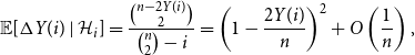 \begin{equation} \mathbb {E}[ \Delta Y(i) \mid {\mathcal {H}}_i] = \frac {\binom {n-2Y(i)}{2}}{\binom n2 - i} = \left (1 - \frac {2 Y(i)}{n}\right )^{2} + O\left (\frac 1n \right ), \end{equation}
where
 $\Delta Y(i)\,:\!=\, Y(i+1) - Y(i)$
, and the asymptotics are as
$\Delta Y(i)\,:\!=\, Y(i+1) - Y(i)$
, and the asymptotics are as
 $n \rightarrow \infty$
(which will be the case for the remainder of this note). By scaling
$n \rightarrow \infty$
(which will be the case for the remainder of this note). By scaling
 $(Y(i))_{i=0}^{m}$
by
$(Y(i))_{i=0}^{m}$
by
 $n$
, we can interpret the left-hand side of (1) as the ‘derivative’ of
$n$
, we can interpret the left-hand side of (1) as the ‘derivative’ of
 $Y(i)/n$
evaluated at
$Y(i)/n$
evaluated at
 $i/n$
. This suggests the following differential equation:
$i/n$
. This suggests the following differential equation:
 \begin{equation} y^{\prime}(t) = (1-2y(t))^2, \qquad y(0)=0 \end{equation}
with initial condition
 $y(0)=0$
. Wormald’s differential equation method allows us to conclude that with high probability (i.e. with probability tending to
$y(0)=0$
. Wormald’s differential equation method allows us to conclude that with high probability (i.e. with probability tending to
 $1$
as
$1$
as
 $n \rightarrow \infty$
, henceforth abbreviated whp.),
$n \rightarrow \infty$
, henceforth abbreviated whp.),
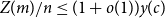
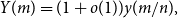 \begin{equation} Y(m) = (1 + o(1)) y(m/n), \end{equation}
where
 $y(t) \,:\!=\, t/(1+2t)$
is the unique solution to (2).
$y(t) \,:\!=\, t/(1+2t)$
is the unique solution to (2).
Returning to the general set-up of the differential equation method, suppose we are given a sequence of random variables
 $(Y(i))_{i=0}^{\infty }$
, which implicitly depend on
$(Y(i))_{i=0}^{\infty }$
, which implicitly depend on
 $n \in \mathbb {N}$
. Assume that the one-step changes are bounded; that is, there exists a constant
$n \in \mathbb {N}$
. Assume that the one-step changes are bounded; that is, there exists a constant
 $\beta \ge 0$
such that
$\beta \ge 0$
such that
 $|\Delta Y(i)| \le \beta$
for each
$|\Delta Y(i)| \le \beta$
for each
 $i \ge 0$
. Moreover, suppose each
$i \ge 0$
. Moreover, suppose each
 $Y(i)$
is determined by some sigma-algebra
$Y(i)$
is determined by some sigma-algebra
 $\mathcal {H}_i$
, and its expected one-step changes are described by some Lipschitz function
$\mathcal {H}_i$
, and its expected one-step changes are described by some Lipschitz function
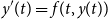
 $f=f(t,y)$
. That is, for each
$f=f(t,y)$
. That is, for each
 $i \ge 0$
,
$i \ge 0$
,
 \begin{equation} \mathbb {E}[\Delta Y(i) \mid \mathcal {H}_i] = f(i/n, Y(i)/n) + o(1). \end{equation}
If
 $Y(0) = (1 +o (1)) \widetilde {y} n$
for some constant
$Y(0) = (1 +o (1)) \widetilde {y} n$
for some constant
 $\widetilde {y}$
, and
$\widetilde {y}$
, and
 $m=m(n)$
is not too large, then the differential equation method allows us to conclude that whp
$m=m(n)$
is not too large, then the differential equation method allows us to conclude that whp
 $Y(m) /n = (1 + o(1)) y(m/n)$
for
$Y(m) /n = (1 + o(1)) y(m/n)$
for
 $y$
, which satisfies the differential equation suggested by (4), that is,
$y$
, which satisfies the differential equation suggested by (4), that is,
 \begin{equation*} y^{\prime}(t) = f(t, y(t)) \end{equation*}
with initial condition
 $y(0) = \widetilde {y}$
. In this note, we consider the case when we have an inequality in place of (4). We are motivated by applications to online algorithms in which one wishes to upper bound the performance of any online algorithm, opposed to just a particular algorithm. (See Section 1.1 for an example pertaining to online matching in
$y(0) = \widetilde {y}$
. In this note, we consider the case when we have an inequality in place of (4). We are motivated by applications to online algorithms in which one wishes to upper bound the performance of any online algorithm, opposed to just a particular algorithm. (See Section 1.1 for an example pertaining to online matching in
 $(G_i)_{i=0}^m$
as well as some discussion of further applications.) We are also motivated by the existence of deterministic results of which we wanted to prove a random analogue. For example, consider the following classical result due to Petrovitch [Reference Petrovitch10]:
$(G_i)_{i=0}^m$
as well as some discussion of further applications.) We are also motivated by the existence of deterministic results of which we wanted to prove a random analogue. For example, consider the following classical result due to Petrovitch [Reference Petrovitch10]:
Theorem 1.
Suppose
 $f\,:\,\mathbb {R}^2 \rightarrow \mathbb {R}$
is Lipschitz continuous, and
$f\,:\,\mathbb {R}^2 \rightarrow \mathbb {R}$
is Lipschitz continuous, and
 $y=y(t)$
satisfies
$y=y(t)$
satisfies
 \begin{equation*} y^{\prime}(t) = f(t, y(t)), \qquad y(c) = y_0. \end{equation*}
Suppose
 $z=z(t)$
is differentiable and satisfies
$z=z(t)$
is differentiable and satisfies
 \begin{equation*} z^{\prime}(t) \le f(t, z(t)), \qquad z(c) = z_0 \le y_0. \end{equation*}
Then
 $z(t) \le y(t)$
for all
$z(t) \le y(t)$
for all
 $t \ge c$
.
$t \ge c$
.
With the above result in mind (as well as the standard differential equation method), it’s natural to wonder what can be said about a sequence of random variables
 $(Z_i)_{i=1}^\infty$
satisfying
$(Z_i)_{i=1}^\infty$
satisfying
 \begin{equation*} \mathbb {E}[\Delta Z_i \mid \mathcal {H}_i] \le f(i/n, Z_i/n) \end{equation*}
instead of the equality version (4). More precisely, if
 $(Y_i)_{i=1}^\infty$
satisfies (4) and
$(Y_i)_{i=1}^\infty$
satisfies (4) and
 $Z_0 \lt Y_0$
, then should it not follow that we likely have
$Z_0 \lt Y_0$
, then should it not follow that we likely have
 $Z_i \le Y_i$
(perhaps modulo some relatively small error term) for all
$Z_i \le Y_i$
(perhaps modulo some relatively small error term) for all
 $i \ge 0$
?
$i \ge 0$
?
We briefly point out that if
 $f$
is nonincreasing in its second variable, then the problem described in the previous paragraph is much easier. Indeed, whenever the random variable satisfies
$f$
is nonincreasing in its second variable, then the problem described in the previous paragraph is much easier. Indeed, whenever the random variable satisfies
 $Z_i - Y_i \le 0$
, it is also a supermartingale. More precisely, when
$Z_i - Y_i \le 0$
, it is also a supermartingale. More precisely, when
 $Z_i \le Y_i$
, we have that
$Z_i \le Y_i$
, we have that
 \begin{equation*} \mathbb {E}[\Delta (Z_i - Y_i) \mid {\mathcal {H}}_i] \le f(i/n, Z_i/n) - f(i/n, Y_i/n) \le 0 \end{equation*}
by the monotonicity assumption. In this case, assuming the initial gap
 $|Z_0-Y_0|$
is large enough, standard martingale techniques can be used to bound the probability that the supermartingale
$|Z_0-Y_0|$
is large enough, standard martingale techniques can be used to bound the probability that the supermartingale
 $Z_i - Y_i$
becomes positive. However, we would like to handle applications where we do not have this monotonicity assumption. For instance, in our running example,
$Z_i - Y_i$
becomes positive. However, we would like to handle applications where we do not have this monotonicity assumption. For instance, in our running example,
 $f(t,z) = (1 -2z)^2$
is not increasing in
$f(t,z) = (1 -2z)^2$
is not increasing in
 $z$
.
$z$
.
Of course, the differential equation method in general deals with systems of random variables (and the associated systems of differential equations). So what can be said about systems of deterministic functions whose derivatives satisfy inequalities instead? It turns out that to generalise Theorem1 to a system, we need the functions to be cooperative. We say the functions
 $f_j\,:\!=\,\mathbb {R}^{a+1} \rightarrow \mathbb {R}, 1 \le j \le a$
are cooperative (respectively, competitive) if each
$f_j\,:\!=\,\mathbb {R}^{a+1} \rightarrow \mathbb {R}, 1 \le j \le a$
are cooperative (respectively, competitive) if each
 $f_j$
is nondecreasing (respectively, nonincreasing) in all of its
$f_j$
is nondecreasing (respectively, nonincreasing) in all of its
 $a+1$
inputs except for possibly the first input and the
$a+1$
inputs except for possibly the first input and the
 $(j+1)^{th}$
one. In other words,
$(j+1)^{th}$
one. In other words,
 $f_j(t, y_1, \ldots y_a)$
is nondecreasing in all variables except possibly
$f_j(t, y_1, \ldots y_a)$
is nondecreasing in all variables except possibly
 $t$
and
$t$
and
 $y_j$
. Note that some sources refer to a system with the cooperative property as being quasimonotonic. Observe that in the one-dimensional case
$y_j$
. Note that some sources refer to a system with the cooperative property as being quasimonotonic. Observe that in the one-dimensional case
 $a=1$
, every function is cooperative/cooperate. The following theorem is folklore (see [Reference Walter12] for some relevant background and Section 3 for a proof):
$a=1$
, every function is cooperative/cooperate. The following theorem is folklore (see [Reference Walter12] for some relevant background and Section 3 for a proof):
Theorem 2.
Suppose
 $f_j\,:\,\mathbb {R}^{a+1} \rightarrow \mathbb {R}, 1 \le j \le a$
are Lipschitz continuous and cooperative, and
$f_j\,:\,\mathbb {R}^{a+1} \rightarrow \mathbb {R}, 1 \le j \le a$
are Lipschitz continuous and cooperative, and
 $y_j$
satisfies
$y_j$
satisfies
 \begin{equation*} y_j^{\prime}(t) = f_j(t, y_1(t), \ldots, y_a(t)),\qquad 1 \le j \le a,\quad t \ge c. \end{equation*}
Suppose
 $z_j, 1 \le j \le a$
are differentiable and satisfy
$z_j, 1 \le j \le a$
are differentiable and satisfy
 $z_j(c) \le y_j(c)$
and
$z_j(c) \le y_j(c)$
and
 \begin{equation*} z_j^{\prime}(t) \le f_j(t, z_1(t), \ldots, z_a(t)), \qquad 1 \le j \le a,\quad t \ge c. \end{equation*}
Then
 $z_j(t) \le y_j(t)$
for all
$z_j(t) \le y_j(t)$
for all
 $1 \le j \le a$
,
$1 \le j \le a$
,
 $t \ge c.$
Cooperativity is necessary in the sense that if we do not have it, then one can choose initial conditions for the functions
 $y_j, z_j$
to make the conclusion of Theorem2 fail. Indeed, suppose we do not have cooperativity; that is, there exist
$y_j, z_j$
to make the conclusion of Theorem2 fail. Indeed, suppose we do not have cooperativity; that is, there exist
 $j, j^{\prime}$
with
$j, j^{\prime}$
with
 $j^{\prime} \neq j+1$
and some points
$j^{\prime} \neq j+1$
and some points
 $\textbf { p}, \textbf { p}^{\prime} \in \mathbb {R}^{a+1}$
that agree everywhere except for their
$\textbf { p}, \textbf { p}^{\prime} \in \mathbb {R}^{a+1}$
that agree everywhere except for their
 $j^{\prime th}$
coordinate, where we have
$j^{\prime th}$
coordinate, where we have
 $p_{j^{\prime}} \gt p_{j^{\prime}}^{\prime}$
and
$p_{j^{\prime}} \gt p_{j^{\prime}}^{\prime}$
and
 $f_j(\textbf { p}) \lt f_j(\bf {p^{\prime}})$
. Consider the following initial conditions:
$f_j(\textbf { p}) \lt f_j(\bf {p^{\prime}})$
. Consider the following initial conditions:
 \begin{equation*} \left (c, y_1(c), \ldots, y_a(c)\right ) = \textbf { p}, \qquad \left (c, z_1(c), \ldots, z_a(c)\right ) = \textbf { p}^{\prime}. \end{equation*}
Then we have that
 $z_j(c) = y_j(c) = p_{j+1} = p^{\prime}_{j+1}$
. Furthermore,
$z_j(c) = y_j(c) = p_{j+1} = p^{\prime}_{j+1}$
. Furthermore,
 $z_j^{\prime}(c)$
could be as large as
$z_j^{\prime}(c)$
could be as large as
 $f_j(\textbf { p}^{\prime}) \gt f_j(\textbf { p}) = y_j^{\prime}(c)$
in which case clearly
$f_j(\textbf { p}^{\prime}) \gt f_j(\textbf { p}) = y_j^{\prime}(c)$
in which case clearly
 $z_j(t) \gt y_j(t)$
for some
$z_j(t) \gt y_j(t)$
for some
 $t\gt c$
.
$t\gt c$
.
Our main theorem in this paper, Theorem3, is essentially the random analogue of Theorem2. Before providing its formal statement, we expand upon why it is useful for proving impossibility/hardness results for online algorithms. The reader can safely skip Section 1.1 if they would first like to instead read Theorem3.
1.1 Motivating applications
The example considered in this section is closely related to the
 $1/2$
-impossibility (or hardness) result for an online stochastic matching problem considered by the second author, Ma and Grammel in Theorem
$1/2$
-impossibility (or hardness) result for an online stochastic matching problem considered by the second author, Ma and Grammel in Theorem
 $5$
of [Reference MacRury, Ma and Grammel9]. In fact, Theorem3 is explicitly used to prove this result, and it is also applied in a similar way to prove Theorem
$5$
of [Reference MacRury, Ma and Grammel9]. In fact, Theorem3 is explicitly used to prove this result, and it is also applied in a similar way to prove Theorem
 $1.4$
of [Reference MacRury, Ma, Mohar, Shinkar and O’Donnell8]. Our theorem can also be used to simplify the proofs of the
$1.4$
of [Reference MacRury, Ma, Mohar, Shinkar and O’Donnell8]. Our theorem can also be used to simplify the proofs of the
 $\frac {1}{2}(1 + e^{-2})$
-impossibility result of Fu, Tang, Wu, Wu, and Zhang (Theorem
$\frac {1}{2}(1 + e^{-2})$
-impossibility result of Fu, Tang, Wu, Wu, and Zhang (Theorem
 $2$
in [Reference Fu, Tang, Wu, Wu, Zhang, Bansal, Merelli and Worell6]), and the
$2$
in [Reference Fu, Tang, Wu, Wu, Zhang, Bansal, Merelli and Worell6]), and the
 $1-\ln (2-1/e)$
-impossibility result of Fata, Ma, and Simchi-Levi (Lemma
$1-\ln (2-1/e)$
-impossibility result of Fata, Ma, and Simchi-Levi (Lemma
 $5$
in [Reference Fata, Ma and Simchi-Levi3]). All of the aforementioned papers prove impossibility results for various online stochastic optimisation problems – more specifically, hardness results for online contention resolution schemes [Reference Feldman, Svensson and Zenklusen4] or prophet inequalities against an ‘ex-ante relaxation’ [Reference Lee, Singla, Azar, Bast and Herman7]. We think that Theorem3 will find further applications as a technical tool in this area.
$5$
in [Reference Fata, Ma and Simchi-Levi3]). All of the aforementioned papers prove impossibility results for various online stochastic optimisation problems – more specifically, hardness results for online contention resolution schemes [Reference Feldman, Svensson and Zenklusen4] or prophet inequalities against an ‘ex-ante relaxation’ [Reference Lee, Singla, Azar, Bast and Herman7]. We think that Theorem3 will find further applications as a technical tool in this area.
Let us now return to the definition of the Erdős-Rényi random graph process
 $(G_i)_{i=0}^m$
as discussed in Section 1, where we again assume that
$(G_i)_{i=0}^m$
as discussed in Section 1, where we again assume that
 $m = c n$
for some constant
$m = c n$
for some constant
 $c \gt 0$
. Recall that (3) says that if
$c \gt 0$
. Recall that (3) says that if
 $Y(m)$
is the size of the matching constructed by the greedy matching algorithm when executed on
$Y(m)$
is the size of the matching constructed by the greedy matching algorithm when executed on
 $(G_i)_{i=0}^m$
, then whp
$(G_i)_{i=0}^m$
, then whp
 $Y(m)/n = (1 + o(1)) y(c)$
where
$Y(m)/n = (1 + o(1)) y(c)$
where
 $y(c) = c/(1+2c)$
. In fact, (3) can be made to hold with probability
$y(c) = c/(1+2c)$
. In fact, (3) can be made to hold with probability
 $1 - o(1/n^2)$
, and so
$1 - o(1/n^2)$
, and so
 $\mathbb {E}[ Y(m) ]/n = (1 +o(1)) c/(1+2c)$
after taking expectations.
$\mathbb {E}[ Y(m) ]/n = (1 +o(1)) c/(1+2c)$
after taking expectations.
The greedy matching algorithm is an example of an online (matching) algorithm on
 $(G_i)_{i=0}^m$
. An online algorithm begins with the empty matching on
$(G_i)_{i=0}^m$
. An online algorithm begins with the empty matching on
 $G_0$
, and its goal is to build a matching of
$G_0$
, and its goal is to build a matching of
 $G_{m}$
. While it knows the distribution of
$G_{m}$
. While it knows the distribution of
 $(G_i)_{i=0}^m$
upfront, it learns the instantiations of the edges sequentially and must execute online. Formally, in each step
$(G_i)_{i=0}^m$
upfront, it learns the instantiations of the edges sequentially and must execute online. Formally, in each step
 $i \ge 1$
, it is presented
$i \ge 1$
, it is presented
 $e_i$
and then makes an irrevocable decision as to whether or not to include
$e_i$
and then makes an irrevocable decision as to whether or not to include
 $e_i$
in its current matching, based upon
$e_i$
in its current matching, based upon
 $e_1, \ldots, e_{i-1}$
and its previous matching decisions. Its output is the matching
$e_1, \ldots, e_{i-1}$
and its previous matching decisions. Its output is the matching
 $M_m$
, and its goal is to maximise
$M_m$
, and its goal is to maximise
 $\mathbb {E}[ |M_m|]$
. Here the expectation is over
$\mathbb {E}[ |M_m|]$
. Here the expectation is over
 $(G_i)_{i=1}^{m}$
and any randomised decisions made by the algorithm.
$(G_i)_{i=1}^{m}$
and any randomised decisions made by the algorithm.
Suppose that we wish to prove that the greedy algorithm is asymptotically optimal. That is, for any online algorithm, if
 $M_m$
is the matching it outputs on
$M_m$
is the matching it outputs on
 $G_m$
, then
$G_m$
, then
 $\mathbb {E}[ |M_m|] \le (1 +o(1)) \mathbb {E}[ Y(m)]$
. In order to prove this directly, one must compare the performance of any online algorithm to the greedy algorithm. This is inconvenient to argue, as there exist rare instantiations of
$\mathbb {E}[ |M_m|] \le (1 +o(1)) \mathbb {E}[ Y(m)]$
. In order to prove this directly, one must compare the performance of any online algorithm to the greedy algorithm. This is inconvenient to argue, as there exist rare instantiations of
 $(G_i)_{i=0}^{m}$
in which being greedy is clearly suboptimal.
$(G_i)_{i=0}^{m}$
in which being greedy is clearly suboptimal.
We instead upper bound the performance of any online algorithm by
 $(1 + o(1)) y(c) n$
. Let
$(1 + o(1)) y(c) n$
. Let
 $(M_i)_{i=0}^{m}$
be the sequence of matchings constructed by an arbitrary online algorithm while executing on
$(M_i)_{i=0}^{m}$
be the sequence of matchings constructed by an arbitrary online algorithm while executing on
 $(G_i)_{i=0}^{m}$
. For simplicity, assume that the algorithm is deterministic so that
$(G_i)_{i=0}^{m}$
. For simplicity, assume that the algorithm is deterministic so that
 $M_i$
is
$M_i$
is
 $\mathcal {H}_i$
-measurable. In this case, we can replace (1) with inequality. That is, if
$\mathcal {H}_i$
-measurable. In this case, we can replace (1) with inequality. That is, if
 $Z(i)\,:\!=\,|M_i|$
, then for
$Z(i)\,:\!=\,|M_i|$
, then for
 $i \lt m$
,
$i \lt m$
,
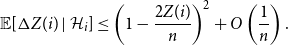 \begin{equation} \mathbb {E}[ \Delta Z(i) \mid \mathcal {H}_i] \le \left (1 - \frac {2Z(i)}{n}\right )^{2} + O\left (\frac 1n\right ). \end{equation}
Recall now the intuition behind the differential equation method. If we scale
 $(Z(i))_{i=0}^{n}$
by
$(Z(i))_{i=0}^{n}$
by
 $n$
, then we can interpret the left-hand side of (5) as the ‘derivative’ of
$n$
, then we can interpret the left-hand side of (5) as the ‘derivative’ of
 $Z(i)/n$
evaluated at
$Z(i)/n$
evaluated at
 $i/n$
. This suggests the following differential inequality:
$i/n$
. This suggests the following differential inequality:
 \begin{equation*} z^{\prime} \le (1 - 2z)^2, \end{equation*}
with inital condition
 $z(0)=0$
. By applying Theorem3 to
$z(0)=0$
. By applying Theorem3 to
 $(Z(i))_{i=0}^{m}$
, we get that
$(Z(i))_{i=0}^{m}$
, we get that
 \begin{equation*} Z(m)/n \le (1+ o(1)) y(c) \end{equation*}
with probability
 $1 - o(n^{-2})$
. As a result,
$1 - o(n^{-2})$
. As a result,
 $\mathbb {E}[ Z(m)] \le (1 +o(1)) y(c) n$
, and so we can conclude that greedy is asymptotically optimal.
$\mathbb {E}[ Z(m)] \le (1 +o(1)) y(c) n$
, and so we can conclude that greedy is asymptotically optimal.
2. Main theorem
For any sequence
 $(Z(i))_{i=0}^{\infty }$
of random variables and
$(Z(i))_{i=0}^{\infty }$
of random variables and
 $i \ge 0$
, we will use the notation
$i \ge 0$
, we will use the notation
 $\Delta Z(i) \,:\!=\, Z(i+1)-Z(i)$
. Note that given a filtration
$\Delta Z(i) \,:\!=\, Z(i+1)-Z(i)$
. Note that given a filtration
 $(\mathcal {H}_i)_{i=0}^{\infty }$
(i.e. a sequence of increasing
$(\mathcal {H}_i)_{i=0}^{\infty }$
(i.e. a sequence of increasing
 $\sigma$
-algebras), we say that
$\sigma$
-algebras), we say that
 $(Z_j(i))_{i= 0}^\infty$
is adapted to
$(Z_j(i))_{i= 0}^\infty$
is adapted to
 $(\mathcal {H}_i)_{i=0}^{\infty }$
, provided
$(\mathcal {H}_i)_{i=0}^{\infty }$
, provided
 $Z_i$
is
$Z_i$
is
 $\mathcal {H}_i$
-measurable for each
$\mathcal {H}_i$
-measurable for each
 $i \ge 0$
. Finally, we say that a stopping time
$i \ge 0$
. Finally, we say that a stopping time
 $I$
is adapted to
$I$
is adapted to
 $(\mathcal {H}_i)_{i=0}^{\infty }$
, provided the event
$(\mathcal {H}_i)_{i=0}^{\infty }$
, provided the event
 $\{I=i\}$
is
$\{I=i\}$
is
 $\mathcal {H}_i$
-measurable for each
$\mathcal {H}_i$
-measurable for each
 $i \ge 0$
.
$i \ge 0$
.
Given
 $a \in \mathbb {N}$
, suppose that
$a \in \mathbb {N}$
, suppose that
 $\mathcal {D} \subseteq \mathbb {R}^{a+1}$
is a bounded domain, and for
$\mathcal {D} \subseteq \mathbb {R}^{a+1}$
is a bounded domain, and for
 $1 \le j \le a$
, let
$1 \le j \le a$
, let
 $f_j\,:\, \mathcal {D} \rightarrow \mathbb {R}$
. We assume that the following hold for each
$f_j\,:\, \mathcal {D} \rightarrow \mathbb {R}$
. We assume that the following hold for each
 $j$
:
$j$
:
-
(a)
 $f_j$
is
$L$
-Lipschitz on
$\mathcal {D}$
, that is,
\begin{equation*} |f_j(t, y_1, \ldots, y_a) - f_j(t^{\prime}, y^{\prime}_1, \ldots, y^{\prime}_a) | \le L \cdot \max \{|t-t^{\prime}|, |y_1-y^{\prime}_1|, \ldots, |y_a-y^{\prime}_a|\} \end{equation*}
$f_j$
is
$L$
-Lipschitz on
$\mathcal {D}$
, that is,
\begin{equation*} |f_j(t, y_1, \ldots, y_a) - f_j(t^{\prime}, y^{\prime}_1, \ldots, y^{\prime}_a) | \le L \cdot \max \{|t-t^{\prime}|, |y_1-y^{\prime}_1|, \ldots, |y_a-y^{\prime}_a|\} \end{equation*}
-
(b)
$|f_j|\le B$
on
$\mathcal {D}$
, and -
(c) the
$(f_j)_{j=1}^a$
are cooperative.


Given
 $(0,{\tilde y}_1, \ldots, {\tilde y}_a) \in \mathcal {D}$
, assume that
$(0,{\tilde y}_1, \ldots, {\tilde y}_a) \in \mathcal {D}$
, assume that
 $y_1(t), \ldots, y_a(t)$
is the (unique) solution to the system:
$y_1(t), \ldots, y_a(t)$
is the (unique) solution to the system:
 \begin{equation} y_j^{\prime}(t) = f_j(t, y_1(t), \ldots, y_a(t)), \qquad y_j(0)={\tilde y}_j \end{equation}
for all
 $t \in [0, \sigma ]$
, where
$t \in [0, \sigma ]$
, where
 $\sigma$
is any positive value.
$\sigma$
is any positive value.
Theorem 3.
Suppose that for each
 $1 \le j \le a$
, we have a sequence of random variables
$1 \le j \le a$
, we have a sequence of random variables
 $(Z_j(i))_{i= 0}^\infty$
, which is adapted to some filtration
$(Z_j(i))_{i= 0}^\infty$
, which is adapted to some filtration
 $({\mathcal {H}}_i)_{i=0}^\infty$
. Let
$({\mathcal {H}}_i)_{i=0}^\infty$
. Let
 $n \in \mathbb {N}$
, and
$n \in \mathbb {N}$
, and
 $\beta, b, \lambda, \delta \gt 0$
be any parameters such that
$\beta, b, \lambda, \delta \gt 0$
be any parameters such that
 $\lambda \ge \max \left \{ \beta + B, \frac {L+BL + \delta n}{3L}\right \}$
. Given an arbitrary stopping time
$\lambda \ge \max \left \{ \beta + B, \frac {L+BL + \delta n}{3L}\right \}$
. Given an arbitrary stopping time
 $I \ge 0$
adapted to
$I \ge 0$
adapted to
 $({\mathcal {H}}_i)_{i=0}^\infty$
, suppose that the following properties hold for each
$({\mathcal {H}}_i)_{i=0}^\infty$
, suppose that the following properties hold for each
 $ 0 \le i \lt \min \{I, \sigma n \}$
:
$ 0 \le i \lt \min \{I, \sigma n \}$
:
-
1. The ‘Boundedness Hypothesis’:
$\max _{j} |\Delta Z_j(i)| \le \beta$
, and
$\max _{j} \mathbb {E}[ ( \Delta Z_{j}(i) )^2 \mid \mathcal {H}_i] \le b$
-
2. The ‘Trend Hypothesis’:
$(i/n, Z_1(i)/n, \ldots Z_a(i)/n) \in \mathcal {D}$
and
for each
\begin{equation*}\mathbb {E}[ \Delta Z_j(i) \mid {\mathcal {H}}_i] \le f_j(i/n, Z_1(i)/n, \ldots Z_a(i)/n) + \delta \end{equation*}
$1 \le j \le a$
.
-
3. The ‘Initial Condition’:
$Z_j(0) \le y_j(0) n + \lambda$
for all
$1 \le j \le a$
.


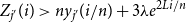
Then, with probability at least
 $1 - 2 a \exp \left ( -\frac {\lambda ^2}{2( b \sigma n + 2\beta \lambda )} \right )$
,
$1 - 2 a \exp \left ( -\frac {\lambda ^2}{2( b \sigma n + 2\beta \lambda )} \right )$
,
 \begin{equation*} Z_j(i) \le ny_{j}(i/n) + 3 \lambda e^{2L i/n} \end{equation*}
for all
 $1 \le j \le a$
and
$1 \le j \le a$
and
 $0 \le i \le \min \{I, \sigma n\}$
.
$0 \le i \le \min \{I, \sigma n\}$
.
Remark 4 (Simplified Parameters). By taking
 $b = \beta ^2$
and
$b = \beta ^2$
and
 $I = \lceil \sigma n \rceil$
, we can recover a simpler version of the theorem, which is sufficient for many applications, including the motivating example of Section 1.1.
$I = \lceil \sigma n \rceil$
, we can recover a simpler version of the theorem, which is sufficient for many applications, including the motivating example of Section 1.1.
Remark 5 (Stopping Time Selection). Let
 $0 \le \gamma \le 1$
be an additional parameter to Theorem 3. The stopping time
$0 \le \gamma \le 1$
be an additional parameter to Theorem 3. The stopping time
 $I$
is most commonly applied in the following way. Suppose that
$I$
is most commonly applied in the following way. Suppose that
 $(\mathcal {E}_i)_{i=0}^{\infty }$
is a sequence of events adapted to
$(\mathcal {E}_i)_{i=0}^{\infty }$
is a sequence of events adapted to
 $(\mathcal {H}_i)_{i=0}^{\infty }$
, and for each
$(\mathcal {H}_i)_{i=0}^{\infty }$
, and for each
 $0 \le i \lt \sigma n$
, Conditions 1 and 2 are only verified when
$0 \le i \lt \sigma n$
, Conditions 1 and 2 are only verified when
 $\mathcal {E}_i$
holds. Moreover, assume that
$\mathcal {E}_i$
holds. Moreover, assume that
 $\mathbb {P}[\cap _{i=0}^{\sigma n -1} \mathcal {E}_i] = 1 -\gamma$
. By defining
$\mathbb {P}[\cap _{i=0}^{\sigma n -1} \mathcal {E}_i] = 1 -\gamma$
. By defining
 $I$
to be the smallest
$I$
to be the smallest
 $i \ge 0$
such that
$i \ge 0$
such that
 $\mathcal {E}_i$
does not occur, Theorem 3 implies that with probability at least
$\mathcal {E}_i$
does not occur, Theorem 3 implies that with probability at least
 $1 - 2 a \exp \left ( -\frac {\lambda ^2}{2( b \sigma n + 2\beta \lambda )} \right ) - \gamma$
,
$1 - 2 a \exp \left ( -\frac {\lambda ^2}{2( b \sigma n + 2\beta \lambda )} \right ) - \gamma$
,
 \begin{equation*} Z_j(i) \le ny_{j}(i/n) + 3 \lambda e^{2L i/n} \end{equation*}
for all
 $1 \le j \le a$
and
$1 \le j \le a$
and
 $0 \le i \le \sigma n$
.
$0 \le i \le \sigma n$
.
Remark 6 (Competitive Functions). Theorem 3 yields upper bounds for families of random variables. There is a symmetric theorem for lower bounds, where all the appropriate inequalities are reversed and the functions
 $f_j$
are competitive instead of cooperative.
$f_j$
are competitive instead of cooperative.
We conclude the section with a corollary of Theorem3 which provides a useful extension of the theorem. Roughly speaking, the extension says that when verifying Conditions 1 and 2 at time
 $0 \le i \le \min \{\sigma n, I\}$
, it does not hurt to assume that (3) holds.
$0 \le i \le \min \{\sigma n, I\}$
, it does not hurt to assume that (3) holds.
Corollary 7 (of Theorem3). Suppose that in the terminology of Theorem 3, Conditions
1
and
2
are only verified for each
 $0 \le i \le \min \{I, \sigma n\}$
, which satisfies
$0 \le i \le \min \{I, \sigma n\}$
, which satisfies
 $Z_{j^{\prime}}(i) \le ny_{j^{\prime}}(i/n) + 3 \lambda e^{2Li/n}$
for all
$Z_{j^{\prime}}(i) \le ny_{j^{\prime}}(i/n) + 3 \lambda e^{2Li/n}$
for all
 $1 \le j^{\prime}\le a$
. In this case, the conclusion of Theorem 3 still holds. That is, with probability at least
$1 \le j^{\prime}\le a$
. In this case, the conclusion of Theorem 3 still holds. That is, with probability at least
 $1 - 2 a \exp \left ( -\frac {\lambda ^2}{2( b \sigma n + 2\beta \lambda )} \right )$
,
$1 - 2 a \exp \left ( -\frac {\lambda ^2}{2( b \sigma n + 2\beta \lambda )} \right )$
,
 \begin{equation*} Z_j(i) \le ny_{j}(i/n) + 3 \lambda e^{2L i/n} \end{equation*}
for all
 $1 \le j \le a$
and
$1 \le j \le a$
and
 $0 \le i \le \min \{I, \sigma n\}$
.
$0 \le i \le \min \{I, \sigma n\}$
.
Proof of Corollary
7
. Let
 $I^*$
be the first
$I^*$
be the first
 $i \ge 0$
such that
$i \ge 0$
such that
 \begin{equation*} Z_{j^{\prime}}(i) \gt ny_{j^{\prime}}(i/n) + 3 \lambda e^{2L i/n} \end{equation*}
for some
 $1 \le j^{\prime} \le a$
. Clearly,
$1 \le j^{\prime} \le a$
. Clearly,
 $I^*$
is a stopping time adapted to
$I^*$
is a stopping time adapted to
 $(\mathcal {H}_i)_{i=0}^{\infty }$
. Moreover, by the assumptions of the corollary, Conditions 1 and 2 hold for each
$(\mathcal {H}_i)_{i=0}^{\infty }$
. Moreover, by the assumptions of the corollary, Conditions 1 and 2 hold for each
 $0 \le i\le \min \{I^*, I, \sigma n\}$
and
$0 \le i\le \min \{I^*, I, \sigma n\}$
and
 $1 \le j \le a$
. Thus, Theorem3 implies that with probability at least
$1 \le j \le a$
. Thus, Theorem3 implies that with probability at least
 $1 - 2 a \exp \left ( -\frac {\lambda ^2}{2( b \sigma n + 2\beta \lambda )} \right )$
,
$1 - 2 a \exp \left ( -\frac {\lambda ^2}{2( b \sigma n + 2\beta \lambda )} \right )$
,
 \begin{equation*} Z_j(i) \le ny_{j}(i/n) + 3 \lambda e^{2L i/n} \end{equation*}
for all
 $1 \le j \le a$
and
$1 \le j \le a$
and
 $0 \le i \le \min \{I,I^*, \sigma n\}$
. Since the preceding event holds if and only if
$0 \le i \le \min \{I,I^*, \sigma n\}$
. Since the preceding event holds if and only if
 $I^* \gt \min \{I, \sigma n\}$
, the corollary is proven.
$I^* \gt \min \{I, \sigma n\}$
, the corollary is proven.
3. Proving Theorem 3
Before proceeding to the proof of Theorem3, we provide some intuition for our approach by presenting a proof of the deterministic setting (i.e. Theorem2). The notation and structure of the proof are intentionally chosen so as to relate to the analogous approach taken in the proof of Theorem3. Moreover, the main claim we prove can be viewed as an approximate version of Theorem2, in which the upper bounds on
 $z_{j}(0)$
and
$z_{j}(0)$
and
 $z^{\prime}_{j}$
only hold up to an additive constant
$z^{\prime}_{j}$
only hold up to an additive constant
 $\delta \gt 0$
.
$\delta \gt 0$
.
Proof of Theorem
2. Let us assume that
 $c=0$
is the boundary of the domain, and
$c=0$
is the boundary of the domain, and
 $L$
is a Lipschitz constant for the cooperative functions
$L$
is a Lipschitz constant for the cooperative functions
 $(f_j)_{j=1}^{a}$
. We shall prove the following: Given an arbitrary
$(f_j)_{j=1}^{a}$
. We shall prove the following: Given an arbitrary
 $\delta \gt 0$
, if
$\delta \gt 0$
, if
 \begin{equation} z_j^{\prime}(t) \le f(t, z_j(t))+\delta, \qquad z_j(0) \le y_j(0) +\delta \end{equation}
for all
 $1 \le j \le a$
and
$1 \le j \le a$
and
 $t \ge 0$
, then
$t \ge 0$
, then
 \begin{equation} z_{j}(t) \le y_{j}(t) + \delta e^{L t} \end{equation}
for each
 $1 \le j \le a$
and
$1 \le j \le a$
and
 $t \ge 0$
. Since (7) holds each
$t \ge 0$
. Since (7) holds each
 $\delta \gt 0$
under the assumptions of Theorem2, so must (8). This will imply that
$\delta \gt 0$
under the assumptions of Theorem2, so must (8). This will imply that
 $z_{j}(t) \le y_{j}(t)$
for each
$z_{j}(t) \le y_{j}(t)$
for each
 $1 \le j \le a$
and
$1 \le j \le a$
and
 $t \ge 0$
, thus completing the proof.
$t \ge 0$
, thus completing the proof.
In order to prove that (7) implies (8), define
 \begin{equation*} g(t)\,:\!=\, 2\delta e^{Lt}, \qquad s_j(t)\,:\!=\,z_j(t) - (y_j(t) +g(t)), \qquad I_j(t)\,:\!=\,[y_j(t), y_j(t) + g(t)). \end{equation*}
It suffices to show that
 $\max _{1 \le j \le a} s_j(t) \le 0$
for all
$\max _{1 \le j \le a} s_j(t) \le 0$
for all
 $t \ge 0$
. Observe first that
$t \ge 0$
. Observe first that
 $s_j(0)=z_{j}(0)-y_{j}(0)-g(0) \le -\delta \lt 0$
for all
$s_j(0)=z_{j}(0)-y_{j}(0)-g(0) \le -\delta \lt 0$
for all
 $1 \le j \le a$
. Suppose for the sake of contradiction that there exists some
$1 \le j \le a$
. Suppose for the sake of contradiction that there exists some
 $1 \le j^{\prime} \le a$
such that
$1 \le j^{\prime} \le a$
such that
 $s_{j^{\prime}}(t) \gt 0$
for some
$s_{j^{\prime}}(t) \gt 0$
for some
 $t \gt 0$
. In this case, there must be some value
$t \gt 0$
. In this case, there must be some value
 $t_1$
with
$t_1$
with
 $s_{j^{\prime}}(t_1)=0$
and
$s_{j^{\prime}}(t_1)=0$
and
 $\max _{1 \le j \le a} s_{j}(t)\lt 0$
for all
$\max _{1 \le j \le a} s_{j}(t)\lt 0$
for all
 $t \lt t_1$
. Furthermore, there must be some
$t \lt t_1$
. Furthermore, there must be some
 $t_0\lt t_1$
such that
$t_0\lt t_1$
such that
 $s_{j^{\prime}}(t) \in [-g(t), 0)$
for all
$s_{j^{\prime}}(t) \in [-g(t), 0)$
for all
 $t_0 \le t \lt t_1$
. Thus, for
$t_0 \le t \lt t_1$
. Thus, for
 $t_0 \le t \lt t_1$
, we have that
$t_0 \le t \lt t_1$
, we have that
 \begin{equation} -g(t) \le z_{j^{\prime}}(t) - [y_{j^{\prime}}(t) +g(t)] \lt 0 \qquad \Longrightarrow \qquad y_{j^{\prime}}(t) \le z_{j^{\prime}}(t) \lt y_{j^{\prime}}(t) + g(t), \end{equation}
and so
 \begin{align} f_{j^{\prime}}\left (t, z_1(t), \ldots z_a(t)\right ) & \le f_{j^{\prime}}\left (t, y_1(t)+g(t), \ldots, z_{j^{\prime}}(t), \ldots, y_a(t)+g(t)\right )\nonumber \\ & \le f_{j^{\prime}}\left (t, y_1(t), \ldots, y_a(t)\right ) + Lg(t) \end{align}
where the first line is by cooperativity of the functions
 $f_j$
and the second line is by the Lipschitzness of
$f_j$
and the second line is by the Lipschitzness of
 $f_{j^{\prime}}$
applied to (9). As such, for all
$f_{j^{\prime}}$
applied to (9). As such, for all
 $t \in [t_0, t_1)$
,
$t \in [t_0, t_1)$
,
 \begin{align*} s_{j^{\prime}}^{\prime}(t) &= z_{j^{\prime}}^{\prime}(t) - y_{j^{\prime}}^{\prime}(t) - g^{\prime}(t)\\ & = f_{j^{\prime}}\left (t, z_1(t), \ldots, z_a(t)\right ) - f_{j^{\prime}}\left (t, y_1(t), \ldots, y_a(t)\right ) -g^{\prime}(t)\\ &\le Lg(t) - g^{\prime}(t) =0 \end{align*}
where the last line uses (10). But now, we have a contradiction:
 $s_{j^{\prime}}(t_0) \in [{-}g(t_0), 0)$
, so it is negative,
$s_{j^{\prime}}(t_0) \in [{-}g(t_0), 0)$
, so it is negative,
 $s_{j^{\prime}}^{\prime}(t) \le 0$
on
$s_{j^{\prime}}^{\prime}(t) \le 0$
on
 $[t_0, t_1)$
, and yet
$[t_0, t_1)$
, and yet
 $s_{j^{\prime}}(t_1)=0$
.
$s_{j^{\prime}}(t_1)=0$
.
Our proof of Theorem3 is based partly on the critical interval method. Similar ideas were used by Telcs, Wormald, and Zhou [Reference Telcs, Wormald and Zhou11], as well as Bohman, Frieze, and Lubetzky [Reference Bohman, Frieze and Lubetzky2] (whose terminology we use here). For a gentle discussion of the method, see the paper of the first author and Dudek [Reference Bennett and Dudek1]. Roughly speaking, the critical interval method allows us to assume we have good estimates of key variables during the very steps that we are most concerned with those variables. Historically, this method has been used with more standard applications of the differential equation method in order to exploit self-correcting random variables; that is, a variable with the property that when it strays significantly from its trajectory, its expected one-step change makes it likely to move back towards its trajectory. For such a random variable, knowing that it lies in an interval strictly above (or below) the trajectory gives us a more favourable estimate for its expected one-step change. In our setting, we use the method for a similar but different reason. In particular, since we can only hope for one-sided bounds, we may as well ignore our random variables when they are far away from their bounds (in any case, we do not have or need good estimates for their expected one-step changes, etc., during the steps when all variables are far from their bounds).
We give an analogy. A rough proof sketch for Theorem2 is as follows: in order to have
 $z_j(t) \gt y_j(t)$
for some
$z_j(t) \gt y_j(t)$
for some
 $t$
, there must be some time interval during which
$t$
, there must be some time interval during which
 $z_j\approx y_j$
and during that interval
$z_j\approx y_j$
and during that interval
 $z_j$
must increase significantly faster than
$z_j$
must increase significantly faster than
 $y_j$
, which contradicts what we know about their derivatives. An analogous proof sketch for Theorem3 is as follows: in order for
$y_j$
, which contradicts what we know about their derivatives. An analogous proof sketch for Theorem3 is as follows: in order for
 $Z_j(i)$
to violate its upper bound, it must first enter a critical interval, which we will define to be near the upper bound, and then
$Z_j(i)$
to violate its upper bound, it must first enter a critical interval, which we will define to be near the upper bound, and then
 $Z_j$
must increase significantly (more than we expect it to) over the subsequent steps, which, while possible, is unlikely. Our probability bound will follow from Freedman’s inequality, which we will now state.
$Z_j$
must increase significantly (more than we expect it to) over the subsequent steps, which, while possible, is unlikely. Our probability bound will follow from Freedman’s inequality, which we will now state.
Theorem 8 (Freedman’s Inequality [Reference Freedman5]). Suppose that
 $(\mathcal {H}_i)_{i=0}^\infty$
is an increasing sequence of
$(\mathcal {H}_i)_{i=0}^\infty$
is an increasing sequence of
 $\sigma$
-algebras (i.e.
$\sigma$
-algebras (i.e.
 $\mathcal {H}_{i-1} \subseteq \mathcal {H}_{i}$
for all
$\mathcal {H}_{i-1} \subseteq \mathcal {H}_{i}$
for all
 $i \ge 1$
.) Moreover, let
$i \ge 1$
.) Moreover, let
 $(M_i)_{i=0}^\infty$
be a sequence of random variables adapted to
$(M_i)_{i=0}^\infty$
be a sequence of random variables adapted to
 $(\mathcal {H}_i)_{i=0}^\infty$
(i.e. each
$(\mathcal {H}_i)_{i=0}^\infty$
(i.e. each
 $M_i$
is
$M_i$
is
 $\mathcal {H}_i$
-measurable). Recall that
$\mathcal {H}_i$
-measurable). Recall that
 $\Delta M_{i}\,:\!=\, M_{i+1} -M_i$
and
$\Delta M_{i}\,:\!=\, M_{i+1} -M_i$
and
 ${\textbf { Var}}(\Delta M_i \mid \mathcal {H}_i)\,:\!=\, \mathbb {E}[ \Delta M_i^2 \mid \mathcal {H}_i] - \mathbb {E}[\Delta M_i \mid \mathcal {H}_i]^2$
for
${\textbf { Var}}(\Delta M_i \mid \mathcal {H}_i)\,:\!=\, \mathbb {E}[ \Delta M_i^2 \mid \mathcal {H}_i] - \mathbb {E}[\Delta M_i \mid \mathcal {H}_i]^2$
for
 $i \ge 0$
. Fix
$i \ge 0$
. Fix
 $m \in \mathbb {N}$
and
$m \in \mathbb {N}$
and
 $\beta, b \ge 0$
. Assume that for each
$\beta, b \ge 0$
. Assume that for each
 $0 \le i \lt m$
,
$0 \le i \lt m$
,
 $\mathbb {E}[\Delta M_i \mid \mathcal {H}_i] =0$
,
$\mathbb {E}[\Delta M_i \mid \mathcal {H}_i] =0$
,
 $|\Delta M_{i}| \le \beta$
, and
$|\Delta M_{i}| \le \beta$
, and
 ${\textbf { Var}}( \Delta M_i \mid \mathcal {H}_i) \le b$
. Then, for any
${\textbf { Var}}( \Delta M_i \mid \mathcal {H}_i) \le b$
. Then, for any
 $0 \lt \varepsilon \lt 1$
,
$0 \lt \varepsilon \lt 1$
,
 \begin{equation*} \mathbb {P}(\exists \; 0 \le i \le m \,:\, |M_i - M_0| \geq \varepsilon ) \leq \displaystyle 2\exp \left (-\frac {\varepsilon ^2}{2(b m + \beta \varepsilon ) }\right ). \end{equation*}
Moreover, if
 $I$
is an arbitrary stopping time adapted to
$I$
is an arbitrary stopping time adapted to
 $(\mathcal {H}_i)_{i=0}^{\infty }$
(i.e.
$(\mathcal {H}_i)_{i=0}^{\infty }$
(i.e.
 $\{I =i\}$
is
$\{I =i\}$
is
 $\mathcal {H}_i$
-measurable for each
$\mathcal {H}_i$
-measurable for each
 $i \ge 0$
), and the above conditions regarding
$i \ge 0$
), and the above conditions regarding
 $(M_i)_{i=0}^{\infty }$
are only verified for all
$(M_i)_{i=0}^{\infty }$
are only verified for all
 $0 \le i \lt \min \{I, m\}$
, then
$0 \le i \lt \min \{I, m\}$
, then
 \begin{equation*} \mathbb {P}(\exists \; 0 \le i \le \min \{I, m\} \,:\, |M_i - M_0| \geq \varepsilon ) \leq \displaystyle 2\exp \left (-\frac {\varepsilon ^2}{2(b m + \beta \varepsilon ) }\right ). \end{equation*}
Proof of Theorem
3
. Fix
 $0 \le i \le \sigma n$
, and set
$0 \le i \le \sigma n$
, and set
 $m\,:\!=\, \sigma n$
,
$m\,:\!=\, \sigma n$
,
 $t=t_i=i/n$
, and
$t=t_i=i/n$
, and
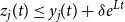
 $g(t)\,:\!=\, 3\lambda e^{2Lt}$
for convenience. Define
$g(t)\,:\!=\, 3\lambda e^{2Lt}$
for convenience. Define
 \begin{align*} S_j(i):&=Z_j(i)-(ny_j(t) + g(t)), \quad X_j(i)\,:\!=\,\sum _{k=0}^{i-1} \mathbb {E}[\Delta S_j(k) \mid {\mathcal {H}}_{k}], \\ M_j(i):&= S_j(0) + \sum _{k=0}^{i-1} \left (\Delta S_j(k)- \mathbb {E}[\Delta S_j(k) \mid {\mathcal {H}}_{k}]\right ), \end{align*}
so that
 $S_j(i) = X_j(i) + M_j(i)$
,
$S_j(i) = X_j(i) + M_j(i)$
,
 $(M_j(i))_{i= 0}^{m}$
is a martingale and
$(M_j(i))_{i= 0}^{m}$
is a martingale and
 $X_j(i)$
is
$X_j(i)$
is
 ${\mathcal {H}}_{i-1}$
-measurable (i.e.
${\mathcal {H}}_{i-1}$
-measurable (i.e.
 $(X_j(i) + M_j(i))_{i= 0}^{m}$
is the Doob decomposition of
$(X_j(i) + M_j(i))_{i= 0}^{m}$
is the Doob decomposition of
 $(S_j(i))_{i= 0}^{m}$
). Note that we can view
$(S_j(i))_{i= 0}^{m}$
). Note that we can view
 $S_{j}(i)/n$
as the random analogue of
$S_{j}(i)/n$
as the random analogue of
 $s_{j}(t) =m_{j}(t) + x_{j}(t)$
from the proof of Theorem2. In the previous deterministic setting, the decomposition
$s_{j}(t) =m_{j}(t) + x_{j}(t)$
from the proof of Theorem2. In the previous deterministic setting, the decomposition
 $s_{j}(t) =m_{j}(t) + x_{j}(t)$
is redundant, as
$s_{j}(t) =m_{j}(t) + x_{j}(t)$
is redundant, as
 $m_{j}(t) = s_{j}(0)$
, and so
$m_{j}(t) = s_{j}(0)$
, and so
 $x_{j}(t)$
and
$x_{j}(t)$
and
 $s_{j}(t)$
differ by a constant. In contrast,
$s_{j}(t)$
differ by a constant. In contrast,
 $M_{j}(i)$
is
$M_{j}(i)$
is
 $S_{j}(0)$
, plus
$S_{j}(0)$
, plus
 $\sum _{k=0}^{i-1} \left (\Delta S_j(k)- \mathbb {E}[\Delta S_j(k) \mid {\mathcal {H}}_{k}]\right )$
, the latter of which we can view as introducing some random noise. We handle this random noise by showing that
$\sum _{k=0}^{i-1} \left (\Delta S_j(k)- \mathbb {E}[\Delta S_j(k) \mid {\mathcal {H}}_{k}]\right )$
, the latter of which we can view as introducing some random noise. We handle this random noise by showing that
 $M_{j}(i)$
is typically concentrated about
$M_{j}(i)$
is typically concentrated about
 $S_{j}(0)$
due to Freedman’s inequality (see Theorem8). We refer to this as the probabilistic part of the proof. Assuming that this concentration holds, we can upper bound
$S_{j}(0)$
due to Freedman’s inequality (see Theorem8). We refer to this as the probabilistic part of the proof. Assuming that this concentration holds, we can upper bound
 $Z_{j}(i)$
by
$Z_{j}(i)$
by
 $ny_j(t) + g(t)$
via an argument that proceeds analogously to the proof of Theorem2. This is the deterministic part of the proof.
$ny_j(t) + g(t)$
via an argument that proceeds analogously to the proof of Theorem2. This is the deterministic part of the proof.
Beginning with the probabilistic part of the proof, we restrict our attention to
 $0 \le i \lt \min \{I, m\}$
. Observe first that
$0 \le i \lt \min \{I, m\}$
. Observe first that
 \begin{align*} \Delta M_j(i) &= \Delta S_j(i)- \mathbb {E}[\Delta S_j(i) \mid {\mathcal {H}}_{i}]\\ & = \Delta [Z_j(i)-(ny_j(t) + g(t))]- \mathbb {E}[\Delta [Z_j(i)-(ny_j(t) + g(t))] \mid {\mathcal {H}}_{i}]\\ & = \Delta Z_j(i)- \mathbb {E}[\Delta Z_j(i) \mid {\mathcal {H}}_{i}], \end{align*}
and so by Condition 1,
 \begin{equation*} |\Delta M_j(i)| \le |\Delta Z_j(i)| + |\mathbb {E}[\Delta Z_j(i) \mid {\mathcal {H}}_{i}]| \le 2 \beta . \end{equation*}
Also,
 ${\textbf { Var}}[ \Delta M_{j}(i) \mid \mathcal {H}_i] = \mathbb {E}[ (\Delta Z_j(i)- \mathbb {E}[\Delta Z_j(i) \mid \mathcal {H}_{i}])^2 \mid \mathcal {H}_i]$
. Thus,
${\textbf { Var}}[ \Delta M_{j}(i) \mid \mathcal {H}_i] = \mathbb {E}[ (\Delta Z_j(i)- \mathbb {E}[\Delta Z_j(i) \mid \mathcal {H}_{i}])^2 \mid \mathcal {H}_i]$
. Thus,
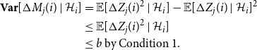 \begin{align*} {\textbf { Var}}[ \Delta M_{j}(i) \mid \mathcal {H}_i] &= \mathbb {E}[ \Delta Z_j(i)^2 \mid \mathcal {H}_i] - \mathbb {E}[\Delta Z_j(i) \mid {\mathcal {H}}_{i}]^2 \\ &\le \mathbb {E}[ \Delta Z_j(i)^2 \mid \mathcal {H}_i] \\ &\le b \text { by Condition 1. } \end{align*}
We can therefore apply Theorem8 to get that
 \begin{equation} \mathbb {P}(\exists \; 0 \le j \le a, 0 \le i \le \min \{I, m\} \,:\, |M_j(i) - M_j(0)| \ge \lambda ) \le 2a \exp \left ( -\frac {\lambda ^2}{2( b m + 2\beta \lambda )} \right ). \end{equation}
Suppose the above event does not happen; that is, for all
 $0 \le j \le a,0 \le i \le \min \{m,I\}$
, we have that
$0 \le j \le a,0 \le i \le \min \{m,I\}$
, we have that
 $|M_j(i) - M_j(0)| \lt \lambda$
. We will show that we also have
$|M_j(i) - M_j(0)| \lt \lambda$
. We will show that we also have
 $Z_j(i) \le ny_j(t)+g(t)$
for all
$Z_j(i) \le ny_j(t)+g(t)$
for all
 $0 \le i \le \min \{m,I\}$
and
$0 \le i \le \min \{m,I\}$
and
 $1 \le j \le a$
(equivalently,
$1 \le j \le a$
(equivalently,
 $\max _{j} S_{j}(i) \le 0$
for all
$\max _{j} S_{j}(i) \le 0$
for all
 $0 \le i \le \min \{m,I\}$
). This implication is the deterministic part of the proof. By combining it with the probability bound of (11), this will complete the proof of Theorem3.
$0 \le i \le \min \{m,I\}$
). This implication is the deterministic part of the proof. By combining it with the probability bound of (11), this will complete the proof of Theorem3.
Suppose for the sake of contradiction that
 $i^{\prime}$
is the minimal integer such that
$i^{\prime}$
is the minimal integer such that
 $0 \le i^{\prime} \le \min \{m,I\}$
and
$0 \le i^{\prime} \le \min \{m,I\}$
and
 $Z_j(i^{\prime}) \gt ny_j(t_{i^{\prime}})+g(t_{i^{\prime}})$
for some
$Z_j(i^{\prime}) \gt ny_j(t_{i^{\prime}})+g(t_{i^{\prime}})$
for some
 $j$
. Define the critical interval
$j$
. Define the critical interval
 \begin{equation*} I_j(i) \,:\!=\, \left [ ny_j(t), ny_j(t)+g(t)\right ]. \end{equation*}
First observe that since
 $g(0)\,:\!=\,3 \lambda \gt \lambda$
, Condition 3 implies that
$g(0)\,:\!=\,3 \lambda \gt \lambda$
, Condition 3 implies that
 $i^{\prime} \gt 0$
(and so
$i^{\prime} \gt 0$
(and so
 $i^{\prime}-1 \ge 0$
.) We claim that
$i^{\prime}-1 \ge 0$
.) We claim that
 $Z_j(i^{\prime}-1) \in I_j(i^{\prime}-1)$
. Indeed, note that by the minimality of
$Z_j(i^{\prime}-1) \in I_j(i^{\prime}-1)$
. Indeed, note that by the minimality of
 $i^{\prime}$
, we have that
$i^{\prime}$
, we have that
 $Z_j(i^{\prime}-1) \le ny_j(t_{i^{\prime}-1})+g(t_{i^{\prime}-1})$
. On the other hand,
$Z_j(i^{\prime}-1) \le ny_j(t_{i^{\prime}-1})+g(t_{i^{\prime}-1})$
. On the other hand,
 $|y_j^{\prime}| = |f_j| \le B$
and so each
$|y_j^{\prime}| = |f_j| \le B$
and so each
 $y_j$
is
$y_j$
is
 $B$
-Lipschitz. Thus, since
$B$
-Lipschitz. Thus, since
 $\lambda \ge \beta + B$
(by assumption),
$\lambda \ge \beta + B$
(by assumption),
 \begin{align*} Z_j(i^{\prime}-1) \ge Z_j(i^{\prime}) - \beta &\gt ny_j(t_{i^{\prime}})+g(t_{i^{\prime}}) - \beta \\ & \ge ny_j(t_{i^{\prime}-1}) +3\lambda - \beta - B \\ & \ge ny_j(t_{i^{\prime}-1}). \end{align*}
As a result,
 $Z_{j}(i^{\prime}-1) \in I_{j}(i^{\prime}-1)$
. Now let
$Z_{j}(i^{\prime}-1) \in I_{j}(i^{\prime}-1)$
. Now let
 $i^{\prime\prime} \le i^{\prime}-1$
be the minimal integer with the property that for all
$i^{\prime\prime} \le i^{\prime}-1$
be the minimal integer with the property that for all
 $i^{\prime\prime} \le i \le i^{\prime}-1$
, we have that
$i^{\prime\prime} \le i \le i^{\prime}-1$
, we have that
 $Z_j(i) \in I_j(i)$
. Then
$Z_j(i) \in I_j(i)$
. Then
 $Z_j(i^{\prime\prime}-1) \notin I_j(i^{\prime\prime}-1)$
, and by the minimality of
$Z_j(i^{\prime\prime}-1) \notin I_j(i^{\prime\prime}-1)$
, and by the minimality of
 $i^{\prime}$
, we must have that
$i^{\prime}$
, we must have that
 $Z_j(i^{\prime\prime}-1) \lt ny_j(t_{i^{\prime\prime}-1})$
. By once again using the fact that
$Z_j(i^{\prime\prime}-1) \lt ny_j(t_{i^{\prime\prime}-1})$
. By once again using the fact that
 $y_j$
is
$y_j$
is
 $B$
-Lipschitz,
$B$
-Lipschitz,
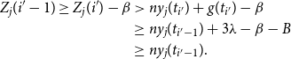
 \begin{align} Z_j(i^{\prime\prime}) \le Z_j(i^{\prime\prime}-1) + \beta & \lt ny_j(t_{i^{\prime\prime}-1}) + \beta \le ny_j(t_{i^{\prime\prime}}) + \beta +B. \end{align}
Now, since
 $Z_j(i^{\prime}) \gt ny_j(t_{i^{\prime}})+g(t_{i^{\prime}})$
, we can apply (12) to get that
$Z_j(i^{\prime}) \gt ny_j(t_{i^{\prime}})+g(t_{i^{\prime}})$
, we can apply (12) to get that
 \begin{align} S_j(i^{\prime}) - S_j(i^{\prime\prime}) &= (Z_j(i^{\prime}) - ny_j(t_{i^{\prime}}) -g(t_{i^{\prime}})) - (Z_j(i^{\prime\prime}) - ny_j(t_{i^{\prime\prime}}) - g(t_{i^{\prime\prime}}))\nonumber \\ &\gt g(t_{i^{\prime\prime}})-\beta -B \nonumber \\ &\ge 3 \lambda -\beta -B. \end{align}
Intuitively, (13) says that
 $S_{j}(i)$
increases significantly between steps
$S_{j}(i)$
increases significantly between steps
 $i^{\prime\prime}$
and
$i^{\prime\prime}$
and
 $i^{\prime}$
. We will now argue that
$i^{\prime}$
. We will now argue that
 $\mathbb {E}[ \Delta S_{j}(i) \mid {\mathcal {H}}_i]$
is nonpositive between steps
$\mathbb {E}[ \Delta S_{j}(i) \mid {\mathcal {H}}_i]$
is nonpositive between steps
 $i^{\prime\prime}$
and
$i^{\prime\prime}$
and
 $i^{\prime}$
. Informally, by scaling by
$i^{\prime}$
. Informally, by scaling by
 $n$
and interpreting
$n$
and interpreting
 $\mathbb {E}[ \Delta S_{j}(i) \mid {\mathcal {H}}_i]$
as the ‘derivative’ of
$\mathbb {E}[ \Delta S_{j}(i) \mid {\mathcal {H}}_i]$
as the ‘derivative’ of
 $S_{j}(i)/n$
evaluated at
$S_{j}(i)/n$
evaluated at
 $i/n$
, this will allow us to derive a contradiction in an analogous way as in the final part of the proof of Theorem2.
$i/n$
, this will allow us to derive a contradiction in an analogous way as in the final part of the proof of Theorem2.
Observe first that for each
 $i^{\prime\prime} \le i \le i^{\prime}-1$
, we have that
$i^{\prime\prime} \le i \le i^{\prime}-1$
, we have that
 \begin{align} \mathbb {E}[\Delta S_{j}(i) \mid {\mathcal {H}}_i] & = \mathbb {E}[ \Delta Z_{j}(i) \mid {\mathcal {H}}_i] - \Delta ny_j(t) - \Delta g(t)\nonumber \\ & \le f_j(t, Z_1(i)/n, \ldots Z_a(i)/n) + \delta \nonumber \\ & \qquad \qquad - f_j(t, y_1(t), \ldots, y_a(t)) + (L+BL)n^{-1} - n^{-1} g^{\prime}(t) \end{align}
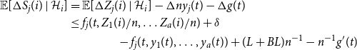
where the first line is by definition and line (14) will now be justified. The first two terms follow since by Condition 2,
 $(t, Z_1(i)/n, \ldots Z_a(i)/n) \in \mathcal {D}$
, and
$(t, Z_1(i)/n, \ldots Z_a(i)/n) \in \mathcal {D}$
, and
 \begin{equation*}\mathbb {E}[ \Delta Z_j(i) \mid {\mathcal {H}}_i] \le f_j(t, Z_1(i)/n, \ldots Z_a(i)/n) + \delta .\end{equation*}
For the third and fourth terms of (14), note that
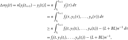 \begin{align} \Delta ny_j(t) = n[y_j(t_{i+1})-y_j(t_i)] &= n \int _{t_i}^{t_{i+1}} y_j^{\prime}(\tau ) \; d\tau \nonumber \\ & = n \int _{t_i}^{t_{i+1}} f_j(\tau, y_1(\tau ), \ldots, y_a(\tau )) \; d\tau \nonumber \\ & \ge n \int _{t_i}^{t_{i+1}} f_j(t, y_1(t_i), \ldots, y_a(t_i)) -(L+BL)n^{-1} \; d\tau \nonumber \\ & = f_j(t, y_1(t_i), \ldots, y_a(t_i))- (L+BL)n^{-1}, \end{align}
where (15) follows since for all
 $\tau \in [t_i, t_{i+1}]$
, we have
$\tau \in [t_i, t_{i+1}]$
, we have
 $|y_j(\tau ) - y_j(t_i)| \le B|\tau -t_i| \le Bn^{-1}$
(since the
$|y_j(\tau ) - y_j(t_i)| \le B|\tau -t_i| \le Bn^{-1}$
(since the
 $y_j$
are
$y_j$
are
 $B$
-Lipschitz), and now since the
$B$
-Lipschitz), and now since the
 $f_j$
are
$f_j$
are
 $L$
-Lipschitz, we have
$L$
-Lipschitz, we have
 \begin{equation*} |f_j(\tau, y_1(\tau ), \ldots, y_a(\tau )) - f_j(t, y_1(t_i), \ldots, y_a(t_i))| \le L \cdot \max \{|\tau -t_i|, Bn^{-1}\} \le L(1+B)n^{-1}. \end{equation*}
For the last term of (14), we have that
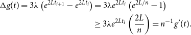 \begin{align*} \Delta g(t) = 3 \lambda \left (e^{2L t_{i+1}} - e^{2L t_{i}}\right ) &= 3 \lambda e^{2L t_{i}} \left (e^{2L /n} - 1\right )\\ & \ge 3\lambda e^{2L t_{i}} \left (\frac {2L}{n}\right ) = n^{-1}g^{\prime}(t). \end{align*}
Observe now that by cooperativity,
 $f_j(t, Z_1(i)/n, \ldots Z_a(i)/n)$
is upper bounded by
$f_j(t, Z_1(i)/n, \ldots Z_a(i)/n)$
is upper bounded by
 \begin{equation} f_j\left (t, \frac {ny_1(t)+g(t)}{n}, \ldots, \frac {ny_{j-1}(t)+g(t)}{n}, \frac {Z_j(i)}{n}, \frac {ny_{j+1}(t)+g(t)}{n}, \ldots, \frac {ny_a(t)+g(t)}{n}\right ). \end{equation}
Now, since
 $Z_j(i) \in I_j(i)$
, we can apply the Lipschitzness of
$Z_j(i) \in I_j(i)$
, we can apply the Lipschitzness of
 $f_j$
to (16) to get that
$f_j$
to (16) to get that
 \begin{equation} f_j(t, Z_1(i)/n, \ldots Z_a(i)/n) \le f_j(t, y_1(t), \ldots, y_a(t)) + L g(t)/n. \end{equation}
As such, applied to (14),
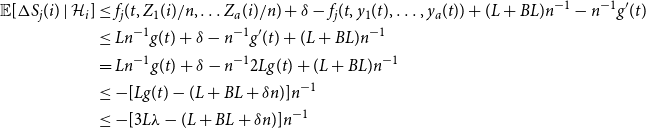 \begin{align} \mathbb {E}[\Delta S_j(i) \mid {\mathcal {H}}_i] & \le f_j(t, Z_1(i)/n, \ldots Z_a(i)/n) + \delta - f_j(t, y_1(t), \ldots, y_a(t)) + (L+BL)n^{-1} - n^{-1} g^{\prime}(t)\nonumber \\ & \le L n^{-1}g(t) + \delta - n^{-1} g^{\prime}(t) +(L+BL)n^{-1}\nonumber \\ & = L n^{-1}g(t) + \delta - n^{-1} 2L g(t) +(L+BL)n^{-1}\nonumber \\ & \le -[L g(t) - (L+BL + \delta n)]n^{-1}\nonumber \\ & \le -[3L \lambda - (L+BL + \delta n)]n^{-1} \\[-6pt] \nonumber \end{align}
 \begin{align} & \le 0, \\[12pt] \nonumber \end{align}
where the final line follows since
 $\lambda \ge \frac {L+BL + \delta n}{3L}$
.
$\lambda \ge \frac {L+BL + \delta n}{3L}$
.
Therefore, for
 $i^{\prime\prime} \le i \le i^{\prime}-1$
, we have that
$i^{\prime\prime} \le i \le i^{\prime}-1$
, we have that
 \begin{equation*} 0 \ge \mathbb {E}[\Delta S_j(i) \mid {\mathcal {H}}_i] = \mathbb {E}[\Delta X_j(i) \mid {\mathcal {H}}_i] + \mathbb {E}[\Delta M_j(i) \mid {\mathcal {H}}_i] = \Delta X_j(i) \end{equation*}
since
 $(M_j(i))_{i= 0}^{m}$
is a martingale and
$(M_j(i))_{i= 0}^{m}$
is a martingale and
 $\Delta X_j(i)$
is
$\Delta X_j(i)$
is
 ${\mathcal {H}}_{i}$
-measurable. In particular,
${\mathcal {H}}_{i}$
-measurable. In particular,
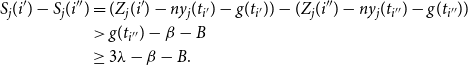
 \begin{equation} X_j(i^{\prime}) \le X_j(i^{\prime\prime}). \end{equation}
At this point, we use the event we assumed regarding
 $(M_{j}(i))_{i=0}^{m}$
(directly following (11)) to get that
$(M_{j}(i))_{i=0}^{m}$
(directly following (11)) to get that
 \begin{equation} M_j(i^{\prime}) - M_j(i^{\prime\prime}) \le |M_j(i^{\prime}) - M_j(0)| + |M_j(i^{\prime\prime}) - M_j(0)| \le 2\lambda . \end{equation}
But now we can derive our final contradiction (explanation follows):
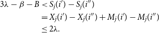 \begin{align*} 3 \lambda -\beta -B & \lt S_j(i^{\prime}) - S_j(i^{\prime\prime}) \\ &= X_j(i^{\prime}) - X_j(i^{\prime\prime}) + M_j(i^{\prime}) - M_j(i^{\prime\prime}) \\ & \le 2 \lambda . \end{align*}
Indeed the first line is from (13), the second is from the Doob decomposition, and the last line follows from (20) and (21). However, the last line is a contradiction since we chose
 $\lambda \ge \beta +B$
.
$\lambda \ge \beta +B$
.
Remark 9. We can relax several of the Conditions (a)–(c) on the
 $f_j$
and Conditions 1 and 2 of Theorem 2, and the conclusion still holds (in particular, the proof we gave still goes through). We will list some possible relaxations below:
$f_j$
and Conditions 1 and 2 of Theorem 2, and the conclusion still holds (in particular, the proof we gave still goes through). We will list some possible relaxations below:
-
• Condition (a): We only use this condition on (15) and (17), and in both situations, we are applying it at points
$(t, z_1, \ldots, z_a)$
, which are very close to the trajectory. In particular, instead of assuming that
$f_j$
is
$L$
-Lipschitz on all of
$\mathcal {D}$
, it suffices to have that
$f_j$
is
$L$
-Lipschitz on the set of points
\begin{equation*} \mathcal {D}^*\,:\!=\, \Big \{ (t, z_1, \ldots, z_a) \in \mathbb {R}^{a+1}: 0 \le t \le \sigma, y_{j^{\prime}}(t) \le z_{j^{\prime}} \le y_{j^{\prime}}(t) + g(t) { for } 1 \le j^{\prime} \le a \Big \} \subseteq \mathcal {D}. \end{equation*}
-
• Condition (b): We only use this condition to conclude that the system (6) has a unique solution and that those solutions
$y_j$
are
$B$
-Lipschitz. So, instead of Condition (b), it suffices to just check directly that (6) has a unique solution that is
$B$
-Lipschitz. -
• Condition (c): We only use the cooperativity of the functions to get line (16). In this situation, for our point
$(t, z_1, \ldots, z_a)$
, some
$z_j$
is in its critical interval (and all the
$z_i$
are below their upper bounds). In particular, instead of assuming the full Condition (c), for (16) it suffices to have that
$f_j(t, z_1, \ldots z_a)$
is upper bounded bywhenever
\begin{equation*} f_j\left (t, \frac {ny_1(t)+g(t)}{n}, \ldots, \frac {ny_{j-1}(t)+g(t)}{n}, z_j, \frac {ny_{j+1}(t)+g(t)}{n}, \ldots, \frac {ny_a(t)+g(t)}{n}\right ) \end{equation*}
$z_{j^{\prime}} \le y_{j^{\prime}}(t) + g(t)/n$
for all
$j^{\prime}$
and
$z_{j} \ge y_j(t)$
.
-
• Condition 2: We only use this condition to get (14). In this situation, we have that one of the
$Z_j$
is in its critical interval (and all the
$Z_i$
are below their upper bounds). Instead of Condition 2, it suffices to have the following: for each
$1 \le j \le a$
. If
$Z_{j^{\prime}}(i) \le ny_{j^{\prime}}(i/n) + g(i/n)$
for all
$1 \le j^{\prime}\le a$
and
$Z_j \ge ny_j(i/n)$
, then
$(i/n, Z_1(i)/n, \ldots Z_a(i)/n) \in \mathcal {D}$
and
\begin{equation*}\mathbb {E}[ \Delta Z_j(i) \mid {\mathcal {H}}_i] \le f_j(i/n, Z_1(i)/n, \ldots Z_a(i)/n) + \delta .\end{equation*}


4. Recovering a version of Wormald’s theorem
In this section, we recover the standard (two-sided) differential equation method of Wormald [Reference Wormald14]. The statement resembles the recent version given by Warnke [Reference Warnke13] in the sense that it does not use any asymptotic notation and instead gives explicit bounds for error estimates and failure probabilities. Like Warnke’s proof, ours has a probabilistic part and a deterministic part. Our probabilistic part is much the same as Warnke’s in that we apply a deviation inequality (though we use Freedman’s theorem rather than the Azuma-Hoeffding inequality) to the martingale part of a Doob decomposition. That being said, the deterministic part of our argument is quite different than the deterministic part of Warnke’s argument. In fact, we were not able to adapt Warnke’s argument to the one-sided setting.
Given
 $a \in \mathbb {N}$
, suppose that
$a \in \mathbb {N}$
, suppose that
 $\mathcal {D} \subseteq \mathbb {R}^{a+1}$
is a bounded domain, and for
$\mathcal {D} \subseteq \mathbb {R}^{a+1}$
is a bounded domain, and for
 $1 \le j \le a$
, let
$1 \le j \le a$
, let
 $f_j: \mathcal {D} \rightarrow \mathbb {R}$
. We assume that the following hold for each
$f_j: \mathcal {D} \rightarrow \mathbb {R}$
. We assume that the following hold for each
 $j$
:
$j$
:
-
1.
$f_j$
is
$L$
-Lipschitz, and -
2.
$|f_j|\le B$
on
$\mathcal {D}$
.


Given
 $(0,{\tilde y}_1, \ldots, {\tilde y}_a) \in \mathcal {D}$
, assume that
$(0,{\tilde y}_1, \ldots, {\tilde y}_a) \in \mathcal {D}$
, assume that
 $y_1(t), \ldots, y_a(t)$
is the (unique) solution to the system
$y_1(t), \ldots, y_a(t)$
is the (unique) solution to the system
 \begin{equation*} y_j^{\prime}(t) = f_j(t, y_1(t), \ldots, y_a(t)), \qquad y_j(0)={\tilde y}_j. \end{equation*}
for all
 $t \in [0, \sigma ]$
where
$t \in [0, \sigma ]$
where
 $\sigma$
is a positive value. Note that unlike in Theorem3, we make a further assumption involving
$\sigma$
is a positive value. Note that unlike in Theorem3, we make a further assumption involving
 $\sigma$
below in Theorem10.
$\sigma$
below in Theorem10.
Theorem 10.
Suppose for each
 $1 \le j \le a$
, we have a sequence of random variables
$1 \le j \le a$
, we have a sequence of random variables
 $(Y_j(i))_{i= 0}^\infty$
, which is adapted to the filtration
$(Y_j(i))_{i= 0}^\infty$
, which is adapted to the filtration
 $({\mathcal {H}}_i)_{i=0}^\infty$
. Let
$({\mathcal {H}}_i)_{i=0}^\infty$
. Let
 $n \in \mathbb {N}$
, and
$n \in \mathbb {N}$
, and
 $\beta, b, \lambda, \delta \gt 0$
be any parameters such that
$\beta, b, \lambda, \delta \gt 0$
be any parameters such that
 $\lambda \ge \frac {L+BL + \delta n}{3L}$
. Moreover, assume that
$\lambda \ge \frac {L+BL + \delta n}{3L}$
. Moreover, assume that
 $\sigma \gt 0$
is any value such that
$\sigma \gt 0$
is any value such that
 $(t,y_1(t), \ldots, y_a(t))$
has
$(t,y_1(t), \ldots, y_a(t))$
has
 $\ell ^{\infty }$
-distance at least
$\ell ^{\infty }$
-distance at least
 $3 \lambda e^{2Lt}/n$
from the boundary of
$3 \lambda e^{2Lt}/n$
from the boundary of
 $\mathcal {D}$
for all
$\mathcal {D}$
for all
 $t \in [0, \sigma )$
. Given an arbitrary stopping time
$t \in [0, \sigma )$
. Given an arbitrary stopping time
 $I \ge 0$
adapted to
$I \ge 0$
adapted to
 $({\mathcal {H}}_i)_{i=0}^\infty$
, suppose that the following properties hold for each
$({\mathcal {H}}_i)_{i=0}^\infty$
, suppose that the following properties hold for each
 $ 0 \le i \lt \min \{I, \sigma n \}$
:
$ 0 \le i \lt \min \{I, \sigma n \}$
:
-
1. The ‘Boundedness Hypothesis’:
$\max _{j} |\Delta Y_j(i)| \le \beta$
, and
$\max _{j} \mathbb {E}[ ( \Delta Y_{j}(i) )^2 \mid \mathcal {H}_i] \le b$
. -
2. The ‘Trend Hypothesis’: If
$(i/n, Y_1(i)/n, \ldots Y_a(i)/n) \in \mathcal {D}$
, then
for each
\begin{equation*}\Big |\mathbb {E}[ \Delta Y_j(i) \mid {\mathcal {H}}_i] - f_j(i/n, Y_1(i)/n, \ldots Y_a(i)/n)\Big | \le \delta \end{equation*}
$1 \le j \le a$
.
-
3. The ‘Initial Condition’:
$|Y_j(0) - y_j(0) n| \le \lambda$
for all
$1 \le j \le a$
.


Then, with probability at least
 $1 - 2 a \exp \left ( -\frac {\lambda ^2}{2( b \sigma n + 2\beta \lambda )} \right )$
,
$1 - 2 a \exp \left ( -\frac {\lambda ^2}{2( b \sigma n + 2\beta \lambda )} \right )$
,
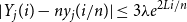 \begin{equation*} |Y_j(i) - ny_{j}(i/n)| \le 3 \lambda e^{2L i/n} \end{equation*}
for all
 $1 \le j \le a$
and
$1 \le j \le a$
and
 $0 \le i \le \min \{I, \sigma n\}$
.
$0 \le i \le \min \{I, \sigma n\}$
.
We conclude the section with an extension of Theorem10 analogous to Corollary7 of Theorem3. We omit the proof, as it follows almost identically to the proof of Corollary7.
Corollary 11 (of Theorem10). Suppose that in the terminology of Theorem 10, Conditions
1
and
2
are only verified for each
 $0 \le i \le \min \{I, \sigma n\}$
, which satisfies
$0 \le i \le \min \{I, \sigma n\}$
, which satisfies
 $|Y_{j^{\prime}}(i) - ny_{j^{\prime}}(i/n)| \le 3 \lambda e^{2Li/n}$
for all
$|Y_{j^{\prime}}(i) - ny_{j^{\prime}}(i/n)| \le 3 \lambda e^{2Li/n}$
for all
 $1 \le j^{\prime}\le a$
. In this case, the conclusion of Theorem 10 still holds. That is, with probability at least
$1 \le j^{\prime}\le a$
. In this case, the conclusion of Theorem 10 still holds. That is, with probability at least
 $1 - 2 a \exp \left ( -\frac {\lambda ^2}{2( b \sigma n + 2\beta \lambda )} \right )$
,
$1 - 2 a \exp \left ( -\frac {\lambda ^2}{2( b \sigma n + 2\beta \lambda )} \right )$
,
 \begin{equation*} |Y_j(i) - ny_{j}(i/n)| \le 3 \lambda e^{2L i/n} \end{equation*}
for all
 $1 \le j \le a$
and
$1 \le j \le a$
and
 $0 \le i \le \min \{I, \sigma n\}$
.
$0 \le i \le \min \{I, \sigma n\}$
.
Proof of Theorem
10
. Fix
 $0 \le i \le \sigma n$
, and again set
$0 \le i \le \sigma n$
, and again set
 $m\,:\!=\, \sigma n$
,
$m\,:\!=\, \sigma n$
,
 $t=t_i=i/n$
, and
$t=t_i=i/n$
, and
 $g(t)\,:\!=\, 3\lambda e^{2Lt}$
for convenience. Define
$g(t)\,:\!=\, 3\lambda e^{2Lt}$
for convenience. Define
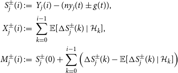 \begin{align*} S^{\pm }_j(i)&\,:\!=\,Y_j(i)-(ny_j(t) \pm g(t)),\\ X^{\pm }_j(i)&\,:\!=\,\sum _{k=0}^{i-1} \mathbb {E}[\Delta S^{\pm }_j(k) \mid {\mathcal {H}}_{k}],\\ M^{\pm }_j(i)&\,:\!=\, S^{\pm }_j(0) + \sum _{k=0}^{i-1} \left (\Delta S^{\pm }_j(k)- \mathbb {E}[\Delta S^{\pm }_j(k) \mid {\mathcal {H}}_{k}]\right ) \end{align*}
so that
 $(X^{\pm }_j(i) + M^{\pm }_j(i))_{i= 0}^{m}$
is the Doob decomposition of
$(X^{\pm }_j(i) + M^{\pm }_j(i))_{i= 0}^{m}$
is the Doob decomposition of
 $(S^{\pm }_j(i))_{i= 0}^m$
. Note that
$(S^{\pm }_j(i))_{i= 0}^m$
. Note that
 \begin{equation*} \Delta S^{\pm }_j(k)- \mathbb {E}[\Delta S^{\pm }_j(k) \mid {\mathcal {H}}_{k}] = \Delta Y_j(k)- \mathbb {E}[\Delta Y_j(k) \mid {\mathcal {H}}_{k}], \end{equation*}
and so
 $M^+_j(i)$
is almost the same as
$M^+_j(i)$
is almost the same as
 $M^-_j(i)$
. More precisely, we have
$M^-_j(i)$
. More precisely, we have
 \begin{equation*} M^{\pm }_j(i) = M_j(i) \mp g(0) \end{equation*}
where
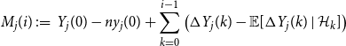 \begin{equation*} M_j(i)\,:\!=\, Y_j(0)-ny_j(0) + \sum _{k=0}^{i-1} \left (\Delta Y_j(k)- \mathbb {E}[\Delta Y_j(k) \mid {\mathcal {H}}_{k}]\right ) \end{equation*}
(which is also a martingale). As in the proof of Theorem3, we have
 $|\Delta M_j(i)| \le 2\beta$
and
$|\Delta M_j(i)| \le 2\beta$
and
 ${\textbf { Var}}[ \Delta M_{j}(i) \mid \mathcal {H}_i] \le b$
. Now, by Theorem8, we have that
${\textbf { Var}}[ \Delta M_{j}(i) \mid \mathcal {H}_i] \le b$
. Now, by Theorem8, we have that
 \begin{equation} \mathbb {P}\left (\exists \; 0 \le j \le a, 0 \le i \le m \mbox { such that } |M_j(i) - M_j(0)| \ge \lambda \right ) \le 2 a \exp \left ( -\frac {\lambda ^2}{2( b m + 2\beta \lambda )} \right ). \end{equation}
Suppose that the event above does not happen, so for all
 $0 \le j \le a,0 \le i \le m$
, we have that
$0 \le j \le a,0 \le i \le m$
, we have that
 $|M_j(i) - M_j(0)| \lt \lambda$
. We will show that we also have
$|M_j(i) - M_j(0)| \lt \lambda$
. We will show that we also have
 $|Y_j(i) - ny_j(t)|\le g(t)$
for all
$|Y_j(i) - ny_j(t)|\le g(t)$
for all
 $0 \le i \le m$
. Note that
$0 \le i \le m$
. Note that
 $y_j$
is
$y_j$
is
 $B$
-Lipschitz as before. Define the critical interval
$B$
-Lipschitz as before. Define the critical interval
 \begin{equation*} I_j(i) \,:\!=\, \left [ ny_j(t)-g(t), ny_j(t)+g(t)\right ]. \end{equation*}
Suppose for the sake of contradiction that
 $i^{\prime}$
is minimal with
$i^{\prime}$
is minimal with
 $0 \le i^{\prime} \le m$
and
$0 \le i^{\prime} \le m$
and
 $Y_j(i^{\prime}) \notin I_j(i^{\prime})$
for some
$Y_j(i^{\prime}) \notin I_j(i^{\prime})$
for some
 $j$
. We will consider the case where
$j$
. We will consider the case where
 $Y_j(i^{\prime}) \gt ny_j(t)+g(t)$
(the case where
$Y_j(i^{\prime}) \gt ny_j(t)+g(t)$
(the case where
 $Y_j(i^{\prime}) \lt ny_j(t)-g(t)$
is handled similarly with some inequalities reversed). In other words,
$Y_j(i^{\prime}) \lt ny_j(t)-g(t)$
is handled similarly with some inequalities reversed). In other words,
 $S^+_j(i^{\prime}) \gt 0$
. First observe that since
$S^+_j(i^{\prime}) \gt 0$
. First observe that since
 $g(0)\,:\!=\,3 \lambda$
, Condition 3 implies
$g(0)\,:\!=\,3 \lambda$
, Condition 3 implies
 $S^+_j(0) \le -2\lambda$
. In particular,
$S^+_j(0) \le -2\lambda$
. In particular,
 $i^{\prime} \gt 0$
and
$i^{\prime} \gt 0$
and
 \begin{equation} S^+_j(i^{\prime}) - S^+_j(0) \gt 2\lambda . \end{equation}
For
 $0\le i \lt i^{\prime}$
, we have (explanation follows)
$0\le i \lt i^{\prime}$
, we have (explanation follows)
 \begin{align*} \mathbb {E}[\Delta S^+_{j}(i) \mid {\mathcal {H}}_i] & = \mathbb {E}[ \Delta Y_{j}(i) \mid {\mathcal {H}}_i] - \Delta ny_j(t) - \Delta g(t)\\ & \le f_j(t, Y_1(i)/n, \ldots Y_a(i)/n) + \delta - f_j(t, y_1(t), \ldots, y_a(t)) + (L+BL)n^{-1} - n^{-1} g^{\prime}(t)\\ & \le Ln^{-1}g(t) + \delta +(L+BL)n^{-1} - n^{-1} g^{\prime}(t)\\ & \le -[3L \lambda - (L+BL + \delta n)]n^{-1}\\ & \le 0. \end{align*}
Indeed, the first line is by definition, and the second line follows just like (14), with the minor caveat that we now must show that
 $(t, Y_1(i)/n, \ldots, Y_a(i)/n)$
is within the domain
$(t, Y_1(i)/n, \ldots, Y_a(i)/n)$
is within the domain
 $\mathcal {D}$
to apply Condition 2 (recall that in Theorem3, this is simply assumed). Observe that by the definition of
$\mathcal {D}$
to apply Condition 2 (recall that in Theorem3, this is simply assumed). Observe that by the definition of
 $\sigma$
,
$\sigma$
,
 $(t, y_1(t), \ldots, y_{a}(t))$
is in
$(t, y_1(t), \ldots, y_{a}(t))$
is in
 $\mathcal {D}$
and at least
$\mathcal {D}$
and at least
 $\ell ^{\infty }$
-distance
$\ell ^{\infty }$
-distance
 $g(t)/n$
from the boundary of
$g(t)/n$
from the boundary of
 $\mathcal {D}$
. On the other hand, since
$\mathcal {D}$
. On the other hand, since
 $Y_{j^{\prime}}(i) \in I_{j^{\prime}}(i)$
for all
$Y_{j^{\prime}}(i) \in I_{j^{\prime}}(i)$
for all
 $1 \le j^{\prime} \le a$
, we know that
$1 \le j^{\prime} \le a$
, we know that
 $|Y_{j^{\prime}}(i)/n - y_{j^{\prime}}(t)| \le g(t)/n$
for all
$|Y_{j^{\prime}}(i)/n - y_{j^{\prime}}(t)| \le g(t)/n$
for all
 $1 \le j^{\prime} \le a$
. Thus,
$1 \le j^{\prime} \le a$
. Thus,
 $(t, Y_1(i)/n, \ldots Y_a(i)/n) \in \mathcal {D}$
, and so
$(t, Y_1(i)/n, \ldots Y_a(i)/n) \in \mathcal {D}$
, and so
 \begin{equation*}\mathbb {E}[ \Delta Y_{j}(i) \mid {\mathcal {H}}_i] \le f_j(t, Y_1(i)/n, \ldots, Y_a(i)/n) + \delta \end{equation*}
by Condition 2. The remaining justification is much the same as before. Since
 $f_j$
is
$f_j$
is
 $L$
-Lipschitz and
$L$
-Lipschitz and
 $|Y_{j^{\prime}}(i) - ny_{j^{\prime}}(t)|\le g(t)$
for all
$|Y_{j^{\prime}}(i) - ny_{j^{\prime}}(t)|\le g(t)$
for all
 $j^{\prime}$
, we have
$j^{\prime}$
, we have
 $f_j(t, Y_1(i)/n, \ldots Y_a(i)/n) \le f_j(t, y_1(t), \ldots, y_a(t))+Ln^{-1}g(t)$
, and the third line follows. The fourth and fifth lines follow just as (18) and (19). Therefore, for
$f_j(t, Y_1(i)/n, \ldots Y_a(i)/n) \le f_j(t, y_1(t), \ldots, y_a(t))+Ln^{-1}g(t)$
, and the third line follows. The fourth and fifth lines follow just as (18) and (19). Therefore, for
 $0 \le i \lt i^{\prime}$
, we have that
$0 \le i \lt i^{\prime}$
, we have that
 \begin{equation*} 0 \ge \mathbb {E}[\Delta S^+_j(i) \mid {\mathcal {H}}_i] = \mathbb {E}[\Delta X^+_j(i) \mid {\mathcal {H}}_i] + \mathbb {E}[\Delta M^+_j(i) \mid {\mathcal {H}}_i] = \Delta X^+_j(i) \end{equation*}
since
 $(M^+_j(i))_{i= 0}^\infty$
is a martingale and
$(M^+_j(i))_{i= 0}^\infty$
is a martingale and
 $\Delta X^+_j(i)$
is
$\Delta X^+_j(i)$
is
 ${\mathcal {H}}_{i}$
-measurable. In particular
${\mathcal {H}}_{i}$
-measurable. In particular
 \begin{equation} X^+_j(i^{\prime}) \le X^+_j(0). \end{equation}
But now, we can derive our final contradiction (explanation follows):
 \begin{align*} 2 \lambda &\lt S^+_j(i^{\prime}) - S^+_j(0) \\ & = X^+_j(i^{\prime}) - X^+_j(0) + M_j(i^{\prime}) - M_j(0)\\ &\le \lambda . \end{align*}
Indeed, the first line is from (23), the second line is from the Doob decomposition, and the last follows from (24), and our assumption is that the event described in line (22) does not happen. Of course,
 $2\lambda \lt \lambda$
is a contradiction, and we are done.
$2\lambda \lt \lambda$
is a contradiction, and we are done.
Acknowledgements
Supported in part by Simons Foundation Grant #848648. The majority of the author’s work done on this paper was while they were affiliated with the Department of Computer Science at the University of Toronto.
