


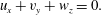
1 Introduction
Several investigations of model jet problems such as round or planar jets have repeatedly shown the appearance of coherent vortical structures in the flow. When fluid is injected from a round jet nozzle into an open ambient region, the mixing layer emanating from the lip of the jet nozzle produces coherent ring vortices. The mixing layer then grows downstream, and eventually a self-similar mean flow is developed. Jung, Gamard & George (Reference Jung, Gamard and George2004) showed that the streamwise evolution of the coherent structure changes from initially axisymmetric vortices to a helical structure with maximum energy associated with azimuthal mode number
 $m=2$
. Subsequently Iqbal & Thomas (Reference Iqbal and Thomas2007) showed that helical mode
$m=2$
. Subsequently Iqbal & Thomas (Reference Iqbal and Thomas2007) showed that helical mode
 $m=1$
eventually grows to dominate. The locally parallel linear stability analysis using the local mean velocity profile as the background flow indeed predicts the dominance of helical mode
$m=1$
eventually grows to dominate. The locally parallel linear stability analysis using the local mean velocity profile as the background flow indeed predicts the dominance of helical mode
 $m=1$
. The development of the streaky field has also been studied in relation to the effect of nozzle jet. As shown in Liepmann & Morteza (Reference Liepmann and Morteza1992), and in the more recent review paper by Ball, Fellouah & Pollard (Reference Ball, Fellouah and Pollard2012), the instability of the mixing layer produces the streamwise vorticity in the initial development of the jet, which results from nonlinear roll-up of the vortex sheet. While the turbulent round jet flow is dominated by the helical inviscid instability mentioned above, there are various smaller-scale vortical structures induced in the flow. Such short-scale vortices may also have an ability to modify the streaky field. However, to the best of the authors’ knowledge, no self-consistent theoretical description of that feedback effect is yet available.
$m=1$
. The development of the streaky field has also been studied in relation to the effect of nozzle jet. As shown in Liepmann & Morteza (Reference Liepmann and Morteza1992), and in the more recent review paper by Ball, Fellouah & Pollard (Reference Ball, Fellouah and Pollard2012), the instability of the mixing layer produces the streamwise vorticity in the initial development of the jet, which results from nonlinear roll-up of the vortex sheet. While the turbulent round jet flow is dominated by the helical inviscid instability mentioned above, there are various smaller-scale vortical structures induced in the flow. Such short-scale vortices may also have an ability to modify the streaky field. However, to the best of the authors’ knowledge, no self-consistent theoretical description of that feedback effect is yet available.
For simplicity in theoretical and computational studies planar jets have usually been used; see, for example, Bickley (Reference Bickley1937), Tatsumi & Kakutani (Reference Tatsumi and Kakutani1958), Howard (Reference Howard1959), Clenshaw & Elliott (Reference Clenshaw and Elliott1960). The scenario described above for round jets is also valid for planar flows (see Kozlov et al. (Reference Kozlov, Grek, Löfdahl, Chernorai and Litvinenko2002) for example), and the mechanism by which the streaky structures are initiated is of great concern. The experimental study of the planar jet flow has also been an active area of research dating back to Schlichting (Reference Schlichting1933); see also Sato (Reference Sato1960), Gutmark & Wygnanski (Reference Gutmark and Wygnanski1976), Thomas & Chu (Reference Thomas and Chu1989), Deo, Mi & Nathan (Reference Deo, Mi and Nathan2008). Lambda vortices are typical small-scale coherent structures observed in various shear flows. Recently, Sakakibara & Anzai (Reference Sakakibara and Anzai2001) showed that lambda shape vortices naturally develop in controlled planar jet experiments and confirmed that the vortices persist for a rather long streamwise distance.
Jet flows involve extraordinarily complicated coherent vortices of various scales because of their downstream evolution. Therefore, reduction of the flow dynamics has often been carried out. For example Gordeyev & Thomas (Reference Gordeyev and Thomas2000, Reference Gordeyev and Thomas2002), Gamard, Jung & George (Reference Gamard, Jung and George2004) and Jung et al. (Reference Jung, Gamard and George2004) used proper orthogonal decomposition to reduce the dynamical systems to lower dimensions, whilst Le Ribault, Sarkar & Stanley (Reference Le Ribault, Sarkar and Stanley1999) and Fureby & Grinstein (Reference Fureby and Grinstein2002) used large eddy simulations to reduce the computational cost. While the above empirically derived modified descriptions of the governing equations or the reduced description of the experimental or numerical results are useful in practice, they are not based on rational theoretical considerations of the Navier–Stokes equations.
Our aim in this paper is to construct rational approximations to the nonlinear states for a planar jet using a large-Reynolds-number matched asymptotic expansion procedure. Unlike the fully computational approach, which becomes progressively more computationally demanding as the Reynolds number increases, in our reduced model the Reynolds number is scaled out of the problem. Once a consistent asymptotic expansion is found, it is straightforward to derive the reduced equations, without any artificial assumptions. The solution of the reduced equations completely determines the coefficients in the leading-order asymptotic expansions that can be used to predict the behaviour of Navier–Stokes solutions.
In order to simplify the problem as much as possible, we restrict our attention to time-periodic flows. In recent years there has been much interest in the description of nonlinear periodic states in simple shear flows such as plane Couette flow; see the review paper by Kawahara, Uhlmann & van Veen (Reference Kawahara, Uhlmann and van Veen2012). The nonlinear periodic solutions, also referred to as ‘exact coherent structures’, found in shear flows are often weakly unstable, in the sense that they only have a few unstable eigenvalues. Therefore results from dynamical systems theory applied to turbulence suggest that turbulent trajectories in phase space would tend to stay for a long time around the solutions before eventually moving away. Therefore, unstable periodic solutions can be regarded as skeletons on which the chaotic dynamics of developed turbulence or transition to turbulence hangs. Usually solutions found for parallel shear flows have been captured by directly applying a Newton method to the discretised Navier–Stokes equations; see Nagata (Reference Nagata1990), Clever & Busse (Reference Clever and Busse1992), Kawahara & Kida (Reference Kawahara and Kida2001), Waleffe (Reference Waleffe2001).
We are concerned with the nonlinear interaction of small-scale lambda vortices and the globally induced streaky field. The asymptotic theory on which our solution is based was first developed by Deguchi & Hall (Reference Deguchi and Hall2014a ). In that work the asymptotic suction boundary layer (ASBL) was investigated. ASBL is a well-known canonical boundary layer flow where the development of the boundary layer growth is suppressed by a uniform vertical suction on the wall. Since the flow is parallel, a full Navier–Stokes-based computational approach can also be used to find coherent structures. By solving for nonlinear states using Newton’s method, two types of travelling wave solutions have been found. The first one produces near-wall vortices governed by the vortex–wave interaction theory of Hall & Smith (Reference Hall and Smith1991) and Hall & Sherwin (Reference Hall and Sherwin2010), whilst here our focus is on the second ‘free-stream coherent structure’ type that has coherent vortices interacting in a layer near the free stream of the boundary layer. Both of the asymptotic theories were found to be in excellent agreement with full numerical solutions.
In the layer where free-stream coherent structures are generated the flow satisfies a canonical nonlinear eigenvalue problem associated with the Navier–Stokes equations at unit Reynolds number; surprisingly it turns out that the problem is generic to a wide range of flows. For example, Deguchi & Hall (Reference Deguchi and Hall2014b ) investigated the Burgers vortex sheet and showed that the theory can be used to describe nonlinear structures associated with the vortex sheet. Subsequently, Deguchi & Hall (Reference Deguchi and Hall2015a ) extended the theory to quite general two-dimensional boundary layers over flat plates, and accounted for non-parallel effects.
However, here we will show that the extension of the theory to jet problems is not a trivial task. We begin the analysis by formulating the problem in the next section. In the same section we shall also highlight the differences between the present problem and our previous work. In § 3 we shall perform a mathematical analysis and numerical computations to construct the asymptotic solution based on a large-Reynolds-number assumption. Finally, in § 4, we shall discuss implications of our analysis.
2 Formulation of the problem
Consider a free planar jet where an incompressible Newtonian fluid is injected from a steady source at the origin of Cartesian coordinate
 $(x^{\ast },y^{\ast },z^{\ast })$
. We take
$(x^{\ast },y^{\ast },z^{\ast })$
. We take
 $x^{\ast }$
to be in the streamwise direction and assume that the injection is uniform in the spanwise direction
$x^{\ast }$
to be in the streamwise direction and assume that the injection is uniform in the spanwise direction
 $z^{\ast }$
. The
$z^{\ast }$
. The
 $y^{\ast }$
direction is referred to as the vertical direction. The Reynolds number is defined using a typical fluid velocity
$y^{\ast }$
direction is referred to as the vertical direction. The Reynolds number is defined using a typical fluid velocity
 $U^{\ast }$
, a typical streamwise length scale
$U^{\ast }$
, a typical streamwise length scale
 $L^{\ast }$
, and the kinematic viscosity of the fluid
$L^{\ast }$
, and the kinematic viscosity of the fluid
 $\unicode[STIX]{x1D708}$
. If the Reynolds number
$\unicode[STIX]{x1D708}$
. If the Reynolds number
 $R=U^{\ast }L^{\ast }/\unicode[STIX]{x1D708}$
is large, the vertical thickness of the jet is much smaller than
$R=U^{\ast }L^{\ast }/\unicode[STIX]{x1D708}$
is large, the vertical thickness of the jet is much smaller than
 $L^{\ast }$
. The usual boundary layer scaling argument predicts the thickness normalised by
$L^{\ast }$
. The usual boundary layer scaling argument predicts the thickness normalised by
 $L^{\ast }$
is proportional to
$L^{\ast }$
is proportional to
 $\unicode[STIX]{x1D6FF}\equiv R^{-1/2}$
. Normalising the spatial variables and velocities as
$\unicode[STIX]{x1D6FF}\equiv R^{-1/2}$
. Normalising the spatial variables and velocities as
 $(x,y,z)=(x^{\ast },\unicode[STIX]{x1D6FF}^{-1}y^{\ast },\unicode[STIX]{x1D6FF}^{-1}z^{\ast })/L^{\ast }$
,
$(x,y,z)=(x^{\ast },\unicode[STIX]{x1D6FF}^{-1}y^{\ast },\unicode[STIX]{x1D6FF}^{-1}z^{\ast })/L^{\ast }$
,
 $(u,v,w)=(u^{\ast },\unicode[STIX]{x1D6FF}^{-1}v^{\ast },\unicode[STIX]{x1D6FF}^{-1}w^{\ast })/U^{\ast }$
, the flow is governed by the non-dimensional Navier–Stokes equations
$(u,v,w)=(u^{\ast },\unicode[STIX]{x1D6FF}^{-1}v^{\ast },\unicode[STIX]{x1D6FF}^{-1}w^{\ast })/U^{\ast }$
, the flow is governed by the non-dimensional Navier–Stokes equations
 $$\begin{eqnarray}\displaystyle & \displaystyle (\unicode[STIX]{x2202}_{t}+\boldsymbol{u}\boldsymbol{\cdot }\unicode[STIX]{x1D735})u=-R^{-1}p_{x}+R^{-1}u_{xx}+u_{yy}+u_{zz}, & \displaystyle\end{eqnarray}$$
 $$\begin{eqnarray}\displaystyle & \displaystyle (\unicode[STIX]{x2202}_{t}+\boldsymbol{u}\boldsymbol{\cdot }\unicode[STIX]{x1D735})v=-p_{y}+R^{-1}v_{xx}+v_{yy}+v_{zz}, & \displaystyle\end{eqnarray}$$
 $$\begin{eqnarray}\displaystyle & \displaystyle (\unicode[STIX]{x2202}_{t}+\boldsymbol{u}\boldsymbol{\cdot }\unicode[STIX]{x1D735})w=-p_{z}+R^{-1}w_{xx}+w_{yy}+w_{zz}, & \displaystyle\end{eqnarray}$$
 $$\begin{eqnarray}\displaystyle & \displaystyle u_{x}+v_{y}+w_{z}=0. & \displaystyle\end{eqnarray}$$
 $p$
and time
$p$
and time
 $t$
are normalised by
$t$
are normalised by
 $\unicode[STIX]{x1D70C}U^{\ast 2}$
and
$\unicode[STIX]{x1D70C}U^{\ast 2}$
and
 $L^{\ast }/U^{\ast }$
, respectively, using the fluid density
$L^{\ast }/U^{\ast }$
, respectively, using the fluid density
 $\unicode[STIX]{x1D70C}$
. Throughout the paper we assume that the flow is symmetric in
$\unicode[STIX]{x1D70C}$
. Throughout the paper we assume that the flow is symmetric in
 $y$
. We also assume that the velocity vanishes for large
$y$
. We also assume that the velocity vanishes for large
 $y$
and that the flow is periodic in
$y$
and that the flow is periodic in
 $z$
with wavenumber
$z$
with wavenumber
 $\unicode[STIX]{x1D6FD}_{0}$
.
$\unicode[STIX]{x1D6FD}_{0}$
. In the large-
 $R$
limit, the basic two-dimensional flow satisfies Prandtl’s boundary layer equations with zero-pressure gradient. For the jet problem, there is the well-known self-similar solution (see Bickley Reference Bickley1937; Schlichting Reference Schlichting1979, for example):
$R$
limit, the basic two-dimensional flow satisfies Prandtl’s boundary layer equations with zero-pressure gradient. For the jet problem, there is the well-known self-similar solution (see Bickley Reference Bickley1937; Schlichting Reference Schlichting1979, for example):
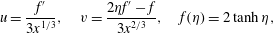 $$\begin{eqnarray}\displaystyle u=\frac{f^{\prime }}{3x^{1/3}},\quad v=\frac{2\unicode[STIX]{x1D702}f^{\prime }-f}{3x^{2/3}},\quad f(\unicode[STIX]{x1D702})=2\tanh \unicode[STIX]{x1D702}, & & \displaystyle\end{eqnarray}$$
where
 $\unicode[STIX]{x1D702}$
is the similarity variable
$\unicode[STIX]{x1D702}$
is the similarity variable
 $\unicode[STIX]{x1D702}=yx^{-2/3}/3$
. Here the momentum flux
$\unicode[STIX]{x1D702}=yx^{-2/3}/3$
. Here the momentum flux
 $\int _{-\infty }^{\infty }u^{2}\,\text{d}y$
is a conserved quantity and, without any loss of generality, we can choose it to be
$\int _{-\infty }^{\infty }u^{2}\,\text{d}y$
is a conserved quantity and, without any loss of generality, we can choose it to be
 $16/27$
. A sketch of the basic flow profile is shown in figure 1.
$16/27$
. A sketch of the basic flow profile is shown in figure 1.
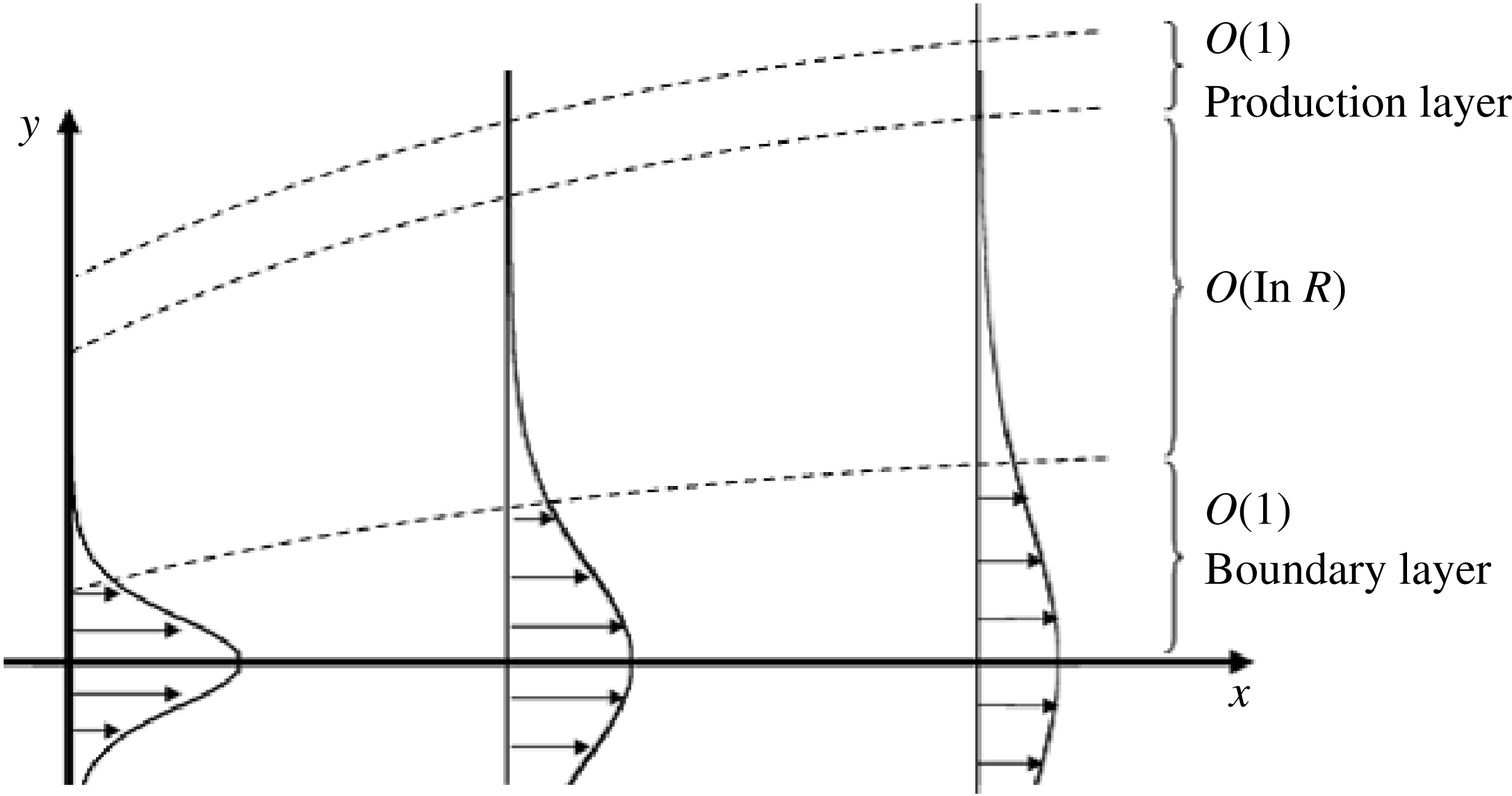
Figure 1. Schematic of the basic self-similar planar jet flow and the asymptotic regions concerned in this paper. The arrows indicate the streamwise basic flow profile. The basic flow develops a thin boundary layer structure near the centre of the jet. However, it should be noted in the figure that the thickness of that layer is
 $O(1)$
in our non-dimensional coordinate as we have used boundary layer scaling. The production layer is the position where the basic flow advection is comparable to the viscous effect, and wave-like coherent structures are produced. The thickness of the production layer is the same as that for the boundary layer.
$O(1)$
in our non-dimensional coordinate as we have used boundary layer scaling. The production layer is the position where the basic flow advection is comparable to the viscous effect, and wave-like coherent structures are produced. The thickness of the production layer is the same as that for the boundary layer.
Table 1. Summary of the flows relevant to free-stream coherent structures theory for ASBL (Deguchi & Hall Reference Deguchi and Hall2014a ), the Burgers vortex sheet (Deguchi & Hall Reference Deguchi and Hall2014b ), two-dimensional boundary layers (Deguchi & Hall Reference Deguchi and Hall2015a ), and planar jets (this study).
3 The asymptotic description of coherent structures in jets
3.1 Outline of the asymptotic theory
In this section we seek a time-periodic solution of (2.1) with fixed frequency
 $\unicode[STIX]{x1D6FA}_{0}$
using a large-Reynolds-number asymptotic approach. The overall asymptotic structure is similar to that found for ASBL by Deguchi & Hall (Reference Deguchi and Hall2014a
); namely we assume that wave-like coherent structures are produced in a ‘production layer’ located a distance
$\unicode[STIX]{x1D6FA}_{0}$
using a large-Reynolds-number asymptotic approach. The overall asymptotic structure is similar to that found for ASBL by Deguchi & Hall (Reference Deguchi and Hall2014a
); namely we assume that wave-like coherent structures are produced in a ‘production layer’ located a distance
 $O(\ln R)$
from the centre of the jet. A sketch of the different asymptotic regions is given in figure 1. We denote the basic planar shear flow as
$O(\ln R)$
from the centre of the jet. A sketch of the different asymptotic regions is given in figure 1. We denote the basic planar shear flow as
 $u_{b},v_{b}$
, where the leading-order part is given by (2.2). The key step in finding the location of the production layer is the far-field form of the basic flow:
$u_{b},v_{b}$
, where the leading-order part is given by (2.2). The key step in finding the location of the production layer is the far-field form of the basic flow:
 $$\begin{eqnarray}\displaystyle u_{b}\rightarrow FG\text{e}^{-2\unicode[STIX]{x1D702}},\quad v_{b}\rightarrow -F,\quad \text{as}~\unicode[STIX]{x1D702}\rightarrow \infty , & & \displaystyle\end{eqnarray}$$
where
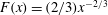 $F(x)=(2/3)x^{-2/3}$
,
$F(x)=(2/3)x^{-2/3}$
,
 $G(x)=4x^{1/3}$
. An important point to note here is that the streamwise component approaches a free-stream speed exponentially as is the case for ASBL, and the effective Reynolds number becomes small in the far field. In the production layer, the flow is governed by the Navier–Stokes equations with an effective Reynolds number of unity, and thus wave-like free-stream coherent structures can be generated. The position of the layer can easily be found by a simple order-of-magnitude analysis. We first note that in order to recover the streamwise derivative in the right-hand side of (2.1), we must set
$G(x)=4x^{1/3}$
. An important point to note here is that the streamwise component approaches a free-stream speed exponentially as is the case for ASBL, and the effective Reynolds number becomes small in the far field. In the production layer, the flow is governed by the Navier–Stokes equations with an effective Reynolds number of unity, and thus wave-like free-stream coherent structures can be generated. The position of the layer can easily be found by a simple order-of-magnitude analysis. We first note that in order to recover the streamwise derivative in the right-hand side of (2.1), we must set
 $\unicode[STIX]{x2202}_{x}\sim O(R^{1/2})$
. Then for the convective term to balance with the viscous terms in the equations of motion we require
$\unicode[STIX]{x2202}_{x}\sim O(R^{1/2})$
. Then for the convective term to balance with the viscous terms in the equations of motion we require
 $\text{e}^{-2\unicode[STIX]{x1D702}}\unicode[STIX]{x2202}_{x}\sim O(R^{0})$
. Combining these balances, we have
$\text{e}^{-2\unicode[STIX]{x1D702}}\unicode[STIX]{x2202}_{x}\sim O(R^{0})$
. Combining these balances, we have
 $$\begin{eqnarray}\displaystyle \text{e}^{-2\unicode[STIX]{x1D702}}\sim O(R^{-1/2}), & & \displaystyle\end{eqnarray}$$
from which we find that the production layer is located at
 $\unicode[STIX]{x1D702}\sim O(\ln R)$
.
$\unicode[STIX]{x1D702}\sim O(\ln R)$
.
Of course, since the jet problem is non-parallel, the flow structure beneath the production layer is more complicated than is the case for ASBL. The free-stream coherent structures theory for the spatially growing problem was developed by Deguchi & Hall (Reference Deguchi and Hall2015a ) for a quite general class of two-dimensional boundary layers. However, for the reasons given below a direct application of that theory to the jet problem is not possible.
The first reason is that for the boundary layer flows the decay of the basic flow correction is Gaussian rather than exponential. As found earlier (Deguchi & Hall Reference Deguchi and Hall2014b
) for the Burgers vortex sheet, even for this case we can determine the location of the production layer because locally the behaviour of the basic flow correction is of exponential form in terms of a scaled variable. However, since the basic flow beneath the production layer is not of exponential form, the induced vortex structure there develops in a quite different way than was the case for ASBL. In the adjustment zone between the near-wall boundary layer and the production layer the vertical and spanwise scales are different. Surprisingly, that difference allows us to solve the adjustment problem analytically to find the maximum amplitude of the induced streak there. In contrast, for the jet problem the far-field approximation of the basic flow (3.1) is valid except for the boundary layer near the centre of the jet. This means that there is no need for an adjustment layer, and thus the streak beneath the production layer takes its maximum in the boundary layer as for the ASBL case. The non-parallel effect becomes evident in the boundary layer, because the natural streamwise scale of the flow here becomes
 $O(1)$
in
$O(1)$
in
 $x$
. The vertical and spanwise scales are comparable there, and we must therefore use a numerical approach.
$x$
. The vertical and spanwise scales are comparable there, and we must therefore use a numerical approach.
The second reason why the jet and growing boundary layer problems differ is the difference between the free-stream speeds in the jet and boundary layer problems. In order to construct a periodic solution in the production layer of non-parallel flows, we describe travelling wave states varying locally using a Wentzel–Kramers–Brillouin (WKB) method. The streamwise wavenumber of the local travelling wave must be chosen appropriately to construct the global solution. In the boundary layer problem, the local wavenumber can be simply fixed by the free-stream speed and the global frequency of the periodic solution. However, since for the jet problem the free-stream speed is zero, clearly the same technique cannot be used. Of course this problem is inherently associated with non-parallel effects. The analysis in the next section shows that the global frequency of the jet problem can be related to the phase speed of the local travelling waves, rather than the wavenumber.
3.2 Production layer analysis
Now let us derive the canonical problem that governs nonlinear free-stream coherent structures in the production layer. Following the discussion in the previous section, we define the scaled vertical coordinate
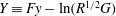 $Y\equiv Fy-\ln (R^{1/2}G)$
. Since
$Y\equiv Fy-\ln (R^{1/2}G)$
. Since
 $2\unicode[STIX]{x1D702}=Fy$
, the large-
$2\unicode[STIX]{x1D702}=Fy$
, the large-
 $\unicode[STIX]{x1D702}$
form of the basic flow (3.1) then becomes
$\unicode[STIX]{x1D702}$
form of the basic flow (3.1) then becomes
 $$\begin{eqnarray}\displaystyle u_{b}=R^{-1/2}F\text{e}^{-Y}+\cdots \,,\quad v_{b}=-F+\cdots \,. & & \displaystyle\end{eqnarray}$$
Beneath the production layer, we assume that the flow is simply the unperturbed jet flow to leading order with a small correction induced by the flow in the production layer.
In order to have a unit-Reynolds-number Navier–Stokes problem in the production layer, the scaled spanwise variable
 $Z=Fz$
is now introduced. In order to allow for a wave-like dependence of the flow in the streamwise direction, we introduce a WKB phase function
$Z=Fz$
is now introduced. In order to allow for a wave-like dependence of the flow in the streamwise direction, we introduce a WKB phase function
 $\unicode[STIX]{x1D6F7}\in [0,2\unicode[STIX]{x03C0}]$
defined by
$\unicode[STIX]{x1D6F7}\in [0,2\unicode[STIX]{x03C0}]$
defined by
 $$\begin{eqnarray}\displaystyle \unicode[STIX]{x1D6F7}=-R^{1/2}\left(\int ^{x}[F\unicode[STIX]{x1D6FC}_{0}(x)+\cdots \,]\,\text{d}x-R^{-1/2}\unicode[STIX]{x1D6FA}_{0}t\right), & & \displaystyle\end{eqnarray}$$
so that
 $\unicode[STIX]{x2202}_{x}=-R^{1/2}F\unicode[STIX]{x1D6FC}_{0}\unicode[STIX]{x2202}_{\unicode[STIX]{x1D6F7}}+\cdots \,$
. Here
$\unicode[STIX]{x2202}_{x}=-R^{1/2}F\unicode[STIX]{x1D6FC}_{0}\unicode[STIX]{x2202}_{\unicode[STIX]{x1D6F7}}+\cdots \,$
. Here
 $\unicode[STIX]{x1D6FC}_{0}$
is the local streamwise wavenumber of the travelling wave, and the minus sign has been introduced to aid comparison with Deguchi & Hall (Reference Deguchi and Hall2014a
). Note that
$\unicode[STIX]{x1D6FC}_{0}$
is the local streamwise wavenumber of the travelling wave, and the minus sign has been introduced to aid comparison with Deguchi & Hall (Reference Deguchi and Hall2014a
). Note that
 $\unicode[STIX]{x1D6FC}_{0}$
is real, and varies in the streamwise direction, whereas the frequency
$\unicode[STIX]{x1D6FC}_{0}$
is real, and varies in the streamwise direction, whereas the frequency
 $\unicode[STIX]{x1D6FA}_{0}$
is constant. We now substitute the expansions
$\unicode[STIX]{x1D6FA}_{0}$
is constant. We now substitute the expansions
 $$\begin{eqnarray}\displaystyle & \displaystyle u=-R^{-1/2}FU(\unicode[STIX]{x1D6F7},Y,Z)+\cdots \,,\quad v=FV(\unicode[STIX]{x1D6F7},Y,Z)+\cdots \,, & \displaystyle\end{eqnarray}$$
 $$\begin{eqnarray}\displaystyle & \displaystyle w=FW(\unicode[STIX]{x1D6F7},Y,Z)+\cdots \,,\quad p=F^{2}P(\unicode[STIX]{x1D6F7},Y,Z)+\cdots \,, & \displaystyle\end{eqnarray}$$
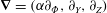
 $$\begin{eqnarray}\displaystyle \unicode[STIX]{x1D6FC}=\unicode[STIX]{x1D6FC}_{0},\quad \unicode[STIX]{x1D6FD}=\frac{\unicode[STIX]{x1D6FD}_{0}}{F},\quad c_{1}=\frac{\unicode[STIX]{x1D6FA}_{0}}{\unicode[STIX]{x1D6FC}_{0}F^{2}}. & & \displaystyle\end{eqnarray}$$
The leading-order problem then becomes
 $$\begin{eqnarray}\displaystyle ([\boldsymbol{U}+c_{1}\boldsymbol{i}]\boldsymbol{\cdot }\unicode[STIX]{x1D735})\boldsymbol{U}=-\unicode[STIX]{x1D735}P+\unicode[STIX]{x1D6FB}^{2}\boldsymbol{U},\quad \unicode[STIX]{x1D735}\boldsymbol{\cdot }\boldsymbol{U}=0, & & \displaystyle\end{eqnarray}$$
where
 $\unicode[STIX]{x1D735}=(\unicode[STIX]{x1D6FC}\unicode[STIX]{x2202}_{\unicode[STIX]{x1D6F7}},\unicode[STIX]{x2202}_{Y},\unicode[STIX]{x2202}_{Z})$
. Note here that
$\unicode[STIX]{x1D735}=(\unicode[STIX]{x1D6FC}\unicode[STIX]{x2202}_{\unicode[STIX]{x1D6F7}},\unicode[STIX]{x2202}_{Y},\unicode[STIX]{x2202}_{Z})$
. Note here that
 $\unicode[STIX]{x1D6FC},\unicode[STIX]{x1D6FD},c_{1}$
defined above are functions of
$\unicode[STIX]{x1D6FC},\unicode[STIX]{x1D6FD},c_{1}$
defined above are functions of
 $x$
, but since the wave operates on a shorter streamwise length scale than does the basic flow, the variables
$x$
, but since the wave operates on a shorter streamwise length scale than does the basic flow, the variables
 $U,V,W,P$
depend only parametrically on
$U,V,W,P$
depend only parametrically on
 $x$
. Therefore as the wave system moves downstream at each
$x$
. Therefore as the wave system moves downstream at each
 $x$
we must determine the solution of (3.7a
) in the periodic domain
$x$
we must determine the solution of (3.7a
) in the periodic domain
 $\unicode[STIX]{x1D6F7}\in [0,2\unicode[STIX]{x03C0}],Z\in [0,2\unicode[STIX]{x03C0}F/\unicode[STIX]{x1D6FD}]$
subject to the far-field conditions
$\unicode[STIX]{x1D6F7}\in [0,2\unicode[STIX]{x03C0}],Z\in [0,2\unicode[STIX]{x03C0}F/\unicode[STIX]{x1D6FD}]$
subject to the far-field conditions
 $$\begin{eqnarray}\displaystyle & \displaystyle (U,V,W)\rightarrow (0,-1,0)\quad \text{as}~Y\rightarrow \infty , & \displaystyle\end{eqnarray}$$
 $$\begin{eqnarray}\displaystyle & \displaystyle (U,V,W)\rightarrow (-\text{e}^{-Y},-1,0)\quad \text{as}~Y\rightarrow -\infty . & \displaystyle\end{eqnarray}$$
The nonlinear eigenvalue problem specified by (3.7) is identical to that defined by (4.5)–(4.10) in Deguchi & Hall (Reference Deguchi and Hall2014a
), except for a typo (the minus sign in front of
 $c_{1}$
) in that paper. Therefore, the nonlinear eigenvalue
$c_{1}$
) in that paper. Therefore, the nonlinear eigenvalue
 $c_{1}$
is to be determined as a function of the wavenumbers
$c_{1}$
is to be determined as a function of the wavenumbers
 $\unicode[STIX]{x1D6FC},\unicode[STIX]{x1D6FD}$
solving ASBL. However, the numerical results obtained there cannot be directly used here because, when the boundary layer is growing in
$\unicode[STIX]{x1D6FC},\unicode[STIX]{x1D6FD}$
solving ASBL. However, the numerical results obtained there cannot be directly used here because, when the boundary layer is growing in
 $x$
, the wavenumbers and wavespeed satisfy a further constraint, and interestingly it turns out that the constraint for the jet problem is quite distinct from that for the growing boundary layer problem discussed by Deguchi & Hall (Reference Deguchi and Hall2014a
, Reference Deguchi and Hall2015a
). In the boundary layer problem the free-stream speed is not zero and so
$x$
, the wavenumbers and wavespeed satisfy a further constraint, and interestingly it turns out that the constraint for the jet problem is quite distinct from that for the growing boundary layer problem discussed by Deguchi & Hall (Reference Deguchi and Hall2014a
, Reference Deguchi and Hall2015a
). In the boundary layer problem the free-stream speed is not zero and so
 $\unicode[STIX]{x1D6FC}$
is determined locally by the condition that the structure in the production layer moves downstream with the speed of the unperturbed flow in the production layer. The spanwise and streamwise wavenumbers are then related by the fact that the boundary layer grows in the streamwise direction. Thus, in the Blasius case it turns out that moving downstream,
$\unicode[STIX]{x1D6FC}$
is determined locally by the condition that the structure in the production layer moves downstream with the speed of the unperturbed flow in the production layer. The spanwise and streamwise wavenumbers are then related by the fact that the boundary layer grows in the streamwise direction. Thus, in the Blasius case it turns out that moving downstream,
 $\unicode[STIX]{x1D6FC}\unicode[STIX]{x1D6FD}^{-1}$
must be a constant. That constraint enabled the direct use of the results of Deguchi & Hall (Reference Deguchi and Hall2014a
) which were computed with
$\unicode[STIX]{x1D6FC}\unicode[STIX]{x1D6FD}^{-1}$
must be a constant. That constraint enabled the direct use of the results of Deguchi & Hall (Reference Deguchi and Hall2014a
) which were computed with
 $\unicode[STIX]{x1D6FC}\unicode[STIX]{x1D6FD}^{-1}=0.5$
. The corresponding constraint here follows directly from (3.6) by eliminating
$\unicode[STIX]{x1D6FC}\unicode[STIX]{x1D6FD}^{-1}=0.5$
. The corresponding constraint here follows directly from (3.6) by eliminating
 $x$
to give
$x$
to give
 $c_{1}\unicode[STIX]{x1D6FC}\unicode[STIX]{x1D6FD}^{-2}=\unicode[STIX]{x1D6FA}_{0}\unicode[STIX]{x1D6FD}_{0}^{-2}$
. Thus as a wave of constant frequency
$c_{1}\unicode[STIX]{x1D6FC}\unicode[STIX]{x1D6FD}^{-2}=\unicode[STIX]{x1D6FA}_{0}\unicode[STIX]{x1D6FD}_{0}^{-2}$
. Thus as a wave of constant frequency
 $\unicode[STIX]{x1D6FA}_{0}$
and constant spanwise wavenumber
$\unicode[STIX]{x1D6FA}_{0}$
and constant spanwise wavenumber
 $\unicode[STIX]{x1D6FD}_{0}$
moves downstream we must solve (3.7) subject to
$\unicode[STIX]{x1D6FD}_{0}$
moves downstream we must solve (3.7) subject to
 $c_{1}\unicode[STIX]{x1D6FC}\unicode[STIX]{x1D6FD}^{-2}=\unicode[STIX]{x1D6FA}_{0}\unicode[STIX]{x1D6FD}_{0}^{-2}$
at each value of
$c_{1}\unicode[STIX]{x1D6FC}\unicode[STIX]{x1D6FD}^{-2}=\unicode[STIX]{x1D6FA}_{0}\unicode[STIX]{x1D6FD}_{0}^{-2}$
at each value of
 $x$
. Since we know that
$x$
. Since we know that
 $\unicode[STIX]{x1D6FD}$
is given as a function of
$\unicode[STIX]{x1D6FD}$
is given as a function of
 $x$
by (3.6) the extra constraint determines
$x$
by (3.6) the extra constraint determines
 $\unicode[STIX]{x1D6FC}$
as a function of
$\unicode[STIX]{x1D6FC}$
as a function of
 $x$
. The effect of this is to make the solution of (3.7) significantly more difficult than the case discussed by Deguchi & Hall (Reference Deguchi and Hall2014a
, Reference Deguchi and Hall2015a
).
$x$
. The effect of this is to make the solution of (3.7) significantly more difficult than the case discussed by Deguchi & Hall (Reference Deguchi and Hall2014a
, Reference Deguchi and Hall2015a
).
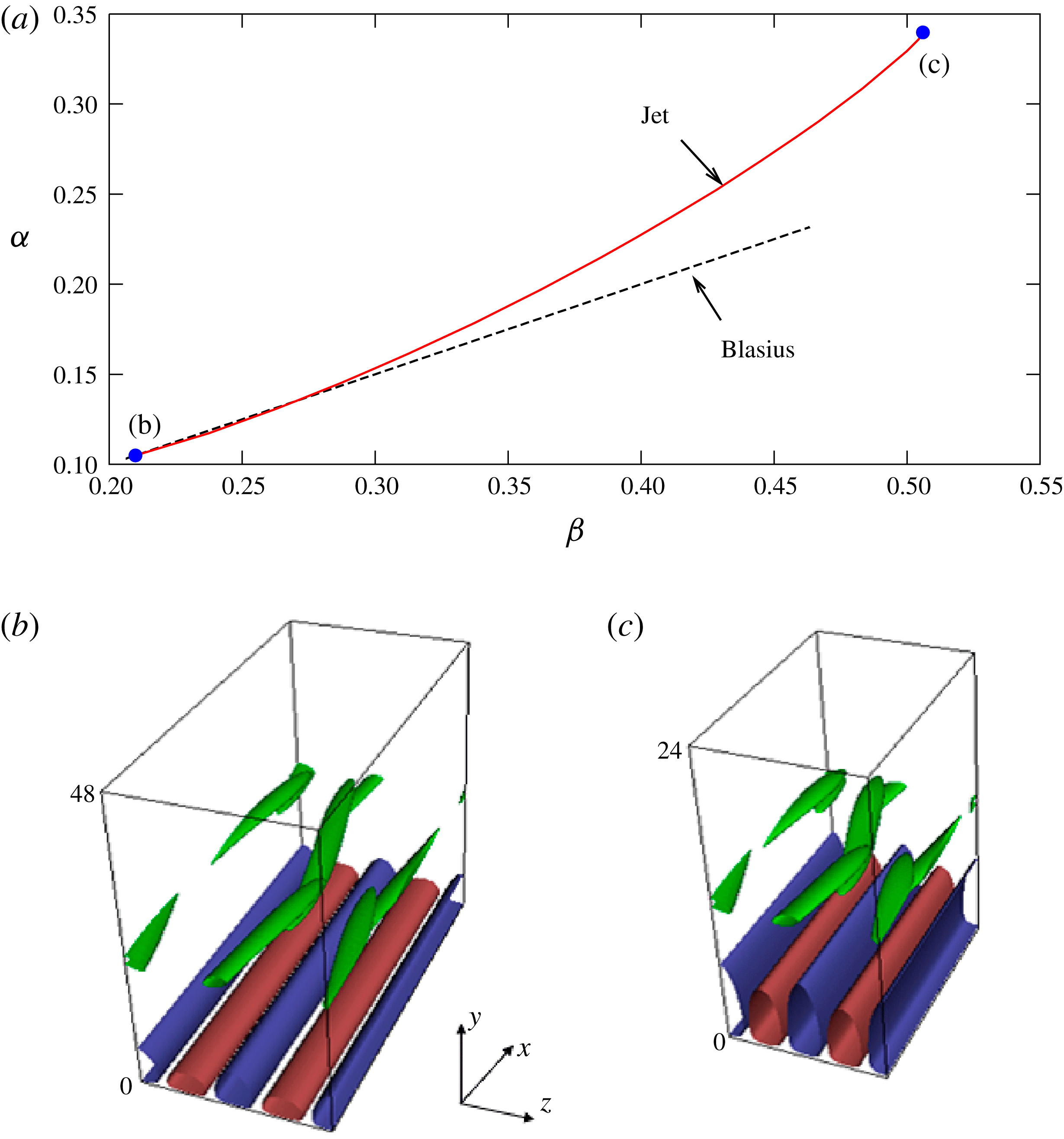
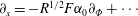
Figure 2. The travelling wave solutions of the ASBL problem. Note that the definition of the Reynolds number and the scale of the coordinates used here are different to those defined for the jet problem. (a) The wavenumbers selected in the computation. The red solid curve corresponds to the jet problem for
 $c\unicode[STIX]{x1D6FC}\unicode[STIX]{x1D6FD}^{-2}=120$
, whilst the dashed line corresponds to the results computed by Deguchi & Hall (Reference Deguchi and Hall2015a
) for Blasius problem
$c\unicode[STIX]{x1D6FC}\unicode[STIX]{x1D6FD}^{-2}=120$
, whilst the dashed line corresponds to the results computed by Deguchi & Hall (Reference Deguchi and Hall2015a
) for Blasius problem
 $\unicode[STIX]{x1D6FC}/\unicode[STIX]{x1D6FD}=0.5$
. Asymptotic convergence is checked in a range of Reynolds numbers from 100 000 to 200 000. The numbers of Fourier modes used in
$\unicode[STIX]{x1D6FC}/\unicode[STIX]{x1D6FD}=0.5$
. Asymptotic convergence is checked in a range of Reynolds numbers from 100 000 to 200 000. The numbers of Fourier modes used in
 $x$
and
$x$
and
 $z$
are 14 and 26, respectively. In the vertical direction 180 Chebyshev modes are used. (b,c) The flow field of the solutions at the corresponding points indicated in (a). The interval
$z$
are 14 and 26, respectively. In the vertical direction 180 Chebyshev modes are used. (b,c) The flow field of the solutions at the corresponding points indicated in (a). The interval
 $x\in [0,2\unicode[STIX]{x03C0}/\unicode[STIX]{x1D6FC}]$
,
$x\in [0,2\unicode[STIX]{x03C0}/\unicode[STIX]{x1D6FC}]$
,
 $z\in [0,2\unicode[STIX]{x03C0}/\unicode[STIX]{x1D6FD}]$
is used. The green surfaces are 50 % maximum absolute value of streamwise vorticity. The red/blue surfaces are 25 % maximum/minimum of streak, namely perturbation of streamwise velocity to the streamwise laminar flow,
$z\in [0,2\unicode[STIX]{x03C0}/\unicode[STIX]{x1D6FD}]$
is used. The green surfaces are 50 % maximum absolute value of streamwise vorticity. The red/blue surfaces are 25 % maximum/minimum of streak, namely perturbation of streamwise velocity to the streamwise laminar flow,
 $1-\text{e}^{-y}$
. Reynolds numbers used are (b)
$1-\text{e}^{-y}$
. Reynolds numbers used are (b)
 $100\,000$
, (c)
$100\,000$
, (c)
 $200\,000$
.
$200\,000$
.
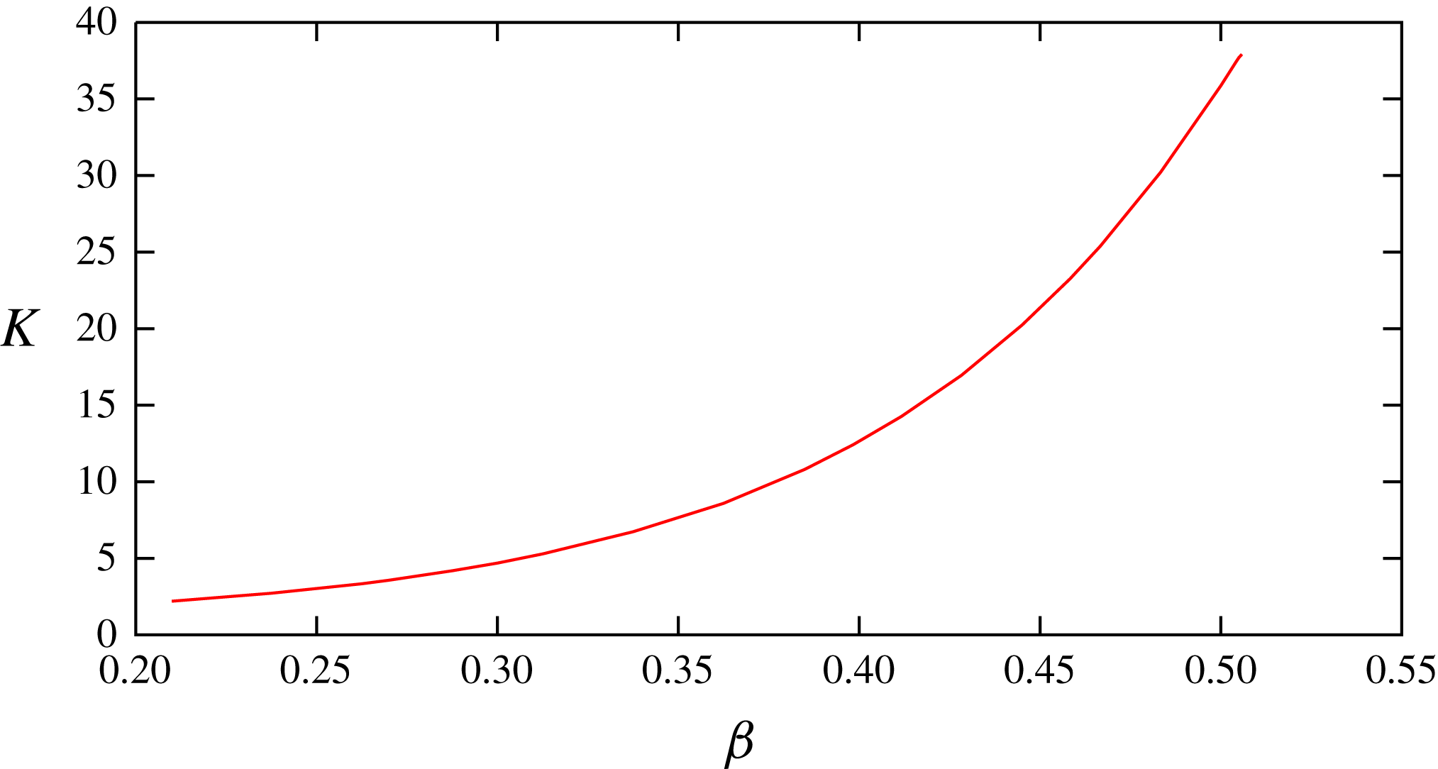
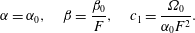
Figure 3. The value of
 $K$
along the solid red curve in figure 2(a).
$K$
along the solid red curve in figure 2(a).
Results of our computations for the case
 $c_{1}\unicode[STIX]{x1D6FC}\unicode[STIX]{x1D6FD}^{-2}=\unicode[STIX]{x1D6FA}_{0}\unicode[STIX]{x1D6FD}_{0}^{-2}=120$
are denoted by the red solid curve in figure 2(a). At any point on the curve the local value of
$c_{1}\unicode[STIX]{x1D6FC}\unicode[STIX]{x1D6FD}^{-2}=\unicode[STIX]{x1D6FA}_{0}\unicode[STIX]{x1D6FD}_{0}^{-2}=120$
are denoted by the red solid curve in figure 2(a). At any point on the curve the local value of
 $c_{1}$
is found from
$c_{1}$
is found from
 $c_{1}\unicode[STIX]{x1D6FC}\unicode[STIX]{x1D6FD}^{-2}=120$
. This solution curve was computed starting from the results for the Blasius problem given in Deguchi & Hall (Reference Deguchi and Hall2015a
), and shown by the black dashed line in the figure. Using Newton’s method we can continue the solution branch in a certain range of wavenumbers to find the corresponding locus of
$c_{1}\unicode[STIX]{x1D6FC}\unicode[STIX]{x1D6FD}^{-2}=120$
. This solution curve was computed starting from the results for the Blasius problem given in Deguchi & Hall (Reference Deguchi and Hall2015a
), and shown by the black dashed line in the figure. Using Newton’s method we can continue the solution branch in a certain range of wavenumbers to find the corresponding locus of
 $c_{1}\unicode[STIX]{x1D6FC}\unicode[STIX]{x1D6FD}^{-2}$
. The detail of the computational method is given in Deguchi & Hall (Reference Deguchi and Hall2014a
). The points (b) and (c) on the red solid curve are close to the saddle-node points where solutions appear; the flow visualisations at these points are given in figure 2(b,c). Throughout the paper the lower branch states are chosen to visualise the flow. The green surfaces represent the isosurfaces of the streamwise vorticity that shows the presence of free-stream coherent structures in the production layer. We have extracted that structure from the numerical result to construct the production layer solution of the jet problem. The blue and red surfaces show the induced near-wall streak by the free-stream coherent structures; these are the isosurfaces of the streamwise velocity deviation from the basic flow. Although these surfaces show the presence of the streak growth beneath the production layer, it should be noted that the near-wall part of the ASBL solution cannot be a good approximation of the jet problem because it takes no account of non-parallel effects.
$c_{1}\unicode[STIX]{x1D6FC}\unicode[STIX]{x1D6FD}^{-2}$
. The detail of the computational method is given in Deguchi & Hall (Reference Deguchi and Hall2014a
). The points (b) and (c) on the red solid curve are close to the saddle-node points where solutions appear; the flow visualisations at these points are given in figure 2(b,c). Throughout the paper the lower branch states are chosen to visualise the flow. The green surfaces represent the isosurfaces of the streamwise vorticity that shows the presence of free-stream coherent structures in the production layer. We have extracted that structure from the numerical result to construct the production layer solution of the jet problem. The blue and red surfaces show the induced near-wall streak by the free-stream coherent structures; these are the isosurfaces of the streamwise velocity deviation from the basic flow. Although these surfaces show the presence of the streak growth beneath the production layer, it should be noted that the near-wall part of the ASBL solution cannot be a good approximation of the jet problem because it takes no account of non-parallel effects.
3.3 Boundary layer analysis
Deguchi & Hall (Reference Deguchi and Hall2014a
) showed that as
 $Y\rightarrow -\infty$
the production layer solution behaves like
$Y\rightarrow -\infty$
the production layer solution behaves like
 $$\begin{eqnarray}\displaystyle & \displaystyle U\rightarrow -\text{e}^{-Y}-K(2\unicode[STIX]{x1D714})^{-1}\text{e}^{(\unicode[STIX]{x1D714}-1)Y}\cos (2\unicode[STIX]{x1D6FD}Z)+\cdots \,, & \displaystyle\end{eqnarray}$$
 $$\begin{eqnarray}\displaystyle & \displaystyle V\rightarrow -1+K\text{e}^{\unicode[STIX]{x1D714}Y}\cos (2\unicode[STIX]{x1D6FD}Z)+\cdots \,. & \displaystyle\end{eqnarray}$$
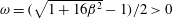 $\unicode[STIX]{x1D714}=(\sqrt{1+16\unicode[STIX]{x1D6FD}^{2}}-1)/2>0$
and therefore the exponential growth of the streak beneath the production layer is possible when
$\unicode[STIX]{x1D714}=(\sqrt{1+16\unicode[STIX]{x1D6FD}^{2}}-1)/2>0$
and therefore the exponential growth of the streak beneath the production layer is possible when
 $\unicode[STIX]{x1D6FD}<1/\sqrt{2}$
. We can confirm that the range of wavenumbers shown in figure 2(a) satisfies this condition. The coefficient
$\unicode[STIX]{x1D6FD}<1/\sqrt{2}$
. We can confirm that the range of wavenumbers shown in figure 2(a) satisfies this condition. The coefficient
 $K$
represents the intensity of the induced streak, and can be estimated by the numerical result as figure 3. We shall shortly see that this coefficient plays an important role in the computation of the asymptotic boundary layer problem. Reverting to the original variables, equation (3.8) becomes
$K$
represents the intensity of the induced streak, and can be estimated by the numerical result as figure 3. We shall shortly see that this coefficient plays an important role in the computation of the asymptotic boundary layer problem. Reverting to the original variables, equation (3.8) becomes  $$\begin{eqnarray}\displaystyle & \displaystyle u\rightarrow FG\text{e}^{-2\unicode[STIX]{x1D702}}+KF(GR^{1/2})^{-\unicode[STIX]{x1D714}}\frac{G}{2\unicode[STIX]{x1D714}}\text{e}^{(\unicode[STIX]{x1D714}-1)2\unicode[STIX]{x1D702}}\cos (2\unicode[STIX]{x1D6FD}_{0}z)+\cdots \,, & \displaystyle\end{eqnarray}$$
 $$\begin{eqnarray}\displaystyle & \displaystyle v\rightarrow -F+KF(GR^{1/2})^{-\unicode[STIX]{x1D714}}\text{e}^{\unicode[STIX]{x1D714}2\unicode[STIX]{x1D702}}\cos (2\unicode[STIX]{x1D6FD}_{0}z)+\cdots \,. & \displaystyle\end{eqnarray}$$
 $x$
derivatives are negligible to leading order, and thus the
$x$
derivatives are negligible to leading order, and thus the
 $x$
dependence remains parametric.
$x$
dependence remains parametric. In the boundary layer
 $u_{b}$
becomes
$u_{b}$
becomes
 $O(1)$
and thus the
$O(1)$
and thus the
 $x$
derivative in the convective term is no longer negligible. The leading-order equations are the Görtler vortex equations derived in Hall (Reference Hall1983, Reference Hall1988) with zero Görtler number:
$x$
derivative in the convective term is no longer negligible. The leading-order equations are the Görtler vortex equations derived in Hall (Reference Hall1983, Reference Hall1988) with zero Görtler number:
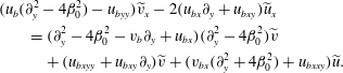
 $$\begin{eqnarray}\displaystyle & \displaystyle (\unicode[STIX]{x2202}_{t}+u\unicode[STIX]{x2202}_{x}+v\unicode[STIX]{x2202}_{y}+w\unicode[STIX]{x2202}_{z})u=u_{yy}+u_{zz}, & \displaystyle\end{eqnarray}$$
 $$\begin{eqnarray}\displaystyle & \displaystyle (\unicode[STIX]{x2202}_{t}+u\unicode[STIX]{x2202}_{x}+v\unicode[STIX]{x2202}_{y}+w\unicode[STIX]{x2202}_{z})v=-p_{y}+v_{yy}+v_{zz}, & \displaystyle\end{eqnarray}$$
 $$\begin{eqnarray}\displaystyle & \displaystyle (\unicode[STIX]{x2202}_{t}+u\unicode[STIX]{x2202}_{x}+v\unicode[STIX]{x2202}_{y}+w\unicode[STIX]{x2202}_{z})w=-p_{z}+w_{yy}+w_{zz}, & \displaystyle\end{eqnarray}$$
 $$\begin{eqnarray}\displaystyle & \displaystyle u_{x}+v_{y}+w_{z}=0. & \displaystyle\end{eqnarray}$$
 $x$
, and thus can be marched downstream given appropriate upstream conditions.
$x$
, and thus can be marched downstream given appropriate upstream conditions.If we expand
 $$\begin{eqnarray}\displaystyle & \displaystyle u=u_{b}+R^{-\unicode[STIX]{x1D714}/2}\widetilde{u}\cos (2\unicode[STIX]{x1D6FD}_{0}z)+\cdots \,, & \displaystyle\end{eqnarray}$$
 $$\begin{eqnarray}\displaystyle & \displaystyle v=v_{b}+R^{-\unicode[STIX]{x1D714}/2}\widetilde{v}\cos (2\unicode[STIX]{x1D6FD}_{0}z)+\cdots \,, & \displaystyle\end{eqnarray}$$
 $(\widetilde{u},\widetilde{v})$
are governed by the leading-order equations
$(\widetilde{u},\widetilde{v})$
are governed by the leading-order equations  $$\begin{eqnarray}\displaystyle u_{b}\widetilde{u}_{x}=(\unicode[STIX]{x2202}_{y}^{2}-4\unicode[STIX]{x1D6FD}_{0}^{2}-v_{b}\unicode[STIX]{x2202}_{y}-u_{bx})\widetilde{u}-u_{by}\widetilde{v}, & & \displaystyle\end{eqnarray}$$
 $$\begin{eqnarray}\displaystyle & & \displaystyle (u_{b}(\unicode[STIX]{x2202}_{y}^{2}-4\unicode[STIX]{x1D6FD}_{0}^{2})-u_{byy})\widetilde{v}_{x}-2(u_{bx}\unicode[STIX]{x2202}_{y}+u_{bxy})\widetilde{u}_{x}\nonumber\\ \displaystyle & & \displaystyle \qquad =(\unicode[STIX]{x2202}_{y}^{2}-4\unicode[STIX]{x1D6FD}_{0}^{2}-v_{b}\unicode[STIX]{x2202}_{y}+u_{bx})(\unicode[STIX]{x2202}_{y}^{2}-4\unicode[STIX]{x1D6FD}_{0}^{2})\widetilde{v}\nonumber\\ \displaystyle & & \displaystyle \qquad \quad +\,(u_{bxyy}+u_{bxy}\unicode[STIX]{x2202}_{y})\widetilde{v}+(v_{bx}(\unicode[STIX]{x2202}_{y}^{2}+4\unicode[STIX]{x1D6FD}_{0}^{2})+u_{bxxy})\widetilde{u}.\end{eqnarray}$$
 $(x,\unicode[STIX]{x1D702})$
and march in
$(x,\unicode[STIX]{x1D702})$
and march in
 $x$
applying the boundary conditions
$x$
applying the boundary conditions  $$\begin{eqnarray}\displaystyle & \displaystyle \widetilde{u}\rightarrow KFG^{1-\unicode[STIX]{x1D714}}(2\unicode[STIX]{x1D714})^{-1}\text{e}^{(\unicode[STIX]{x1D714}-1)2\unicode[STIX]{x1D702}},\quad \widetilde{v}\rightarrow KFG^{-\unicode[STIX]{x1D714}}\text{e}^{\unicode[STIX]{x1D714}2\unicode[STIX]{x1D702}},\quad \text{as}~\unicode[STIX]{x1D702}\rightarrow \infty , & \displaystyle\end{eqnarray}$$
 $$\begin{eqnarray}\displaystyle & \displaystyle \widetilde{u}_{y}=\widetilde{v}=0,\quad \text{at}~y=0, & \displaystyle\end{eqnarray}$$
 $y$
. The coefficient
$y$
. The coefficient
 $K(x)$
found from figure 3 and (3.6) describes the intensity of the forcing from the free-stream coherent structures. The numerical scheme to solve the marching problem is similar to that used in Deguchi & Hall (Reference Deguchi and Hall2015a
), where finite differences were used in vertical direction. In order to march the equations, the Adams–Bashforth method with step size
$K(x)$
found from figure 3 and (3.6) describes the intensity of the forcing from the free-stream coherent structures. The numerical scheme to solve the marching problem is similar to that used in Deguchi & Hall (Reference Deguchi and Hall2015a
), where finite differences were used in vertical direction. In order to march the equations, the Adams–Bashforth method with step size
 $10^{-6}$
is used, except for the diffusion terms, which are treated by the Crank–Nicolson method.
$10^{-6}$
is used, except for the diffusion terms, which are treated by the Crank–Nicolson method.
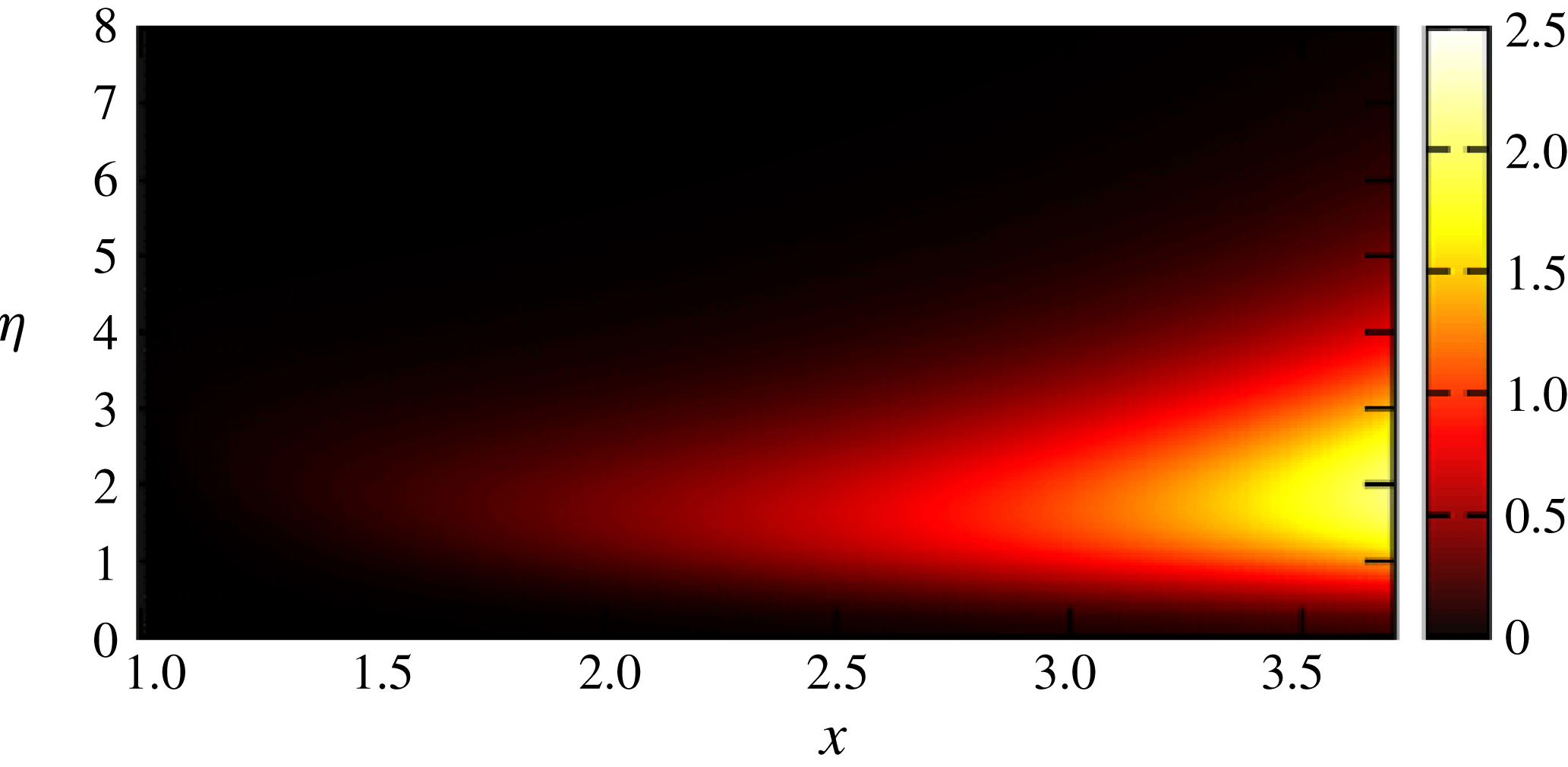
Figure 4. The streak amplitude
 $\widetilde{u}$
computed by the boundary layer asymptotic problem.
$\widetilde{u}$
computed by the boundary layer asymptotic problem.
We start the production layer interaction from the point (b) in figure 2(a). Without loss of generality we can choose the starting point at
 $x=1$
. We assume that before this point the flow is laminar. That choice of the starting point requires us to select the parameters of the global problem as
$x=1$
. We assume that before this point the flow is laminar. That choice of the starting point requires us to select the parameters of the global problem as
 $\unicode[STIX]{x1D6FD}_{0}=0.21\times 2/3=0.14$
; see (3.6). Also, since we fix
$\unicode[STIX]{x1D6FD}_{0}=0.21\times 2/3=0.14$
; see (3.6). Also, since we fix
 $\unicode[STIX]{x1D6FA}_{0}\unicode[STIX]{x1D6FD}_{0}^{-2}=120$
to solve the production layer problem,
$\unicode[STIX]{x1D6FA}_{0}\unicode[STIX]{x1D6FD}_{0}^{-2}=120$
to solve the production layer problem,
 $\unicode[STIX]{x1D6FA}_{0}=120\times 0.14^{2}=2.352$
. The resultant streak amplitude solution
$\unicode[STIX]{x1D6FA}_{0}=120\times 0.14^{2}=2.352$
. The resultant streak amplitude solution
 $\widetilde{u}$
is shown in figure 4. Here we used 400 points in
$\widetilde{u}$
is shown in figure 4. Here we used 400 points in
 $\unicode[STIX]{x1D702}\in [0,8]$
, but the result is insensitive to the number of points and the upper bound of the vertical domain size. Consistent with the theory we see that a large-amplitude streak is generated. The origin of the streak growth is the last term in (3.12a
), where the small vertical perturbation velocity interacts with the basic flow. The vertical perturbation decays exponentially towards the centre of the jet, but since the basic flow grows at faster rate, the forcing term becomes large in the boundary layer. However, the basic flow growth is suppressed when
$\unicode[STIX]{x1D702}\in [0,8]$
, but the result is insensitive to the number of points and the upper bound of the vertical domain size. Consistent with the theory we see that a large-amplitude streak is generated. The origin of the streak growth is the last term in (3.12a
), where the small vertical perturbation velocity interacts with the basic flow. The vertical perturbation decays exponentially towards the centre of the jet, but since the basic flow grows at faster rate, the forcing term becomes large in the boundary layer. However, the basic flow growth is suppressed when
 $\unicode[STIX]{x1D702}$
becomes small, and thus the growth of the streak is also suppressed there as well.
$\unicode[STIX]{x1D702}$
becomes small, and thus the growth of the streak is also suppressed there as well.
4 Conclusion and discussions
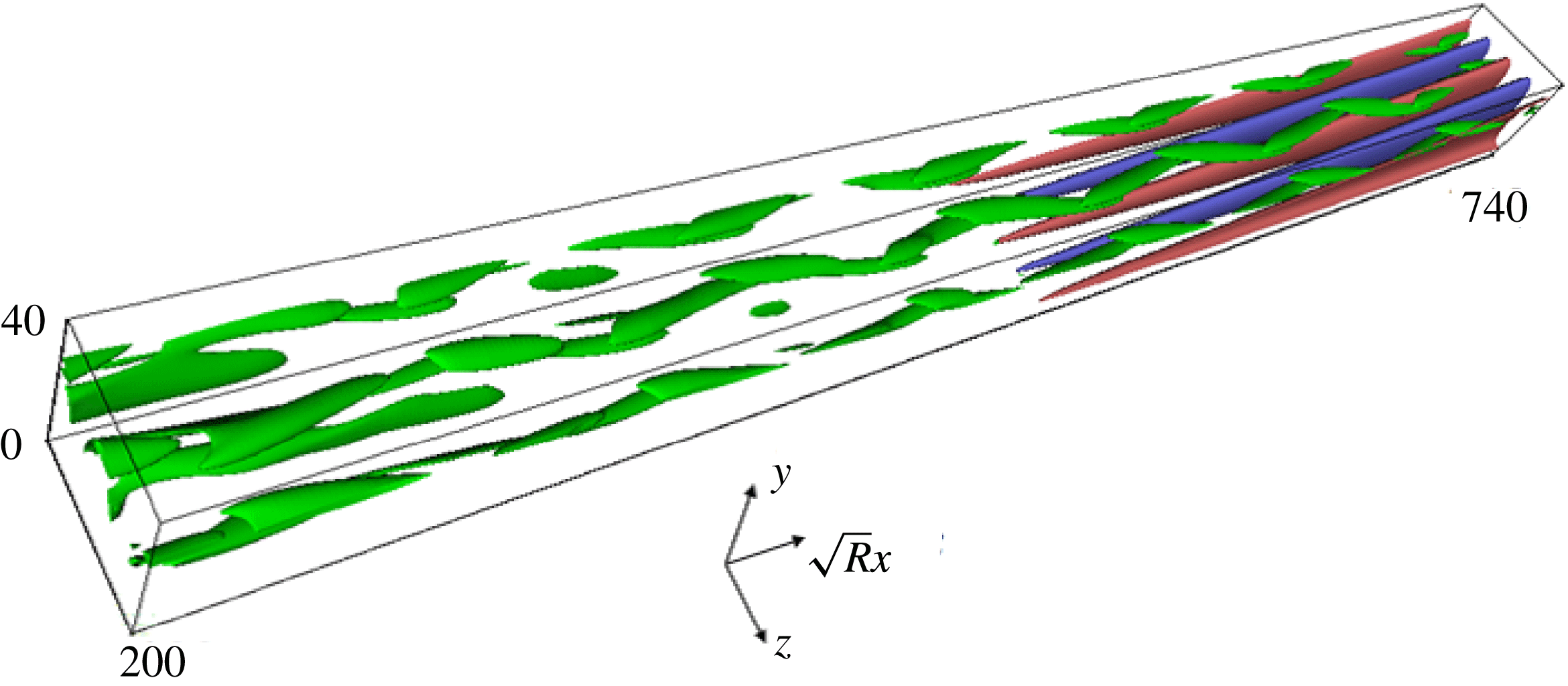
Figure 5. Combined plot of the free-stream coherent structures for the planar jet;
 $(R,\unicode[STIX]{x1D6FD}_{0},\unicode[STIX]{x1D6FA}_{0})=(40\,000,0.14,2.352)$
. The interval
$(R,\unicode[STIX]{x1D6FD}_{0},\unicode[STIX]{x1D6FA}_{0})=(40\,000,0.14,2.352)$
. The interval
 $x\in [1,3.7]$
,
$x\in [1,3.7]$
,
 $z\in [0,2\unicode[STIX]{x03C0}/\unicode[STIX]{x1D6FD}_{0}]$
is used. The green surface represents the 25 % maximum of the absolute streamwise vorticity computed by the ASBL solutions. The red/blue surfaces are positive/negative isocontours of the streak, where the 25 % maximum/minimum of the streamwise perturbation velocity is visualised.
$z\in [0,2\unicode[STIX]{x03C0}/\unicode[STIX]{x1D6FD}_{0}]$
is used. The green surface represents the 25 % maximum of the absolute streamwise vorticity computed by the ASBL solutions. The red/blue surfaces are positive/negative isocontours of the streak, where the 25 % maximum/minimum of the streamwise perturbation velocity is visualised.
In this paper we have for the first time presented a high-Reynolds-number asymptotic representation of three-dimensional nonlinear periodic solutions in a free planar jet. A matched asymptotic expansion of Navier–Stokes equations was used to derive the Reynolds-number-independent problem in the production layer and the boundary layer; see figure 1. In the production layer the flow is governed by the canonical problem derived previously for ASBL and many other boundary layer flows. At each streamwise position, the solution of the asymptotic problem can be found from direct Navier–Stokes solutions of ASBL using the implicit relationship between local spanwise and streamwise wavenumbers. The coherent vortices localised in the production layer produce a streaky field growing towards the centre of the jet. In the boundary layer near the centre of the jet the non-parallel effect plays dominant role, and thus we must integrate the asymptotic equations in the streamwise direction subject to the forcing from the production layer.
The configuration concerned in this paper is the simplest jet flow, and in fact is the simplest free-stream coherent structure theory in the presence of non-parallel effects. The solution in the boundary layer depends on the upstream condition, as pointed out for the Görtler problem by Hall (Reference Hall1983). On the other hand, in the production layer the free-stream coherent structures fix the form and size of the upstream condition to maintain the periodic solutions in the jet; if the upstream input in the free stream is perturbed, the downstream flow may become turbulent or laminar. In an experiment, the upstream perturbation in the free stream could be related to the perturbation from the jet nozzle.
Given the asymptotic solutions obtained in the previous section, we can construct the combined picture of the overall periodic solution for arbitrary Reynolds numbers. Figure 5 is a snapshot of the combined solution for
 $R=40\,000$
. The green surfaces visualise the free-stream coherent structures constructed from (3.4) to (3.6), where
$R=40\,000$
. The green surfaces visualise the free-stream coherent structures constructed from (3.4) to (3.6), where
 $\boldsymbol{U}(\unicode[STIX]{x1D6F7},Y,Z)$
can be obtained by rescaling large-Reynolds-number ASBL solutions in figure 2; see Deguchi & Hall (Reference Deguchi and Hall2014a
). The global solution inherits the appearance of the lambda-shaped coherent vortices seen in the ASBL solutions, and is reminiscent of that seen in figures 3 and 4 of Sakakibara & Anzai (Reference Sakakibara and Anzai2001). The red/blue surfaces sitting below the coherent vortices are the fast/slow streaks obtained from (3.11a
) using the function
$\boldsymbol{U}(\unicode[STIX]{x1D6F7},Y,Z)$
can be obtained by rescaling large-Reynolds-number ASBL solutions in figure 2; see Deguchi & Hall (Reference Deguchi and Hall2014a
). The global solution inherits the appearance of the lambda-shaped coherent vortices seen in the ASBL solutions, and is reminiscent of that seen in figures 3 and 4 of Sakakibara & Anzai (Reference Sakakibara and Anzai2001). The red/blue surfaces sitting below the coherent vortices are the fast/slow streaks obtained from (3.11a
) using the function
 $\widetilde{u}(x,y)$
computed in figure 3. As explained in the asymptotic theory, the driving mechanism of the streak is the forcing from the vortices modulated by the non-parallel effect. The formation of the streaky field by pairs of counter-rotating streamwise vortices is the typical flow topology of the three-dimensional coherent structures observed in turbulent jet experiments and simulations; see Liepmann & Morteza (Reference Liepmann and Morteza1992), Fureby & Grinstein (Reference Fureby and Grinstein2002), Kozlov et al. (Reference Kozlov, Grek, Löfdahl, Chernorai and Litvinenko2002), Jung et al. (Reference Jung, Gamard and George2004), Ball et al. (Reference Ball, Fellouah and Pollard2012), for example. It has been pointed in the experimental literature that the turbulent–laminar interface is highly convoluted. The production layer is in fact the position where the most complicated flow structure could be observed, as all the terms in the Navier–Stokes equations must be retained there even at the large-Reynolds-number limit. The production layer structure used in this paper is rather simple, but note that the problem could possess more complicated nonlinear solutions other than the one we have shown in this paper. Therefore, in view of the remarks made above, we conclude that the overall structure of our solution is qualitatively consistent with previous observations in experiments and simulations.
$\widetilde{u}(x,y)$
computed in figure 3. As explained in the asymptotic theory, the driving mechanism of the streak is the forcing from the vortices modulated by the non-parallel effect. The formation of the streaky field by pairs of counter-rotating streamwise vortices is the typical flow topology of the three-dimensional coherent structures observed in turbulent jet experiments and simulations; see Liepmann & Morteza (Reference Liepmann and Morteza1992), Fureby & Grinstein (Reference Fureby and Grinstein2002), Kozlov et al. (Reference Kozlov, Grek, Löfdahl, Chernorai and Litvinenko2002), Jung et al. (Reference Jung, Gamard and George2004), Ball et al. (Reference Ball, Fellouah and Pollard2012), for example. It has been pointed in the experimental literature that the turbulent–laminar interface is highly convoluted. The production layer is in fact the position where the most complicated flow structure could be observed, as all the terms in the Navier–Stokes equations must be retained there even at the large-Reynolds-number limit. The production layer structure used in this paper is rather simple, but note that the problem could possess more complicated nonlinear solutions other than the one we have shown in this paper. Therefore, in view of the remarks made above, we conclude that the overall structure of our solution is qualitatively consistent with previous observations in experiments and simulations.
Nevertheless, it should be noticed that direct quantitative comparison of our solutions with the existent turbulent experimental results such as Deo et al. (Reference Deo, Mi and Nathan2008) is not easily done. The difficulty is twofold. The first difficulty is that the periodic solution we have, for example, constructed in figure 5 is the simplest nonlinear flow where the background flow remains not too far from the analytic laminar flow profile. The key point in the dynamical systems theory point of view of turbulence is that turbulence can be understood by a weighted sum of periodic solutions, because turbulent trajectories in the phase space recurrently visit various periodic solutions; see Cvitanović (Reference Cvitanović2013), for example. For relatively low Reynolds numbers, Kawahara & Kida (Reference Kawahara and Kida2001) showed that only one periodic solution gives an excellent approximation of the turbulent statistics of the flow. However, for large Reynolds numbers the dynamical systems theory picture of turbulence is much more complicated, as there are a myriad of solutions with possibly distinct asymptotic structures. Therefore, our solutions must be regarded as one of the building blocks to describe large-Reynolds-number dynamics of jet flows, in the sense that they can only capture some aspects of the dynamics.
The second difficulty is the inviscid instability of the laminar basic flow due to the inflection point of the flow. In fact inviscid instability mechanisms seem to be very powerful in the jet flows; for example, in the round jet experiments the origin of the observed helical modes were explained by the local linear stability of the mean flow (Liepmann & Morteza Reference Liepmann and Morteza1992; Jung et al. Reference Jung, Gamard and George2004; Iqbal & Thomas Reference Iqbal and Thomas2007). Once the mode is generated in the flow, the instability might well dominate other smaller-scale vortices including free-stream coherent structures. Since the streaky field generated by the free-stream coherent structures may be subdominant in turbulence, some special control technique must be employed in the experiment. For inviscidly stable class of flows in channel or pipe, a simple successful flow control technology has been developed to directly observe periodic solutions in experiments/simulations; see Itano & Toh (Reference Itano and Toh2001), de Lozar et al. (Reference de Lozar, Mellibovsky, Avila and Hof2012). However, the linear instability of the basic jet flow even at low Reynolds numbers may present a difficulty in observing our solutions in their pure form.
The prediction by the asymptotic model may be extended by including the above effects missing in the present theory. For example, we can consider the interaction of the inviscid instability with the free-stream coherent structures. That interaction might produce significant problems able to describe more quantitative results for large-Reynolds-number fully developed turbulent jet flows. The feedback effect from the inviscid wave from the background flow may be considered in a similar manner as the vortex–wave interaction theory by Hall & Smith (Reference Hall and Smith1991). The distortion of the background flow possibly changes the position of the production layer, and then the effect of the free-stream coherent structures on the jet centre through the growing streak would be altered. Moreover, although application of the present theory to the axisymmetric jet may be of interest from a practical point of view, it also needs some extension of the theory. For example, in view of the experimental observations, the use of helical coordinate seems crucial in order for a better flow prediction. The asymptotic description of oblique vortical structures in shear flows given by Deguchi & Hall (Reference Deguchi and Hall2015b ) could be used to describe such helical flows. Another ingredient missing in our theory is the effect of the jet nozzle. As remarked in § 1, it is well-known from the experimental observation that axisymmetric vortices produced by Kelvin–Helmholtz instability at the lip of round jet nozzle are the dominant flow structures in the initial development of jet flows. In the planar jet, the analogous result corresponds to the initial development of the quasi-spanwise vortices placed anti-symmetrically near the jet centre. The three-dimensional breakdown of such vortices is an alternative significant source of streaky flow. Thus, the excitation of the breakdown by the free-stream coherent structures is of obvious interest; such an excitation of instability by external effects is called receptivity. It would be noteworthy that recently Deguchi & Hall (Reference Deguchi and Hall2017) and Dempsey, Hall & Deguchi (Reference Dempsey, Hall and Deguchi2017) found that the free-stream coherent structures are remarkably efficient generator of streaks in boundary layer flows over a curved wall, through the receptivity mechanism. Although any above extension is of interest, it makes the theory extremely complicated, and thus mathematical consistency would be increasingly difficult to maintain. The computation of the production layer structure is already challenging, and thus further extension of the asymptotic model would make the numerical work formidable. As our aim in this paper is to describe the basic idea of the new theory in its simplest form, we leave those further analyses to future work.
Finally, we comment on the possible relevance of this work to jet acoustics. High-frequency noise from a compressible jet is attributed to short-scale turbulent structures within the jet. Low-frequency noise is associated with hydrodynamic instabilities of the mean part of the turbulent jet flow. The implication of our analysis here to round compressible jets is that low-frequency noise could be generated a long way from the centre of the jet, and that it would depend crucially on how the jet adjusted to its free-stream value. The frequency of the waves generated would be small because the nonlinear waves in the production layer move downstream slowly. Therefore, the mechanism we describe here can provide an alternative source of low-frequency noise from a compressible jet.
Acknowledgements
The first author is the recipient of an Australian Research Council Australian Discovery Early Career Award DE170100171 funded by the Australian Government. This research was partially supported by EPSRC through the grant EP/I037946/1. The constructive comments made by the referees are gratefully acknowledged.


