2. Problem formulation

Let us consider a perfect gas flow past a flat plate that is aligned with the mean velocity vector in the free stream; see figure 1. We shall assume that small-amplitude entropy waves are present in the oncoming flow. We shall further assume that there is a small roughness on the plate surface at distance $L$ from the leading edge. In what follows we shall assume that the flow is two-dimensional. To study the flow we use the Cartesian coordinates $(\hat {x}, \hat {y})$, with $\hat {x}$ measured along the flat plate surface from its leading edge $O$, and $\hat {y}$ in the perpendicular direction. The velocity components in these coordinates are denoted by $(\hat {u} , \hat {v})$. As usual, we denote the time by $\hat {t}$, the gas density by $\hat {\rho }$, pressure by $\hat {p}$, enthalpy by $\hat {h}$ and dynamic viscosity coefficient by $\hat {\mu }$. The ‘hat’ is used here for dimensional variables. The non-dimensional variables are introduced as follows:

(2.1) \begin{equation} \left. \begin{aligned} \hat{t} &= \dfrac{L}{V_{\infty }} t , & \hat{x} &= L x , & \hat{y}&= L y ,\\ \hat{u} &= V_{\infty } u , & \hat{v} &= V_{\infty } v, & \hat{\rho } &= \rho _{\infty } \rho ,\\ \hat{p} &= p_{\infty } + \rho _{\infty } V_{\infty }^2 p , & \hat{h} &= V_{\infty }^2 h, & \hat{\mu } &= \mu _{\infty } \mu,\end{aligned} \right\} \end{equation}

with $V_{\infty }$, $p_{\infty }$, $\rho _{\infty }$ and $\mu _{\infty }$ being the dimensional free-stream velocity, pressure, density and viscosity, respectively.

Figure 1. Flow layout.

In the non-dimensional variables, the Navier–Stokes equations are written as

(2.2a)$$\begin{gather} \rho \left( \frac{\partial u}{\partial t} + u \frac{\partial u}{\partial x} + v \frac{\partial u}{\partial y} \right) ={-} \frac{\partial p}{\partial x} + \frac{1}{Re} \left\{ \frac{\partial }{\partial x} \left[ \mu \left( \frac{4}{3} \frac{\partial u} {\partial x} - \frac{2}{3} \frac{\partial v}{\partial y} \right) \right] \right. \nonumber\\ \left. + \frac{\partial }{\partial y} \left[ \mu \left( \frac{\partial u}{\partial y} + \frac{\partial v}{\partial x} \right) \right] \right\},\end{gather}$$

(2.2b)$$\begin{gather} \rho \left( \frac{\partial v}{\partial t} + u \frac{\partial v}{\partial x} + v \frac{\partial v}{\partial y} \right) ={-} \frac{\partial p}{\partial y} + \frac{1}{Re} \left\{ \frac{\partial }{\partial y} \left[ \mu \left( \frac{4}{3} \frac{\partial v} {\partial y} - \frac{2}{3} \frac{\partial u}{\partial x} \right) \right]\right. \nonumber\\ \left. + \frac{\partial }{\partial x} \left[ \mu \left( \frac{\partial u}{\partial y} + \frac{\partial v}{\partial x} \right) \right] \right\},\end{gather}$$

(2.2c)$$\begin{gather} \rho \left( \frac{\partial h}{\partial t} + u \frac{\partial h}{\partial x} + v \frac{\partial h}{\partial y} \right) = \frac{\partial p}{\partial t} + u \frac{\partial p}{\partial x} + v \frac{\partial p}{\partial y} + \frac{1}{Re} \left\{ \frac{1}{Pr} \left[ \frac{\partial }{\partial x} \left( \mu \frac{\partial h}{\partial x} \right) + \frac{\partial }{\partial y} \left( \mu \frac{\partial h}{\partial y} \right) \right]\right. \nonumber\\ \left. + \mu \left( \frac{4}{3} \frac{\partial u}{\partial x} - \frac{2}{3} \frac{\partial v}{\partial y} \right) \frac{\partial u}{\partial x} + \mu \left( \frac{4}{3} \frac{\partial v}{\partial y} - \frac{2}{3} \frac{\partial u}{\partial x} \right) \frac{\partial v}{\partial y} + \mu \left( \frac{\partial u}{\partial y} + \frac{\partial v}{\partial x} \right) ^2 \right\} ,\end{gather}$$

(2.2d)$$\begin{gather}\frac{\partial \rho }{\partial t} + \frac{\partial \rho u}{\partial x} + \frac{\partial \rho v}{\partial y} = 0 , \end{gather}$$

(2.2e)$$\begin{gather}h = \frac{1}{(\gamma - 1) M_{\infty }^2} \frac{1}{\rho } + \frac{\gamma } {\gamma -1} \frac{p}{\rho } . \end{gather}$$

Here, $Pr$ is the Prandtl number and $\gamma$ is the specific heat ratio; for air $Pr \approx 0.713$, $\gamma = 7/5$. The Reynolds number $Re$ is calculated as

(2.3)\begin{equation} Re = \frac{\rho _{\infty } V_{\infty } L}{\mu _{\infty }} . \end{equation}

In this study, we shall assume that $Re$ is large, while the free-stream Mach number, $M_{\infty } = V_{\infty } / a_{\infty }$, remains finite. In fact, we shall restrict our attention to the subsonic flows where $M_{\infty } < 1$.

3. Unperturbed flow

Our first task is to describe the steady unperturbed flow. At large values of the Reynolds number, the boundary-layer theory of Prandtl (Reference Prandtl1904) can be used for this purpose. According to this theory, the flow field should be divided into two regions: the inviscid region occupying the majority of the flow and the thin boundary layer that forms on the surface of the plate. In the inviscid region, the flow remains unperturbed in the leading-order approximation with the fluid-dynamic functions preserving their values in the oncoming flow before the plate

(3.1a–e)\begin{equation} u = 1 , \quad v = 0 , \quad p = 0 , \quad \rho = 1 , \quad h = \frac{1}{(\gamma - 1) M_{\infty }^2} . \end{equation}

When dealing with the boundary layer we assume that

(3.2a–c)\begin{equation} x = O(1) , \quad Y = Re^{1/2} y = O(1) , \quad Re \to \infty , \end{equation}

and represent the corresponding solution of the Navier–Stokes equations (2.2) in the form

(3.3)\begin{equation} \left. \begin{aligned} u (t , x , y ; Re) & = U_0 (x , Y) + \cdots , \quad v (t , x , y ; Re) = Re^{{-}1/2} V_0 (x , Y) + \cdots , \\ \rho (t , x , y ; Re) & = \rho_0 (x , Y) + \cdots , \quad p (t , x , y ; Re) = Re^{{-}1/2} P_0 (x , Y) + \cdots , \\ h (t , x , y ; Re) & = h_0 (x , Y) + \cdots , \quad \mu (t , x , y ; Re) = \mu _0 (x , Y) + \cdots . \end{aligned} \right\} \end{equation}

Substitution of (3.3) into the Navier–Stokes equations (2.2) leads to classical boundary-layer equations for compressible flow. A detailed discussion of these equations together with corresponding boundary conditions may be found in § 1.10 in the book by Ruban (Reference Ruban2018). We shall assume here that the plate surface is thermally isolated, in which case the boundary-layer equations admit a self-similar solution in the form

(3.4)\begin{equation} \left. \begin{gathered} U_0 (x , Y) = \tilde{U} (\eta ) , \quad V_0 (x , Y) = \frac{1}{\sqrt{x}} \tilde{V} (\eta ) , \quad \rho _0 (x , Y) = \tilde{\rho } (\eta ) , \\ h_0 (x , Y) = \tilde{h} (\eta ) , \quad \mu _0 (x , Y) = \tilde{\mu } (\eta ) , \end{gathered} \right\} \end{equation}

where

(3.5)\begin{equation} \eta = \frac{Y}{\sqrt{x}} . \end{equation}

Functions $\tilde {U}$, $\tilde {V}$, $\tilde {h}$ and $\tilde {\rho }$ are to be found by solving the following set of ordinary differential equations:

(3.6a)$$\begin{gather} - \frac{1}{2} \eta \tilde{\rho } \tilde{U} \frac{\textrm{d} \tilde{U}}{\textrm{d} \eta } + \tilde{\rho } \tilde{V} \frac{\textrm{d} \tilde{U}}{\textrm{d} \eta } = \frac{\textrm{d}}{\textrm{d} \eta } \left( \tilde{\mu } \frac{\textrm{d} \tilde{U}}{\textrm{d} \eta } \right) , \end{gather}$$

(3.6b)$$\begin{gather}- \frac{1}{2} \eta \tilde{\rho } \tilde{U} \frac{\textrm{d} \tilde{h}}{\textrm{d} \eta } + \tilde{\rho } \tilde{V} \frac{\textrm{d} \tilde{h}}{\textrm{d} \eta } = \frac{1}{Pr} \frac{\textrm{d}} {\textrm{d} \eta } \left( \tilde{\mu } \frac{\textrm{d} \tilde{h}}{\textrm{d} \eta } \right) + \tilde{\mu } \left( \frac{\textrm{d} \tilde{U}}{\textrm{d} \eta } \right) ^2 , \end{gather}$$

(3.6c)$$\begin{gather}- \frac{1}{2} \eta \frac{d}{d \eta } (\tilde{\rho } \tilde{U}) + \frac{\textrm{d}}{\textrm{d}\eta} (\tilde{\rho } \tilde{V}) = 0 , \end{gather}$$

(3.6d)$$\begin{gather}\tilde{h} = \frac{1}{(\gamma - 1) M_{\infty }^2} \frac{1}{\tilde{\rho }}, \end{gather}$$

subject to the boundary conditions

(3.6e)$$\begin{gather} \tilde{U} = 1 , \quad \tilde{h} = \frac{1}{(\gamma - 1) M_{\infty }^2} \quad \text{at} \ \eta = \infty , \end{gather}$$

(3.6f)$$\begin{gather}\tilde{U} = \tilde{V} = 0 , \quad \frac{\textrm{d} \tilde{h}}{\textrm{d} \eta } = 0, \quad \text{at} \ \eta = 0 . \end{gather}$$

To perform the receptivity analysis of the boundary layer, we need to know the behaviour of the solution to (3.6) near the plate surface ($\eta \to 0$) and at the outer edge of the boundary layer ($\eta \to \infty$). In view of (3.6f) the Taylor expansions of $\tilde {U}$ and $\tilde {h}$ near the plate surface may be written as

(3.7)\begin{equation} \tilde{U} = \lambda \eta + \cdots , \quad \tilde{h} = h_w + O (\eta ^2), \quad \text{as} \ \eta \to 0 , \end{equation}

where constants $\lambda$ and $h_w$ are found through a numerical solution of the boundary value problem (3.6).

To describe the behaviour of the solution near the outer edge of the boundary layer we use the procedure suggested in problem 2 in exercises 1 in Ruban (Reference Ruban2018). We find that

(3.8)\begin{equation} \tilde{U} = 1 - \frac{C}{2 (\eta - B)} \, \textrm{e}^{-(\eta - B)^2 / 4} + \cdots , \quad \text{as} \ \eta \to \infty . \end{equation}

Constants $C$ and $B$ are found through numerical solution of (3.6) as a whole.

4. Entropy waves

The flow upstream of the leading edge of the plate and in the inviscid region above the plate is given in the leading-order approximation by (3.1a–e). We shall now perturb this flow

(4.1)\begin{equation} \left. \begin{gathered} u = 1 + \varepsilon u^{\prime } (t , x , y) , \quad v = \varepsilon v^{\prime } (t , x , y) , \quad \rho = 1 + \varepsilon \rho ^{\prime } (t , x , y) , \\ p = \varepsilon p^{\prime } (t , x , y) , \quad h = \frac{1}{(\gamma - 1) M_{\infty }^2} + \varepsilon h^{\prime } (t , x , y) , \end{gathered} \right\} \end{equation}

where $\varepsilon$ is a small parameter representing the amplitude of the perturbations.

Substituting (4.1) into the Navier–Stokes equations (2.2) and working with the $O (\varepsilon )$ terms we arrive at the linearised Euler equations

(4.2)\begin{equation} \left. \begin{gathered} \frac{\partial u^{\prime }}{\partial t} + \frac{\partial u^{\prime }}{\partial x} ={-} \frac{\partial p^{\prime }}{\partial x} , \\ \frac{\partial v^{\prime }}{\partial t} + \frac{\partial v^{\prime }}{\partial x} ={-} \frac{\partial p^{\prime }}{\partial y} , \\ \frac{\partial h^{\prime }}{\partial t} + \frac{\partial h^{\prime }}{\partial x} = \frac{\partial p^{\prime }}{\partial t} + \frac{\partial p^{\prime }}{\partial x} , \\ \frac{\partial \rho ^{\prime }}{\partial t} + \frac{\partial \rho ^{\prime }} {\partial x} + \frac{\partial u^{\prime }}{\partial x} + \frac{\partial v^{\prime }} {\partial y} = 0 ,\\ h^{\prime } = \frac{\gamma }{\gamma - 1} p^{\prime } - \frac{1}{(\gamma - 1) M_{\infty }^2} \rho ^{\prime } . \end{gathered} \right\} \end{equation}

According to Kovasznay (Reference Kovasznay1953), an arbitrary small perturbation to uniform compressible flow can be represented as a superposition of acoustic noise, vorticity waves and entropy waves. If the amplitude of these modes is small, then they may be considered independent of one another. As was already mentioned, the generation of the Tollmien–Schlichting waves by acoustic noise and by vorticity waves were studied by Ruban (Reference Ruban1984) and Goldstein (Reference Goldstein1985) and by Duck et al. (Reference Duck, Ruban and Zhikharev1996), respectively. In this paper, we are concerned with the entropy waves, where

(4.3)\begin{equation} u^{\prime } = v^{\prime } = p^{\prime } = 0 , \end{equation}

and (4.2) reduce to

(4.4a)$$\begin{gather} \frac{\partial h^{\prime }}{\partial t} + \frac{\partial h^{\prime }}{\partial x} = 0 , \end{gather}$$

(4.4b)$$\begin{gather}\frac{\partial \rho ^{\prime }}{\partial t} + \frac{\partial \rho ^{\prime }} {\partial x} = 0 , \end{gather}$$

(4.4c)$$\begin{gather}h^{\prime } ={-} \frac{1}{(\gamma - 1) M_{\infty }^2} \rho ^{\prime } . \end{gather}$$

The general solutions to (4.4a), (4.4b) are written as

(4.5a,b)\begin{equation} h^{\prime } = f (x - t , y) , \quad \rho ^{\prime } = g (x - t , y) , \end{equation}

which shows that the entropy waves propagate downstream with the mean free-stream velocity. We shall assume that the free-stream turbulence is uniform, in which case $h^{\prime }$ and $\rho ^{\prime }$ can be represented as a superposition of the Fourier harmonics

(4.6a,b) \begin{align} h^{\prime } &= \sum_{i,j} h_{i,j} \exp\left({\textrm{i} [\alpha _i (x - t) + \beta _j y]}\right) + (\textrm{c.c.}) ,\nonumber\\ \rho^{\prime } &= \sum_{i,j} \rho _{i,j} \exp\left({\textrm{i} [\alpha _i (x - t) + \beta _j y]}\right) + (\textrm{c.c.}), \end{align}

where the longitudinal and lateral wavenumbers, $\alpha _i$ and $\beta _j$, are real, and $(\textrm {c.c.})$ denotes the complex conjugate of the quantity in front of it. For efficient receptivity, only the harmonics that are in resonance with the Tollmien–Schlichting waves are important, namely, have an $O (Re^{1/4})$ frequency. Keeping this in mind, we introduce the ‘fast’ time and coordinates

(4.7a–c)\begin{equation} \bar{t} = Re^{1/4} t , \quad \bar{x} = Re^{1/4} x , \quad \bar{y} = Re^{1/4} y , \end{equation}

and consider a harmonic from (4.6a,b). We can express it in the form

(4.8a,b)\begin{equation} h^{\prime } = h_a \exp\left({\textrm{i} \alpha \xi + \beta \bar{y}}\right) + (\textrm{c.c.}) , \quad \rho ^{\prime } = \rho _a \exp\left({\textrm{i} \alpha \xi + \beta \bar{y}}\right) + (\textrm{c.c.}) , \end{equation}

where

(4.9)\begin{equation} \xi = \bar{x} - \bar{t} . \end{equation}

It follows from (4.4c) that $h_a$ and $\rho _a$ are related to one another as

(4.10)\begin{equation} \rho _a={-} (\gamma - 1) M_{\infty }^2 h_a . \end{equation}

Through appropriate adjustment of the amplitude parameter $\varepsilon$ in (4.1) we can always make $\rho _a = 1$, and then we will have

(4.11a,b)\begin{equation} h^{\prime } ={-} \frac{1}{(\gamma - 1) M_{\infty }^2} \exp\left({\textrm{i} \alpha \xi + \beta \bar{y}}\right) + (\textrm{c.c.}) , \quad \rho ^{\prime } = \exp\left({\textrm{i} \alpha \xi + \beta \bar{y}}\right) + (\textrm{c.c.}) . \end{equation}

5. Transition layer

Since the entropy waves do not produce the pressure perturbations, they cannot penetrate the boundary layer. To smooth out the corresponding jump in the entropy and density one needs to introduce a transition layer. The situation is similar to the one encountered in the case of vorticity waves; see Gulyaev et al. (Reference Gulyaev, Kozlov, Kuznetsov, Mineev and Sekundov1989).

We seek the solution in the transition layer in the form

(5.1)\begin{equation} \left. \begin{aligned} u & = U_0 (x , Y) + o (\varepsilon ) , \\ v & = Re^{{-}1/2} V_0 (x , Y) + \sigma v_1 (\xi , \bar{Y} ; x) + \cdots , \\ p & = Re^{{-}1/2} P_0 (x , Y) + o (\varepsilon ) , \\ h & = h_0 (x , Y) + \varepsilon h_1 (\xi , \bar{Y} ; x) + \cdots , \\ \rho & = \rho _0 (x , Y) + \varepsilon \rho _1 (\xi , \bar{Y} ; x) + \cdots , \\ \mu & = \mu _0 (x , Y) + \varepsilon \mu _1 (\xi , \bar{Y} ; x) + \cdots . \end{aligned} \right\} \end{equation}

Here, it is assumed that the perturbations of the longitudinal velocity $u$ and of the pressure $p$ are small compared with $\varepsilon$, and can be disregarded. The perturbations of the enthalpy $h$ and density $\rho$ are of the same order, $O (\varepsilon )$, as those outside the boundary layer. The parameter $\sigma$ in the asymptotic expansion of the lateral velocity $v$ is not known in advance but we expect to find it when analysing the continuity equation (2.2b). The perturbation terms in (5.1) are assumed to be functions of the phase variable $\xi$ and a new transverse coordinate $\bar {Y}$. We will see that they also depend on $x$ as a parameter. Using (4.7a–c) in (4.9) we can express the phase variable as $\xi = Re^{1/4} (x - t)$. The transverse coordinate $\bar {Y}$ is defined by the equation

(5.2)\begin{equation} y = Re^{{-}1/2} \left[ \varDelta (Re) \sqrt{x} + B \sqrt{x} + \delta (Re) \bar{Y} \right] . \end{equation}

Here, $\varDelta (Re)$ is assumed large, and $\delta (Re)$ small, that is

(5.3)\begin{equation} \varDelta (Re) \to \infty ,\quad \delta (Re) \to 0 \quad \text{as} \ Re \to \infty . \end{equation}

We now need to substitute (5.1) into the Navier–Stokes equations. Since this procedure is rather delicate, we shall give here some details of our calculations. We start with the continuity equation (2.2b). We have

(5.4)\begin{align} \frac{\partial \rho }{\partial t} &={-} \varepsilon Re^{1/4} \frac{\partial \rho _1} {\partial \xi } + \cdots , \end{align}

(5.5)\begin{align} u \frac{\partial \rho }{\partial x} &= U_0 \frac{\partial \rho _0}{\partial x} + \varepsilon Re^{1/4} U_0 \frac{\partial \rho _1}{\partial \xi } - \frac{\varepsilon \varDelta }{\delta } \frac{1}{2 \sqrt{x}} \frac{\partial \rho _1}{\partial \bar{Y}} + \cdots , \end{align}

(5.6)\begin{align} \rho \frac{\partial u}{\partial x} &= \rho _0 \frac{\partial U_0}{\partial x} + \varepsilon \frac{\partial U_0}{\partial x} \rho _1 + \cdots , \end{align}

(5.7)\begin{align} v \frac{\partial \rho }{\partial y} &= V_0 \frac{\partial \rho _0}{\partial Y} + \frac{\varepsilon }{\delta } V_0 \frac{\partial \rho _1}{\partial \bar{Y}} + \sigma Re^{1/2} \frac{\partial \rho _0}{\partial Y} v_1 + \cdots , \end{align}

(5.8)\begin{align} \rho \frac{\partial v}{\partial y} &= \rho _0 \frac{\partial V_0}{\partial Y} + \frac{\sigma Re^{1/2}}{\delta } \rho _0 \frac{\partial v_1}{\partial \bar{Y}} + \varepsilon \frac{\partial V_0}{\partial Y} \rho _1 + \cdots . \end{align}

We substitute these into (2.2b) and work with the perturbations terms

(5.9)$$\begin{gather} - \varepsilon Re^{1/4} (1 - U_0) \frac{\partial \rho _1}{\partial \xi } - \underbrace{\frac{\varepsilon \varDelta }{\delta } \frac{1}{2 \sqrt{x}} \frac{\partial \rho _1} {\partial \bar{Y}}}_1 + \underbrace{\varepsilon \frac{\partial U_0}{\partial x} \rho _1}_{2}\nonumber\\ + \underbrace{\frac{\varepsilon }{\delta } V_0 \frac{\partial \rho _1} {\partial \bar{Y}}}_{3} + \underbrace{\sigma Re^{1/2} \frac{\partial \rho _0} {\partial Y} v_1}_{4} + \underbrace{\frac{\sigma Re^{1/2}}{\delta } \rho _0 \frac{\partial v_1}{\partial \bar{Y}}}_{5} + \underbrace{\varepsilon \frac{\partial V_0} {\partial Y} \rho _1}_{6} = 0 . \end{gather}$$

Keeping in mind that $\varDelta$ is large and $\delta$ is small, we can see that terms 2, 3 and 6 are small compared with term 1. We can also see that term 4 is small compared with term 5. This simplifies the continuity equation to

(5.10)\begin{equation} {-}\varepsilon Re^{1/4} (1 - U_0) \frac{\partial \rho _1}{\partial \xi } - \frac{\varepsilon \varDelta }{\delta } \frac{1}{2 \sqrt{x}} \frac{\partial \rho _1} {\partial \bar{Y}} + \frac{\sigma Re^{1/2}}{\delta } \rho _0 \frac{\partial v_1}{\partial \bar{Y}} = 0 . \end{equation}

Similarly, the energy equation (2.2c) yields

(5.11)\begin{equation} {-}\varepsilon Re^{1/4} (1 - U_0) \frac{\partial h_1}{\partial \xi } - \frac{\varepsilon \varDelta }{\delta } \frac{1}{2 \sqrt{x}} \frac{\partial h_1} {\partial \bar{Y}} + \sigma Re^{1/2} \frac{\partial h_0}{\partial Y} v_1 = \frac{\varepsilon}{\delta ^2} \frac{\mu _0}{\rho _0} \frac{\partial ^2 h_1} {\partial \bar{Y}^2} . \end{equation}

The boundary conditions for equations (5.10) and (5.11) are written as

(5.12a)$$\begin{gather} h_1 ={-} \frac{\textrm{e}^{\textrm{i} \alpha \xi }}{(\gamma - 1) M_{\infty }^2} + (\textrm{c.c.}) \quad \text{at}\ \bar{Y} = \infty , \end{gather}$$

(5.12b)$$\begin{gather}h_1 = v_1 = 0 \quad \text{at}\ \bar{Y} ={-}\infty . \end{gather}$$

Condition (5.12a) is obtained by matching with the solution (4.11a,b) outside the boundary layer. Condition (5.12b) signifies that the perturbations do not penetrate the boundary layer.

To progress further, we need to know the behaviour of $1 - U_0$ in the transition layer where $\bar {Y}$ is finite. Using (5.2) in (3.8) we find that

(5.13)\begin{equation} 1 - U_0 = \frac{C}{2 \varDelta } \, \textrm{e}^{-\varDelta ^2/4} \textrm{e}^{-\varDelta \delta \bar{Y}/2 \sqrt{x}} . \end{equation}

Considering (5.10) and (5.11), we notice that if the coefficients in these equations were constant, then the periodic in $\xi$ solution would be a superposition of the exponential functions, $\sum A_i \textrm {e}^{\lambda _i \bar {Y}}$. This would make it impossible to satisfy boundary conditions (5.12). In order to prevent this, we set

(5.14)\begin{equation} \varDelta \delta = 2 , \end{equation}

which turns (5.13) into

(5.15)\begin{equation} 1 - U_0 = \frac{C}{2 \varDelta } \, \textrm{e}^{-\varDelta ^2/4} \textrm{e}^{-\bar{Y} / \sqrt{x}} . \end{equation}

It is easily seen that, with (5.14), the second term on the left-hand side of (5.11) appears to be the same order as the term on the right-hand side. We know that for The boundary (5.11) to have the required properties, it should retain the first term on left-hand side as this is the only term with a non-constant coefficient (5.15). To satisfy this requirement, we set

(5.16)\begin{equation} Re^{1/4} \frac{C}{2 \varDelta } \, \textrm{e}^{-\varDelta ^2/4} = \frac{1}{\delta ^2} . \end{equation}

With (5.14) and (5.16), (5.10) and (5.11) assume the form

(5.17)$$\begin{gather} - \frac{\varepsilon }{\delta ^2} \textrm{e}^{-\bar{Y} / \sqrt{x}} \frac{\partial \rho _1}{\partial \xi } - \frac{\varepsilon \varDelta }{\delta } \frac{1}{2 \sqrt{x}} \frac{\partial \rho _1}{\partial \bar{Y}} + \frac{\sigma Re^{1/2}}{\delta } \rho _0 \frac{\partial v_1}{\partial \bar{Y}} = 0 , \end{gather}$$

(5.18)$$\begin{gather}- \frac{\varepsilon }{\delta ^2} \textrm{e}^{-\bar{Y} / \sqrt{x}} \frac{\partial h_1} {\partial \xi } - \frac{\varepsilon \varDelta }{\delta } \frac{1}{2 \sqrt{x}} \frac{\partial h_1}{\partial \bar{Y}} + \sigma Re^{1/2} \frac{\partial h_0} {\partial Y} v_1 = \frac{\varepsilon}{\delta ^2} \frac{\mu _0}{\rho _0} \frac{\partial ^2 h_1}{\partial \bar{Y}^2} . \end{gather}$$

Parameters $\varDelta$ and $\delta$ are defined by (5.14) and (5.16) uniquely, and it may be shown that they satisfy conditions (5.3). Now we need to determine parameter $\sigma$. If we assume that

(5.19)\begin{equation} \frac{\sigma Re^{1/2}}{\delta } \gg \frac{\varepsilon }{\delta ^2} , \end{equation}

then the third term in the continuity equation (5.17) would be dominant, and we would have

(5.20)\begin{equation} \frac{\partial v_1}{\partial \bar{Y}} = 0 . \end{equation}

However, integration of (5.20) with condition on $v_1$ in (5.12b) leads to a conclusion that $v_1$ is identically zero in the transition layer. This means that assumption (5.19) overestimates $\sigma$ and should be rejected.

If, on the other hand

(5.21)\begin{equation} \frac{\sigma Re^{1/2}}{\delta } = \frac{\varepsilon }{\delta ^2} , \end{equation}

or

(5.22)\begin{equation} \frac{\sigma Re^{1/2}}{\delta } \ll \frac{\varepsilon }{\delta ^2} , \end{equation}

then the third term on the left-hand side of the energy equation (5.18) can be disregarded, and we can conclude that $h_1$ satisfies the equation

(5.23)\begin{equation} {-}\textrm{e}^{-\bar{Y} / \sqrt{x}} \frac{\partial h_1}{\partial \xi } - \frac{1}{\sqrt{x}} \frac{\partial h_1}{\partial \bar{Y}} = \frac{\partial ^2 h_1}{\partial \bar{Y}^2} . \end{equation}

Here, it is taken into account that the transition layer lies at the outer edge of the boundary layer, where $\mu _0 = \rho _0 = 1$.

We seek the solution to (5.23) in the form

(5.24)\begin{equation} h_1 (x, \xi , \bar{Y}) = \textrm{e}^{\textrm{i} \alpha \xi } \breve{h}_1 (x , \bar{Y}) + (\textrm{c.c.}) . \end{equation}

Substitution of (5.24) into (5.23) and into the boundary conditions for $h_1$ in (5.12) yields the following boundary-value problem for $\breve {h}_1$:

(5.25a)$$\begin{gather} \frac{\partial ^2 \breve{h}_1}{\partial \bar{Y}^2} + \frac{1}{\sqrt{x}} \frac{\partial \breve{h}_1}{\partial \bar{Y}} + \textrm{i} \alpha \textrm{e}^{-\bar{Y} / \sqrt{x}} \breve{h}_1 = 0 , \end{gather}$$

(5.25b)$$\begin{gather}\left.\breve{h}_1\right|_{\bar{Y} = \infty } ={-} \frac{1}{(\gamma - 1) M_{\infty }^2} , \quad \left.\breve{h}_1\right|_{\bar{Y} ={-}\infty } = 0 . \end{gather}$$

The change of variables

(5.26)\begin{equation} \breve{h}_1 = z w (z) , \quad z = 2 (i \alpha x)^{1/2} \textrm{e}^{-\bar{Y}/(2 \sqrt{x})} \end{equation}

turns (5.25a) into the Bessel equation

(5.27a)\begin{equation} z^2 \frac{\textrm{d}^2 w}{\textrm{d} z^2} + z \frac{\textrm{d} w}{\textrm{d} z} + \left( z^2 - 1 \right) w = 0 . \end{equation}

The boundary conditions (5.25b) are written in these variables as

(5.27b)$$\begin{gather} w ={-} \frac{1}{(\gamma - 1) M_{\infty }^2} \,z^{{-}1} + \cdots \quad \text{as} \ z \to 0 , \end{gather}$$

(5.27c)$$\begin{gather}w \to 0 \quad \text{as}\ z \to \infty . \end{gather}$$

In (5.27c), $z$ should tend to infinity along the ray where $\mathrm {arg} z = {\rm \pi}/4$.

The solution of the boundary-value problem (5.27) is given by

(5.28)\begin{equation} w (z) ={-} \frac{{\rm \pi} \textrm{i}}{2 (\gamma - 1) M_{\infty }^2} H_1^{(1)} (z) , \end{equation}

where $H_1^{(1)} (z)$ is the Hankel function of the first kind. It remains to substitute (5.28) back into (5.26) and then into (5.24), and we can conclude that in the transition layer

(5.29)\begin{equation} h_1 ={-} \frac{{\rm \pi} i}{2 (\gamma - 1) M_{\infty }^2} \textrm{e}^{\textrm{i} \alpha \xi } z H_1^{(1)} (z) . \end{equation}

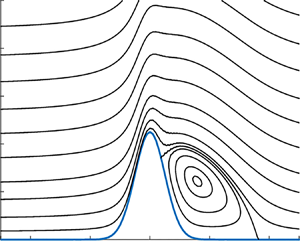
The graphic illustration of this solution is presented in figure 2.

Figure 2. The real (bold line) and imaginary (dashed line) parts of function $\breve {h}_1$ calculated for $x = 1$, $\alpha = 1$ and two values of the Mach number, $M_{\infty } = 0.5$ and $0.9$.

With known $h_1$ we can use the state (2.2c) to find the density perturbations in the transition layer. We have

(5.30)\begin{equation} \rho _1 ={-} (\gamma - 1) M_{\infty }^2 h_1 = \frac{{\rm \pi} \textrm{i}}{2} \, \textrm{e}^{\textrm{i} \alpha \xi } z H_1^{(1)} (z) + (\textrm{c.c.}) . \end{equation}

Now we can return to the continuity equation (5.17). To avoid a degeneration in this equation, we need to choose $\sigma$ according to (5.21), that is

(5.31)\begin{equation} \sigma = Re^{{-}1/2} \frac{\varepsilon }{\delta } , \end{equation}

and then the continuity equation assumes the form

(5.32)\begin{equation} \frac{\partial v_1}{\partial \bar{Y}} = \textrm{e}^{-\bar{Y} / \sqrt{x}} \frac{\partial \rho _1}{\partial \xi } + \frac{1}{\sqrt{x}} \frac{\partial \rho _1} {\partial \bar{Y}} . \end{equation}

It has to be integrated with the disturbance attenuation condition (5.12b)

(5.33)\begin{equation} v_1 = 0 \quad \text{at} \ \bar{Y} ={-}\infty . \end{equation}

We shall leave this task for others to perform.

6. Triple-deck region

The generation of Tollmien–Schlichting waves takes place as a result of the interaction of the entropy waves with steady flow perturbations caused by a wall roughness. We have chosen the frequency of the entropy waves to be $\omega = O (Re^{1/4})$. This is to satisfy the resonance condition. The second resonance condition requires the roughness size $\Delta x$ to be comparable to the wavelength of the Tollmien–Schlichting wave, that is $\Delta x = O (Re^{-3/8})$. It is well known that the flow past a roughness of this size is described by the triple-deck theory. According to this theory, when analysing the flow in the vicinity of the roughness one has to consider three regions: the viscous sublayer (region 3 in figure 3), the main part of the boundary layer (region 2) and in the upper region 1 that lies in the inviscid flow outside the boundary layer.

Figure 3. The flow in the vicinity of the wall roughness.

In this section our task is to derive the equations that describe the flow in the three layers. When performing this task we shall assume the roughness shape can be represented by the equation

(6.1)\begin{equation} y = Re^{{-}5/8} F \left( \frac{x - 1}{Re^{{-}3/8}} \right) . \end{equation}

6.1. Upper tier

In order to predict the form of asymptotic expansions of fluid-dynamic functions in the upper tier of the triple-deck region, we return to the solution (4.11a,b) for the inviscid flow upstream of the roughness. Substituting (4.7a–c) into (4.9) and then into (4.11a,b), we see that near the roughness, the solution for the entropy wave may be written in the form

(6.2)\begin{equation} \left. \begin{gathered} u = 1 + \varepsilon \cdot 0 , \quad v = \varepsilon \cdot 0 , \quad p = \varepsilon \cdot 0 , \\ \rho = 1 + \varepsilon \rho _0^{\prime } (\bar{t}\,) , \quad h = \frac{1} {(\gamma - 1) M_{\infty }^2} + \varepsilon h_0^{\prime } (\bar{t}\,) , \end{gathered} \right\} \end{equation}

where

(6.3a,b)\begin{equation} \rho _0^{\prime } (\bar{t}\,) = \rho _{\alpha } \textrm{e}^{\textrm{i} \omega \bar{t}} + (\textrm{c.c.}) , \quad h_0^{\prime } (\bar{t}\,) = h_{\alpha } \textrm{e}^{\textrm{i} \omega \bar{t}} + (\textrm{c.c.}) . \end{equation}

The frequency of oscillations $\omega$ coincides with the wavenumber $\alpha$ of the entropy wave, and the amplitude is given by

(6.4a,b)\begin{equation} \rho _{\alpha } = \textrm{e}^{- \textrm{i} \alpha \bar{x}_0} , \quad h_{\alpha } ={-} \frac{\textrm{e}^{- \textrm{i} \alpha \bar{x}_0}}{(\gamma - 1) M_{\infty }^2} , \end{equation}

where $\bar {x}_0$ denoting the value of $\bar {x}$ at the position of the roughness.

Keeping further in mind that the wall roughness (6.1) produces $O (Re^{-1/4})$ steady perturbations in the flow, we represent the fluid-dynamic functions in the upper tier in the form

(6.5)\begin{equation} \left. \begin{aligned} u & = 1 + Re^{{-}1/4} u_1^{{\ast} } (x_{{\ast} } , y_{{\ast} }) + \varepsilon Re^{{-}1/4} u_2^{{\ast} } (\bar{t} , x_{{\ast} } , y_{{\ast} }) + \cdots ,\\ v & = Re^{{-}1/4} v_1^{{\ast} } (x_{{\ast} } , y_{{\ast} }) + \varepsilon Re^{{-}1/4} v_2^{{\ast} } (\bar{t} , x_{{\ast} } , y_{{\ast} }) + \cdots ,\\ p & = Re^{{-}1/4} p_1^{{\ast} } (x_{{\ast} } , y_{{\ast} }) + \varepsilon Re^{{-}1/4} p_2^{{\ast} } (\bar{t} , x_{{\ast} } , y_{{\ast} }) + \cdots ,\\ \rho & = 1 + \varepsilon \rho _0^{\prime } (\bar{t}\,) + Re^{{-}1/4} \rho_1^{{\ast} } (x_{{\ast} } , y_{{\ast} }) + \varepsilon Re^{{-}1/4} \rho _2^{{\ast} } (\bar{t} , x_{{\ast} } , y_{{\ast} }) + \cdots ,\\ h & = \frac{1}{(\gamma - 1) M_{\infty }^2} + \varepsilon h_0^{\prime } (\bar{t}\,) + Re^{{-}1/4} h_1^{{\ast} } (x_{{\ast} } , y_{{\ast} }) + \varepsilon Re^{{-}1/4} h_2^{{\ast} } (\bar{t} , x_{{\ast} } , y_{{\ast} }) + \cdots , \end{aligned} \right\} \end{equation}

with the independent variables being

(6.6a–c)\begin{equation} \bar{t} = \frac{t}{Re^{{-}1/4}} , \quad x_{{\ast} } = \frac{x - 1}{Re^{{-}3/8}} , \quad y_{{\ast} } = \frac{y}{Re^{{-}3/8}} . \end{equation}

The $O (\varepsilon Re^{-1/4})$ terms in (6.5) represent the perturbations produced by the interaction of the unsteady perturbations in the entropy wave with the steady caused by the wall roughness.

The equations for the $O (Re^{-1/4})$ and $O (\varepsilon Re^{-1/4})$ terms are obtained by substituting (6.5), (6.6a–c) into the Navier–Stokes equations (2.2). The perturbations produced by the wall roughness are governed by the linearised Euler equations

(6.7)\begin{equation} \left. \begin{gathered} \frac{\partial u_1^{{\ast} }}{\partial x_{{\ast} }} ={-} \frac{\partial p_1^{{\ast} }} {\partial x_{{\ast} }} , \quad \frac{\partial v_1^{{\ast} }}{\partial x_{{\ast} }} ={-} \frac{\partial p_1^{{\ast} }} {\partial y_{{\ast} }} , \quad \frac{\partial h_1^{{\ast} }}{\partial x_{{\ast} }} = \frac{\partial p_1^{{\ast} }} {\partial x_{{\ast} }} , \\ \frac{\partial u_1^{{\ast} }}{\partial x_{{\ast} }} + \frac{\partial \rho_1^{{\ast} }} {\partial x_{{\ast} }} + \frac{\partial v_1^{{\ast} }}{\partial y_{{\ast} }} = 0, \quad h_1^{{\ast} } =\frac{\gamma}{\gamma - 1} p_1^{{\ast} } - \frac{1}{(\gamma - 1) M_{\infty}^{2}} \rho_1^{{\ast} }. \end{gathered} \right\} \end{equation}

These equations were encountered on numerous occasions before in the context of the triple-deck theory; see § 4.2.3 in Ruban (Reference Ruban2018). They may be reduced, by means of elimination, to a single equation for the pressure $p_1^{\ast }$

(6.8)\begin{equation} (1 - M_{\infty }^2) \frac{\partial p_1^{{\ast} }}{\partial x_{{\ast} }^2} + \frac{\partial p_1^{{\ast} }}{\partial y_{{\ast} }^2} = 0 . \end{equation}

With known $p_1^{\ast }$ the enthalpy $h_1^{\ast }$, longitudinal velocity $u_1^{\ast }$ and density $\rho _1^{\ast }$ are calculated as

(6.9a–c)\begin{equation} h_1^{{\ast} } = p_1^{{\ast} } , \quad u_1^{{\ast} } ={-} p_1^{{\ast} } , \quad \rho _1^{{\ast} } = M_{\infty }^2 p_1^{{\ast} } . \end{equation}

The equations for the $O (\varepsilon Re^{-1/4})$ terms are found to be

(6.10a)$$\begin{gather} \frac{\partial u_2^{{\ast} }}{\partial x_{{\ast} }} + \frac{\partial p_2^{{\ast} }} {\partial x_{{\ast} }} ={-}\rho_0^{\prime } (\bar{t}\,) \frac{\partial u_1^{{\ast} }} {\partial x_{{\ast} }}, \end{gather}$$

(6.10b)$$\begin{gather}\frac{\partial v_2^{{\ast} }}{\partial x_{{\ast} }} + \frac{\partial p_2^{{\ast} }} {\partial y_{{\ast} }} ={-}\rho_0^{\prime } (\bar{t}\,) \frac{\partial v_1^{{\ast} }} {\partial x_{{\ast} }}, \end{gather}$$

(6.10c)$$\begin{gather}\frac{\partial h_2^{{\ast} }}{\partial x_{{\ast} }} - \frac{\partial p_2^{{\ast} }} {\partial x_{{\ast} }} ={-}\rho_0^{\prime } (\bar{t}\,) \frac{\partial h_1^{{\ast} }} {\partial x_{{\ast} }} , \end{gather}$$

(6.10d)$$\begin{gather}\frac{\partial u_2^{{\ast} }}{\partial x_{{\ast} }} + \frac{\partial \rho_2^{{\ast} }} {\partial x_{{\ast} }} + \frac{\partial v_2^{{\ast} }}{\partial y_{{\ast} }} ={-}\rho_{0}^{\prime } (\bar{t}\,) \left( \frac{\partial u_1^{{\ast} }} {\partial x_{{\ast} }} + \frac{\partial v_1^{{\ast} }}{\partial y_{{\ast} }} \right), \end{gather}$$

(6.10e)$$\begin{gather}h_2^{{\ast} } =\frac{\gamma}{\gamma - 1} p_2^{{\ast} } - \frac{1}{(\gamma - 1) M_{\infty }^2}\rho _2^{{\ast} } + \frac{2 - \gamma}{\gamma - 1} \rho_{0}^{\prime} (\bar{t}\,) p_1^{{\ast} } . \end{gather}$$

Performing the elimination routine again we find that the pressure $p_2^{\ast }$ satisfies the following equation:

(6.11)\begin{equation} (1 - M_{\infty}^{2}) \frac{\partial ^2 p_2^{{\ast} }}{\partial x_{{\ast} }^2} + \frac{\partial ^2 p_2^{{\ast} }}{\partial y_{{\ast} }^2} = \rho_0^{\prime} (\bar{t}\,) M_{\infty}^2 \frac{\partial ^2 p_1^{{\ast} }}{\partial x_{{\ast} }^2} . \end{equation}

Before formulating the boundary conditions for (6.8) and (6.11) we need to consider the lower and middle tiers in the triple-deck structure (see figure 3).

6.2. Lower tier

Since the pressure does not change across the boundary layer, its asymptotic representation in the lower tier should be the same as in the upper tier; see the expansion for $p$ in (6.5). Correspondingly, we shall seek the solution of the Navier–Stokes equations (2.2) in the lower tier in the form

(6.12)\begin{equation} \left. \begin{aligned} u & = Re^{{-}1/8} U_1^{{\ast} }(x_{{\ast} } , Y_{{\ast} }) + \varepsilon Re^{{-}1/8} U_2^{{\ast} } (\bar{t} , x_{{\ast} } , Y_{{\ast} }) + \cdots , \\ v & = Re^{{-}3/8} V_1^{{\ast} } (x_{{\ast} } , Y_{{\ast} }) + \varepsilon Re^{{-}3/8} V_2^{{\ast} } (\bar{t} , x_{{\ast} } , Y_{{\ast} }) + \cdots , \\ p & = Re^{{-}1/4} P_1^{{\ast} } (x_{{\ast} }, Y_{{\ast} }) + \varepsilon Re^{{-}1/4} P_2^{{\ast} } (\bar{t} , x_{{\ast} } , Y_{{\ast} }) + \cdots , \\ \rho & = \rho_w + \cdots, \quad h = h_w + \cdots , \quad \mu = \mu _w + \cdots . \end{aligned} \right\} \end{equation}

Here, the scaled time $\bar {t}$ and longitudinal coordinate $x_{\ast }$ are the same (6.6a–c) as in the upper tier, while the lateral coordinate $Y_{\ast }$ is introduced as

(6.13)\begin{equation} Y_{{\ast} } = \frac{y}{Re^{{-}5/8}} . \end{equation}

Since the flow in the lower tier is slow, it may be treated as incompressible with the density, enthalpy and viscosity coefficient being constant. We denote their values as $\rho _w$, $h_w$ and $\mu _w$, respectively. These are obtained from the solution of the boundary-layer equations at the position of the roughness

(6.14a–c)\begin{equation} \rho _w = \rho _0 (1 , 0) , \quad h_w = h_0 (1 , 0) , \quad \mu _w = \mu _0 (1 , 0) . \end{equation}

Substitution of (6.12) into the Navier–Stokes equations (2.2) yields in the leading-order approximation

(6.15a)$$\begin{gather} \rho _w \left( U_1^{{\ast} } \frac{\partial U_1^{{\ast} }}{\partial x_{{\ast} }} + V_1^{{\ast} } \frac{\partial U_1^{{\ast} }}{\partial Y_{{\ast} }} \right) ={-} \frac{\partial P_1^{{\ast} }}{\partial x_{{\ast} }} + \mu _w \frac{\partial ^2 U_1^{{\ast} }}{\partial Y_{{\ast} }^2}, \end{gather}$$

(6.15b)$$\begin{gather}\frac{\partial P_1^{{\ast} }}{\partial Y_{{\ast} }} = 0, \end{gather}$$

(6.15c)$$\begin{gather}\frac{\partial U_1^{{\ast} }}{\partial x_{{\ast} }} + \frac{\partial V_1^{{\ast} }} {\partial Y_{{\ast} }} = 0 . \end{gather}$$

These are conventional incompressible steady flow boundary-layer equations. They have to be solved with the no-slip conditions on the surface of the roughness (6.1)

(6.16)\begin{equation} U_1^{{\ast} } = V_1^{{\ast} } = 0 \quad \text{at} \ Y_{{\ast} } = F (x_{{\ast} }) , \end{equation}

and the following condition of matching with the solution in the boundary layer upstream of the roughness:

(6.17)\begin{equation} U_1^{{\ast} } = \lambda Y_{{\ast} } \quad \text{at} \ x_{{\ast} } ={-} \infty , \end{equation}

where $\lambda$ is dimensionless skin friction given by

(6.18)\begin{equation} \lambda = \left.\frac{\partial U_0}{\partial Y}\right|_{x=1,\,Y=0} . \end{equation}

It may be shown (see § 2.2.4 in Ruban Reference Ruban2018) that the solution to (6.15) satisfying condition (6.17) exhibits the following behaviour at the outer edge of the lower tier:

(6.19)\begin{equation} U_1^{{\ast} } = \lambda Y_{{\ast} } + A_1^{{\ast} } (x_{{\ast} }) + \cdots , \quad V_1^{{\ast} } ={-} \frac{\textrm{d} A_1^{{\ast} }}{\textrm{d}\kern0.06em x_{{\ast} }} Y_{{\ast} } + \cdots \quad \text{as} \ Y_{{\ast} } \to \infty , \end{equation}

where $A_1^{\ast } (x_{\ast })$ is termed the displacement function.

Now, turning to the second-order terms in (6.12), we have to consider the equations

(6.20a)$$\begin{gather} \rho _w \left( \frac{\partial U_2^{{\ast} }}{\partial \bar{t}} + U_1^{{\ast} } \frac{\partial U_2^{{\ast} }}{\partial x_{{\ast} }} + U_2^{{\ast} }\frac{\partial U_1^{{\ast} }}{\partial x_{{\ast} }} + V_1^{{\ast} } \frac{\partial U_2^{{\ast} }} {\partial Y_{{\ast} }} + V_2^{{\ast} } \frac{\partial U_1^{{\ast} }}{\partial Y_{{\ast} }} \right) ={-} \frac{\partial P_2^{{\ast} }}{\partial x_{{\ast} }} + \mu_w \frac{\partial ^2 U_2^{{\ast} }}{\partial Y_{{\ast} }^2}, \end{gather}$$

(6.20b)$$\begin{gather}\frac{\partial P_2^{{\ast} }}{\partial Y_{{\ast} }} = 0, \end{gather}$$

(6.20c)$$\begin{gather}\frac{\partial U_2^{{\ast} }}{\partial x_{{\ast} }} + \frac{\partial V_2^{{\ast} }} {\partial Y_{{\ast} }} =0 . \end{gather}$$

They have to be solved subject of the no-slip conditions on the surface of the roughness

(6.21)\begin{equation} U_2^{{\ast} } = V_2^{{\ast} } = 0 \quad \text{at} \ Y_{{\ast} } = F (x_{{\ast} }) , \end{equation}

and the matching condition with the solution in the boundary layer upstream of the roughness

(6.22)\begin{equation} U_2^{{\ast} } \to 0 \quad \text{as} \ x_{{\ast} } \to -\infty. \end{equation}

Again, it may be shown that at the outer edge of the lower tier

(6.23)\begin{equation} U_2^{{\ast} } = A_2^{{\ast} } (\bar{t} , x_{{\ast} }) + \cdots , \quad V_2^{{\ast} } ={-} \frac{\partial A_2^{{\ast} }}{\partial x_{{\ast} }} Y_{{\ast} } + \cdots \quad \text{as} \ Y_{{\ast} } \to \infty . \end{equation}

6.3. Middle tier

Region 2, the middle tier (see figure 3), represents a continuation of the conventional boundary layer into the triple-deck region. The thickness of region 2 is estimated as $y \sim Re^{-1/2}$. Consequently, the asymptotic analysis of the Navier–Stokes equations (2.2) in region 2 has to be performed based on the limit

(6.24a–d)\begin{equation} \bar{t} = \frac{t}{Re^{{-}1/4}} , \quad x_{{\ast} } = \frac{x - 1}{Re^{{-}3/8}} = O(1) , \quad Y = \frac{y}{Re^{{-}1/2}} = O(1) , \quad Re \to \infty . \end{equation}

The form of the asymptotic expansions of the fluid-dynamic functions in region 2 may be predicted by analysing the solution in the overlap region that lies between regions 3 and 2. Let us examine the velocity components. In region 3, they are represented in the form of asymptotic expansions (6.12). At the outer edge of region 3, the coefficients in these expansions behave as described by (6.19) and (6.23). If we substitute (6.19), (6.23) into (6.12) and express the resulting equations in terms of variables of region 2, that is, perform the substitution $Y_{\ast } = Re^{1/8} Y$, then we will find that at the ‘bottom’ of region 2

(6.25)\begin{equation} \left. \begin{aligned} u & = \lambda Y + Re^{{-}1/8} A_1^{{\ast} } (x_{{\ast} }) + \varepsilon Re^{{-}1/8} A_2^{{\ast} } (\bar{t} , x_{{\ast} }) + \cdots , \\ v & = Re^{{-}1/4} \left( - \frac{\textrm{d} A_1^{{\ast} }}{\textrm{d}\kern0.06em x_{{\ast} }} Y \right) + \varepsilon Re^{{-}1/4} \left( - \frac{\partial A_2^{{\ast} }}{\partial x_{{\ast} }} Y \right) +\cdots . \end{aligned} \right\} \end{equation}

This suggests that the solution in region 2 should be sought in the form

(6.26)\begin{equation} \left. \begin{aligned} u & = U_{00} (Y) + Re^{{-}1/8} \tilde{U}_1 (x_{{\ast} } , Y) + \varepsilon Re^{{-}1/8} \tilde{U}_2 (\bar{t} , x_{{\ast} } , Y) + \cdots , \\ v & = Re^{{-}1/4} \tilde{V}_1 (x_{{\ast} } , Y) + \varepsilon Re^{{-}1/4} \tilde{V}_2 (\bar{t} , x_{{\ast} } , Y) + \cdots . \end{aligned} \right\} \end{equation}

The leading-order term $U_{00} (Y)$ in the expansion for $u$ coincides with the velocity profile in the boundary layer immediately before the triple-deck region. According to (3.7)

(6.27)\begin{equation} U_{00} = \lambda Y + \cdots \quad \text{as} \ Y \to 0 . \end{equation}

It further follows from (6.25) that the perturbation terms $\tilde {U}_1 (x_{\ast } , Y)$, $\tilde {U}_2 (\bar {t} , x_{\ast } , Y)$, $\tilde {V}_1 (x_{\ast } , Y)$ and $\tilde {V}_2 (\bar {t} , x_{\ast } , Y)$ in (6.26) should exhibit the following behaviour at the ‘bottom’ of region 2:

(6.28)\begin{equation} \tilde{U}_1= A_1^{{\ast} } (x_{{\ast} }) + \cdots ,\quad \tilde{V}_1 ={-} \frac{\textrm{d} A_1^{{\ast} }}{\textrm{d}\kern0.06em x_{{\ast} }} Y + \cdots \quad \text{as} \ Y \to 0 , \end{equation}

and

(6.29)\begin{equation} \tilde{U}_2 = A_2^{{\ast} } (\bar{t} , x_{{\ast} }) + \cdots ,\quad \tilde{V}_2 ={-} \frac{\partial A_2^{{\ast} }}{\partial x_{{\ast} }} Y + \cdots \quad \text{as} \ Y \to 0 . \end{equation}

By analogy with the longitudinal velocity component $u$ in (6.26), we shall seek the enthalpy $h$, the density $\rho$ and the viscosity $\mu$ in region 2 in the form of the asymptotic expansions

(6.30)\begin{equation} \left. \begin{aligned} h & = h_{00} (Y) + Re^{{-}1/8} \tilde{h}_1 (x_{{\ast} } , Y) + \varepsilon Re^{{-}1/8} \tilde{h}_2 (\bar{t} , x_{{\ast} } , Y) + \cdots , \\ \rho & = \rho _{00} (Y) + Re^{{-}1/8} \tilde{\rho }_1 (x_{{\ast} } , Y) + \varepsilon Re^{{-}1/8} \tilde{\rho }_2 (\bar{t} , x_{{\ast} } , Y) + \cdots , \\ \mu & = \mu _{00} (Y) + Re^{{-}1/8} \tilde{\mu }_1 (x_{{\ast} } , Y) + \varepsilon Re^{{-}1/8} \tilde{\mu }_2 (\bar{t} , x_{{\ast} } , Y) + \cdots . \end{aligned} \right\} \end{equation}

Finally, we expect the pressure $p$ to remain unchanged across the boundary layer. Consequently, the asymptotic representation of $p$ in region 2 should have the same form

(6.31)\begin{equation} p = Re^{{-}1/4} \tilde{P}_1 (x_{{\ast} } , Y) + \varepsilon Re^{{-}1/4} \tilde{P}_2 (\bar{t} , x_{{\ast} } , Y) + \cdots \end{equation}

as that in region 3; see (6.12).

The substitution of (6.26), (6.30) and (6.31) into the Navier–Stokes equations (2.2) results in

(6.32)\begin{equation} \left. \begin{gathered} U_{00} (Y)\,\frac {\partial \tilde{U}_1}{\partial x_{{\ast} }} + \tilde{V}_1 \frac{\textrm{d} U_{00}}{\textrm{d} Y} = 0 , \\ \frac {\partial \tilde{P}_1}{\partial Y} = 0 , \\ U_{00} (Y)\,\frac {\partial \tilde{h}_1}{\partial x_{{\ast} }} + \tilde{V}_1 \frac{\textrm{d} h_{00}}{\textrm{d} Y} = 0 , \\ \rho _{00} (Y) \frac {\partial \tilde{U}_1}{\partial x_{{\ast} }} + U_{00} (Y) \frac {\partial \tilde{\rho }_1}{\partial x_{{\ast} }} + \rho _{00} (Y) \frac {\partial \tilde{V}_1}{\partial Y} + \tilde{V}_1 \frac{\textrm{d} \rho _{00}}{\textrm{d} Y} = 0 , \\ h_{00} = \frac{1}{(\gamma - 1) M_{\infty }^2}\,\frac{1}{\rho _{00}} , \quad \tilde{h}_1 ={-} \frac{1}{(\gamma - 1) M_{\infty }^2}\, \frac{\tilde{\rho }_1}{\rho _{00}^2} . \end{gathered} \right\} \end{equation}

The solution to (6.32) satisfying boundary conditions (6.28) is

(6.33a,b)\begin{equation} \tilde{U}_1 = \frac{1}{\lambda } A_1^{{\ast} } (x_{{\ast} }) U_{00}^{\prime } (Y) , \quad \tilde{V}_1 ={-} \frac{1}{\lambda } \frac{\textrm{d} A_1^{{\ast} }}{\textrm{d}\kern0.06em x_{{\ast} }} U_{00} (Y) . \end{equation}

The unsteady perturbation terms are analysed in the same way, leading to a conclusion that in the middle tier

(6.34a,b)\begin{equation} \tilde{U}_2 = \frac{1}{\lambda } A_2^{{\ast} } (\bar{t} , x_{{\ast} }) U_{00}^{\prime } (Y) , \quad \tilde{V}_2 ={-} \frac{1}{\lambda } \frac{\partial A_2^{{\ast} }}{\partial x_{{\ast} }} U_{00} (Y) . \end{equation}

7. Viscous–inviscid interaction problem

We are now ready to formulate the boundary conditions for (6.8) and (6.11) in the upper tier. For this purpose we shall perform the matching of the streamline slope angle $\vartheta$ in regions 2 and 1. Using (6.26) we can calculate $\vartheta$ in region 2 (the middle tier) as

(7.1)\begin{equation} \vartheta = \arctan \frac{v}{u} = Re^{{-}1/4} \frac{\tilde{V}_1}{U_{00}} + \varepsilon Re^{{-}1/4} \frac{\tilde{V}_2}{U_{00}} + \cdots . \end{equation}

It then follows from (6.33a,b), (6.34a,b) that

(7.2)\begin{equation} \vartheta = Re^{{-}1/4} \left( - \frac{1}{\lambda } \frac{\textrm{d} A_1^{{\ast} }}{\textrm{d}\kern0.06em x_{{\ast} }} \right) + \varepsilon Re^{{-}1/4} \left( - \frac{1}{\lambda } \frac{\partial A_2^{{\ast} }} {\partial x_{{\ast} }} \right) + \cdots . \end{equation}

To calculate $\vartheta$ in the upper tier, we have to use the asymptotic expansions of $u$ and $v$ given by (6.5). We have

(7.3)\begin{equation} \vartheta = \arctan \frac{v}{u} = Re^{{-}1/4} v_1^{{\ast} } (x_{{\ast} } , y_{{\ast} }) + \varepsilon Re^{{-}1/4} v_2^{{\ast} } (\bar{t} , x_{{\ast} } , y_{{\ast} }) + \cdots . \end{equation}

We now need to set $y_{\ast } \to 0$ in (7.3) and compare (7.3) with (7.2). We see that

(7.4a,b)\begin{equation} \left. v_1^{{\ast} }\right|_{y_{{\ast} } = 0} ={-} \frac{1}{\lambda } \frac{\textrm{d} A_1^{{\ast} }} {\textrm{d}\kern0.06em x_{{\ast} }} , \quad \left. v_2^{{\ast} }\right|_{y_{{\ast} } = 0} ={-} \frac{1}{\lambda } \frac{\partial A_2^{{\ast} }}{\partial x_{{\ast} }} . \end{equation}

Conditions (7.4a,b) are easily converted into conditions for the pressure. This is done by setting $y_{\ast } = 0$ in the second equation in (6.7) and in (6.10b). We have

(7.5a,b)\begin{equation} \left. \frac{\partial p_1^{{\ast} }}{\partial y_{{\ast} }}\right|_{y_{{\ast} } = 0} = \frac{1}{\lambda } \frac{\textrm{d}^2 A_1^{{\ast} }}{\textrm{d}\kern0.06em x_{{\ast} }^2} , \quad \left. \frac{\partial p_2^{{\ast} }}{\partial y_{{\ast} }}\right|_{y_{{\ast} } = 0} = \frac{1}{\lambda } \frac{\partial ^2 A_2^{{\ast} }}{\partial x_{{\ast} }^2} + \frac{1}{\lambda } \rho _0^{\prime } (\bar{t}) \frac{\textrm{d}^2 A_1^{{\ast} }} {\textrm{d}\kern0.06em x_{{\ast} }^2} . \end{equation}

To complete the formulation of the boundary-value problem in the upper tier one needs to supplement (7.5a,b) with perturbation attenuation conditions

(7.6)\begin{equation} p_1^{{\ast} } \to 0 , \quad p_2^{{\ast} } \to 0 \quad \text{as} \ x_{{\ast} }^2 + y_{{\ast} }^2 \to \infty . \end{equation}

7.1. Steady flow

To describe the steady perturbations produced in the flow by the wall roughness we need to analyse the flow in the lower tier simultaneously with the flow in the upper tier as these are in mutual interaction with one another. In the lower tier we have to solve (6.15) subject to the boundary conditions (6.16)–(6.19). In the upper tier the flow is governed by equation (6.8) which should be solved with the boundary conditions on $p_1^{\ast }$ in (7.5a,b) and (7.6). Considered together these equations and boundary conditions constitute the steady viscous–inviscid interaction problem. This problem involves four parameters: the dimensionless skin friction immediately before the interaction region $\lambda$, the fluid density $\rho _w$ and viscosity coefficient $\mu _w$ on the body surface and the ‘compressibility’ parameter $\beta = \sqrt {1 - M_{\infty }^2}$. We perform the substitution of variables

(7.7)\begin{equation} \left. \begin{aligned} x_{{\ast} } & = \frac{\mu _w^{{-}1/4} \rho _w^{{-}1/2}} {\lambda ^{5/4} \beta ^{3/4}} \,\bar{X} , \quad Y_{{\ast} } = \frac{\mu _w^{1/4} \rho _w^{{-}1/2}}{\lambda ^{3/4} \beta ^{1/4}} \, \bar{Y} + F (x_{{\ast} }) , \\ U_1^{{\ast} } & = \frac{\mu _w^{1/4} \rho _w^{{-}1/2}}{\lambda ^{{-}1/4} \beta ^{1/4}} \,\bar{U}_1 , \quad V_1^{{\ast} } = \frac{\mu _w^{3/4} \rho _w^{{-}1/2}}{\lambda ^{{-}3/4} \beta ^{{-}1/4}} \, \bar{V}_1 + U_1^{{\ast} } \frac{\textrm{d} F}{\textrm{d}\kern0.06em x_{{\ast} }}, \\ P_1^{{\ast} } & = \frac{\mu _w^{1/2}}{\lambda ^{{-}1/2} \beta ^{1/2}} \,\bar{P}_1 , \quad A_1^{{\ast} } = \frac{\mu _w^{1/4} \rho _w^{{-}1/2}}{\lambda ^{{-}1/4} \beta ^{1/4}} \, \bar{A}_1 - \lambda F (x_{{\ast} }) , \end{aligned} \right\} \end{equation}

that combines standard affine transformations of the triple-deck theory with Prandtl's transposition. The latter introduces the body-fitted coordinates $(\bar {X} , \bar {Y})$ with $\bar {X}$ measured along the roughness contour and $\bar {Y}$ in the normal direction. Here, it is assumed that the roughness shape function can be expressed in the form

(7.8)\begin{equation} F = \frac{\mu _w^{1/4} \rho _w^{{-}1/2}}{\lambda ^{3/4} \beta ^{1/4}} \, \bar{F} , \end{equation}

where $\bar {F} (\bar {X})$ is independent of $\lambda$, $\rho _w$, $\mu _w$ and $\beta$.

As a result of transformations (7.7) equations (6.15) and boundary conditions (6.16)–(6.19) assume that form

(7.9)\begin{equation} \left. \begin{gathered} \bar{U}_1 \frac{\partial \bar{U}_1}{\partial \bar{X}} + \bar{V}_1 \frac{\partial \bar{U}_1}{\partial \bar{Y}} ={-} \frac{\textrm{d} \bar{P}_1}{\textrm{d} \bar{X}} + \frac{\partial ^2 \bar{U}_1}{\partial \bar{Y}^2} ,\\ \frac{\partial \bar{U}_1}{\partial \bar{X}} + \frac{\partial \bar{V}_1} {\partial \bar{Y}} = 0 ,\\ \bar{U}_1 = \bar{V}_1 = 0 \quad \text{at} \ \bar{Y} = 0 ,\\ \bar{U}_1 = \bar{Y} + \cdots \quad \text{as} \ \bar{X} \to - \infty ,\\ \bar{U}_1 = \bar{Y} + \bar{A}_1 (\bar{X}) + \cdots \quad \text{as} \ \bar{Y} \to \infty . \end{gathered} \right\} \end{equation}

Corresponding to (7.7) the upper tier variables are transformed as

(7.10a,b)\begin{equation} y_{{\ast} } = \frac{\mu _w^{{-}1/4} \rho _w^{{-}1/2}}{\lambda ^{5/4} \beta^{7/4}} \bar{y}, \quad p_1^{{\ast} } = \frac{\mu _w^{1/2}}{\lambda ^{{-}1/2} \beta^{1/2}} \bar{p}_1. \end{equation}

This turns equation (6.8) and boundary conditions for $p_1^{\ast }$ in (7.5a,b) and (7.6) into

(7.11)\begin{equation} \left. \begin{gathered} \frac{\partial ^2 \bar{p}_1}{\partial \bar{X}^2} + \frac{\partial ^2 \bar{p}_1} {\partial \bar{y}^2} = 0,\\ \left. \frac{\partial \bar{p}_1}{\partial \bar{y}}\right|_{\bar{y}=0} = \frac {\textrm{d}^{2} \bar{A}_1}{\textrm{d} \bar{X}^2} - \frac {\textrm{d}^2 \bar{F}}{\textrm{d} \bar{X}^2} , \\ \bar{p}_1 \to 0 \quad \text{as} \ \bar{X}^2 + \bar{y}^2 \to \infty . \end{gathered} \right\} \end{equation}

7.2. Unsteady perturbations

To study the unsteady perturbations we need to consider (6.20) in the lower tier. These should be solved subject to boundary conditions (6.21)–(6.23). The transformations

(7.12)\begin{equation} \left. \begin{gathered} \bar{t} = \frac{\mu _w^{{-}1/2}}{\lambda ^{3/2} \beta^{1/2}} T , \quad \omega =\frac{\mu _w^{1/2}}{\lambda ^{{-}3/2} \beta ^{{-}1/2}} \bar{\omega } ,\\ U_2^{{\ast} } = \frac{\mu _w^{1/4} \rho _w^{{-}1/2}}{\lambda ^{{-}1/4} \beta ^{1/4}} \bar{U}_2 , \quad V_2^{{\ast} } = \frac{\mu _w^{3/4} \rho _w^{{-}1/2}} {\lambda ^{{-}3/4} \beta^{{-}1/4}} \bar{V}_2 + U_2^{{\ast} } \frac{\textrm{d} F}{\textrm{d}\kern0.06em x_{{\ast} }},\\ P_2^{{\ast} } = \frac{\mu _w^{1/2}}{\lambda ^{{-}1/2} \beta ^{1/2}} \bar{P}_2 , \quad A_2^{{\ast} } = \frac{\mu _w^{1/4} \rho _w^{{-}1/2}}{\lambda ^{{-}1/4} \beta^{1/4}} \bar{A}_2 \end{gathered} \right\} \end{equation}

turn (6.20)–(6.23) into

(7.13)\begin{equation} \left. \begin{gathered} \frac{\partial \bar{U}_2}{\partial T} + \bar{U}_1 \frac{\partial \bar{U}_2} {\partial \bar{X}} + \bar{U}_2 \frac{\partial \bar{U}_1}{\partial \bar{X}} + \bar{V}_1 \frac{\partial \bar{U}_2}{\partial \bar{Y}} + \bar{V}_2 \frac{\partial \bar{U}_1}{\partial \bar{Y}} ={-}\frac{\partial \bar{P}_2} {\partial \bar{X}} + \frac{\partial ^2 \bar{U}_2}{\partial \bar{Y}^2} ,\\ \frac{\partial \bar{U}_2}{\partial \bar{X}} + \frac{\partial \bar{V}_2} {\partial \bar{Y}} = 0,\\ \bar{U}_2 = \bar{V}_2 = 0 \quad \text{at} \ \bar{Y} = 0 ,\\ \bar{U}_2 = 0 \quad \text{at} \ \bar{X} ={-} \infty ,\\ \bar{U}_2 = \bar{A}_2 (T , \bar{X}) + \cdots \quad \text{as} \ \bar{Y} \to \infty . \end{gathered} \right\} \end{equation}

In the upper tier the unsteady perturbations are governed by (6.11). It should be solved subject to boundary conditions on $p_2^{\ast }$ in (7.5a,b) and (7.6). The affine transformations

(7.14a,b)\begin{equation} y_{{\ast} } = \frac{\mu _w^{{-}1/4} \rho _w^{{-}1/2}}{\lambda ^{5/4} \beta^{7/4}} \bar{y}, \quad p_2^{{\ast} } = \frac{\mu _w^{1/2}}{\lambda ^{{-}1/2} \beta ^{1/2}} \bar{p}_2 \end{equation}

turn the upper tier problem into

(7.15)\begin{equation} \left. \begin{gathered} \frac{\partial ^2 \bar{p}_2}{\partial \bar{X}^2} + \frac{\partial ^2 \bar{p}_2} {\partial \bar{y}^2} = \rho _0^{\prime} (T) \frac {M_{\infty}^2} {1 - M_{\infty}^2} \frac{\partial ^2 \bar{p}_1}{\partial \bar{X}^2} , \\ \left. \frac{\partial \bar{p}_2}{\partial \bar{y}}\right|_{\bar{y}=0} = \frac{\partial ^2 \bar{A}_2}{\partial \bar{X}^2} + \rho _0^{\prime} (T) \left( \frac {\textrm{d}^2 \bar{A}_1}{\textrm{d} \bar{X}^2} - \frac {\textrm{d}^2 \bar{F}}{\textrm{d} \bar{X}^2} \right) ,\\ \bar{p}_2 \to 0 \quad \text{as} \ \bar{X}^2 + \bar{y}^2 \to \infty . \end{gathered} \right\} \end{equation}

Here, we write $\rho _0^{\prime } (T)$ as

(7.16)\begin{equation} \rho _0^{\prime} (T) = \rho _{\alpha} \textrm{e}^{\textrm{i} \bar{\omega} T} . \end{equation}

8. Linear receptivity

Modern requirements on the quality of the surface of a passenger aircraft make typical roughness rather shallow, which allows us to write

(8.1)\begin{equation} \bar{F} = h f (\bar{X}) , \end{equation}

where $h$ is a small parameter and $f (\bar {X})$ is an order-one function.

We start with the steady flow past the roughness. In the lower tier it is described by (7.9). In the case of shallow roughness (8.1) the solution to (7.9) is sought in the form

(8.2)\begin{equation} \left. \begin{aligned} \bar{U}_1 & = \bar{Y} + h U_1 (\bar{X} , \bar{Y}) + \cdots, \quad \bar{V}_1 = h V_1 (\bar{X} , \bar{Y}) + \cdots ,\\ \bar{P}_1 & = h P_1 (\bar{X}) + \cdots, \quad \bar{A}_1 = h A_1 (\bar{X}) + \cdots . \end{aligned} \right\} \end{equation}

Functions $U_1$, $V_1$, $P_1$ and $A_1$ are found by making use of a standard routine first used by Stewartson (Reference Stewartson1970), see also § 5.1 in Ruban et al. (Reference Ruban, Bernots and Pryce2013). The solution is expressed in the form

(8.3)\begin{equation} \breve{A}_1 (k) = \frac{(\textrm{i} k)^{1/3} |k|}{(\textrm{i} k)^{1/3} |k| - 3 Ai^{\prime } (0)} \breve{f} (k) . \end{equation}

Here, $\breve {A}_1 (k)$ is the Fourier transform of the displacement function $A_1 (\bar {X})$ defined as

(8.4)\begin{equation} \breve{A}_1 (k) = \int_{-\infty }^{\infty } A_1 (\bar{X}) \textrm{e}^{-\textrm{i} k \bar{X}} \, \textrm{d} \bar{X} , \end{equation}

where $Ai^{\prime } (0)$ is the derivative of the Airy function at zero value of the argument, and $\breve {f} (k)$ is the Fourier transform of the roughness shape function $f (\bar {X})$. The solution for the pressure $p_1$ in the upper tier is expressed in terms of the Fourier transforms as

(8.5)\begin{equation} \breve{p}_1 (k , \bar{y}) = \frac{3 Ai^{\prime } (0)}{(\textrm{i} k)^{1/3} |k| - 3 Ai^{\prime } (0)} |k| \breve{f} (k) \, \textrm{e}^{-|k| \bar{y}} . \end{equation}

Now we turn to the unsteady perturbations that are governed by (7.13) and (7.15). Keeping in mind that the forcing caused by the entropy waves is periodic in time, we represent the solution in the lower tier in the form

(8.6)\begin{equation} \left. \begin{gathered} \bar{U}_2 = h \rho _{\alpha } \textrm{e}^{\textrm{i} \bar{\omega } T} U_2 (\bar{X} , \bar{Y}) + (\textrm{c.c.}) , \quad \bar{V}_2 = h \rho _{\alpha } \textrm{e}^{\textrm{i} \bar{\omega } T} V_2 (\bar{X} , \bar{Y}) + (\textrm{c.c.}) ,\\ \bar{P}_2 = h \rho _{\alpha } \textrm{e}^{\textrm{i} \bar{\omega } T} P_2 (\bar{X}) + (\textrm{c.c.}) ,\quad \bar{A}_2 = h \rho _{\alpha } \textrm{e}^{\textrm{i} \bar{\omega } T} A_2 (\bar{X}) + (\textrm{c.c.}) . \end{gathered} \right\} \end{equation}

This turns (7.13) into

(8.7)\begin{equation} \left. \begin{gathered} \textrm{i} \bar{\omega } U_2 + \bar{Y} \frac{\partial U_2}{\partial \bar{X}} + V_2 ={-} \frac{\textrm{d} P_2}{\textrm{d} \bar{X}} + \frac{\partial^2 U_2}{\partial \bar{Y}^2} ,\\ \frac{\partial U_2}{\partial \bar{X}} + \frac{\partial V_2}{\partial \bar{Y}} = 0 ,\\ U_2 = V_2 = 0 \quad \text{at} \ \bar{Y} = 0 ,\\ U_2 \to 0 \quad \text{as}\ \bar{X} \to -\infty ,\\ U_2= A_2 (\bar{X}) \quad \text{at}\ \bar{Y} = \infty . \end{gathered} \right\} \end{equation}

Correspondingly, in the upper tier the solution is sought in the form

(8.8)\begin{equation} \bar{p}_2 = h \rho _{\alpha } \textrm{e}^{\textrm{i} \bar{\omega } T} p_2 (\bar{X} , \bar{y}) + (\textrm{c.c.}) , \end{equation}

which turns (7.15) into

(8.9)\begin{equation} \left. \begin{gathered} \frac{\partial ^2 p_2}{\partial \bar{X}^2} + \frac{\partial ^2 p_2}{\partial \bar{y}^2} = \frac {M_{\infty}^2}{1 - M_{\infty}^2} \frac{\partial ^2 p_1}{\partial \bar{X}^2} , \\ \left. \frac{\partial p_2}{\partial \bar{y}}\right|_{\bar{y}=0} = \frac{\partial ^2 A_2} {\partial \bar{X}^2} + \frac {\textrm{d}^2 A_1}{\textrm{d} \bar{X}^2} - \frac {\textrm{d}^2 f}{\textrm{d} \bar{X}^2} ,\\ p_2 \to 0 \quad \text{as} \ \bar{X}^2 + \bar{y}^2 \to \infty . \end{gathered} \right\} \end{equation}

The solutions in the upper and lower tiers are linked to one another through the requirement that

(8.10)\begin{equation} P_2 = \left. p_2\right|_{\bar{y} = 0} . \end{equation}

The boundary-value problem for the upper tier (8.9) is expressed in terms of Fourier transforms as

(8.11a)$$\begin{gather} \frac{\textrm{d}^2 \breve{p}_2}{\textrm{d} \bar{y}^2} - k^2 \breve{p}_2 = \varLambda \breve{f} (k) \, \textrm{e}^{-|k| \bar{y}} , \end{gather}$$

(8.11b)$$\begin{gather}\left. \frac{\textrm{d} \breve{p}_2}{\textrm{d} \bar{y}}\right|_{\bar{y}=0} ={-} k^2 (\breve{A}_2 + \breve{A}_1 - \breve{f}) , \end{gather}$$

(8.11c)$$\begin{gather}\breve{p}_2 \to 0 \quad \text{as} \ \bar{y} \to \infty . \end{gather}$$

The forcing term on the right-hand side of (8.11a) is obtained using the solution (8.5) for $\breve {p}_1$. It is found that the constant $\varLambda$ is given by

(8.12)\begin{equation} \varLambda ={-} \frac {M_{\infty}^2}{1 - M_{\infty}^2} \frac{3 k^2 |k| Ai^{\prime} (0)} {(\textrm{i}k)^{1/3} |k| - 3 Ai^{\prime} (0)}. \end{equation}

The solution to the boundary-value problem (8.11) is written as

(8.13)\begin{equation} \breve{p}_2 = \left[ |k| (\breve{A}_2 + \breve{A}_1 - \breve{f}) - \frac{\varLambda }{2 k^2} \breve{f} (k) \right] \textrm{e}^{-|k| \bar{y}} - \frac{\varLambda } {2 |k|} \breve{f} (k) \bar{y} \textrm{e}^{- |k| \bar{y}} . \end{equation}

It remains to set $\bar {y} = 0$ and we will find that the Fourier transform of the pressure $P_2$ in the lower tier is given by

(8.14)\begin{equation} \breve{P}_2 = |k| (\breve{A}_2 + \breve{A}_1) - \left( |k| + \frac{\varLambda }{2 k^2} \right) \breve{f} (k) . \end{equation}

The equations for the lower tier (8.7) are written in terms of the Fourier transforms as

(8.15a)$$\begin{gather} \textrm{i} \bar{\omega } \breve{U}_2 + \textrm{i} k \bar{Y} \breve{U}_2 + \breve{V}_2 ={-} \textrm{i} k \breve{P}_2 + \frac{\textrm{d}^2 \breve{U}_2}{\textrm{d} \bar{Y}^2} , \end{gather}$$

(8.15b)$$\begin{gather}\textrm{i} k \breve{U}_2 + \frac{\textrm{d} \breve{V}_2}{\textrm{d} \bar{Y}} = 0 , \end{gather}$$

(8.15c)$$\begin{gather}\breve{U}_2 = \breve{V}_2 = 0 \quad \text{at} \ \bar{Y} = 0 , \end{gather}$$

(8.15d)$$\begin{gather}\breve{U}_2 = \breve{A}_2 (\bar{X}) \quad \text{at}\ \bar{Y} = \infty . \end{gather}$$

We start the solution of the boundary-value problem (8.15) by eliminating $\breve {V}_2$ from (8.15a) and (8.15b). For this purpose, we differentiate the momentum equation (8.15a) with respect to $\bar {Y}$ and then, using the continuity equation (8.15b), we find that $\breve {U}_2$ satisfies the equation

(8.16)\begin{equation} \textrm{i} (\bar{\omega } + k \bar{Y}) \frac{\textrm{d} \breve{U}_2}{\textrm{d} \bar{Y}} = \frac{\textrm{d}^3 \breve{U}_2} {\textrm{d} \bar{Y}^3} . \end{equation}

Since this is a third-order differential equation, it requires an additional boundary condition. The latter may be obtained by setting $\bar {Y} = 0$ in (8.15a). We have

(8.17)\begin{equation} \left.\frac{\textrm{d}^2 \breve{U}_2}{\textrm{d} \bar{Y}^2}\right|_{\bar{Y}=0} = \textrm{i} k \breve{P}_2 . \end{equation}

If we now introduce a new independent variable

(8.18)\begin{equation} z = z_0 + \theta \bar{Y} , \end{equation}

with

(8.19)\begin{equation} z_0 = \frac{\bar{\omega }}{k} \theta , \quad \theta = (\textrm{i} k)^{1/3} , \end{equation}

then (8.16) turns into the Airy equation for the derivative $\textrm {d} \breve {U}_2 / \textrm {d} z$

(8.20a)\begin{equation} \frac{\textrm{d}^3 \breve{U}_2}{\textrm{d} z^3} - z \frac{\textrm{d} \breve{U}_2}{\textrm{d} z} = 0 . \end{equation}

The boundary conditions (8.15c), (8.15d) and (8.17) are written in the new variables as

(8.20b)$$\begin{gather} \breve{U}_2 = 0 \quad \text{at} \ z = z_0 , \end{gather}$$

(8.20c)$$\begin{gather}\frac{\textrm{d}^2 \breve{U}_2}{\textrm{d} z^2} = (\textrm{i} k)^{1/3} \breve{P}_2 \quad \text{at} \ z = z_0 , \end{gather}$$

(8.20d)$$\begin{gather}\breve{U}_2 = \breve{A}_2 \quad \text{at}\ z = \infty . \end{gather}$$

The general solution of (8.20a) is

(8.21)\begin{equation} \frac{\textrm{d} \breve{U}_2}{\textrm{d} z} = C_1 Ai (z) + C_2 Bi (z) , \end{equation}

where $Ai (z)$ is the Airy function that decays exponentially as $z \to \infty$, while $Bi (z)$ is exponentially growing for all $k$ in the complex plane, provided that the branch cut in this plane is made along the positive imaginary semi-axis (see figure 8). It follows from (8.20d) that $\breve {U}_2$ should remain bounded. Therefore, we have to set $C_2 = 0$, and we can conclude that

(8.22)\begin{equation} \frac{\textrm{d} \breve{U}_2}{\textrm{d} z} = C_1 Ai (z) . \end{equation}

Substitution of (8.22) into (8.20c) results in

(8.23)\begin{equation} C_1 Ai^{\prime } (z_0) = (\textrm{i} k)^{1/3} \breve{P}_2 . \end{equation}

Let us now integrate (8.22) with initial condition (8.20b). We have

(8.24)\begin{equation} \breve{U}_2 = C_1 \int_{z_0}^z Ai (\zeta ) \, \textrm{d} \zeta . \end{equation}

Setting $z = \infty$ in the above equation, and using condition (8.20d) we find that

(8.25)\begin{equation} C_1 \int_{z_0}^{\infty } Ai (z) \, \textrm{d} z = \breve{A}_2 . \end{equation}

It remains to eliminate $C_1$ from (8.25) and (8.23), and we will have

(8.26)\begin{equation} \breve{A}_2 = \frac{(\textrm{i} k)^{1/3} \breve{P}_2}{Ai^{\prime } (z_0)} \int_{z_0}^{\infty } Ai (z) \, \textrm{d} z . \end{equation}

This is the second equation relating $\breve {A}_2$ and $\breve {P}_2$. The first one is given by the solution (8.14) for the upper tier. Elimination of $\breve {A}_2$ from (8.14) and (8.26) results in

(8.27)\begin{equation} \breve{P}_2 = \frac{Ai^{\prime } (z_0)}{Q (\bar{\omega } , k)} \left\{ |k| [\breve{A}_1 - \breve{f} (k)] - \frac{\Lambda }{2 k^2} \breve{f} (k) \right\} , \end{equation}

where

(8.28)\begin{equation} Q (\bar{\omega } , k) = Ai^{\prime } (z_0) - (\textrm{i} k)^{1/3} |k| \int_{z_0}^{\infty } Ai (z) \, \textrm{d} z . \end{equation}

It remains to substitute (8.3) and (8.12) into (8.27) and we arrive at a conclusion that the Fourier transform of the pressure in the lower tier is

(8.29)\begin{equation} \breve{P}_2 = \frac{Ai^{\prime } (z_0)}{Q(\bar{\omega } , k)} \left[ \frac{3 (1 + D) Ai^{\prime } (0) |k|}{(\textrm{i} k)^{1/3} |k| - 3 Ai^{\prime} (0)} \right] \breve{f} (k) , \end{equation}

where

(8.30)\begin{equation} D = \frac{M_{\infty }^2}{2 (1 - M_{\infty }^2)} . \end{equation}

To return to physical variables we need to apply the inverse Fourier transform to (8.29). Substituting the result into the equation for $\bar {P}_2$ in (8.6) we have

(8.31)\begin{equation} \bar{P}_2 (T , \bar{X}) = h \rho _{\alpha } \frac{\textrm{e}^{\textrm{i} \bar{\omega } T}}{2 {\rm \pi}} \int_{-\infty }^{\infty } \frac{Ai^{\prime } (z_0)}{Q(\bar{\omega } , k)} \left[ \frac{3 (1 + D) Ai^{\prime } (0) |k|}{(\textrm{i} k)^{1/3} |k| - 3 Ai^{\prime} (0)} \right] \breve{f} (k) \textrm{e}^{\textrm{i} k \bar{X}} \, \textrm{d} k + (\textrm{c.c.}) . \end{equation}

In the receptivity theory, our main interest is in the behaviour of the solution behind the wall roughness. The analysis presented in Appendix A shows that

(8.32)$$\begin{gather} \bar{P}_2 (T , \bar{X}) = h \rho _{\alpha } \mathcal{K} (\bar{\omega }) \breve{f} (k_1) \exp\left({\textrm{i} (k_1 \bar{X} + \bar{\omega } T)}\right) \nonumber\\ + h \rho _{\alpha } \frac {1 + D}{{\rm \pi} } \breve{f} (0) \frac {\textrm{e}^{\textrm{i} \bar{\omega } T}}{\bar{X}^2} + \cdots + (\textrm{c.c.}) \quad \text{as} \ \bar{X} \to \infty . \end{gather}$$

The Tollmien–Schlichting wave generated through the interaction of the entropy wave with a wall roughness is represented by the first term on the right-hand side of (8.32). The amplitude of the Tollmien–Schlichting wave is proportional to the receptivity coefficient $\mathcal {K} (\bar {\omega })$ and the Fourier transform $\breve {f} (k_1)$ of the roughness shape function $f (\bar {X})$ calculated for the wavenumber $k_1$ which is the wavenumber of the Tollmien–Schlichting wave for a given frequency $\bar {\omega }$ of the entropy wave. The receptivity coefficient is calculated as

(8.33)\begin{equation} \mathcal{K} (\bar{\omega }) = \left[ \frac {Ai^{\prime } (z_0)} {\partial Q / \partial k} \, \frac{3 i (1 + D) Ai^{\prime } (0) k} {(i k)^{1/3} k + 3 Ai^{\prime} (0)}\right]_{k=k_1} , \end{equation}

with $\partial Q / \partial k$ given by (A10) and $D$ by (8.30). Notice that $\mathcal {K}$ is a function of the frequency $\bar {\omega }$ and the Mach number $M_{\infty }$ only.

The numerical calculations of $\mathcal {K} (\bar {\omega })$ were performed in the following way. Firstly, a real value of the frequency $\bar {\omega }$ is chosen. The corresponding values of $k$ and $z_{0}$ are given by the first root $k_1$ of the dispersion equation (A5) which was solved with the help of Newtonian iterations. When performing the iterations, the values of the Airy function, its derivative and the integral at the point $z_0$ in the complex $z$-plane were found by solving the initial-value problem for the Airy equation along a straight line connecting the origin $z = 0$ and $z = z_0$ with the Airy function $Ai (0)$ and its derivative $Ai^{\prime } (0)$ assigned the well-known values at $z = 0$. The results of the calculations are displayed in figure 4. Notice that the argument $\phi$ of the receptivity coefficient is independent of the Mach number.

Figure 4. The receptivity coefficient $\mathcal {K} = |\mathcal {K}| \textrm {e}^{\textrm {i}\phi }$ as a function of the frequency $\bar {\omega }$ for various values of the Mach number $M_{\infty }$. (a) Modulus of the receptivity coefficient. (b) Argument of the receptivity coefficient.

9. Nonlinear receptivity

The linear receptivity analysis presented in the previous section relies on the assumption that the wall roughness is shallow, that is, the roughness shape function $\bar {F} (\bar {X})$ may be expressed in the form (8.1) with the height parameter $h$ assumed small. Under this assumption, the steady flow past the roughness is only slightly perturbed which preclude the situations when the flow involves a separation.

We shall now lift this restriction and extend the theory to the case when $\bar {F} (\bar {X})$ is an order-one quantity. In this case both the steady flow problem (7.9), (7.11) and the problem (7.13), (7.15) for unsteady perturbations require numerical solution. We used for this purpose numerical technique developed by Kravtsova, Zametaev & Ruban (Reference Kravtsova, Zametaev and Ruban2005). Some of the computation results are shown in figure 5. We chose the shape of the roughness to be $\bar {F} = h \textrm {e}^{-2 \bar {X}^2}$. Figure 5 displays the streamlines in the viscous sublayer for different values of the height parameter $h$. We found that the separation region formed when $h$ was close to $h=2.5$. The separation region increases in size as $h$ is growing.

Figure 5. Streamlines for the steady separated flow around a roughness; (a) $h=2.5$, (b) $h=3.5$, (c) $h=4.5$.

When dealing with unsteady perturbations, we modified the numerical technique of Kravtsova et al. (Reference Kravtsova, Zametaev and Ruban2005) as follows. We note that the forcing terms in (7.15), both in the equation for $\bar {p}_2$ and in the boundary condition at $\bar {y} = 0$, are periodic functions of time with frequency $\bar {\omega }$. We therefore represent the solution to (7.13) in the form

(9.1)\begin{equation} \left. \begin{aligned} \bar{U}_2 & = \rho _{\alpha } \left[ U_{21} \sin (\bar{\omega} T) + U_{22} \cos (\bar{\omega} T) \right] ,\\ \bar{V}_2 & = \rho _{\alpha } \left[ V_{21} \sin (\bar{\omega} T) + V_{22} \cos (\bar{\omega} T) \right] ,\\ \bar{P}_2 & = \rho _{\alpha } \left[ P_{21} \sin (\bar{\omega} T) + P_{22} \cos (\bar{\omega} T) \right] ,\\ \bar{A}_2 & = \rho _{\alpha } \left[ A_{21} \sin (\bar{\omega}T) + A_{22} \cos (\bar{\omega} T) \right] . \end{aligned} \right\} \end{equation}

The substitution of (9.1) into (7.13) results in the following set of linear equations:

(9.2)\begin{equation} \left. \begin{gathered} - \bar{\omega} U_{22} + \bar{U}_1 \frac{\partial U_{21}}{\partial \bar{X}} + U_{21} \frac{\partial \bar{U}_1}{\partial \bar{X}} + \bar{V}_1 \frac{\partial U_{21}} {\partial \bar{Y}} + V_{21} \frac{\partial \bar{U}_1}{\partial \bar{Y}} ={-} \frac{\partial P_{21}}{\partial \bar{X}} + \frac{\partial ^2 U_{21}}{\partial \bar{Y}^2},\\ \bar{\omega} U_{21} + \bar{U}_1 \frac{\partial U_{22}}{\partial \bar{X}} + U_{22} \frac{\partial \bar{U}_1}{\partial \bar{X}} + \bar{V}_1 \frac{\partial U_{22}} {\partial \bar{Y}} + V_{22} \frac{\partial \bar{U}_1}{\partial \bar{Y}} ={-} \frac{\partial P_{22}}{\partial \bar{X}} + \frac{\partial ^2 U_{22}}{\partial \bar{Y}^2}, \\ \frac{\partial U_{21}}{\partial \bar{X}} + \frac{\partial V_{21}}{\partial \bar{Y}} = 0, \quad \frac{\partial U_{22}}{\partial\bar{X} } + \frac{\partial V_{22}}{\partial \bar{Y}} = 0 . \end{gathered} \right\} \end{equation}

These have to be solved subject to the boundary conditions

(9.3)\begin{equation} \left. \begin{aligned} U_{21} & = U_{22} = V_{21} = V_{22} = 0 \quad \text{at} \ \bar{Y} = 0 ,\\ U_{21} & =A_{21} (\bar{X}) , \quad U_{22} =A_{22} (\bar{X}) \quad \text{at}\ \bar{Y} = \infty ,\\ U_{21} & = U_{22} = 0 \quad \text{at}\ \bar{X} ={-} \infty . \end{aligned} \right\} \end{equation}

To perform the calculations, we introduce a discrete mesh $\{\bar {X}_{i} \}$, where $i=1, \, 2, \ldots,N$, and denote the vector composed of the values of the displacement function $A (\bar {X})$ at the mesh points by $\boldsymbol {A}$, namely,

(9.4)\begin{equation} \boldsymbol{A} = \left\{ A_{21} (\bar{X}_1) ,\, A_{21} (\bar{X}_2) , \ldots , A_{21} (\bar{X}_N) , \, A_{22} (\bar{X}_1) ,\, A_{22} (\bar{X}_2) , \ldots , A_{22} (\bar{X}_N) \right\} . \end{equation}

We also consider the pressure gradient vector $\textrm {d}\boldsymbol {P}/{\textrm {d}\kern0.09em x}$ whose elements are calculated in the same way. For given displacement function $\boldsymbol {A}$, equations (9.2), (9.3) allow us to calculate the velocity field and the pressure gradient in the viscous sublayer, leading to the matrix equation

(9.5)\begin{equation} \left. \frac{\textrm{d}\boldsymbol{P}}{\textrm{d}\kern0.06em x}\right|_{{visc}} = {\boldsymbol{\mathsf{M}}} \boldsymbol{A} , \end{equation}

where ${\boldsymbol{\mathsf{M}}}$ is $2 N \times 2 N$ matrix.

The finite-difference representation of inviscid equations (7.15) can be expressed in the form

(9.6)\begin{equation} \left. \frac{\textrm{d}\boldsymbol{P}}{\textrm{d}\kern0.06em x}\right|_{{inv}} = {\boldsymbol{\mathsf{N}}} \boldsymbol{A} + \boldsymbol{R}, \end{equation}

with the vector $\boldsymbol {R}$ representing the forcing terms in (7.15).

The requirement that the pressure gradient should be the same in the viscous sublayer and at the bottom of the upper deck leads to the following set of linear equations:

(9.7)\begin{equation} ({\boldsymbol{\mathsf{M}}} - {\boldsymbol{\mathsf{N}}})\boldsymbol{A} = \boldsymbol{R}. \end{equation}

An interested reader is referred to the original paper by Kravtsova et al. (Reference Kravtsova, Zametaev and Ruban2005) for the details of numerical calculation of matrices ${\boldsymbol{\mathsf{M}}}$ and ${\boldsymbol{\mathsf{N}}}$.

The results of unsteady flow calculations at different values of the free-stream Mach number $M_{\infty }$ are shown in figure 6 in the form of the pressure gradient oscillations along the body surface. Upstream of the wall roughness the perturbations decay very fast, but they persist behind the roughness assuming the form of a Tollmien–Schlichting wave. According to the linear theory, the neutral frequency of the Tollmien–Schlichting wave is $\bar {\omega }=2.3$. Since for all values of $h$, the steady flow downstream of the roughness returns to its unperturbed state $\bar {U}_1 = \bar {Y}$, the neutral frequency $\bar {\omega }$ should not change with $h$, and figure 6 does confirm this expectation. Indeed, we see that for this frequency, the oscillations neither grow nor decay downstream of the roughness.

Figure 6. Perturbations of pressure gradient for $(\textit {a})$ $h=0.1$; $(\textit {b})$ $h=3.5$; $(\textit {c})$ $h=4.5$. In all three cases, the neutral frequency, $\bar {\omega }=2.3$, is taken.

As far as the amplitude of the oscillations is concerned, it increases rather rapidly with $h$, as figures 6(a)–6(c) clearly show. In figure 7 we show the effect of nonlinearity on the receptivity coefficient $|\mathcal {K}|$. The latter is calculated as the ratio of the amplitude of the generated Tollmien–Schlichting wave and the roughness height $h$. We see that $|\mathcal {K}|$ increases with $h$ first slowly but then, when the separation develops in the flow (see figure 5), much faster. We also see that the receptivity coefficient increases with the Mach number, which tells us that the generation of the Tollmien–Schlichting waves by the entropy waves should not be ignored when predicting the laminar–turbulent transition on a passenger aircraft wing in cruise flight.

Figure 7. Receptivity coefficient, $|\mathcal {K}|$, as a function of the roughness height, $h$, for various values of the Mach number, $M_{\infty }$; dashed lines correspond to the linear receptivity predictions.

10. Concluding remarks

In this paper we consider the generation of the Tollmien–Schlichting waves in the boundary layer due to the presence of the entropy waves in the oncoming free-stream flow. It is well known that in compressible flows, small perturbations to a uniform free-stream flow can be decomposed into acoustic waves and the free-stream turbulence. The latter consists of two perturbation modes: the vorticity waves and the entropy waves. The receptivity of the boundary layer to acoustic noise and to the vorticity waves has been studied extensively by various authors. The entropy waves did not attract such attention, except for hypersonic flows. In the present paper our attention is with the receptivity of the boundary layer to entropy waves in subsonic flows. Since in aerodynamic applications, the Tollmien–Schlichting waves are observed at relatively large values of the Reynolds number, $Re$, the asymptotic solution of the Navier–Stokes equations was used for a theoretical description of the receptivity process. We assumed that in the spectrum of the entropy waves there are harmonics which come in resonance with the Tollmien–Schlichting wave on the lower branch of the stability curve; this happens when the frequency, $\omega$, is an order $Re^{1/4}$ quantity, but since the speed of propagation of the entropy wave coincides with the free-stream velocity, the wavelength appears to be $O (Re^{1/4})$ long, which is much longer than the wavelength of the Tollmien–Schlichting wave. Hence, to satisfy the resonance condition with respect to the wavenumber, the entropy wave has to come into interaction with the wall roughness, which are, of course, plentiful on a real aircraft wing.

We first analysed the interaction of the entropy wave with the boundary layer before the roughness. The entropy waves produce oscillations of the gas temperature and density, but the velocity and pressure remain unperturbed to the leading order. This precludes the entropy waves from penetrating the boundary layer. Instead, they decay very rapidly in the transition layer situated near the outer edge of the conventional boundary layer. As a result of this, there is a significant difference in the way the boundary layer interacts with entropy waves compared with the acoustic waves. The acoustic waves carry pressure perturbations which easily penetrate into the boundary layer and lead to a formation of the Stokes layer near the body surface; this is due to the Stokes layer interaction with steady perturbations near the wall roughness that the Tollmien–Schlichting waves form in the boundary layer. The situation with the entropy waves is different. They do not create the Stokes layer on the wing surface. However, a wall roughness produces perturbations not only inside the boundary layer but also in the inviscid flow outside the boundary layer. The interaction of these perturbations with the entropy waves creates the forcing necessary for the Tollmien–Schlichting wave production.

To perform the analysis of the receptivity process, the triple-deck theory has been modified appropriately. The equations of the triple-deck theory were then solved analytically for the case of linear receptivity when the roughness height is relatively small. We also performed nonlinear receptivity analysis in the case when the roughness height is not small. For this case, the full numerical solution of the triple-deck equations is required. We found that the nonlinearity enhances the receptivity process significantly. The receptivity coefficient $\mathcal {K}$ was found to increase with the roughness height $h$ first slowly but then, when the separation develops in the flow, $\mathcal {K}$ grows much faster. We also see that $\mathcal {K}$ increases with the Mach number. This means that the generation of the Tollmien–Schlichting waves by the entropy waves should be taken into account when predicting the laminar turbulent transition on a passenger aircraft wing in cruise flight.

As was demonstrated by Wu (Reference Wu2001), the predictions of the receptivity theory are in good agreement with the experimental observations. There is now also clear evidence that the asymptotic triple-deck theory is as accurate as numerical simulations based on the Navier–Stokes equations (see, for example, De Tullio & Ruban Reference De Tullio and Ruban2015). Compared with numerical methods, the theoretical predictions have obvious advantages. Firstly, the triple-deck theory allows us to deduce an explicit formula (8.32) for the amplitude of the generated Tollmien–Schlichting wave, which may be used, for example, if the receptivity process is to be suppressed in the flow near various technological dents or humps on an aircraft wing through passive or active flow control as in Brennan, Gajjar & Hewitt (Reference Brennan, Gajjar and Hewitt2021). Secondly, the asymptotic theory represents an ideal tool for uncovering the physical processes leading to the generation of the instability modes in the boundary layer. Thirdly, the asymptotic theory proved to be instrumental in identifying possible mechanisms of the boundary-layer receptivity. These include the generation of Görtler vortices by wall roughness (see Denier, Hall & Seddougui Reference Denier, Hall and Seddougui1991) as well as by the free-stream longitudinal vortices (see Wu, Zhao & Luo Reference Wu, Zhao and Luo2011). In the latter case, the instability modes form in the boundary layer without the aid of a wall roughness. Another example of this type of receptivity is presented in the paper by Wu (Reference Wu1999) devoted to the generation of the Tollmien–Schlichting waves due to the interaction of the free-stream turbulence with acoustic waves. In this paper, the concept of distributed receptivity was put forward, which was further developed in Wu (Reference Wu2001); see also Kerimbekov & Ruban (Reference Kerimbekov and Ruban2005). The asymptotic receptivity theory can be adjusted to different flow speed regimes. In particular, Ruban, Bernots & Kravtsova (Reference Ruban, Bernots and Kravtsova2016) studied with its help the receptivity of the boundary layer to acoustic waves in transonic flows and Dong, Liu & Wu (Reference Dong, Liu and Wu2020) performed the corresponding analysis for supersonic flows. The present paper is the first study where the triple-deck theory is applied to the receptivity of the boundary layer with respect to entropy waves.