


1. Introduction
The separation of a turbulent boundary layer from a wall is accompanied by pressure and velocity fluctuations in a broad range of time scales. In turbulent separation bubbles (TSBs), where the separated shear layer reattaches to the wall downstream of the detachment region, at least three frequency ranges are typically observed: a low-frequency unsteadiness, usually dubbed flapping or breathing of the separation bubble, medium-frequency fluctuations, typically referring to the convection and shedding of coherent structures downstream of the separated zone, and high-frequency fluctuations related to the turbulent nature of the flow (Kiya & Sasaki Reference Kiya and Sasaki1983; Cherry, Hillier & Latour Reference Cherry, Hillier and Latour1984; Hudy, Naguib & Humphreys Reference Hudy, Naguib and Humphreys2003; Mohammed-Taifour & Weiss Reference Mohammed-Taifour and Weiss2016; Wu, Meneveau & Mittal Reference Wu, Meneveau and Mittal2020).
Among those unsteady phenomena, the low-frequency unsteadiness is probably the least understood. In pressure-induced TSBs, where the boundary layer separates from a smooth surface because of an adverse pressure gradient, this unsteadiness relates to a large-scale, low-frequency contraction and expansion (hence breathing) of the separated zone. The effect of this motion is most dramatic in the supersonic regime, where TSBs generally occur within shock-wave/boundary-layer interactions (SBLI). In such flows, the low-frequency breathing of the TSB is associated with the unsteady motion of an oblique separation shock that creates detrimental fluctuating pressure and thermal loads on the structure (Dolling Reference Dolling2001; Dussauge, Dupont & Debiève Reference Dussauge, Dupont and Debiève2006; Clemens & Narayanaswamy Reference Clemens and Narayanaswamy2014). Although pressure loads are much smaller in subsonic flows, there is mounting evidence that low-frequency unsteadiness can occur both in low-speed and high-speed pressure-induced TSBs (Weiss, Mohammed-Taifour & Schwaab Reference Weiss, Mohammed-Taifour and Schwaab2015; Larchevêque Reference Larchevêque2020; Weiss et al. Reference Weiss, Little, Threadgill and Gross2021).
The frequency  $f$ of the large-scale contraction and expansion of a TSB is typically several orders of magnitude lower than the turbulent fluctuations in the incoming boundary layer. Following a scaling introduced by Mabey (Reference Mabey1972), researchers often define a non-dimensional frequency with a length
  $L_{sep}$ representative of the separated zone and a reference velocity
  $U_{ref}$. This gives a Strouhal number
  $St = fL_{sep}/U_{ref}$. Experience shows that the low-frequency motion is essentially broadband and does not show any clear peak in the frequency domain. Thus, its characteristic frequency is often taken as the maximum of the pre-multiplied power-spectral density
  $f \times \text {p.s.d.}(f)$. As shown by Poggie et al. (Reference Poggie, Bisek, Kimmel and Stanfield2015), this maximum corresponds to the cutoff frequency of a first-order linear system. This implies that characteristic frequencies obtained this way essentially mark the upper boundary of a broadband low-frequency range and not a specific frequency characterizing the fluctuations. Nevertheless, Strouhal numbers obtained in a variety of high-speed, SBLI-induced TSBs typically cluster around
  $St=0.03$ (Dussauge et al. Reference Dussauge, Dupont and Debiève2006). Results obtained in low-speed flows are much sparser. Mohammed-Taifour & Weiss (Reference Mohammed-Taifour and Weiss2016) and LeFloc'h et al. (Reference LeFloc'h, Weiss, Mohammed-Taifour and Dufresne2020) report a value of
  $St \simeq 0.01$ in a family of incompressible, pressure-induced TSBs generated on a flat surface with a combination of adverse and favourable pressure gradients. This value is consistent with the low-frequency pressure fluctuations observed by Camussi et al. (Reference Camussi, Felli, Pereira, Aloisio and Di Marco2008) (
 $St \simeq 0.01$) and Graziani et al. (Reference Graziani, Kerhervé, Martinuzzi and Keirsbulck2018) (
 $St \simeq 0.02\text {--}0.03$) upstream and on the front face of a forward-facing step, respectively. While the latter authors define their Strouhal number with the height
  $H$ of the step, its numerical value is comparable to the Strouhal defined above since the length of the pressure-induced TSB upstream of the step is
  $L_{sep} \simeq H$ in both experiments. Wu et al. (Reference Wu, Meneveau and Mittal2020) simulated a flat-plate TSB via direct numerical simulation (DNS) and observed a contraction-expansion motion with characteristic frequency
  $St \simeq 0.4$ when the TSB was generated with a suction-only boundary condition but not when a suction-and-blowing condition was used. The large difference with the value of Mohammed-Taifour & Weiss (Reference Mohammed-Taifour and Weiss2016) remains unexplained but may be related to a difference in Reynolds number or in the combination of pressure gradients (i.e. boundary conditions) used to generate the TSBs in both set-ups. Larchevêque (Reference Larchevêque2020) compared pre-multiplied wall-pressure p.s.d.s under flat-plate TSBs generated in low-subsonic (
 $M \simeq 0$), high-subsonic (
 $M = 0.9$) and supersonic flows (
 $M = 2.0$) and showed very good agreement of the low-frequency pressure signature with a characteristic frequency
  $St \simeq 0.01$ by using consistent normalizing constants
  $L_{sep}$ and
  $U_{ref}$.
Several mechanisms have been proposed to explain the low-frequency unsteadiness of TSBs. For SBLI-induced separation bubbles, a distinction is made between upstream and downstream mechanisms (Clemens & Narayanaswamy Reference Clemens and Narayanaswamy2014). Proponents of the upstream mechanism argue that the TSB responds selectively to large-scale, near-wall perturbations in the incoming boundary layer, e.g. Porter & Poggie (Reference Porter and Poggie2019), while supporters of the downstream mechanism suggest that inherent instabilities in the separation bubble are responsible for the unsteadiness, e.g. Piponniau et al. (Reference Piponniau, Dussauge, Debiève and Dupont2009). This latter view stems from an analysis of low-speed, geometry-induced TSBs, which have been investigated far more often than their pressure-induced counterparts (Eaton & Johnston Reference Eaton and Johnston1982; Kiya & Sasaki Reference Kiya and Sasaki1983; Cherry et al. Reference Cherry, Hillier and Latour1984; Driver, Seegmiller & Marvin Reference Driver, Seegmiller and Marvin1987; Hudy et al. Reference Hudy, Naguib and Humphreys2003; Ma & Schröder Reference Ma and Schröder2017). Geometry-induced TSBs differ from pressure-induced TSBs inasmuch as the separation point is fixed in the former case but may fluctuate in the latter. Downstream mechanisms usually relate the low-frequency unsteadiness to the medium-frequency vortex shedding via a feedback loop. It has been conjectured that this feedback originates from an instantaneous imbalance between the entrainment from the recirculation region and the reinjection of fluid in the reattachment zone. The imbalance could be caused by an unusual event which would either ‘breakdown the spanwise vortices’ (Eaton & Johnston Reference Eaton and Johnston1982), ‘temporarily interrupt the shear-layer growth’ (Cherry et al. Reference Cherry, Hillier and Latour1984), ‘disorder the roll-up and pairing process’ (Driver et al. Reference Driver, Seegmiller and Marvin1987) or generate ‘vorticity accumulation’ (Kiya & Sasaki Reference Kiya and Sasaki1983). More recently, based on dynamic mode decomposition of computational fluid dynamics results, several authors have suggested that the low-frequency unsteadiness in low-speed and high-speed TSBs might be related to a centrifugal instability linked to the flow curvature around the bubble (Priebe et al. Reference Priebe, Tu, Rowley and Martín2016; Pasquariello, Hickel & Adams Reference Pasquariello, Hickel and Adams2017; Wu et al. Reference Wu, Meneveau and Mittal2020).
The distinction between upstream or downstream mechanisms is not necessarily straightforward since one could envisage a situation where the bubble responds to incoming disturbances in a complex way. This occurs in laminar separation bubbles (LSBs), which appear on certain airfoils at low Reynolds numbers (Alam & Sandham Reference Alam and Sandham2000; Spalart & Strelets Reference Spalart and Strelets2000). Such LSBs, where a laminar boundary layer separates from a smooth surface, transitions to turbulence, and reattaches further downstream due to increased turbulent transport, are known to feature a type of low-frequency unsteadiness usually denoted as flapping in the literature (Hain, Kähler & Radespiel Reference Hain, Kähler and Radespiel2009; Boiko et al. Reference Boiko, Grek, Dovgal and Kozlov2013). DNS results by Marxen and co-workers (Marxen & Rist Reference Marxen and Rist2010; Marxen & Henningson Reference Marxen and Henningson2011; Marxen Reference Marxen2020), confirmed experimentally by Michelis, Yarusevych & Kotsonis (Reference Michelis, Yarusevych and Kotsonis2017) and Yarusevych & Kotsonis (Reference Yarusevych and Kotsonis2017), suggest that the flapping of LSBs is driven by altered stability characteristics of the flow due to variations in the incoming free-stream disturbances. According to this theory, a random increase in the amplitude of incoming disturbances accelerates the roll-up of vortical structures in the unstable shear layer and causes reattachment to occur earlier. This indirectly affects the position of separation through viscous–inviscid interaction and leads to a shorter bubble whose stability characteristics are altered, thus resulting in a (yet to be clarified) feedback loop. Such a mechanism is intimately related to the concept of mean flow deformation, which refers to a change of the time-averaged flow field that may occur because of a change of the unsteady character of upstream forcing (Marxen & Rist Reference Marxen and Rist2010).
A better understanding of the mechanism(s) sustaining the low-frequency unsteadiness of TSBs may be obtained by subjecting the separation bubble to controlled perturbations. There is a large body of knowledge on active forcing in TSBs generated on backward-facing steps (Bhattacherjee, Troutt & Scheelke Reference Bhattacherjee, Troutt and Scheelke1986; Chun & Sung Reference Chun and Sung1996; D'Adamo, Sosa & Artana Reference D'Adamo, Sosa and Artana2014), blunt cylinders (Sigurdson Reference Sigurdson1995; Kiya, Shimizu & Mochizuki Reference Kiya, Shimizu and Mochizuki1997) or ramp flows (Brunn & Nitsche Reference Brunn and Nitsche2003; Dandois, Garnier & Sagaut Reference Dandois, Garnier and Sagaut2007), to cite only a few. Most of these studies are concerned with finding the ‘most effective’ forcing parameters that minimize the reattachment length of the separated zone. Forcing in a specific range of frequencies tends to increase the spreading rate of the shear layer by enhancing the merging of large-scale coherent structures, which leads to a shorter recirculation region. Typically, the most effective frequency is found to be of the order of the natural shedding frequency. While these studies help understand the relationship between shear-layer growth and reattachment length in geometry-induced TSBs, they do not specifically consider the effect of forcing on low-frequency unsteadiness.
In the present article, controlled perturbations are imposed upstream of the large pressure-induced TSB already investigated by Mohammed-Taifour & Weiss (Reference Mohammed-Taifour and Weiss2016). The objective is to explore the response of the separation bubble to these perturbations in an attempt to elucidate the mechanism responsible for the low-frequency breathing motion already documented in this flow. The TSB occurs on a flat test surface by a combination of adverse and favourable pressure gradients generated in a low-speed wind tunnel. In contrast to most existing set-ups, the separation location is free to move on the flat test surface, thus providing a configuration that is well suited to comparison with SBLI flows (Weiss et al. Reference Weiss, Mohammed-Taifour and Schwaab2015).
Of relevance to the present work is the extensive literature on active flow control (AFC) of boundary-layer separation. A complete review of existing results would be largely out of the scope of the present article and the interested reader is referred to the review article by Greenblatt & Wygnanski (Reference Greenblatt and Wygnanski2000), the recent AIAA Flow Control Virtual Collection (Greenblatt, Whalen & Wygnanski Reference Greenblatt, Whalen and Wygnanski2019) and references therein. Briefly, periodic excitation has been found to be much more effective than steady forcing to delay or suppress flow separation on airfoils in a wide range of Reynolds numbers. Depending on the actuation method and parameters, the effectiveness of AFC has been explained by the amplification of large spanwise structures in the shear layer (Darabi & Wygnanski Reference Darabi and Wygnanski2004a), virtual aerodynamic shaping through trapped vorticity (Glezer Reference Glezer2011) or momentum transfer induced by the starting vortices of pulsed jets (Hecklau, Salazar & Nitsche Reference Hecklau, Salazar and Nitsche2013). In the present work, pulsed-jet actuators (PJAs) are used to impose controlled perturbations of specific amplitude and frequency upstream of the TSB in order to investigate its response to the perturbations. Such PJAs are one among many types of actuators available for AFC applications (Cattafesta & Sheplak Reference Cattafesta and Sheplak2011).
The article is organized as follows. Sections 2 and 3 briefly describe the experimental methodology and the salient features of the unforced flow with reference to the previous results of Mohammed-Taifour & Weiss (Reference Mohammed-Taifour and Weiss2016). The response of the TSB to continuous forcing at various frequencies and amplitudes is then analysed in § 4. These results are an extension of the preliminary discussion by Mohammed-Taifour, Le Floc'h & Weiss (Reference Mohammed-Taifour, Le Floc'h and Weiss2020). This is followed by an investigation of transient forcing in § 5. Finally, the interpretation of the new results in terms of low-frequency unsteadiness is discussed in § 6 and a conclusion is offered in § 7.
2. Experimental apparatus and methods
2.1. Wind tunnel
Experiments were performed in the TFT boundary-layer wind tunnel at a nominal velocity of  $U_{ref} = 25\ \textrm {m}\,\textrm {s}^{-1}$. The blowdown wind tunnel is described in detail in Mohammed-Taifour et al. (Reference Mohammed-Taifour, Schwaab, Pioton and Weiss2015) and Mohammed-Taifour & Weiss (Reference Mohammed-Taifour and Weiss2016). As illustrated in figure 1, its test section is 3 m in length and 0.6 m in width. In the first half of the test section, a zero-pressure-gradient (ZPG) boundary layer develops on the upper surface and separates because of the adverse pressure gradient (APG) imposed by the diverging test-section floor. The boundary layer subsequently reattaches due to the favourable pressure gradient (FPG) that occurs when the floor converges again. The use of a bleed slot ensures that the boundary layer on the lower surface stays attached to the contoured part of the test-section floor. This slot connects directly to the atmosphere, while the interior of the test section is maintained at a slightly elevated pressure by a mesh positioned at the exit. Also shown in figure 1 is the pressure distribution measured on the centreline (
 $z=0\ \textrm {m}$) and at two symmetric spanwise positions (
 $z={\pm }0.15\ \textrm {m}$), as well as a contour plot of the average longitudinal velocity field on the centreline in the region of the TSB. For reference, at
  $x=1.3\ \textrm {m}$ the incoming boundary-layer thickness is
  $\delta =33\ \textrm {mm}$ and the momentum thickness is
  $\theta =3.26\ \textrm {mm}$, which implies a Reynolds number
  $Re_{\theta } \simeq 5000$.
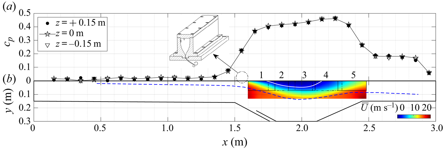
Figure 1. (a) Average wall-pressure coefficient  $c_p$ measured on the test-section centreline (
 $z=0\ \textrm {m}$) and at two symmetric spanwise positions (
 $z={\pm }0.15\ \textrm {m}$). (b) Profile sketch of the test section with contour plot of the longitudinal velocity (the numbers 1 to 5 refer to the particle image velocimetry measurement stations). Solid white and dashed blue lines denote the dividing streamline and the
  $\delta _{99}$ boundary-layer thickness, respectively. Inset: settling chamber and contraction of the PJA system (§ 2.2).
The position of reattachment on the test surface is strongly influenced by the presence of an FPG. This so-called suction-and-blowing configuration was specifically chosen to generate a TSB that mimics the region of separated flow in turbulent SBLIs, where the shear layer in the aft part of incident-shock or compression-ramp interactions is usually deflected towards the wall (Babinsky & Harvey Reference Babinsky and Harvey2011; Threadgill & Bruce Reference Threadgill and Bruce2020). Thus, the flow development in the current configuration is different than in flows that use a suction-only boundary condition to separate the boundary layer, and where reattachment occurs because of turbulent diffusion only (Wu et al. Reference Wu, Meneveau and Mittal2020). LeFloc'h et al. (Reference LeFloc'h, Weiss, Mohammed-Taifour and Dufresne2020) discuss the pressure distribution generated in the TFT boundary-layer wind tunnel in relation to other references from the literature.
2.2. Pulsed-jet actuators
The flow is controlled with a series of PJAs that can be placed at two streamwise positions on the test surface and that are distributed across the complete test-section span. Those actuators produce rectangular jets of velocity  $U_j(t)$ ejecting from the test-section wall at a specific frequency. They were chosen because of their relatively large control authority compared to other types of actuators, the possibility of independently controlling their forcing amplitude, frequency and duty cycle as well as their proven success in the active control of two-dimensional flow separation (Petz & Nitsche Reference Petz and Nitsche2007; Cattafesta & Sheplak Reference Cattafesta and Sheplak2011). The pulsed jets are generated using a supply line of compressed air with a pressure
  $P_j$ that imposes a given mass-flow rate. The total mass flow is controlled by eight solenoid valves which simultaneously feed a settling chamber that is mounted on top of the test surface (see inset in figure 1). The settling chamber is filled with light foam to homogenize the air flow and ensure a constant forcing amplitude across the test-section span. The flow from the settling chamber is then accelerated through a third-order polynomial shaped contraction with an area ratio of
  $50$ before reaching a series of equally spaced slots perforated on the test surface. Each slot has a width of
  $h=1\ \textrm {mm}$ in the main streamwise direction of the flow and a length of
  $6h$ in the spanwise direction. The slots are spaced
  $2\ \textrm {mm}$ apart and are built with a slant angle in the test surface so that the jets exit at
  $45^\circ$ from the horizontal direction (an image of the system is shown in Mohammed-Taifour et al. Reference Mohammed-Taifour, Le Floc'h and Weiss2020). The control signal of the solenoid valves is a square wave of frequency
  $F_j$ that can be varied between
  $0$ and
  $300\ \textrm {Hz}$. The duty cycle was fixed at
  $25\,\%$ for the duration of the experiments. The amplitude of the pulsations is controlled by an analogue pressure reducer through which the pressure-supply level
  $P_j$ can be manually controlled between 1 and 7 bar. The jet velocity
  $U_j$ corresponding to each
  $P_j$ was measured experimentally with a single hot-wire probe positioned
  $1\ \textrm {mm}$ below the test surface at the centre of slot closest to the test-section centreline. An example of time traces of
  $U_j(t)$, measured when the wind tunnel was turned on at
  $U_{ref}=25\ \textrm {m}\,\textrm {s}^{-1}$, is shown in figure 2 for a frequency of 100 Hz and four amplitudes ranging from 1 to 6 bar. Repeatability studies demonstrated that the jet velocity can be reproduced within
  $0.5\ \textrm {m}\,\textrm {s}^{-1}$ by manually controlling the supply pressure
  $P_j$. Further measurements across the span of the wind tunnel demonstrated the homogeneity of the jets outflow within a few per cent. No evidence of negative velocity (i.e. air ingestion) was observed, either when the actuators pulsed air in the main wind-tunnel flow or in a quiescent environment.
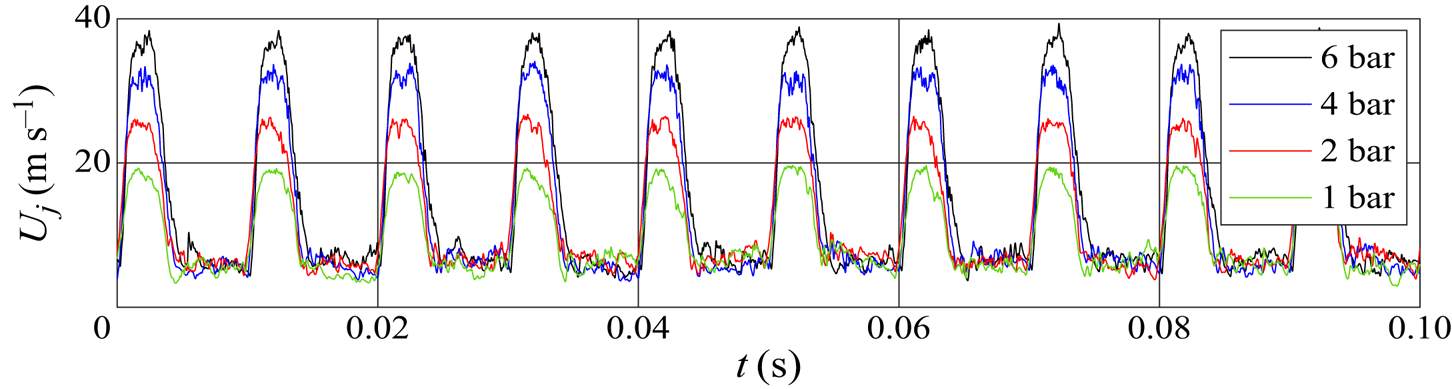
Figure 2. Exemplary time traces of the jet velocity for  $F_j = 100\ \textrm {Hz}$.
The pulsed jets are characterized by their maximum velocity  $U_{j, max}$ when the solenoid valves are open, from which we define the velocity ratio
  $\lambda _j=U_{j,max}/U_{ref}$. The momentum coefficient is defined as
  $C_\mu =(U_{j, eff} / U_{ref})^2 (h / \delta )$, where
  $U_{j, eff}$ is the effective jet velocity
  $U_{j, eff}=\sqrt {\bar {U}_j^2+(U_{j, std})^2}$,
  $h=1\ \textrm {mm}$ is the width of the control slots and
  $\delta =33\ \textrm {mm}$ is the boundary-layer thickness at
  $x=1.30\ \textrm {m}$. In the definition of the jet effective velocity,
  $\bar {U}_j$ and
  $U_{j, std}$ are the mean value and the standard deviation of the jet velocity signal
  $U_j(t)$ during a full period, respectively. Defined as such,
  $C_\mu$ represents the average momentum input of the forcing system normalized by a reference momentum in a fully incompressible flow (Greenblatt & Wygnanski Reference Greenblatt and Wygnanski2000). We further define a mass-flow coefficient
  $C_m=\dot {m}_j/ \dot {m}_{ref} = (\bar {U}_j / U_{ref})(h/h_{ts})$, where
  $h_{ts}=0.15\ \textrm {m}$ is the height of the test section at
  $x=0$ and where
  $\dot {m}_j$ and
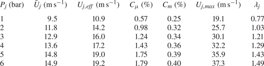
  $\dot {m}_{ref}$ are the mass-flow rates of the jet and the main stream in the wind tunnel, respectively. Table 1 recaps the values of
  $\lambda _j$,
  $C_\mu$, and
  $C_m$ as a function of the supply pressure
  $P_j$ for frequency
  $F_j=100\ \textrm {Hz}$ (figure 2). Note that, at a fixed value of the supply pressure
  $P_j$,
  $\lambda _j$,
  $C_\mu$ and
  $C_m$ vary slightly as a function of
  $F_j$.
Table 1. PJA parameters for  $F_j=100\ \textrm {Hz}$.
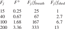
The non-dimensional forcing frequency  $F^+=F_j L_b/U_{ref}$, where
  $L_b=0.42\ \textrm {m}$ is the average length of the unforced backflow region on the test-section centreline, is provided in table 2, together with the ratios of several forcing frequencies used in the experiments to the characteristic frequencies of the breathing and shedding modes of the unforced flow (see § 3).
Table 2. Non-dimensional forcing frequency  $F^+=F_j L_b/U_{ref}$ and ratio of several forcing frequencies to the characteristic frequencies of the breathing and shedding modes of the unforced flow:
  $f_{breath} \simeq 0.6\ \textrm {Hz}$ and
  $f_{shed} \simeq 15\ \textrm {Hz}$, respectively.
2.3. Instrumentation
The experimental techniques used in the present work were essentially the same as in Mohammed-Taifour & Weiss (Reference Mohammed-Taifour and Weiss2016) and LeFloc'h et al. (Reference LeFloc'h, Weiss, Mohammed-Taifour and Dufresne2020) and will only be described briefly. The average wall pressure was measured using two Scanivalve DSA3217 pressure scanners and the wall-pressure fluctuations with several Meggitt 8507C-1 piezoresistive pressure transducers. The estimated uncertainty of the measured values is  ${\pm }0.7\,\%$ and
  ${\pm }5\,\%$ for the mean and fluctuating pressure, respectively (Weiss et al. Reference Weiss, Mohammed-Taifour and Schwaab2015). The forward-flow fraction
  $\gamma$, defined as the percentage of time that the near-wall flow goes in the main, positive streamwise direction, was measured with the microelectromechanical system (MEMS) calorimetric shear-stress sensor introduced by Weiss et al. (Reference Weiss, Schwaab, Boucetta, Giani, Guigue, Combette and Charlot2017). This sensor features three parallel micro-beams suspended over a small cavity. The middle beam is heated by an electric current and the two lateral beams act as resistance thermometers. By measuring the electrical resistance of the two lateral beams, the asymmetry of the thermal wake of the heater can be related to the wall shear stress after a dedicated calibration. In the present work, the sensor was used uncalibrated to detect the instantaneous direction of the near-wall flow in a manner similar to a classical thermal tuft (Eaton et al. Reference Eaton, Jeans, Ashjaee and Johnston1979; Schwaab & Weiss Reference Schwaab and Weiss2015). The uncertainty in
  $\gamma$ is estimated at
  ${\pm }2\,\%$ for a 180 s long signal (LeFloc'h et al. Reference LeFloc'h, Mohammed-Taifour, Dufresne and Weiss2018). All single-point unsteady signals were digitized with a 24-bit National Instruments NI-PXIe-4492 data acquisition card at a sampling rate of 2 kHz and low-passed filtered with the embedded anti-aliasing filter. Power-spectral densities were computed using Welch's modified periodogram algorithm with 50 % overlap and a Hamming window (Bendat & Piersol Reference Bendat and Piersol2010).
Planar flow velocity measurements were achieved using a high-speed, planar, two-component (2D-2C), particle image velocimetry (PIV) system that consists of a Litron LDY304 Nd:YLF laser, light-sheet optics and two Phantom V9.1 CMOS cameras mounted side by side. Both cameras were equipped with a 50 mm,  $f^{\#}2$ Micro Nikkor lens to obtain a total field of view of approximately 0.20 m in the streamwise direction and 0.075 m in the wall-normal direction. The pair of cameras was moved in the streamwise and vertical directions to cover the complete length and height of the separation bubble (see figure 1). The images were processed by the LaVision DaVis software (version 8.2) using a multi-pass correlation technique with 50 % overlap. The vector spacing in the object plane is 1 mm, which corresponds to approximately 3 % of the boundary-layer thickness at
  $x=1.3\ \textrm {m}$ (
 $\delta =33\ \textrm {mm}$). The sampling frequency was set at 400 Hz for the duration of the experiments, except for
  $F_j=15\ \textrm {Hz}$, where it was set at 450 Hz to facilitate phase averaging. The nominal uncertainty of the system, based on a 0.1 pixel displacement uncertainty, is
  $0.5\ \textrm {m}\,\textrm {s}^{-1}$ (Mohammed-Taifour & Weiss Reference Mohammed-Taifour and Weiss2016). The uncertainty in turbulence statistics, which depend on the total duration of the measurements, are
  ${\pm }0.2\ \textrm {m}\,\textrm {s}^{-1}$ for the mean streamwise velocity,
  ${\pm }0.3\ \textrm {m}\,\textrm {s}^{-1}$ for the mean wall-normal velocity,
  ${\pm }0.2\ \textrm {m}^2\,\textrm {s}^{-2}$ for the streamwise stresses,
  ${\pm }0.1\ \textrm {m}^2\,\textrm {s}^{-2}$ for the wall-normal stresses and
  ${\pm }0.1\ \textrm {m}^2\,\textrm {s}^{-2}$ for the shear stresses, respectively (LeFloc'h et al. Reference LeFloc'h, Weiss, Mohammed-Taifour and Dufresne2020).
2.4. Three-dimensional effects in the average flow
Because the test section of the wind tunnel is rectangular, three-dimensional effects in the average flow are unavoidable. Mohammed-Taifour & Weiss (Reference Mohammed-Taifour and Weiss2016) used oil-film visualizations to draw a consistent topological map of the skin-friction lines in the unforced TSB. They showed the strongly three-dimensional nature of the near-wall flow but argued that wall-normal measurements near the centreline can be considered as quasi-two-dimensional since the flow is symmetric and features a narrow band around the centreline where the wall streamlines are straight. Mohammed-Taifour, Dufresne & Weiss (Reference Mohammed-Taifour, Dufresne and Weiss2019) and LeFloc'h et al. (Reference LeFloc'h, Weiss, Mohammed-Taifour and Dufresne2020) further investigated the three-dimensional nature of the average (unforced) flow through Reynolds-averaged Navier–Stokes simulations and interpreted the directions of the wall streamlines by classical secondary-flow arguments in the sidewall boundary layers.
Oil-film visualizations on the test surface are shown in figure 3 for the unforced flow  $(a)$ and two forced cases: a relatively mild forcing where the actuators were placed at
  $x=1.45\ \textrm {m}$
  $(b)$ and a stronger forcing with actuators placed at
  $x=1.55\ \textrm {m}$
  $(c)$. In both cases the forcing frequency was 20 Hz and the supply pressure was set to 4 bar. It can be seen that the overall structure of the wall streamlines is not changed by the actuation, and that the flow remains symmetric, thus precluding any significant average spanwise velocity through the centreline. On the other hand, for relatively strong forcing, and despite the spanwise-homogeneous forcing amplitude, the separation line is strongly curved, which implies a vanishing band of quasi two-dimensional flow. This can be explained as follows: as will be discussed in § 4, forcing does not have a strong effect on the average pressure distribution in the test section, nor, consequently, on the potential streamlines. Therefore, the secondary flows on the sidewalls and the associated corner effects remain relatively unaffected. On the other hand, as can be observed in figure 3, forcing strongly changes the position of flow separation on the test-section centreline. This difference in behaviour between the centreline and the sidewalls leads to stronger three-dimensionality of the average wall streamlines when forcing is more effective.
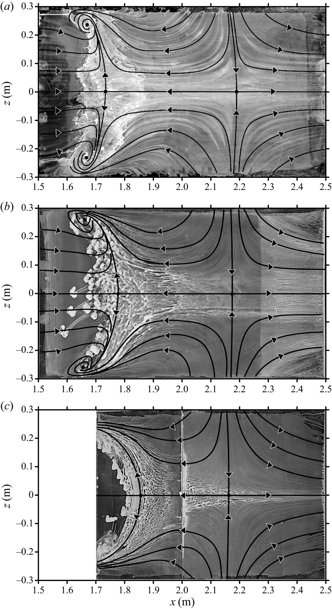
Figure 3. Sample of oil-film visualizations.  $(a)$ Unforced flow,
  $(b)$ forcing at
  $x=1.45\ \textrm {m}$ and
  $(c)$ forcing at
  $x=1.55\ \textrm {m}$ for a supply pressure of 4 bar and a forcing frequency of 20 Hz. In
  $(c)$ the upstream part of the test surface is blocked by the actuator set-up.
Despite this caveat, the measurements reported in this article were, for practical reasons, performed on the centreline of the test section. The underlying assumption is that the flow physics reported herein is locally two-dimensional, which can be substantiated by the fact that the separation line is only slightly curved between  $z=-0.1$ and
  $z=0.1\ \textrm {m}$, even when forcing is strong. Nevertheless, the consequence of this hypothesis will be further discussed in § 6.
3. The unforced flow
In this section we provide salient features of the TSB in its uncontrolled state. The presentation is limited to the material that is relevant for a discussion of the controlled cases in the next sections. Further details can be obtained in Mohammed-Taifour & Weiss (Reference Mohammed-Taifour and Weiss2016).
A contour plot of the average longitudinal velocity  $\bar {U}(x,y)$ in the unforced TSB with representative velocity vectors is shown in figure 4. As expected, the flow detaches from the wall and reattaches further downstream, thereby creating a recirculation region with negative average longitudinal velocity. The degree of detachment may be quantified by streamwise positions referring to a specific threshold of the near-wall forward-flow fraction
  $\gamma$ (Simpson Reference Simpson1989). Incipient detachment (ID) is the position where the near-wall flow is in the positive direction exactly 99 % of the time (
 $\gamma =99\,\%$) and marks the start of the separation process. At transitory detachment (TD) and transitory reattachment (TR), the flow goes in the positive and negative directions with equal probability (
 $\gamma =50\,\%$). These two positions delimit the average recirculation zone of the TSB and correspond to the usual definitions of turbulent separation and reattachment with
  $c_f=\tau _w/\frac {1}{2} \rho U^2_{ref}=0$, where
  $\tau _w$ is the average wall shear stress and
  $\rho$ is the fluid density (Coleman, Rumsey & Spalart Reference Coleman, Rumsey and Spalart2018). Finally, complete reattachment (CR) marks the very end of the separation process with
  $\gamma =99\,\%$ again. In the present case,
  $x_{ID}\simeq 1.59\ \textrm {m}$,
  $x_{TD} \simeq 1.75\ \textrm {m}$,
  $x_{TD} \simeq 2.17\ \textrm {m}$ and
  $x_{CR} \simeq 2.30\ \textrm {m}$, where
  $x=0$ marks the entrance of the test section (figure 1). Based on these values, we define two characteristic lengths of the unforced TSB:
  $L_{50}=x_{TR}-x_{TD}=0.42\ \textrm {m}$ and
  $L_{99}=x_{CR}-x_{ID}=0.71\ \textrm {m}$. For clarity, in the remainder of the article we will use
  $L_b$ to denote the length
  $L_{50}$ of the unforced flow, as in Mohammed-Taifour & Weiss (Reference Mohammed-Taifour and Weiss2016).
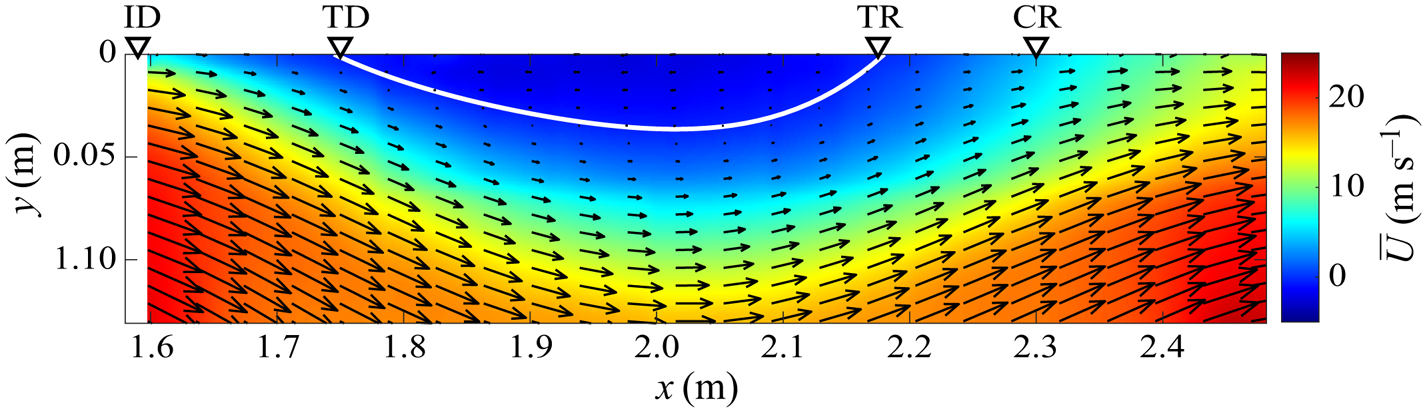
Figure 4. Averaged velocity field along the test-section centreline. The white solid line delimits  $\bar {U}=0$.
Streamwise distributions of the average wall-pressure coefficient  $c_p=(p-p_{ref})/\frac {1}{2} \rho U^2_{ref}$, the fluctuating wall-pressure coefficient
  $c_{p^{\prime }}=p_{rms} / \frac {1}{2} \rho U^2_{ref}$ and the near-wall forward-flow fraction
  $\gamma$, are shown in figure 5 (here,
  $p_{rms}$ is the root mean square of the pressure fluctuations). The slope of the
  $c_p$ distribution is very steep between
  $x=1.45\ \textrm {m}$ and
  $x = 1.65\ \textrm {m}$ and decreases afterwards when the shear layer detaches from the wall. The maximum of
  $c_p$ is reached at
  $x = 2.25\ \textrm {m}$, between TR and CR, and the wall pressure subsequently decreases because of the flow acceleration induced by the convergence of the tunnel floor. The fluctuating pressure coefficient
  $c_{p^{\prime }}$ shows a bi-modal character with a first local maximum close to ID and a second, global maximum close to CR. As demonstrated by LeFloc'h et al. (Reference LeFloc'h, Weiss, Mohammed-Taifour and Dufresne2020), the first maximum is caused by the superposition of two separate phenomena occurring at approximately the same streamwise position: first, the pressure signature of the low-frequency breathing motion of the TSB and second, the effect of the APG on the turbulent structures responsible for the pressure fluctuations in the attached boundary layer, which shifts the energy of the pressure fluctuations to lower frequencies. The second maximum of the
  $c_{p^{\prime }}$ distribution is associated with the convection of large structures within the shear layer and their subsequent shedding downstream of the TSB (Mohammed-Taifour & Weiss Reference Mohammed-Taifour and Weiss2016; LeFloc'h et al. Reference LeFloc'h, Weiss, Mohammed-Taifour and Dufresne2020).
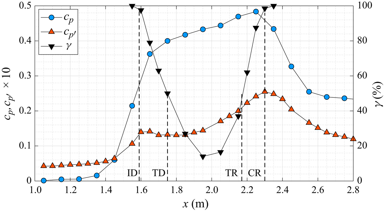
Figure 5. Averaged and fluctuating pressure coefficients and forward-flow fraction along the test-section centreline.
The spectral content of the wall-pressure signatures at  $x=1.60\ \textrm {m}$ (ID) and
  $x=2.30\ \textrm {m}$ (CR) is shown in figure 6. A medium-frequency activity is apparent as a broad peak in the p.s.d. at approximately 15–20 Hz in the reattachment region. This unsteadiness is linked to the convective roll-up and shedding of vortical structures in the separated shear layer that are responsible for the second peak of
  $c_{p^{\prime }}$ in figure 5. The structures are initiated between ID and TD and most likely grow downstream through a pairing-like process similar to that occurring in turbulent free shear layers. As they are convected downstream at a velocity of approximately
  $U_c = 0.3 U_{ref}$, the structures are then accelerated towards the wall in the FPG zone and produce a maximum wall-pressure signature at the edge of the separation bubble near CR (Weiss et al. Reference Weiss, Mohammed-Taifour and Schwaab2015; Mohammed-Taifour & Weiss Reference Mohammed-Taifour and Weiss2016). When scaled with the average length of the recirculation zone, the shedding frequency of the structures is of the order of
  $St_s=fL_b/U_{ref}=0.25\text {--}0.35$. Given the convective velocity of
  $U_c \simeq 0.3 U_{ref}$, this implies that there is on average only approximately one large structure within the streamwise length
  $L_b$ of the TSB.
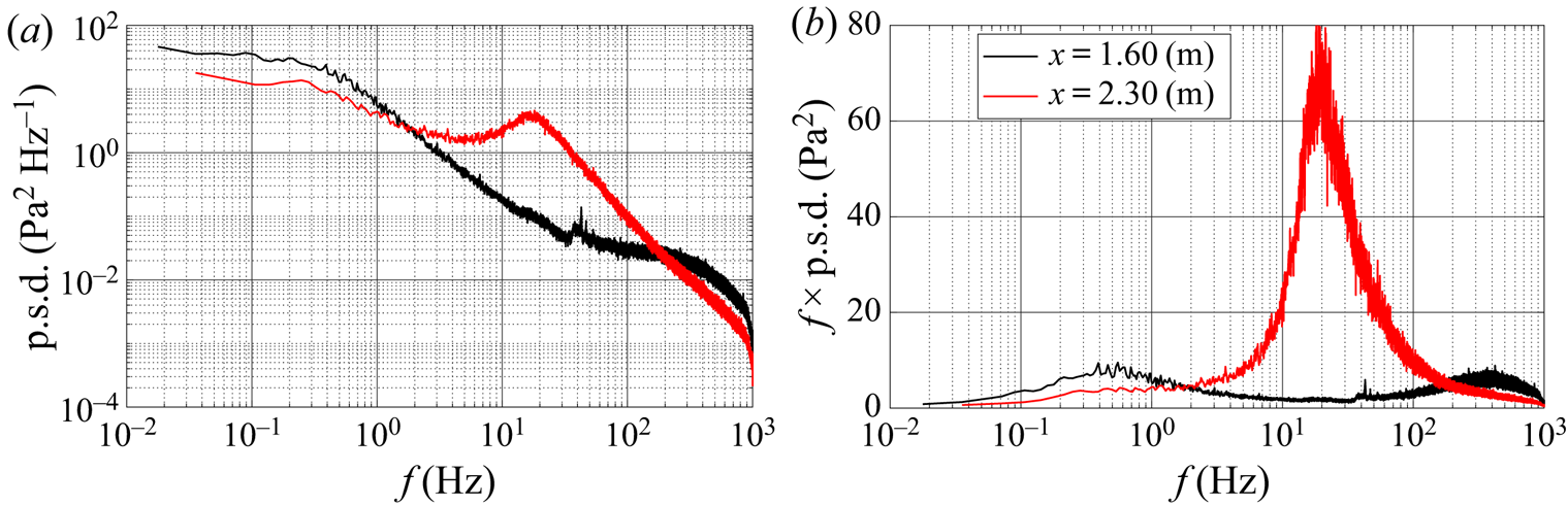
Figure 6. The p.s.d. ( $a$) and pre-multiplied p.s.d. (
 $b$) of wall-pressure fluctuations at the local and global maxima of
  $c_{p'}$.
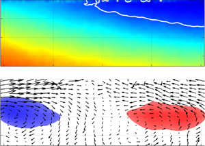
The low-frequency unsteadiness of the TSB is most apparent at  $x=1.60\ \textrm {m}$, where it emerges as a hump with a central frequency of 0.6 Hz in the pre-multiplied spectrum. This low-frequency pressure signature is also present in the reattachment zone, albeit at a lower amplitude: Weiss et al. (Reference Weiss, Mohammed-Taifour and Schwaab2015) showed that when computed in a narrow frequency range characteristic of the low-frequency unsteadiness, the filtered fluctuating wall-pressure coefficient shows two distinct peaks located at the streamwise positions of maximum APG and FPG (their figure 11). With the use of two thermal-tuft probes, and following a methodology similar to that of Eaton & Johnston (Reference Eaton and Johnston1982), Weiss et al. (Reference Weiss, Mohammed-Taifour and Schwaab2015) then showed that these pressure fluctuations are the signature of a low-frequency random cycle of contraction and expansion, dubbed breathing, of the TSB. In a subsequent experiment, Mohammed-Taifour & Weiss (Reference Mohammed-Taifour and Weiss2016) demonstrated that this breathing motion is well illustrated by the first proper orthogonal decomposition mode of the velocity field (see also LeFloc'h et al. Reference LeFloc'h, Weiss, Mohammed-Taifour and Dufresne2020). Using the same scaling as above, the breathing frequency is of the order of
  $St_b=fL_b/U_{ref} \simeq 0.01$.
Both the thermal-tuft measurements of Weiss et al. (Reference Weiss, Mohammed-Taifour and Schwaab2015) and the PIV experiments of Mohammed-Taifour & Weiss (Reference Mohammed-Taifour and Weiss2016) revealed that during the random cycles of low-frequency contraction and expansion, the instantaneous detachment moves over a distance approximately twice as large as the instantaneous reattachment. However, no attempt was made to investigate a possible time lag between the low-frequency motion in the detachment and reattachment zones. Mohammed-Taifour (Reference Mohammed-Taifour2017) subsequently performed a lead–lag analysis of the wall-pressure signal between  $x_1=1.60\ \text {m} \simeq x_{ID}$ and
  $x_2=x_{CR}=2.30\ \textrm {m}$. The results are presented in figure 7. The magnitude-squared coherence function
  $C_{p'_1p'_2}$ is significantly larger than zero in the low-frequency part of the spectrum and the phase angle shows a linear dependency with the frequency, with a slope of
  $\theta _{p'_1p'_2}/2{\rm \pi} \simeq 0.044f$. This indicates that the two signals are highly correlated and that there is an average delay of 44 ms between the pressure signal at CR compared to the signal at ID (Bendat & Piersol Reference Bendat and Piersol2010). In other words, the instantaneous (low-frequency) reattachment moves after the instantaneous detachment. The time delay of 44 ms corresponds to the time that it takes for a fluid particle to follow an average streamline between the streamwise positions of ID and CR in the potential flow outside of the boundary layer. From the average velocity field shown in figure 4, the length of such a streamline starting at (
 $x=1.60\ \textrm {m}$,
  $y=0.04\ \textrm {m}$) and integrated until
  $x=2.30\ \textrm {m}$ is 0.80 m. The average potential-flow velocity between ID and CR can be estimated from an average pressure coefficient
  $\widetilde {c_p}$ between these two positions. From figure 5 we obtain
  $\widetilde {c_p} \simeq 0.42$, which implies a potential velocity of
  $U_{pot} \simeq U_{ref} \sqrt {1-\widetilde {c_p}}=19\ \textrm {m}\,\textrm {s}^{-1}$. Dividing the length of the streamline (0.80 m) by this velocity gives an estimated convection time of 42 ms, which is indeed very close to the time delay obtained from the lead–lag analysis. This convection time is much shorter than the characteristic period of the low-frequency breathing motion, which, in this flow, is of the order of 1 s.
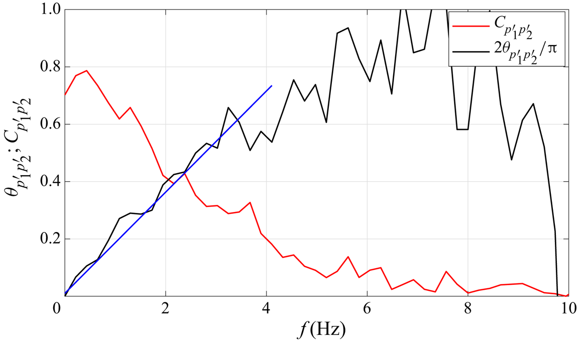
Figure 7. Magnitude-squared coherence  $C$ and phase angle
  $\theta$ of the low-frequency component of the wall-pressure fluctuations measured at
  $x_1=1.60\ \text {m} \simeq x_{ID}$ and
  $x_2=x_{CR}=2.30\ \textrm {m}$. The blue line is a linear fit on the phase angle between
  $0$ and
  $4\ \textrm {Hz}$.
Figure 8( $a$) shows distributions of the correlation coefficient between the low-pass filtered wall-pressure fluctuations measured at two reference positions (
 $x=1.65\ \textrm {m}$ and
  $x=2.30\ \textrm {m}$) and other streamwise positions on the test-section centreline. These data were obtained by low-pass filtering the pressure signal at
  $f =10\ \textrm {Hz}$ to concentrate on the low-frequency breathing motion. As mentioned above, the correlation coefficient is high between the two reference points, but turns slightly negative when the moving probe is located between TD and TR. This indicates that when the wall pressure is increasing at the upstream and downstream edges of the TSB, it decreases in the middle, and vice versa. This suggests a simple model of the low-frequency breathing where the modulation of the TSB size is associated with a slow, quasi-steady contraction and expansion of the average wall-pressure distribution is a manner sketched in figure 8(
 $b$). A contraction of the TSB induces a decrease of the wall pressure at the edges of the TSB and an increase within the recirculation zone. The variation of the wall pressure that occurs near ID during this quasi-steady motion is responsible for the low-frequency pressure signature observed in figure 6.
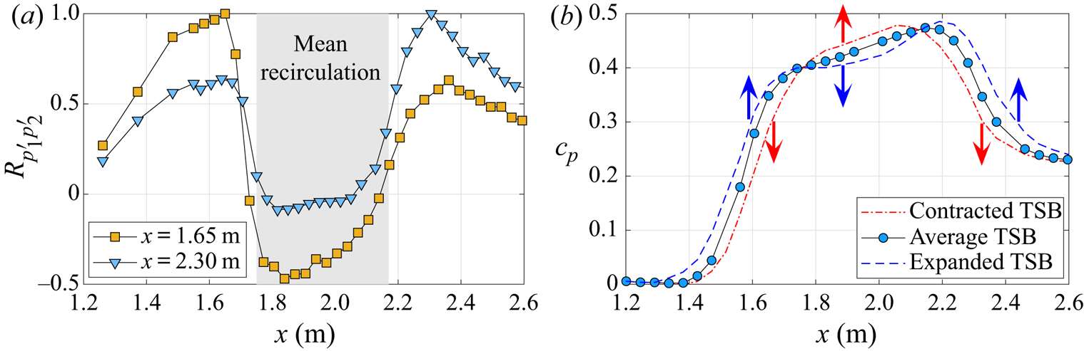
Figure 8. ( $a$) Correlation coefficient between the low-pass filtered pressure fluctuations measured at reference positions
  $x=1.65\ \textrm {m}$ and
  $x=2.30\ \textrm {m}$ and a moving point on the test-section centreline. (
 $b$) Conceptual model of the contraction and expansion of the average pressure distribution.
In summary, the unforced TSB investigated in this work naturally contracts and expands at a frequency of the order of one Hertz. This low-frequency ‘breathing’ motion is most likely driven by an upstream mechanism that acts on the separation position first. The shift of the separation front triggers a change of the overall pressure distribution and leads to a motion of the reattachment position in the direction opposite of separation. This proposed mechanism will be further discussed in § 6 in light of the results obtained with periodic forcing.
4. Continuous forcing
We begin with a presentation of the results obtained while the flow was continuously forced at a specific frequency and amplitude. The pulsed-jet actuators were installed at two streamwise positions in the test section: first at the beginning of the pressure rise ( $x=1.45\ \textrm {m}$) and second within the APG zone (
 $x=1.55\ \textrm {m}$). The resulting distributions of forward-flow fraction on the tunnel centreline, measured with the MEMS calorimetric sensor, are presented in figure 9. These data were obtained for a supply pressure
  $P_j=4\ \textrm {bar}$, which corresponds to a nominal velocity ratio of
  $\lambda _j=1.4$ and a momentum coefficient of
  $C_{\mu }=1.4\,\%$, with variations of
  ${\pm }0.1$ and
  ${\pm }0.06\,\%$ depending on the frequency, respectively. At
  $x=1.55\ \textrm {m}$, steady forcing at
  $f=0\ \textrm {Hz}$ was also tested. For this, the supply pressure was reduced manually so as to match the nominal momentum coefficient of
  $C_{\mu }=1.4\,\%$.
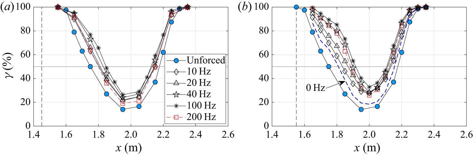
Figure 9. Forward-flow fraction  $\gamma$ for the unforced and forced flows with
  $P_j=4 \ \textrm {bar}$ (
 $C_\mu =1.4\,\% \pm 0.06\,\%)$. Forcing position at
  $x=1.45\ \textrm {m}$ (
 $a$) and at
  $x=1.55\ \textrm {m}$ (
 $b$). Vertical dashed lines indicate the streamwise position of actuation.
The distributions of  $\gamma$ show the familiar U shape indicative of an increased amount of backflow within the TSB. For all frequencies, the distributions are narrower with forcing compared to the unforced case. This shows that forcing reduces the size of the TSB by pushing the average separation point (TD) downstream and the average reattachment point (TR) upstream. Interestingly, forcing appears to move TD approximately twice as far as TR, and that irrespective of the forcing frequency. The most effective frequency which results in the smallest TSB (minimum
  $L_{50}$) is
  $F_j=100\ \textrm {Hz}$ at both streamwise positions, although the changes in
  $L_{50}$ above
  $F_j=40\ \textrm {Hz}$ are relatively small. When scaled with the average backflow length
  $L_b$ of the unforced TSB,
  $F_j=100\ \textrm {Hz}$ is equivalent to
  $F^+=F_j L_b /U_{ref}=1.7$, which is of the same order of magnitude as the most effective frequencies reported by Greenblatt & Wygnanski (Reference Greenblatt and Wygnanski2000) in typical AFC applications (see also table 2). Furthermore, the results demonstrate that periodic forcing is more effective than steady blowing (
 $f=0\ \textrm {Hz}$) in reducing the size of the TSB, which is consistent with virtually all known results on active separation control (Greenblatt & Wygnanski Reference Greenblatt and Wygnanski2000).
Representative distributions of the average wall-pressure coefficient  $c_p$ for
  $C_\mu = 1.4\,\%$ and
  $1.8\,\%$ are presented in figure 10, again for the two forcing positions. The effect of forcing on
  $c_p$ is much smaller than on
  $\gamma$ and the pressure distributions are only slightly altered. Nevertheless, the variations of
  $c_p$ are larger than the measurement uncertainty of the pressure transducers (§ 2.3) and than the spanwise variations in the unforced flow (figure 1). The trend is similar for both forcing positions, with a decrease of
  $c_p$ at the edges of the TSB and an increase between TD and TR. This behaviour is consistent with a reduction of the TSB size through forcing since a smaller TSB is associated with an increased pressure recovery in the separated region. Both the forward-flow fraction and the average pressure distributions indicate that forcing at
  $x=1.55\ \textrm {m}$ is more effective than at
  $x=1.45\ \textrm {m}$, which is most likely correlated with the larger distance between the actuators and the unforced position of TD in the latter case. Thus, in the remainder of the article we will concentrate on forcing at
  $x=1.55\ \textrm {m}$.
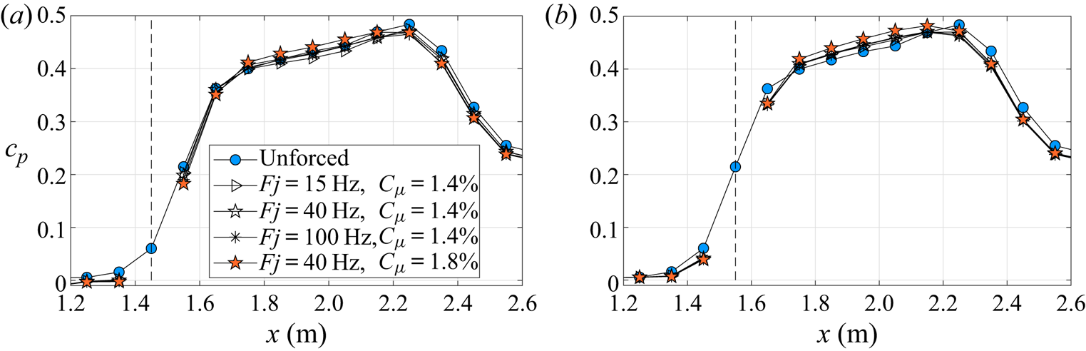
Figure 10. Average wall-pressure coefficient  $c_p$ for the unforced and forced flows at varying forcing frequencies and amplitudes. Forcing position at
  $x=1.45\ \textrm {m}$ (
 $a$) and at
  $x=1.55\ \textrm {m}$ (
 $b$). Vertical dashed lines indicate the streamwise position of actuation.
The effect of the forcing amplitude is shown in figure 11 at the most effective frequency  $F_j=100\ \textrm {Hz}$. Clearly, increasing
  $C_{\mu }$ decreases the size of the TSB with, again, more effect on separation than reattachment. At the maximum amplitude of
  $C_{\mu }=1.8\,\%$ (
 $P_j=6\ \textrm {bar}$), the average recirculation region is almost completely eliminated on the test-section centreline, with a minimum forward-flow fraction just below 50 %. It also appears that while the effect on TD and TR is relatively strong, the displacement of ID and CR is more limited. Thus, the characteristic length
  $L_{50}=x_{TR}-x_{TD}$ decreases more than
  $L_{99}=x_{CR}-x_{ID}$ when forcing is applied. These results are consistent with those obtained at other frequencies and amplitudes, which are summarized in figure 12. We conclude that the TSB length can be artificially reduced by periodic forcing in the boundary layer upstream of the average separation point. Increasing the amplitude of forcing has the strongest effect on the positions of TD and, to a lesser extent, on TR, while the positions of ID and CR are relatively unaffected. Finally, figure 12(
 $a$) clearly demonstrates that the differences in TSB length above
  $F_j=40\ \textrm {Hz}$ are minimal.
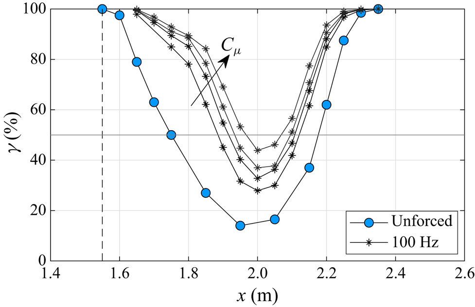
Figure 11. Forward-flow fraction  $\gamma$ for the unforced and forced flows with
  $F_j=100\ \textrm {Hz}$ and varying jet amplitudes
  $C_\mu =1.24\,\%$,
  $1.43\,\%$,
  $1.75\,\%$ and
  $1.79\,\%$. Forcing position at
  $x=1.55\ \textrm {m}$ (vertical dashed line).
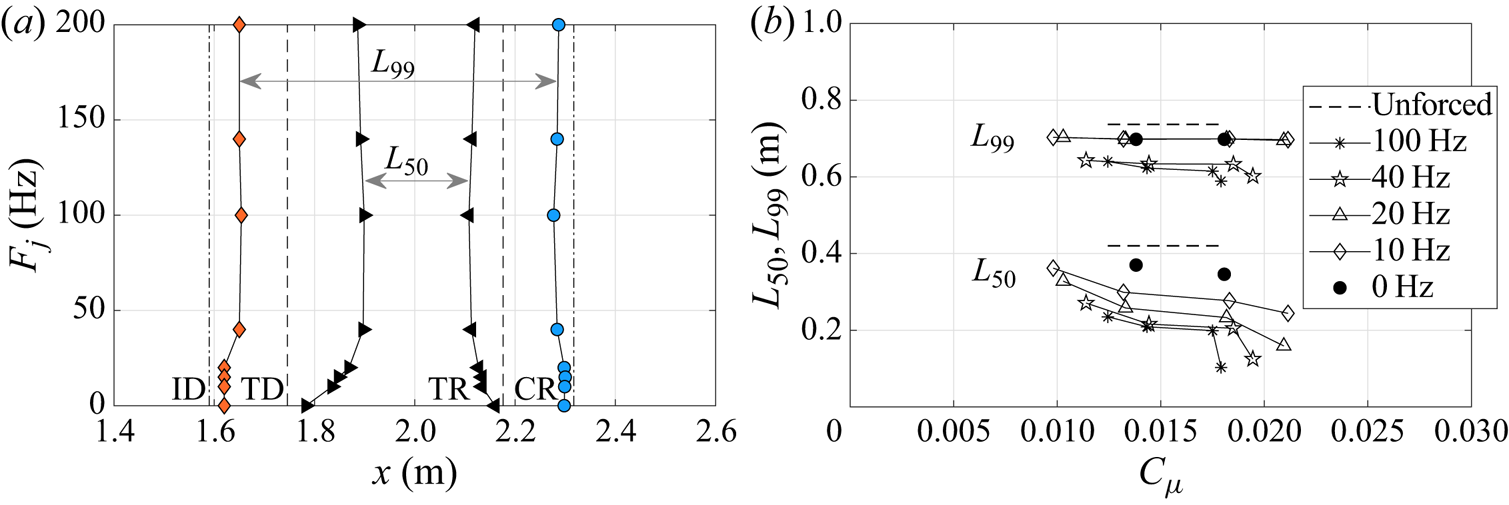
Figure 12. ( $a$) Positions of ID/CR (
 $\gamma =99\,\%$) and TD/TR (
 $\gamma =50\,\%$) for unforced (dashed lines) and forced (solid lines) flows with
  $C_\mu =1.4\,\% \pm 0.06\,\%$. (
 $b$) Characteristic lengths
  $L_{50}$ and
  $L_{99}$ as function of
  $C_\mu$ and
  $F_j$. Forcing position at
  $x=1.55\ \textrm {m}$.
Contour plots of the average vorticity and the turbulence statistics measured by PIV at  $C_{\mu } \simeq 1.4\,\%$ and varying forcing frequencies are presented in figure 13. These data were obtained by averaging over a total measuring time of 27 s, which led to the uncertainty brackets quoted in § 2.3. In all plots the white line delimits the region of mean backflow, which is shown to decrease in size with increasing frequency. At
  $F_j=100\ \textrm {Hz}$, both the length and height of the recirculation region are significantly reduced compared to the unforced case. In accordance with the MEMS calorimetric sensor data of figure 9(
 $b$), the left intersection of the
  $U=0$ isoline with the
  $x$ axis (which corresponds to the TD point), moves more than the right intersection (TR). This shows again that separation is more displaced by periodic forcing than reattachment.
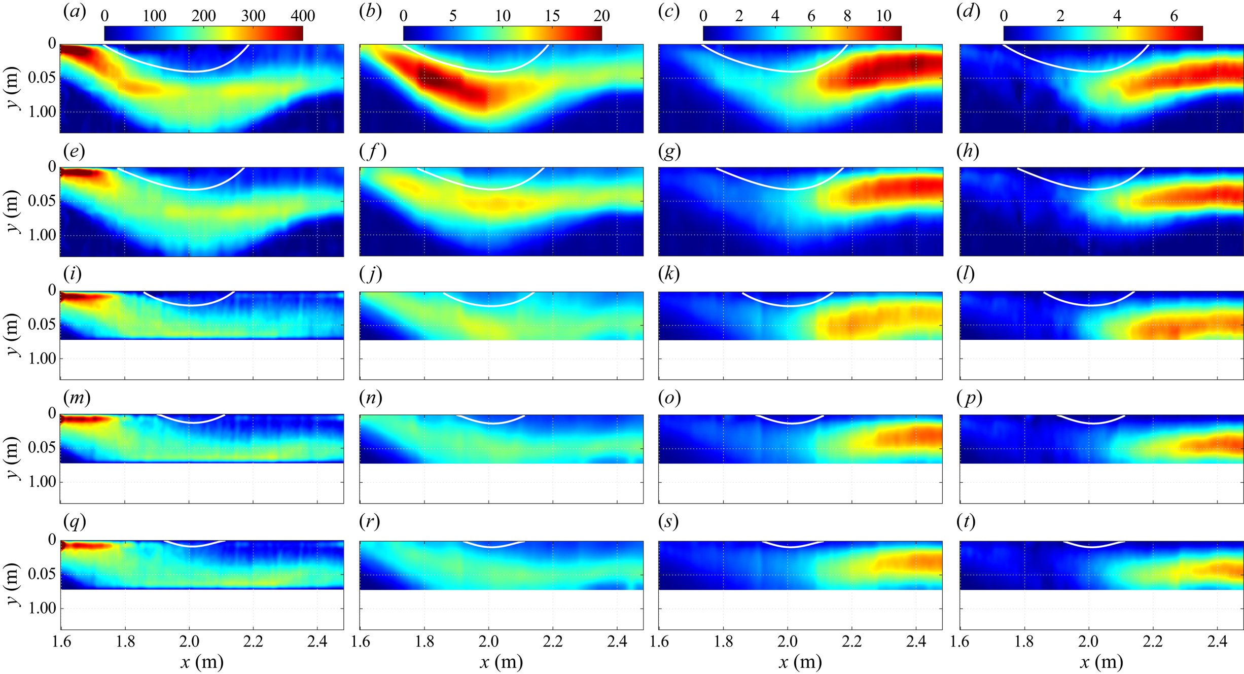
Figure 13. Contour plots of  $-\overline {\omega _z}$ in s
 $^{-1}$,
  $\overline {u'u'}/U_{ref}^2$,
  $\overline {v'v'}/U_{ref}^2$ and
  $-\overline {u'v'}/U_{ref}^2$ (from (a,e,i,m,q) to (d,h,l,p,t), respectively). Unforced (a,b,c,d) and forced flow with
  $C_\mu =1.4\,\% \pm 0.06\,\%$ and
  $F_j=0$,
  $15$,
$15$,  $40$ and
  $100\ \textrm {Hz}$ (from (e,f,g,h) to (q,r,s,t), respectively). Reynolds stresses are multiplied by
  $10^3$. The white line depicts the iso-line
  $U=0$. Forcing position at
  $x=1.55\ \textrm {m}$.
Crucially, the amplitude of all turbulence statistics appears to decrease while the TSB size is reduced by increasing the forcing frequency. This is contrary to most existing results on periodic forcing in flows where the separation point is fixed by a geometric singularity or constrained by a sufficiently strong curvature, and where earlier reattachment is achieved by enhancing the turbulent kinetic energy in the shear layer. In such flows the most effective frequency is close to the unforced shedding frequency of the separated shear layer (Chun & Sung Reference Chun and Sung1996; Kiya et al. Reference Kiya, Shimizu and Mochizuki1997; Brunn & Nitsche Reference Brunn and Nitsche2003). Excitation near the shedding frequency enhances vortex merging and turbulent fluctuations in the shear layer. This increases entrainment and intensifies the momentum transfer with the outer flow, thus resulting in earlier reattachment (Bhattacherjee et al. Reference Bhattacherjee, Troutt and Scheelke1986; Brunn & Nitsche Reference Brunn and Nitsche2006; Dandois et al. Reference Dandois, Garnier and Sagaut2007). In contrast, the effect of forcing appears to be different in the present pressure-induced TSB where the separation point is free to move on the test surface. Here, periodic forcing pushes separation downstream and reattachment upstream, while the most effective frequency is a multiple of the natural shedding frequency. This creates a smaller TSB and, consequently, reduces the turbulent fluctuations in the shear layer in a manner similar to what is observed in pressure-induced TSBs of different sizes (LeFloc'h et al. Reference LeFloc'h, Weiss, Mohammed-Taifour and Dufresne2020). The streamwise stresses appear to be reduced the most, with a decrease of approximately  $50\,\%$ between the unforced case and
  $F_j=100\ \textrm {Hz}$. Instead of showing a strong peak in the upstream half of the unforced TSB, the streamwise variation of
  $\rho \overline {u'u'}$ is essentially flat when forcing is applied, even at
  $F_j=0\ \textrm {Hz}$. The wall-normal and shear stresses
  $\rho \overline {v'v'}$ and
  $-\rho \overline {u'v'}$ decrease only by approximately
  $20\,\%$ and keep their maxima at the same streamwise position in the downstream part of the TSB. This shows again that the shear layer is strongly affected near detachment but less so near reattachment. In fact, although the size of the average backflow region is strongly diminished with forcing, the downstream part of the shear layer appears to behave in a similar way with or without forcing.
The contour plots of average vorticity (figure 13a,e,i,m,q) confirm these findings by showing that periodic forcing redistributes vorticity close to the test surface in the detachment region. The separating shear layer, which is characterized by a region of increased (negative) vorticity in the wall-normal direction upstream of TD, is wider when forcing is applied because the distance between ID and TD increases (see figure also 12 $a$). This spreading decreases the average shear and consequently reduces the streamwise stresses. In contrast, the vertical extent of the shear layer remains relatively constant in the downstream half of the TSB (
 $x>2\ \textrm {m}$), which limits the decrease in wall-normal and shear stresses. Furthermore, results from a triple decomposition of the velocity fields (not shown here), where the contribution of the coherent components at the forcing frequency and its harmonics are removed from the turbulent quantities (Hussain & Reynolds Reference Hussain and Reynolds1970), did not show any significant difference with the Reynolds decomposition of figure 13. This is a further indication that forcing with PJAs does not have a strong effect on the development of the shear layer but mostly affects the position of separation.
The p.s.d.s of wall-pressure fluctuations measured at  $x=2.35\ \textrm {m}$ (near CR) are shown in figure 14. The shape of the p.s.d.s is not affected by forcing and the ‘natural’ shedding signature at 15–20 Hz can be observed irrespective of the forcing frequency. The narrow peak at the forcing frequency for
  $F_j=15\ \textrm {Hz}$ shows that large-scale vortices are slightly more coherent in this case but there does not appear to be a strong lock-on effect when forcing is applied close to the shedding frequency, as seen for example by Bhattacherjee et al. (Reference Bhattacherjee, Troutt and Scheelke1986) behind a backward-facing step or by Kotapati et al. (Reference Kotapati, Mittal, Marxen, Ham, You and Cattafesta2010) in a laminar separation bubble. For frequencies above 5 Hz, the amplitude of the forced p.s.d.s is moderately reduced compared to the unforced case, in accordance with the reduction in turbulent stresses. This confirms that forcing only slightly affects the dynamics of the shear layer wrapping the backflow region.
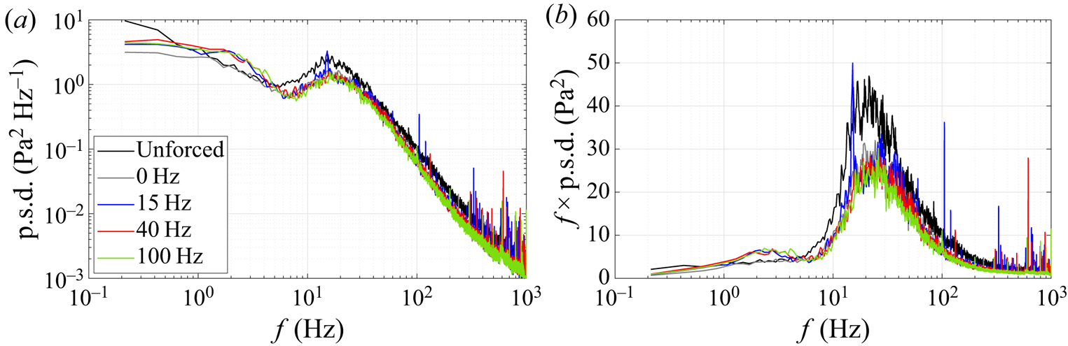
Figure 14. The p.s.d.s of wall-pressure fluctuations for the natural and forced flows,  $x=2.35\ \textrm {m}$:
  $(a)$ standard representation and
  $(b)$ pre-multiplied representation.
Phase-averaged velocity fields obtained by PIV were analysed in an attempt to better understand the mechanism sustaining the reduction in TSB size. Figure 15 shows that periodic forcing generates a vortex system that is convected in the downstream direction close to the test surface. This vortex system is made visible by contours of the  $\varGamma _2$ criterion introduced by Graftieaux, Michard & Grosjean (Reference Graftieaux, Michard and Grosjean2001) and computed here after subtracting the mean velocity
  $\bar {U}(x,y)$ from the phase-averaged fields. In addition, the position of the vortices and their direction of rotation is highlighted by a dashed line that was manually placed based on the observation of the local velocity vectors. For
  $F_j<200\ \textrm {Hz}$ the signature of the vortex system in the two-dimensional PIV plane is a pair of contra-rotating vortices aligned in the streamwise direction, with a positive vortex (clockwise) upstream of a negative one. The combination of positive and negative vorticity generates a channel of positive vertical velocity that moves fluid away from the test surface at each forcing cycle. This is reminiscent of the ‘moving pump’ concept of Darabi & Wygnanski (Reference Darabi and Wygnanski2004a), although in their case the forcing through a loudspeaker acted on the shear layer by promoting the formation of a series of negative-vorticity structures. The present mechanism is different inasmuch as the contra-rotating vortices appear as the key elements that remove low-momentum fluid away from the wall.
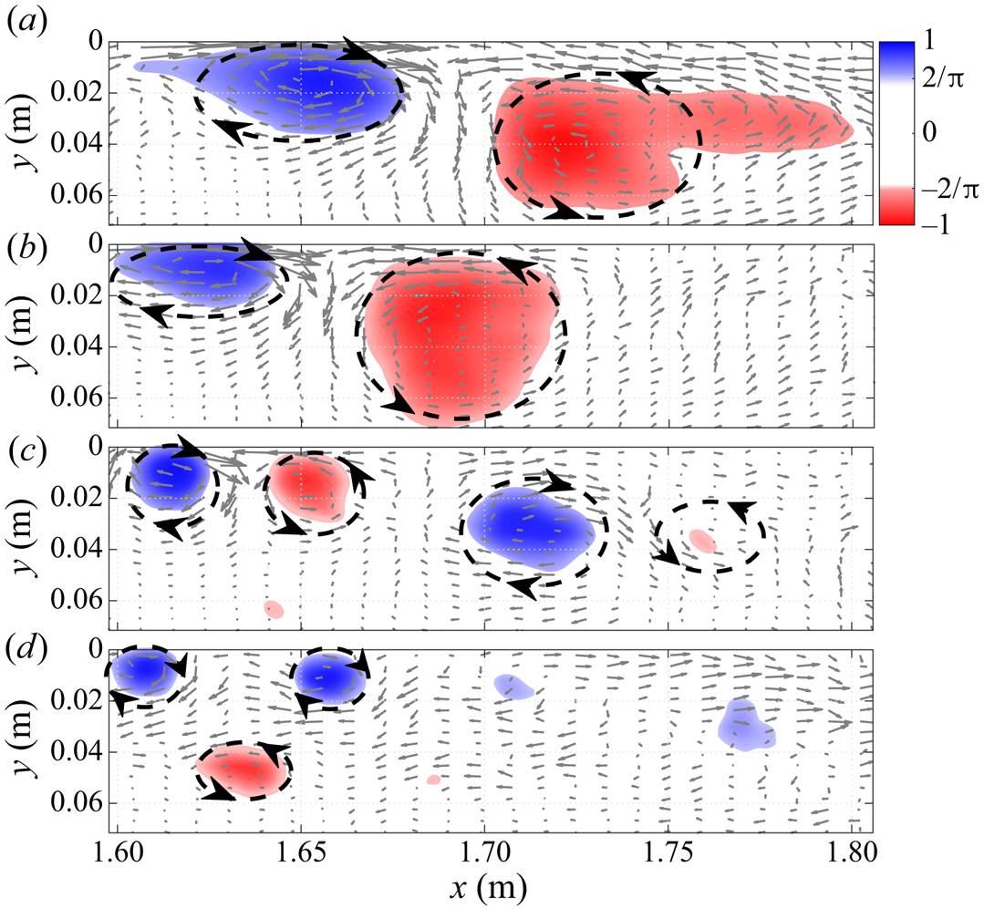
Figure 15. Illustration of vortical flow dynamics in the first PIV station with contour maps of  $\varGamma _2 \leq -2/{\rm \pi}$ (counter-clockwise) and
  $\varGamma _2 \geq 2/{\rm \pi}$ (clockwise). Panels (a) to (d) show
  $F_j=15\ \textrm {Hz}$,
  $F_j=40\ \textrm {Hz}$,
  $F_j=100\ \textrm {Hz}$ and
  $F_j=200\ \textrm {Hz}$, respectively, with
  $C_\mu =1.4\,\%$ for all frequencies;
  $\varGamma _2$ was computed after subtracting the mean velocity field from the phase-averaged field.
A similar mechanism has already been described by Hecklau et al. (Reference Hecklau, Salazar and Nitsche2013), who investigated the active control of flow separation in a one-sided diffusor. They interpreted the contra-rotating vortices observed in the PIV plane as the two-dimensional signature of the three-dimensional starting vortex generated by a PJA slot. The starting vortex is created by the rapid ejection of fluid through the inclined slot in the test surface and its size depends, among other parameters, on the amount of ejected fluid (Steinfurth & Weiss Reference Steinfurth and Weiss2020). Because the duty cycle was kept constant in the present experiment, a higher forcing frequency results in a smaller amount of fluid ejected through the slots and, consequently, a smaller vortex diameter. While there is only one pair of relatively large vortices visible in the two-dimensional measurement station for  $F_j=15\ \textrm {Hz}$ and
  $F_j=40\ \textrm {Hz}$, there are two pairs at
  $F_j=100\ \textrm {Hz}$ and, presumably, four at
  $F_j=200\ \textrm {Hz}$. At the latter frequency, the vortex system does not appear so clearly anymore because of the small amount of fluid ejected and the short time period between the pulses. It is also apparent that the high-frequency vortices tend to dissipate faster in the streamwise direction than the lower frequency, larger structures. This reduces the amount of fluid that is pumped away from the wall and may explain why forcing at
  $F_j=200\ \textrm {Hz}$ is less effective than at
  $F_j=100\ \textrm {Hz}$.
The effect of the vortex system on the separation front is illustrated in figures 16 and 17 for  $F_j=15\ \textrm {Hz}$ and
  $F_j=100\ \textrm {Hz}$, respectively. Each figure illustrates one full cycle of forcing by showing snapshots extracted from supplementary movies 1 and 2 available at https://doi.org/10.1017/jfm.2021.77. In both figures the white line delimits the region of phase-averaged backflow. Here also, the position of the vortices and their direction of rotation is highlighted by dashed lines based on the direction of the phase-averaged velocity vectors.
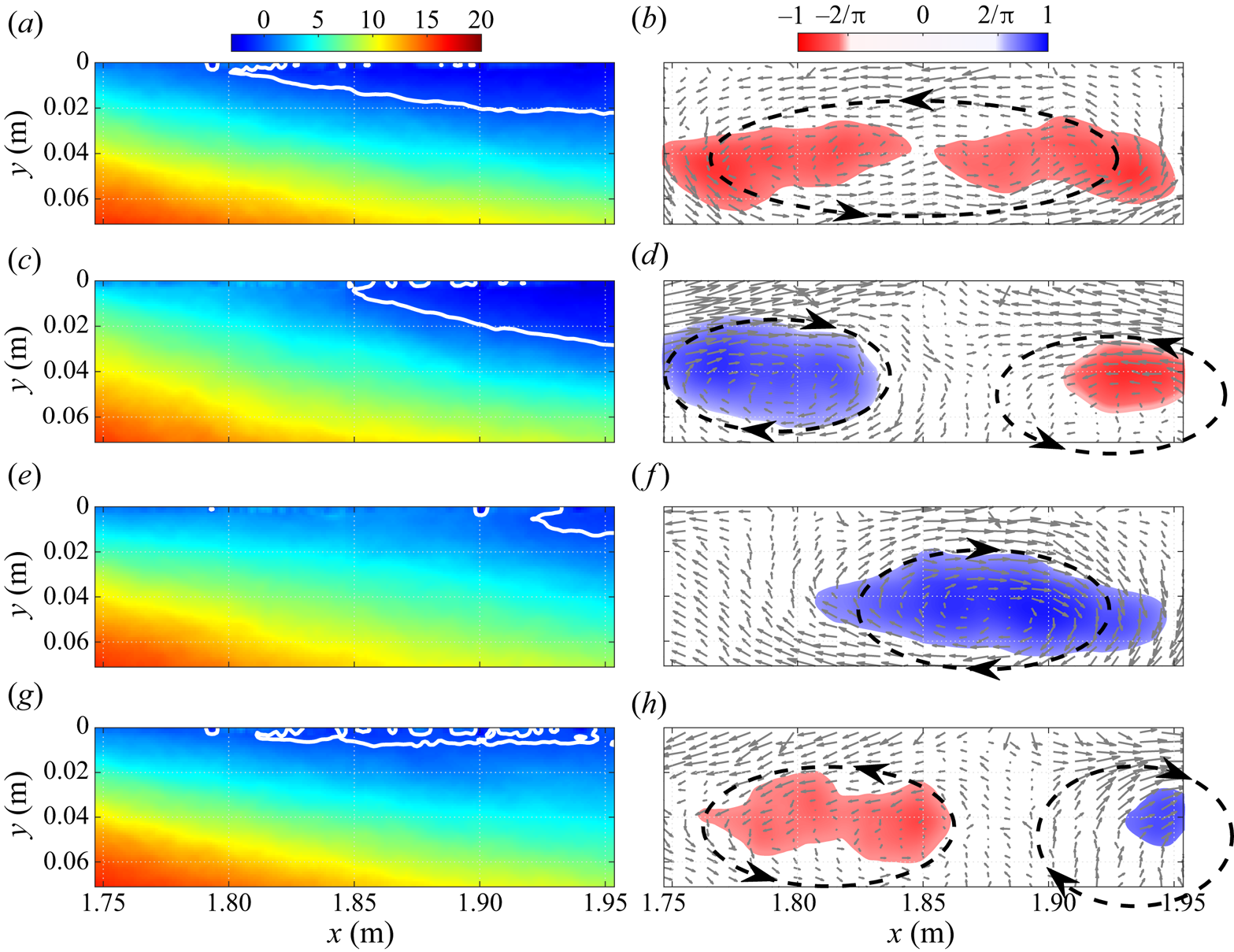
Figure 16. Illustration of the flow dynamics for  $F_j=15\ \textrm {Hz}$ and
  $C_\mu =1.4\,\%$ in PIV station 2 with contours of phase-averaged streamwise velocity (a,c,e,g) and
  $\varGamma _2$ (b,d,f,h). Time delay of 15.3 ms (approximately one quarter of a period) between the snapshots from (a,b) to (g,h). See also supplementary movie 1.
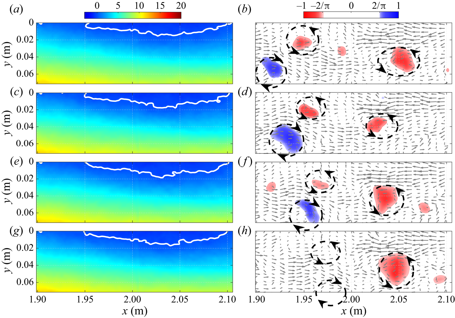
Figure 17. Illustration of the flow dynamics for  $F_j=100\ \textrm {Hz}$ and
  $C_\mu =1.4\,\%$ in PIV station 3 with contours of phase-averaged streamwise velocity (a,c,e,g) and
  $\varGamma _2$ (b,d,f,h). Time delay of 2.5 ms (one quarter of a period) between the snapshots from (a,b) to (g,h). See also supplementary movie 2.
At  $F_j=15\ \textrm {Hz}$ (figure 16) the sequence starts with a relatively large region of instantaneous backflow and a counter-clockwise vortex spanning almost the entire field of view. At the next time step the clockwise vortex enters the field and the instantaneous separation front is pushed downstream. Between the second and third time steps both the clockwise vortex and the separation front continue their downstream sweep. This results in a much smaller region of phase-averaged backflow compared to the start of the sequence. Finally, in the last time step the counter-clockwise vortex from the next period enters the field of view and the separated zone grows back to its original size. Supplementary movie 1 clearly shows that the process is highly unsteady and that the instantaneous recirculation zone grows and recedes at the period of forcing. Similar plots obtained further downstream in the reattachment region (not shown here) demonstrate a very similar phenomenon where the instantaneous reattachment point moves back and forth at
  $15\ \textrm {Hz}$. When averaged over time, this motion results in a smaller TSB compared to the unforced case, as can be seen in figures 9 and 13.
The phase-averaged fields obtained at  $F_j=100\ \textrm {Hz}$ (figure 17) illustrate a strikingly different situation. At this frequency, one period of forcing corresponds to the translation of two pairs of relatively small contra-rotating vortices within the field of view. The first (upstream) pair of vortices is visible on the contours of
  $\varGamma _2$ for the first three snapshots only. In the last snapshot, the threshold of
  $\left \lvert \varGamma _2\right \rvert >2/{\rm \pi}$ is not attained but a careful inspection of the velocity vectors reveals the likely presence of the two contra-rotating vortices at their expected positions. As for the second (downsteam) structure, only its counter-clockwise half is observed, presumably because the second half of the pair has shifted out of the field of view. Furthermore, this vortex appears to move slower than its upstream counterpart because the local velocity is smaller. Nevertheless, the mechanism controlling the separation front appears to be similar to the 15 Hz case, i.e. the passage of a vortex structure is associated with a downstream shift of the separation region. In the 100 Hz case, however, the persistent arrival of new vortices essentially maintains the phase-averaged separation front at one constant streamwise position. As can be observed in supplementary movie 2, this results in an almost steady recirculation region in a phase-averaged sense. The results obtained at
  $F_j=40\ \textrm {Hz}$ (not shown here) are essentially similar to the 100 Hz case inasmuch as only a very small back-and-forth motion of the separation front at 40 Hz can be detected. We conclude that periodic forcing is more effective when the forcing frequency is significantly higher than an inherent characteristic frequency of the separation front. When this occurs, the front does not have time to move back towards its original position between two incoming structures and the TSB appears steady when phase averaged. The similarity of the results obtained at
  $F_j=40\ \textrm {Hz}$ and
  $F_j=100\ \textrm {Hz}$ compared to the
  $F_j=15\ \textrm {Hz}$ case indicates that such a situation already occurs at
  $F_j=40\ \textrm {Hz}$, which explains why there is only a limited effect of forcing above the latter frequency. Interestingly, these results bear some resemblance with those of Amitay & Glezer (Reference Amitay and Glezer2002), who used synthetic jets to control the flow separation near the leading edge of an airfoil at both low and high forcing frequencies. Forcing at
  $F^+=O(1)$ generated strong vortices that led to unsteady reattachment while forcing at
  $F^+=O(10)$ led to an essentially steady reattachment process.
In summary, the results presented in this section indicate that the size of the average TSB can be artificially reduced by periodic forcing in the upstream boundary layer. In contrast to flow cases where the separation point is fixed by the surface geometry, forcing with PJAs pushes the mean separation (strictly speaking the TD point) downstream while the mean reattachment (TR) moves upstream, thus leading to a smaller TSB and a reduction of turbulent stresses in the shear layer. Increasing the forcing amplitude decreases the size of the average TSB while the most effective range of frequencies, which leads to the smallest TSB, is of the order of 40–100 Hz Nevertheless, one may note that the use of other types of actuators may have led to a different response of the shear layer. The present results also suggest the existence of a characteristic time scale during which the TSB tries to return to its original state between two forcing inputs. Forcing at frequencies significantly higher than the inverse of this time scale (i.e. 40–100 Hz) is more effective in reducing the size of the TSB than forcing at lower frequencies. Furthermore, the phased-averaged fields offer an interesting insight into the physics of flow separation control with PJAs. In accordance with the mechanism suggested by Hecklau et al. (Reference Hecklau, Salazar and Nitsche2013), our results indicate that PJAs generate strong starting vortices that, when convected within an APG, are associated with a downstream shift of the separation front.
5. Transient forcing
The results presented above suggest that the separation front responds to upstream disturbances with a characteristic time scale. To investigate this aspect in more detail, the transient response of the TSB subjected to an abrupt starting (Off/On) or stopping (On/Off) of the periodic forcing is explored in this section.
The MEMS calorimetric sensor was used to measure the temporal evolution of the forward-flow fraction  $\gamma (t)$ when forcing was started or stopped. The procedure is illustrated in figure 18 for a stopping sequence at a forcing frequency
  $F_j=100\ \textrm {Hz}$. The forcing signal (
 $a$) is modulated with a low-frequency square-wave function at 0.5 Hz. In the first half of the square-wave period (
 $t<1\ \textrm {s}$), the forcing signal at
  $F_j=100\ \textrm {Hz}$ is on but stops abruptly at
  $t=1\ \textrm {s}$. The output of the calorimetric sensor (
 $b$) indicates that the near-wall flow direction is mostly positive for
  $t<1\ \textrm {s}$ but oscillates more strongly between positive and negative values when the forcing is stopped (
 $t>1\ \textrm {s}$). This indicates a shift of the separation front on the test surface when forcing is turned off. By ensemble averaging this signal over a large number of square-wave periods, the forward-flow fraction is obtained as a function of time (
 $c$) and the variation of the TSB size when the forcing is stopped can be observed. The ensemble-averaged data are further smoothed by a moving average filter of 0.05 s in width. The same procedure is used for starting sequences (Off/On) by considering the square-wave period starting at
  $t=1\ \textrm {s}$.
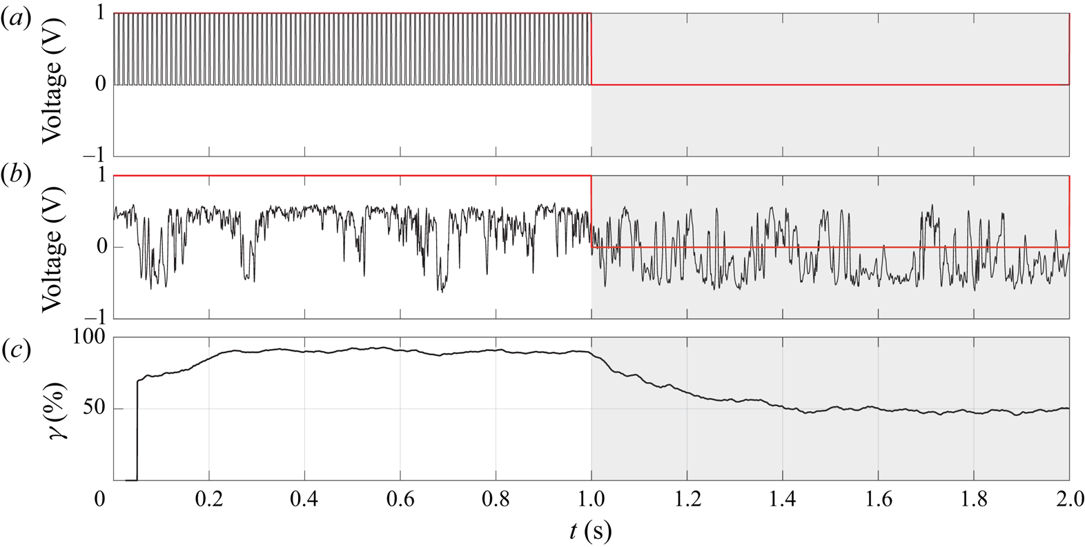
Figure 18. Illustration of the methodology used for transient forcing: ( $a$) forcing signal; (
 $b$) output of calorimetric sensor at
  $x=1.75\ \textrm {m}$; (
 $c$) forward-flow fraction computed by ensemble averaging the calorimetric sensor output over 90 square-wave periods.
The square-wave period of 2 s was chosen as a compromise that is sufficiently long to observe a complete return of the TSB to its unforced state when the forcing is started or stopped while also being sufficiently short to enable the acquisition of a large number of periods in a manageable testing time. All data reported herein were obtained by recording the calorimetric sensor signal during 180 s, which resulted in 90 square-wave periods used for ensemble averaging. The forward-flow fraction calculated at each streamwise position between  $t=0.5\ \textrm {s}$ and
  $t=1.0\ \textrm {s}$ (forcing on) and between
  $t=1.5\ \textrm {s}$ and
  $t=2.0\ \textrm {s}$ (forcing off) is compared in figure 19 to the distributions obtained in the unforced and continuously forced cases, respectively. The values of
  $\gamma$ measured with the square-wave modulated forcing signal are very close to the reference distributions, which demonstrates the validity of the methodology.
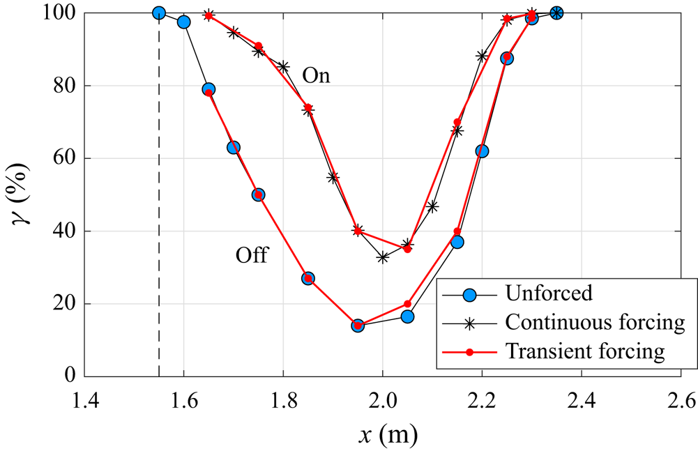
Figure 19. Comparison of forward-flow fraction distribution between unforced flow, continuous forcing, and transient forcing ( $F_j=100\ \textrm {Hz}$). Dashed line indicates position of forcing.
The transient forward-flow fraction  $\gamma (t)$ obtained with this procedure at
  $x=1.75\ \textrm {m}$ (unforced TD position) is shown in figure 20 for forcing frequencies of 15 Hz (
 $a$), 40 Hz (
 $b$) and 100 Hz (
 $c$), respectively. For
  $F_j=15\ \textrm {Hz}$, the back-and-forth motion of the separation front, already observed in figure 16, is obvious when forcing is turned on since
  $\gamma (t)$ shows an oscillatory behaviour at 15 Hz. For higher forcing frequencies, these oscillations are not observed and
  $\gamma (t)$ reaches a constant value consistent with continuous forcing after approximately 300 ms. For all forcing frequencies, the curves of
  $\gamma (t)$ show an exponential increase or decrease after
  $t = 1\ \textrm {s}$ that is reminiscent of the step response of a first-order linear system. To determine the corresponding time constants,
  $\gamma (t)$ was least-squares fitted to the following simple laws for
  $t>1\ \textrm {s}$:
 \begin{equation} \left. \begin{gathered} \gamma_{Off\text{--}On}(t) = \gamma_{Off} + (\gamma_{On} - \gamma_{Off}) \textrm{e}^{{-}t/\tau_{Off\text{--}On}}, \\ \gamma_{On\text{--}Off}(t) = \gamma_{On} + (\gamma_{Off} - \gamma_{On}) \textrm{e}^{{-}t/\tau_{On\text{--}Off}}, \end{gathered} \right\} \end{equation}
where  $\gamma _{Off}$ and
  $\gamma _{On}$ are the values of the forward-flow fraction in the unforced and continuously forced cases, respectively, and where
  $\tau _{Off\text {--}On}$ and
  $\tau _{On\text {--}Off}$ are the time constants obtained when forcing is started or stopped. The time constants are summarized in table 3, where it can be observed that
  $\tau _{Off\text {--}On}$ is almost constant for all forcing frequencies, whereas
  $\tau _{On\text {--}Off}$ is larger and increases with
  $F_j$. This indicates that the TSB takes more time to return to its unforced state when forcing is stopped than to react to a start of upstream forcing. Finally, figure 20(
 $d$) shows the transient forward-flow fraction obtained with a forcing frequency of
  $F_j=100\ \textrm {Hz}$ and forcing amplitudes varying between
  $C_{\mu }=0.57\,\%$ and
  $C_{\mu }=1.79\,\%$. In order to highlight the potential effect of the forcing amplitude on the TSB time scale, the curves of
  $\gamma (t)$ were scaled to allow their superposition on the same graph. This representation clearly shows that the values of
  $\tau _{Off\text {--}On}$ and
  $\tau _{On\text {--}Off}$, and hence the transient behaviour of the TSB, do not depend on forcing amplitude.
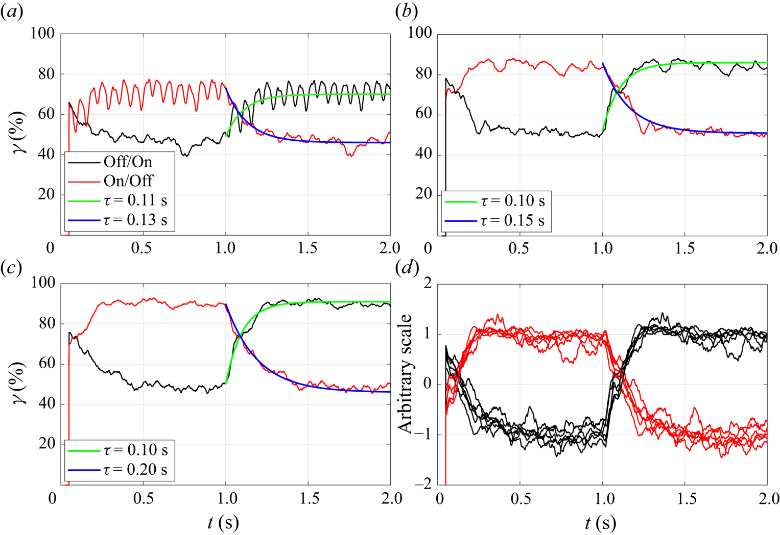
Figure 20. Transient forward-flow fraction measured at ( $a$)
$a$)  $x=1.75\ \textrm {m}$ for
  $F_j=15\ \textrm {Hz}$, (
 $b$)
$b$)  $F_j=40\ \textrm {Hz}$, (
 $c$)
$c$)  $F_j=100\ \textrm {Hz}$ (the blue and green curves are fitted to (5.1)) and (
 $d$) variation of forcing amplitude at
  $F_j=100\ \textrm {Hz}$.
Table 3. Time constants of ensemble-averaged  $\gamma (t)$ at
  $x=1.75\ \textrm {m}$ according to (5.1).
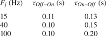
Darabi & Wygnanski (Reference Darabi and Wygnanski2004a) experimentally controlled the forced reattachment of the flow over a trailing edge flap by using a loudspeaker at the hinge line. Contrary to the present results, the time required for the flow to attach after forcing was started depended on the forcing frequency and amplitude. The minimum reattachment time obtained for a flap deflected 6 degrees over its critical angle was found to be  $tU_{\infty }/L_f = 16$, where
  $U_{\infty }$ was the free-stream velocity and
  $L_f$ the flap length. Using
  $L_f=L_b=0.42\ \textrm {m}$ and
  $U_{\infty }=U_{ref}=25\ \textrm {m}\,\textrm {s}^{-1}$, this corresponds to a time
  $t=269\ \textrm {ms}$ in our case. As can be seen in figure 20, this value is close to the time where the
  $\gamma (t)$ curves reach their asymptotes (approximately 300 ms). Darabi & Wygnanski (Reference Darabi and Wygnanski2004b) then investigated the transient separation process on the flap by abruptly stopping the loudspeaker forcing and found that the time required for separation to completely reappear was approximately 30 % larger than the time required to force the flow to attach. We conclude that the values of both time constants
  $\tau _{Off\text {--}On}$ and
  $\tau _{On\text {--}Off}$ are consistent with those of Darabi & Wygnanski (Reference Darabi and Wygnanski2004a,Reference Darabi and Wygnanskib) despite significant differences in flow configuration and forcing method. It should be noted, however, that the separation line in Darabi & Wygnanski's (Reference Darabi and Wygnanski2004a; Reference Darabi and Wygnanski2004b) experiment was essentially fixed at the flap corner.
Time traces of the transient forward-flow fraction  $\gamma (t)$ were also measured at multiple streamwise positions in order to investigate the time required between the start or stop of upstream forcing and the first indication of the TSB reaction along its length. As illustrated in figure 21(
 $a$), a time delay
  $\delta t$ was defined between
  $t=1\ \textrm {s}$, which corresponds to the start or stop of forcing, and the instant when the
  $\gamma (t)$ curve reacts to forcing. The values of
  $\delta t$ were found to be almost identical for starting or stopping sequences and are plotted in figure 21(
 $b$) as a function of the streamwise position. The streamwise distribution of
  $\delta t$ is essentially linear and hints at a convection velocity of
  $0.27U_{ref}$, which is very close to the convection velocity
  $U_c \simeq 0.30U_{ref}$ of both the naturally occurring and the PJA vortices in the shear layer. This indicates that at each streamwise position, the unforced TSB starts its deformation with the passage of the first vortex system emanating from the PJAs. Thereafter, several vortices are required for the TSB to reach its asymptotic state. As indicated in figure 20, approximately 300 ms are required for all transient effects to have disappeared when forcing is started. This time delay corresponds to the passage of 5, 12 and 30 vortex pairs for
  $F_j$ = 15, 40 and 100 Hz, respectively. Similarly, the forced TSB starts to move back to its unforced position after the passage of the last vortex pair from the PJA when forcing is stopped but requires more time to complete its motion.
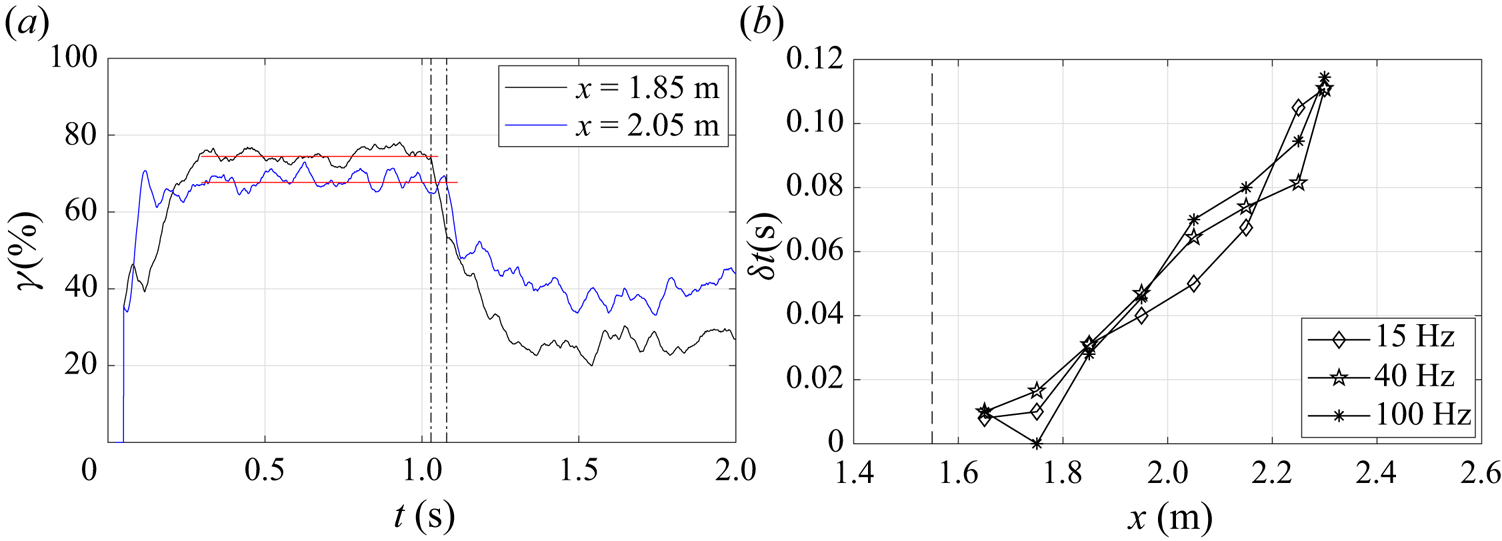
Figure 21. ( $a$) Illustration of the definition of the time delay
  $\delta t$ between
  $t=1\ \textrm {s}$ and the vertical dashed-dotted line at
  $x=1.85\ \textrm {m}$ and
  $x=2.05\ \textrm {m}$, respectively; (
 $b$) variation of
  $\delta t$ as a function of the streamwise position.
The transient response of the TSB was also investigated with ensemble-averaged PIV data at a forcing frequency of  $F_j=100\ \textrm {Hz}$ and an amplitude of
  $C_{\mu }=1.43\,\%$. For this, 30 PIV sequences of 1 s each were recorded at the most upstream PIV station. The camera recordings were synchronised to start exactly when the forcing started (Off/On sequence) or stopped (On/Off sequence). Contours of
  $\varGamma _2$ were calculated after subtracting the mean velocity
  $\bar {U}(x,y)$ of the corresponding continuous forcing case (i.e. either On or Off) from the ensemble-averaged fields.
Figure 22 illustrates a few snapshots extracted from supplementary movie 3, where the TSB reacts to a start of forcing at  $t_0$. In the first snapshot, the separation front is in its unforced position. While a few spots of
  $\left \lvert \varGamma _2\right \rvert >2/{\rm \pi}$ are visible in the field of view, they do not appear to be the signatures of the vortex structures observed in figures 15 and 17. Rather, they are interpreted as residual noise from the phase-averaging procedure. In the next snapshots, the counter-rotating vortices emanating from the PJAs at
  $F_j=100\ \textrm {Hz}$ can be seen in the two-dimensional field of view near
  $x=1.65\ \textrm {m}$ and
  $x=1.75\ \textrm {m}$. The position of the vortices is constant in this representation since the time between snapshots was chosen to be exactly six forcing periods. Between
  $t_0+60\ \textrm {ms}$ and
  $t_0+180\ \textrm {ms}$, only the counter-clockwise vortex is seen in the most downstream position (
 $x=1.75\ \textrm {m}$), again presumably because the other half of the pair is located outside of the field of view like in figure 17. In the last snapshot, however, the complete pair is observed again because the separation front is now downstream of the field of view, which results in a smaller average vertical velocity and a situation similar to that observed in figure 15. The translation of the vortices through the field of view is obvious in supplementary movie 3: each arrival of a new vortex pair slightly pushes the separation front downstream and, after 240 ms, or 24 vortex passages, the region of phase-averaged backflow is shifted downstream of the field of view. These PIV results are consistent with figure 20(
 $c$) since a downstream shift of the separation front implies an increase of forward-flow fraction at
  $x=1.75\ \textrm {m}$. Indeed, figures 19 and 20(
 $c$) indicate that
  $\gamma (t)$ still increases slightly after 240 ms and that the TD point finally settles near
  $x \simeq 1.90\ \textrm {m}$ after the disappearance of transient effects at
  $t \simeq 300\ \textrm {ms}$.
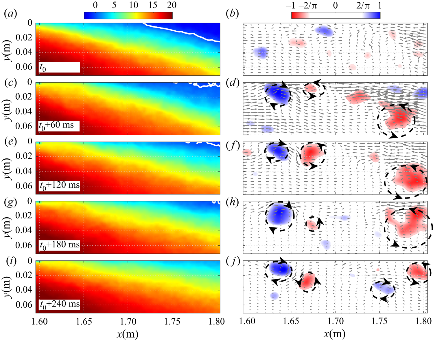
Figure 22. Illustration of the flow dynamics in PIV station 1 for a start of forcing at  $F_j=100\ \textrm {Hz}$ and
  $C_{\mu }=1.4\,\%$ with contours of phase-averaged streamwise velocity (a,c,e,g,i) and
  $\varGamma _2$ (b,d,f,h,j). Forcing is started at
  $t_0$. See also supplementary movie 3.
The stopping of upstream forcing is illustrated in figure 23 and supplementary movie 4 for the same parameters as above. The first snapshot at  $t_0$ is taken exactly when forcing is stopped. At this instant the separation front (i.e. the TD point) is located downstream of the field of view and the contour of
  $\varGamma _2$ shows the typical pair of contra-rotating vortices observed when the flow is continuously forced at
  $F_j=100\ \textrm {Hz}$ (see figures 17 and 22). In the next snapshots these vortices disappear from the field of view since forcing is stopped. Rather, the ensemble-averaging procedure produces a random contour akin to noise, which would probably have been completely eliminated with a larger number of averaging periods. Crucially, the time between snapshots is much longer in figure 23 than in figure 22, which shows that the separation front takes approximately twice as much time to come back to its original position when forcing is stopped than to move to its controlled position when forcing is started. This is consistent with the time traces of
  $\gamma (t)$ obtained with the calorimetric sensor (figure 20) and with the values of the corresponding time constants summarized in table 3.
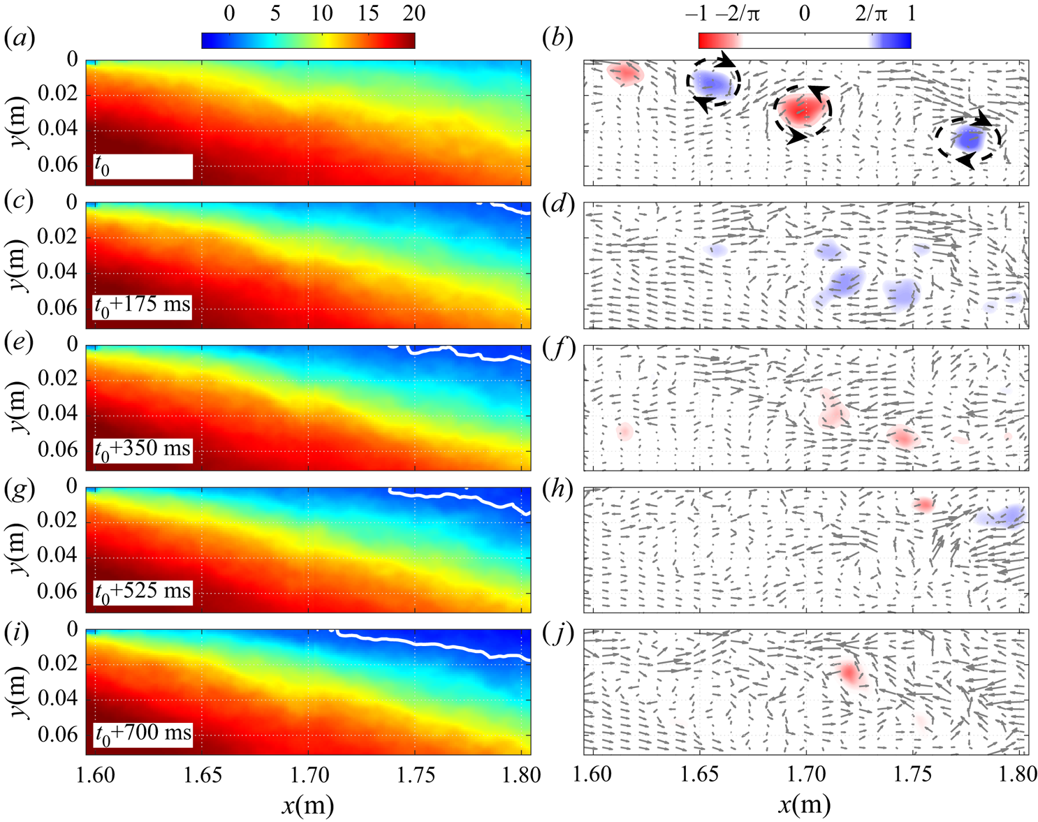
Figure 23. Illustration of the flow dynamics in PIV station 1 for a stop of forcing at  $F_j=100\ \textrm {Hz}$ and
  $C_{\mu }=1.4\,\%$ with contours of phase-averaged streamwise velocity (a,c,e,g,i) and
  $\varGamma _2$ (b,d,f,h,j). Forcing is stopped at
  $t_0$. See also supplementary movie 4.
In summary, the results presented in this section demonstrate that the TSB responds to upstream forcing with a characteristic time scale that is much larger than the forcing period of the PJAs. When forcing is started the TSB takes approximately 300 ms to reach its continuously forced state but, depending on the forcing frequency, it can take twice as long to return to its unforced state. The time traces of the transient forward-flow fraction  $\gamma (t)$ further suggest that the TSB responds to upstream perturbations like a first-order linear system with a characteristic time constant of the order of 0.1–0.2 s.
6. Discussion
The main objective of the present experiment was to investigate how periodic forcing upstream of the TSB may help understand the naturally occurring, low-frequency breathing motion already documented in this flow. Strong similarities between forcing and breathing were indeed uncovered.
(i) First, it was shown that periodic forcing in the upstream boundary layer artificially reduces the size of the TSB by pushing separation downstream and reattachment upstream. The displacement of the separation point (TD) is larger than that of the reattachment point (TR), which is consistent with what is observed when the TSB is naturally contracting and expanding at low frequency (Weiss et al. Reference Weiss, Mohammed-Taifour and Schwaab2015; Mohammed-Taifour & Weiss Reference Mohammed-Taifour and Weiss2016).
(ii) Second, the average pressure distribution measured when the TSB size is artificially modified by forcing is consistent with the model of natural low-frequency behaviour presented in figure 8. Specifically, when the TSB contracts, the average pressure is reduced near the positions of maximum and minimum pressure gradient and slightly elevated in the middle of the TSB. This behaviour is expected because a smaller TSB implies an increased pressure recovery in the separated region.
(iii) Third, when forcing is started or stopped, the separation point moves first and the reattachment thereafter. This is again similar to the low-frequency breathing, whose pressure signature is measured on average 44 ms later at
 $x=2.3\ \textrm {m}$ than at $x=1.6\ \textrm {m}$ (figure 7). The difference between this value and the time delay observed during forcing (${\simeq }110\ \textrm {ms}$, figure 21) may be explained by the different techniques used to measure the delay. Figure 7 shows the pressure signature of the breathing motion whereas figure 21 is obtained from the near-wall velocity. It is reasonable to assume that when the separation point is shifted one way or the other, changes in the global flow structure are transmitted through convection in the inviscid flow whereas the near-wall velocity only changes when turbulent structures in the shear layer reach the local measurement position. Thus, the near-wall velocity information is transmitted slower than the pressure signal.
(iv) Finally, the time constants obtained when forcing is abruptly started or stopped are strikingly similar to the characteristic time scale of the breathing motion: the largest time constant
$\tau =0.2\ \textrm {s}$ in table 3 implies a characteristic frequency $f=1/2{\rm \pi} \tau =0.8\ \textrm {Hz}$ which compares very well with the low-frequency pressure signature observed in figure 6. Furthermore, the fact that the separation and reattachment times measured by Darabi & Wygnanski (Reference Darabi and Wygnanski2004a,Reference Darabi and Wygnanskib) are consistent with ours suggests that the present results might be transferable to other flow configurations.


These findings strongly support the hypothesis formulated in § 3 that the breathing motion is a response of the TSB to turbulent fluctuations in the upstream boundary layer that affect the position of separation first and, indirectly, the position of reattachment through a global change of the pressure distribution. In effect, the TSB acts like a low-pass filter to the broadband perturbations naturally present in the upstream turbulent boundary layer, and contracts and expands with an amplitude and frequency that depends on the scale of the overall separated flow. The form of the transient forward-flow fraction curves plotted in figure 20 suggests a simple first-order linear model of the form
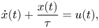 \begin{equation} \dot{x}(t)+\frac{x(t)}{\tau} = u(t), \end{equation}
where  $x$ may either represent a short-time average of the forward-flow fraction
  $\gamma$ at a specific streamwise position or of the separation or reattachment line, and where
  $u(t)$ is a forcing term linked to velocity fluctuations in the upstream boundary layer. By short-time average we mean a quantity averaged over a period longer than a typical turbulent time scale but shorter than the characteristic time scale
  $\tau$ of the separation front. In the frequency domain, (6.1) is equivalent to
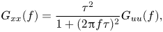 \begin{equation} G_{xx}(f) = \frac{\tau^2}{1+(2 {\rm \pi}f \tau)^2} G_{uu}(f), \end{equation}
where  $G_{xx}(f)$ and
  $G_{uu}(f)$ are the autospectral density functions of
  $x(t)$ and
  $u(t)$, respectively (Bendat & Piersol Reference Bendat and Piersol2010). This frequency-domain representation clearly illustrates the filtering character the TSB and the fact that
  $1/2{\rm \pi} \tau$ should be interpreted as some sort of cutoff frequency instead of a characteristic spectral peak.
A crude model of upstream forcing by the PJAs may be obtained by choosing
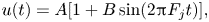 \begin{equation} u(t) = A [1+ B \sin(2 {\rm \pi}F_j t)], \end{equation}
where the model parameters  $A$ and
  $B$ depend on the forcing frequency
  $F_j$ and are chosen to match the experimental data. Equations (6.1) and (6.3) are solved in figure 24(
 $a$) for a set of parameters
  $(A,B)=(70/\tau ,1)$,
  $(85/\tau ,0.1)$, and
  $(90/\tau ,0.1)$ for
  $F_j=15$, 40 and 100 Hz, respectively. In this example,
  $x=\gamma$,
  $\tau =0.1\ \textrm {s}$, and the integration is started from
  $\gamma =50\,\%$ at
  $t=1\ \textrm {s}$. Clearly, the model matches remarkably well the experimental time traces of transient forward-flow fraction shown in figure 20. Similarly, figure 24(
 $b$) depicts the autospectral density function of
  $x$ in its standard (
 $G_{xx}$) and pre-multiplied (
 $\,f \times G_{xx}$) form when the forcing
  $u(t)$ is assumed to be white noise simulating turbulent fluctuations in the upstream boundary layer, i.e.
  $G_{uu}(f)=1$, and when the TSB time constant is
  $\tau =0.2\ \textrm {s}$. Assuming like in figure 8 that the low-frequency pressure signature consists of a back-and-forth translation of the average APG and FPG on the test surface,
  $G_{xx}$ can also be interpreted as a wall-pressure p.s.d. Here also, the model agrees very well with the low-frequency character of wall-pressure fluctuations measured at
  $x=1.60\ \textrm {m}$ and presented in figure 6. Finally, figure 25 shows the p.s.d.s of streamwise velocity fluctuations measured with a hot-wire probe at a wall-normal position
  $y \simeq \delta$ in the unforced TSB, where
  $\delta$ is the 99 % boundary-layer thickness. The appropriate resolution at low frequencies was obtained by integrating the signal for 300 s. Two streamwise positions are considered:
  $x=1.45\ \textrm {m}$ is at the very beginning of the APG and
  $x=1.60\ \textrm {m}$ is at ID, close to the position of maximum low-frequency pressure signature (see figure 5). Above 3 Hz, the p.s.d.s at both positions are very similar but below 3 Hz, the amplitude is almost an order of magnitude higher at
  $x=1.60\ \textrm {m}$. This difference occurs because of the breathing motion in the unforced TSB, whose low-frequency signature can be observed in both wall-pressure and velocity signals (Mohammed-Taifour & Weiss Reference Mohammed-Taifour and Weiss2016). Also shown in the figure is the output
  $G_{xx}$ of (6.2) applied to the p.s.d. measured at
  $x=1.45\ \textrm {m}$ and scaled to fit the lowest-frequency value of the
  $x=1.60\ \textrm {m}$ p.s.d. It can be seen that at
  $x=1.60\ \textrm {m}$, both
  $G_{xx}$ and
  $G_{uu}$ follow the same trend at low frequencies, which further supports the validity of a low-pass filter model transforming a broadband turbulent signal into a low-frequency contraction and expansion of the TSB. We conclude that the simple first-order model (6.1)/(6.2), although purely heuristic, offers a good approximation of both the TSB response to artificial periodic forcing and of its natural low-frequency unsteadiness.
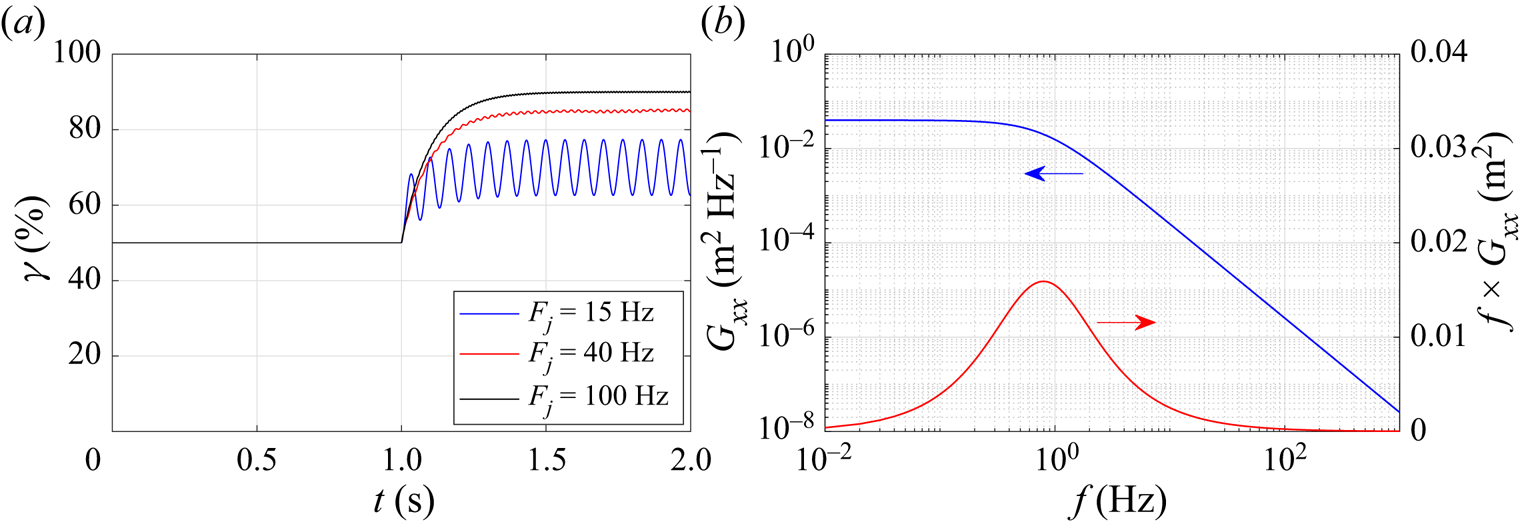


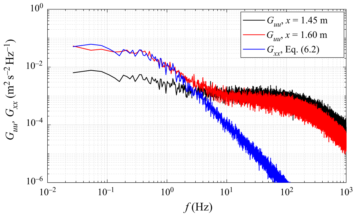
Figure 25. The p.s.d.s of streamwise velocity fluctuations ( $G_{uu}$) measured at
  $x=1.45\ \textrm {m}$ and
  $x=1.60\ \textrm {m}$ (
 $y \simeq \delta$) and scaled output of first-order model
  $G_{xx}$ applied to the
  $x=1.45\ \textrm {m}$ data with
  $\tau = 0.2\ \textrm {s}$.
Interestingly, a first-order model similar to (6.1) was devised by Plotkin (Reference Plotkin1975) to relate the low-frequency shock oscillations observed in turbulent SBLI flows to broadband velocity fluctuations in the upstream boundary layer. Plotkin's model is compressible in nature and assumes that the velocity of the separation shock in a turbulent SBLI is the superposition of a random forcing and a restoring velocity that is proportional to the displacement of the shock. These assumptions naturally lead to a first-order equation similar to (6.1), where  $x$ is the position of the separation shock. Touber & Sandham (Reference Touber and Sandham2011) subsequently derived a low-order stochastic model for impinging shock SBLIs that is mathematically equivalent to Plotkin's model. On the basis of this model, they argued that the origin of the low-frequency unsteadiness in such SBLIs is caused by the inherent dynamics of the boundary layer and shock system which act as a low-pass filter to incoming turbulent perturbations. Poggie et al. (Reference Poggie, Bisek, Kimmel and Stanfield2015) demonstrated that this simple model is consistent with wall-pressure spectra obtained in a large number of SBLI flows generated in wind-tunnel experiments, flight tests and numerical simulations. The success of a similar first-order model in our low-Mach-number experiment suggests that it may be the separation front, and not necessarily the separation shock, that acts as a filter. Such a conclusion would not invalidate existing results in SBLI flows since in all likelihood the separation shock would follow a slowly moving separation front.
LeFloc'h et al. (Reference LeFloc'h, Weiss, Mohammed-Taifour and Dufresne2020) investigated the low-frequency breathing of a family of TSBs generated in the same wind tunnel as the one used in the present experiment by varying the streamwise position of the FPG in figure 1. By moving the FPG upstream, smaller TSBs could be generated with the same APG. It was found that the pressure and velocity signatures of the low-frequency breathing were smaller when the TSB size was reduced. In the framework of the present model of low-frequency breathing, this would mean that the low-frequency motion of the separation front is smaller for a shorter TSB, which is expected since the most downstream position of separation is necessarily bounded by the average FPG. Thus, we expect that the amplitude of the low-frequency breathing will increase with the streamwise extent of the TSB since the separation front may move over a larger distance. This is consistent with the recent DNS results of Wu et al. (Reference Wu, Meneveau and Mittal2020), who observed low-frequency unsteadiness in a large TSB generated with a suction-only boundary condition but not in smaller TSB obtained with a suction-and-blowing condition. On the other hand, the reattachment position in Reference Wu, Meneveau and MittalWu et al.'s (Reference Wu, Meneveau and Mittal2020) suction-only TSB appeared to move over a larger distance than the separation front. This is in contrast with the present configuration and may possibly be explained by the absence of an FPG in the aft part of their TSB and the resulting reattachment through turbulent diffusion only. Furthermore, the absence of any low-frequency breathing with the suction-and-blowing configuration of Wu et al. (Reference Wu, Meneveau and Mittal2020), which is not much different than the present configuration, remains unexplained.
It is also interesting to compare the proposed mechanism of low-frequency unsteadiness in the present TSB to a mechanism already formulated to explain the flapping motion of laminar separation bubbles. As suggested by the results of Marxen & Henningson (Reference Marxen and Henningson2011) and Michelis et al. (Reference Michelis, Yarusevych and Kotsonis2017), the low-frequency flapping in a LSB may be characterised by both a downstream shift of the separation point and an upstream shift of reattachment. Therefore, in effect, this motion could also be described as ‘breathing’, like in the present TSB. Crucially, however, in a LSB the separation point moves much less than the reattachment point, which explains why the shear layer may be seen as ‘flapping’, as if the separation point were fixed. Another striking difference between TSB and LSB unsteadiness is that in a LSB, the (low-frequency) reattachment point moves first and is followed by the separation point (Dovgal & Kozlov Reference Dovgal and Kozlov1995; Marxen & Henningson Reference Marxen and Henningson2011). A reduction in LSB size might occur when incoming disturbances in the free stream increase in the most unstable range of frequencies of the shear layer. This triggers transition earlier and pushes reattachment upstream, which in turn provokes a global change of the pressure distribution and a downstream shift of the separation point through viscous–inviscid interaction. The smaller bubble is then more stable to incoming disturbances, which results in a feedback loop (Marxen & Henningson Reference Marxen and Henningson2011; Michelis et al. Reference Michelis, Yarusevych and Kotsonis2017; Marxen Reference Marxen2020). In the present TSB, upstream disturbances from the turbulent boundary layer affect separation first. The (low-frequency) reattachment point follows later through a viscous–inviscid interaction that provokes a global change of the pressure distribution, and the TSB size is modulated.
One may also note that in a geometry-induced TSB, the mechanism of low-frequency unsteadiness (usually referred to as ‘flapping’ in the literature) must be different than in the present pressure-induced TSB because in the former case the separation point is necessarily fixed. As mentioned above, most existing studies on geometry-induced TSBs indicate that forcing strongly influences the development of the shear layer while in the present case, the shear layer remains relatively unaffected. It is therefore expected that the flapping of geometry-induced TSBs is also linked to the development of the shear layer.
Finally, we briefly come back to the assumption of quasi-two-dimensionality introduced in § 2.4. As can be seen in the oil-film visualizations of figure 3, despite a constant forcing amplitude in the spanwise direction, the separation line is strongly curved when the actuators are placed at  $x=1.55\ \textrm {m}$. This corresponds to the majority of forced cases discussed in this article. Thus, strictly speaking, the results are only valid on the test-section centreline and it is legitimate to ask what would be different in the absence of corner effects. While it is impossible to be certain without a dedicated investigation, the most likely consequence would be an even stronger effect of forcing on the TSB size. Indeed, the motion of the TD point on the centreline appears to be constrained by the sidewalls. If this constraint were relaxed, it is probable that the TD point would move even further for a specified forcing input. Thus, in a way, the effect of forcing on the TSB size may be considered as conservative in the present experiment. On the other hand, the potential influence of corner effects on the time scales investigated in this work remains unknown. In this respect, highly resolved numerical simulations, where sidewall effects can be artificially removed, would be very welcome to further investigate this flow configuration.
7. Conclusion
The response of a large pressure-induced TSB to periodic forcing was investigated in this work in an attempt to elucidate the mechanism responsible for the low-frequency breathing motion already documented in the unforced flow. The TSB was generated on a flat test surface by the APG-induced separation of a turbulent boundary layer followed by its FPG-induced reattachment. Both continuous and transient forcing using pulsed-jet actuators were considered, and the flow was probed using steady and unsteady pressure transducers, a MEMS calorimetric shear-stress sensor and high-speed PIV.
Results from the continuous forcing experiments indicate that the size of the TSB can be artificially reduced by periodic forcing in the upstream boundary layer. Forcing pushes the TD point downstream and the TR point upstream, thus leading to a contraction of the original TSB. As a consequence, the streamwise distributions of forward-flow fraction and average pressure both narrow and the turbulent stresses in the shear layer decrease. The size of the TSB decreases with increasing forcing amplitude and the range of most effective frequencies that lead to the smallest TSB is 3 to 7 times the natural shedding frequency. Regardless of the chosen frequency and amplitude, periodic forcing appears to mostly influence the flow physics near separation, while the aft part of the shear layer in the reattachment region remains relatively unaffected. This suggests that the motion of the reattachment point (TR) occurs because of a redistribution of the global flow structure caused by the downstream shift of the separation point (TD) and not because of an enhancement of vortex merging in the shear layer. In this respect, the effect of forcing appears to be different than in geometry-induced TSBs, where forcing is known to strongly affect the development of the shear layer. Transient forcing experiments, during which the periodic forcing is either abruptly started or stopped, further demonstrate that the TSB responds to upstream forcing with a characteristic frequency that is much smaller than the forcing frequency of the PJAs, but that is of the same order of magnitude as that of the natural low-frequency breathing motion.
Overall, the present results support a mechanism where the low-frequency breathing motion is a response of the TSB to upstream turbulent perturbations. The TSB appears to behave like a first-order low-pass filter that converts the broadband fluctuations present in the incoming turbulent boundary layer into a low-frequency, large-scale fluctuation of the separation and reattachment fronts, thus leading to a contraction and expansion of the TSB. The upstream perturbations affect the position of separation first and, indirectly, the position of reattachment through a low-frequency, global redistribution of the pressure and velocity fields (viscous–inviscid interaction). In that sense, the mechanism bears some resemblance with the low-frequency flapping of LSBs, although in the latter case the reattachment moves first and is followed by the separation point (Marxen Reference Marxen2020). The proposed mechanism of low-frequency unsteadiness must also be different than in geometry-induced TSBs where the separation point is fixed on the test surface.
In addition to the conclusions obtained with respect to the mechanism of low-frequency breathing, results from the continuous forcing experiments also offer new insights into active separation control with PJAs. Specifically, the phase-averaged PIV results demonstrate that PJAs operate by generating strong starting vortices that are associated with a downstream shift of the separation front. Given the large parameter space that governs the use of PJAs, further research appears necessary to optimize their usage for AFC purposes.
Supplementary movies
Supplementary movies are available at https://doi.org/10.1017/jfm.2021.77.
Acknowledgements
The support of A. LeFloc'h and E. Jondeau during the experiments is greatly appreciated.
Funding
This work was supported by the Natural Sciences and Engineering Research Council of Canada and the Canadian Foundation for Innovation.
Declaration of interests
The authors report no conflict of interest.


