1 Introduction
1.1 Resonant dynamics of coupled fluid–structure system
Unsteady flows involving fluid–structure interactions (FSIs) are widespread in numerous engineering applications, and their fundamental understanding poses serious challenges due to the richness and complexity of nonlinear coupled physics. Even a simple configuration of a coupled fluid–structure system can exhibit complex spatial-temporal dynamics and synchronization as functions of physical parameters and geometric variations. Synchronization is a general nonlinear physical phenomenon in fluid–structure systems whereby the coupled system has an intrinsic ability to lock at a preferred frequency and amplitude. For example, when a bluff body immersed in a cross-flow is flexible or mounted elastically, there exists a strong coupling between the bluff body and the vortices forming in its wake. In particular, as the natural frequency (
 $f_{n}$
) of the bluff body approaches the frequency of the wake system, typically the frequency of vortex shedding (
$f_{n}$
) of the bluff body approaches the frequency of the wake system, typically the frequency of vortex shedding (
 $f_{vs}$
), the wake–body frequency lock-in behaviour is observed which plays a crucial role in establishing the synchronization. During this frequency lock-in, the bluff body experiences a large self-limiting vibration (Khalak & Williamson Reference Khalak and Williamson1999) and a dynamical equilibrium between the energy transfer and dissipation exists. This synchronization has been a major topic of research to understand the mechanism of this energy transfer and the sustenance of self-excited vibrations. In the present study we consider a prismatic square geometry to understand the wake–body synchronization and to perform the decomposition of wake dynamics during the FSI.
$f_{vs}$
), the wake–body frequency lock-in behaviour is observed which plays a crucial role in establishing the synchronization. During this frequency lock-in, the bluff body experiences a large self-limiting vibration (Khalak & Williamson Reference Khalak and Williamson1999) and a dynamical equilibrium between the energy transfer and dissipation exists. This synchronization has been a major topic of research to understand the mechanism of this energy transfer and the sustenance of self-excited vibrations. In the present study we consider a prismatic square geometry to understand the wake–body synchronization and to perform the decomposition of wake dynamics during the FSI.
The phenomenon of frequency lock-in is a major concern in offshore, marine and aeronautical engineering, whereby structures are designed to avoid the large-amplitude vibrations by selecting optimal system parameters (e.g. geometric dimensions, stiffness, damping) and/or installing active and passive devices to control the intensity of FSI. In particular, several studies have been conducted with the purpose of controlling the wake–body interaction via passive and active devices (Guan et al. Reference Guan, Narendran, Miyanawala, Ma and Jaiman2017; Law & Jaiman Reference Law and Jaiman2017; Narendran et al. Reference Narendran, Guan, Ma, Choudhary, Hussain and Jaiman2018) with the physical insight based on the reliance of frequency lock-in on the large-scale features of the wake. In fact, these studies were found to be remarkably successful in suppressing large-amplitude motion of the body by avoiding the interaction between the major organized features of the wake. However, the mechanism of the interactions among the wake features and their impact on the free motion of the bluff body is not properly explained. Moreover, the available experimental and numerical data can be used to provide a deeper understanding and a new insight into the kinematics and dynamics of synchronized wake–body interaction. This paper aims to explain how different organized flow features (i.e. near-wake structures) amplify the bluff body motion and sustain the energy transfer from the fluid flow to the vibrating body. Specifically, we examine the formation of the dominant coherent structures and their nonlinear interactions during the wake–body synchronization.
The vortex shedding pattern is undoubtedly the most prominent wake feature behind a bluff body. It is present in almost all of the separated wake flows and has been studied extensively in the literature. This primary wake feature begins at a much lower
 $Re$
: for example, in a circular cylinder wake, at
$Re$
: for example, in a circular cylinder wake, at
 $Re\approx 49$
, it exhibits a classical Kármán vortex street and develops the three-dimensional vorticity patterns when
$Re\approx 49$
, it exhibits a classical Kármán vortex street and develops the three-dimensional vorticity patterns when
 $Re\gtrsim 190$
. In addition to the vortex street, a free shear layer (not attached to a solid surface) is an important dynamical feature that represents a separating high-gradient layer behind a bluff body, and it arises between the higher free stream velocity and the smaller velocity occurring in the wake region. The shear layer behaves likes a perturbed vortex sheet and is highly sensitive and unstable to small disturbances, giving rise to alternating thickening and thinning of the vortex sheet. The characteristic vortex structures develop when shear layer thickening occurs. For the unsteady two-dimensional regime (
$Re\gtrsim 190$
. In addition to the vortex street, a free shear layer (not attached to a solid surface) is an important dynamical feature that represents a separating high-gradient layer behind a bluff body, and it arises between the higher free stream velocity and the smaller velocity occurring in the wake region. The shear layer behaves likes a perturbed vortex sheet and is highly sensitive and unstable to small disturbances, giving rise to alternating thickening and thinning of the vortex sheet. The characteristic vortex structures develop when shear layer thickening occurs. For the unsteady two-dimensional regime (
 $49\leqslant Re\leqslant 190$
for a circular cylinder) the roll-up of the shear layers with the formation of the vortex street can be observed (Williamson Reference Williamson1996). These shear layers are predominantly elongated in the streamwise direction and have a high gradient in the cross-flow direction. Behind a moving or stationary bluff body, the region of a recirculating region with the rotational flow is present due to the fluid viscosity. Owing to nonlinear flow separation and turbulence, complex interactions occur in the mean recirculation region, which is also referred to as the near-wake bubble. Several previous studies have explored the dynamical features inside the wake region (with the vortex shedding and the shear layer) using experimental (Cantwell & Coles Reference Cantwell and Coles1983), numerical (Braza, Chassaing & Minh Reference Braza, Chassaing and Minh1986) and both (Bearman Reference Bearman1997; Dong et al.
Reference Dong, Karniadakis, Ekmekci and Rockwell2006) techniques. In the present analysis we consider the near-wake bubble as a distinct feature from the vortex street and the shear layer. The near-wake region accounts for the complex interactions of the mean circulation region, which can be considered as a general feature and can be identified separately from the other two features. Hence, we divide the wake into three dominant organized coherent structures: the vortex street, the shear layer, and the near-wake bubble. These organized features have an intrinsic dynamics of their own and influence each other in a nonlinear manner over a wide range of space and time scales. A primary goal of this paper is to employ low-dimensional models to extract the organized wake features and to examine their roles during the wake–body synchronization.
$49\leqslant Re\leqslant 190$
for a circular cylinder) the roll-up of the shear layers with the formation of the vortex street can be observed (Williamson Reference Williamson1996). These shear layers are predominantly elongated in the streamwise direction and have a high gradient in the cross-flow direction. Behind a moving or stationary bluff body, the region of a recirculating region with the rotational flow is present due to the fluid viscosity. Owing to nonlinear flow separation and turbulence, complex interactions occur in the mean recirculation region, which is also referred to as the near-wake bubble. Several previous studies have explored the dynamical features inside the wake region (with the vortex shedding and the shear layer) using experimental (Cantwell & Coles Reference Cantwell and Coles1983), numerical (Braza, Chassaing & Minh Reference Braza, Chassaing and Minh1986) and both (Bearman Reference Bearman1997; Dong et al.
Reference Dong, Karniadakis, Ekmekci and Rockwell2006) techniques. In the present analysis we consider the near-wake bubble as a distinct feature from the vortex street and the shear layer. The near-wake region accounts for the complex interactions of the mean circulation region, which can be considered as a general feature and can be identified separately from the other two features. Hence, we divide the wake into three dominant organized coherent structures: the vortex street, the shear layer, and the near-wake bubble. These organized features have an intrinsic dynamics of their own and influence each other in a nonlinear manner over a wide range of space and time scales. A primary goal of this paper is to employ low-dimensional models to extract the organized wake features and to examine their roles during the wake–body synchronization.
1.2 Low-dimensional models for wake features
To extract the large-scale organized/coherent wake features, it is required to decompose the dynamic flow fields by scales into different constituent kinematical regions. The concept of decomposition by scale has been prevalent in much fluid dynamics research ranging from a low-dimensional projection of flow field to turbulence modelling by ensemble averaging, temporal or spatial averaging. A general decomposition technique can be considered to separate the space-time data for representing different characteristics of the field. For example, the proper orthogonal decomposition (POD) extracts the most energetic modes in an optimal way and provides structural information from the wake data. The POD is a popular method for constructing low-order modelling from the data (Holmes Reference Holmes2012), and it is often referred to as the Karhunen–Loève expansion or the principal component analysis. The key idea behind the Karhunen–Loève expansion is to determine a low-dimensional affine subspace from the high-dimensional data while retaining the important dynamics of the full-order model. After the determination of the best approximating low-dimensional subspace, a Galerkin projection is employed to project the dynamics onto it. In this work, we will employ this low-dimensional subspace projection procedure for extracting the large-scale wake features from the high-dimensional flow dynamics data.
In the context of the present study, the POD-Galerkin projection method is quite attractive for capturing the synchronized dynamics such as the vortex shedding and the near-wake interactions (Noack et al. Reference Noack, Afanasiev, Morzyński, Tadmor and Thiele2003; Rempfer Reference Rempfer2003). In addition, it has been the dominant empirical model reduction technique incorporated for the standard flow around a stationary circular cylinder for the past few decades. For example, in a pioneering study, Deane et al. (Reference Deane, Kevrekidis, Karniadakis and Orszag1991) reproduced the flow dynamics of the laminar wake by employing merely an eight-dimensional model, which was further generalized to generate reduced spaces for a three-dimensional velocity field by Ma & Karniadakis (Reference Ma and Karniadakis2002) using direct numerical simulation data. In general, the empirical POD-Galerkin models are capable of reconstructing the reference dynamics with higher accuracy than the standalone mathematical or physical Galerkin methods, while capturing the physically most significant modes (Noack et al. Reference Noack, Afanasiev, Morzyński, Tadmor and Thiele2003). With regard to the applications of the POD-Galerkin models to bluff body wake flows, these modes correspond to the organized wake features such as the vortex street, the shear layer and the near-wake bubble. Although there is a significant body of work on the wake modes for a stationary cylinder, they have not been examined in the context of wake–body interaction and the lock-in process. One of the contributions of the present study is to build some connections between the wake features and the lock-in process. During the lock-in/synchronization, the vibrating body undergoes a highly nonlinear wake–body interaction with self-sustained oscillations.
In the early studies of POD application to fluid flows (Lumley Reference Lumley, Yaglom and Tatarsky1967; Sirovich Reference Sirovich1987), the dynamic flow field is reconstructed by a linear combination of the most significant modes. Hence, it has a considerable local error in the highly nonlinear regions of the organized wake motions and the evaluation of the projected nonlinear term has a direct dependence on the large dimension of the original system. This problem is mitigated to a certain extent by increasing the sampling frequency and/or refining the spatial discretization of the reference data. However, these temporal and spatial refinements increase the cost of model reduction without directly addressing the nonlinear nature of the flow. To introduce the nonlinearity, Petrov–Galerkin projections to the Navier–Stokes formulation or Koopman operators are incorporated in some studies (Rowley & Dawson Reference Rowley and Dawson2017). Instead of such explicit models, we employ the recently developed discrete empirical interpolation method (DEIM; Chaturantabut & Sorensen Reference Chaturantabut and Sorensen2009) for dynamical systems, which reconstructs the fields as a nonlinear combination of the POD modes. Apart from the POD basis subspace, the method relies on the additional POD basis to enrich the low-rank approximation of the nonlinear terms. In the POD-DEIM, a set of best points are selected using a greedy selection and the reconstruction is based on the time history of the field data of those points. This reduces the computational cost of the technique and further allows nonlinearities to be captured during the reconstruction of highly nonlinear dynamic wake fields (Rowley & Dawson Reference Rowley and Dawson2017).
1.3 Contributions and organization
For the past few decades, studies on the low-dimensional decomposition of wake features have primarily been focused on flow past stationary bodies, particularly on a circular cylinder (Deane et al. Reference Deane, Kevrekidis, Karniadakis and Orszag1991; Noack et al. Reference Noack, Afanasiev, Morzyński, Tadmor and Thiele2003; Rowley & Dawson Reference Rowley and Dawson2017; Taira et al. Reference Taira, Brunton, Dawson, Rowley, Colonius, Mckeon, Schmidt, Gordeyev, Theofilis and Ukeiley2017). This may be due to the fact that the flow exhibits a diverse set of complex phenomena despite its simple geometry. However, very few studies (Liberge & Hamdouni Reference Liberge and Hamdouni2010; Yao & Jaiman Reference Yao and Jaiman2017) are found on unsteady FSI systems. Here we provide a modal reduction study on the flow past a freely vibrating sharp-cornered square cylinder with two-degrees-of-freedom motions. We consider a configuration of a square cylinder for our numerical study of wake–body synchronization because this configuration has fixed and perfectly symmetric separation points at the leading sharp corners, because entirely resonance-induced lock-in exists (Yao & Jaiman Reference Yao and Jaiman2017). The physical investigation is general for any fluid–structure system involving the interaction dynamics of flexible structures with an unsteady wake–vortex system. We hypothesize that the solution space of wake–body interaction attracts a low-dimensional manifold, which allows construction of a set of basis vectors for a low-dimensional representation of the high-dimensional space. The low-dimensional subspace is constructed by means of the samples collected from the high-dimensional solutions via projection-based model order reduction. We utilize the linear and nonlinear POD-based reduced-order reconstructions to understand the most significant features in the wake flow.
To extract the modes for the dynamics of wake–body synchronization, the POD in conjunction with the nonlinear POD-DEIM is applied to a set of samples collected from the full-order simulations. We exploit the POD modes obtained to answer the following intriguing questions that are prevalent in the field of fluid mechanics: (i) How do the large-scale features contribute to the unsteady forces acting on the bluff body? (ii) How do the wake features interact when the structural frequency and vortex shedding frequency are locked in, such that the vortices remain very energetic even the fluid has transferred energy to the structure? (iii) Will the wake and bluff body undergo synchronized motion below the critical
 $Re$
due to the structural flexibility? (iv) What role does the wake turbulence play when we attempt to decompose the wake into its large-scale features? In relation to (i), we quantify the force contribution from each wake feature mode to the streamwise (drag) and transverse (lift) forces and explain the observed variation. We further investigate the modal contribution of different wake features in the pre-lock-in, lock-in and post-lock-in regimes and propose a cycle explaining the sustenance of lock-in phenomena of the wake–body synchronization. We then explore the below-critical-
$Re$
due to the structural flexibility? (iv) What role does the wake turbulence play when we attempt to decompose the wake into its large-scale features? In relation to (i), we quantify the force contribution from each wake feature mode to the streamwise (drag) and transverse (lift) forces and explain the observed variation. We further investigate the modal contribution of different wake features in the pre-lock-in, lock-in and post-lock-in regimes and propose a cycle explaining the sustenance of lock-in phenomena of the wake–body synchronization. We then explore the below-critical-
 $Re$
flows to examine whether the bluff body and the wake can undergo synchronization via flexibility-induced unsteadiness. Finally, we apply POD decomposition to the three-dimensional flow at moderate
$Re$
flows to examine whether the bluff body and the wake can undergo synchronization via flexibility-induced unsteadiness. Finally, we apply POD decomposition to the three-dimensional flow at moderate
 $Re=22\,000$
, whereas the wake is fully turbulent after flow separation. A well-established dynamic large-eddy simulation is employed for generating full-order data for the turbulent wake. At this sub-critical Reynolds number, we explore the role of turbulence during the reconstruction of flow-field data and extend the wake–body synchronization cycle to the turbulent flow.
$Re=22\,000$
, whereas the wake is fully turbulent after flow separation. A well-established dynamic large-eddy simulation is employed for generating full-order data for the turbulent wake. At this sub-critical Reynolds number, we explore the role of turbulence during the reconstruction of flow-field data and extend the wake–body synchronization cycle to the turbulent flow.
The paper is structured as follows. In § 2 we briefly review the full-order model (FOM) for the coupled fluid–structure system, which follows by the formulation of modal reduction via linear POD and nonlinear POD-DEIM. Section 3 discusses the problem set-up and the mesh convergence study performed for the full-order analysis. In § 4 the reduced-order reconstruction of fluid fields using the linear and nonlinear POD methods is presented together with the analysis on the role of wake features in generating the forces. In § 5, the mode energy contributions from different flow features under lock-in conditions are investigated and a self-sustaining cycle is proposed to explain the wake interaction with the bluff body. Section 6 investigates the wake–body synchronization phenomenon at below critical
 $Re$
. Section 7 explores the application of modal decomposition for moderate-
$Re$
. Section 7 explores the application of modal decomposition for moderate-
 $Re$
flows and extends the proposed wake interaction cycle to the turbulent flow. Concluding remarks and the main results of the present study are provided in § 8.
$Re$
flows and extends the proposed wake interaction cycle to the turbulent flow. Concluding remarks and the main results of the present study are provided in § 8.
2 Numerical methodology
We first briefly summarize our high-dimensional FOM to simulate the coupled fluid–body interaction using the incompressible Navier–Stokes equations and the rigid body dynamics.
2.1 Full-order model for fluid–body interaction
We employ a variational formulation based on the arbitrary Lagrangian–Eulerian (ALE) to solve the following coupled fluid–body system:
 $$\begin{eqnarray}\displaystyle & \displaystyle \unicode[STIX]{x1D70C}^{f}\frac{\unicode[STIX]{x2202}\boldsymbol{u}^{f}}{\unicode[STIX]{x2202}t}+\unicode[STIX]{x1D70C}^{f}(\boldsymbol{u}^{f}-\boldsymbol{w})\boldsymbol{\cdot }\unicode[STIX]{x1D735}\boldsymbol{u}^{f}=\unicode[STIX]{x1D735}\boldsymbol{\cdot }\unicode[STIX]{x1D748}^{f}+\boldsymbol{b}^{f}\quad \text{on }\unicode[STIX]{x1D6FA}^{f}(t), & \displaystyle\end{eqnarray}$$
 $$\begin{eqnarray}\displaystyle & \displaystyle \unicode[STIX]{x1D735}\boldsymbol{\cdot }\boldsymbol{u}^{f}=0\quad \text{on }\unicode[STIX]{x1D6FA}^{f}(t), & \displaystyle\end{eqnarray}$$
 $$\begin{eqnarray}\displaystyle & \displaystyle \boldsymbol{M}\frac{\unicode[STIX]{x2202}\boldsymbol{u}^{s}}{\unicode[STIX]{x2202}t}+\boldsymbol{C}\boldsymbol{u}^{s}+\boldsymbol{K}(\unicode[STIX]{x1D753}^{s}(\boldsymbol{z}_{0},t)-\boldsymbol{z}_{0})=\boldsymbol{F}^{s}\quad \text{on }\unicode[STIX]{x1D6FA}^{s}, & \displaystyle\end{eqnarray}$$
where superscripts
 $f$
and
$f$
and
 $s$
denotes the fluid and structural domains, and
$s$
denotes the fluid and structural domains, and
 $\unicode[STIX]{x1D6FA}^{f}(t)$
and
$\unicode[STIX]{x1D6FA}^{f}(t)$
and
 $\unicode[STIX]{x1D6FA}^{s}$
represent the fluid and solid domains, respectively. Here
$\unicode[STIX]{x1D6FA}^{s}$
represent the fluid and solid domains, respectively. Here
 $\unicode[STIX]{x1D70C}^{f}$
is the fluid density,
$\unicode[STIX]{x1D70C}^{f}$
is the fluid density,
 $\boldsymbol{u}^{f}$
and
$\boldsymbol{u}^{f}$
and
 $\boldsymbol{w}$
are the fluid and mesh velocities at a spatial point
$\boldsymbol{w}$
are the fluid and mesh velocities at a spatial point
 $\boldsymbol{x}\in \unicode[STIX]{x1D6FA}^{f}(t)$
, and
$\boldsymbol{x}\in \unicode[STIX]{x1D6FA}^{f}(t)$
, and
 $\boldsymbol{b}^{f}$
denotes the body force in the fluid domain. For the structural system,
$\boldsymbol{b}^{f}$
denotes the body force in the fluid domain. For the structural system,
 $\boldsymbol{M}$
,
$\boldsymbol{M}$
,
 $\boldsymbol{C}$
and
$\boldsymbol{C}$
and
 $\boldsymbol{K}$
are the mass, damping and stiffness matrices of the bluff body and
$\boldsymbol{K}$
are the mass, damping and stiffness matrices of the bluff body and
 $\boldsymbol{F}^{s}$
is the external force acting on the body. The function
$\boldsymbol{F}^{s}$
is the external force acting on the body. The function
 $\unicode[STIX]{x1D753}^{s}(\boldsymbol{z}_{0},t)$
maps the initial position vector of the centre of mass (
$\unicode[STIX]{x1D753}^{s}(\boldsymbol{z}_{0},t)$
maps the initial position vector of the centre of mass (
 $\boldsymbol{z}_{0}$
) to its position at time
$\boldsymbol{z}_{0}$
) to its position at time
 $t$
, and
$t$
, and
 $\unicode[STIX]{x1D748}^{f}$
is the Cauchy stress tensor for a Newtonian fluid given by
$\unicode[STIX]{x1D748}^{f}$
is the Cauchy stress tensor for a Newtonian fluid given by
 $$\begin{eqnarray}\unicode[STIX]{x1D748}^{f}=-p\boldsymbol{I}+\unicode[STIX]{x1D707}^{f}(\unicode[STIX]{x1D735}\boldsymbol{u}^{f}+(\unicode[STIX]{x1D735}\boldsymbol{u}^{f})^{\text{T}}),\end{eqnarray}$$
where
 $p$
is the fluid pressure. In addition to the initial conditions and the standard Neumann/Dirichlet conditions, the coupled system incorporates the velocity and traction continuity conditions at the fluid–body interface
$p$
is the fluid pressure. In addition to the initial conditions and the standard Neumann/Dirichlet conditions, the coupled system incorporates the velocity and traction continuity conditions at the fluid–body interface
 $\unicode[STIX]{x1D6E4}$
as follows:
$\unicode[STIX]{x1D6E4}$
as follows:
 $$\begin{eqnarray}\displaystyle & \displaystyle \boldsymbol{u}^{f}(t)=\boldsymbol{u}^{s}(t), & \displaystyle\end{eqnarray}$$
 $$\begin{eqnarray}\displaystyle & \displaystyle \int _{\unicode[STIX]{x1D6E4}(t)}\unicode[STIX]{x1D748}^{f}(\boldsymbol{x},t)\boldsymbol{\cdot }\boldsymbol{n}\,\text{d}\unicode[STIX]{x1D6E4}+\boldsymbol{F}^{s}=\mathbf{0}, & \displaystyle\end{eqnarray}$$
where
 $\boldsymbol{n}$
is the outer normal to the fluid–body interface. The above fluid–body interface conditions are satisfied by the body-conforming Eulerian–Lagrangian treatment, which provides accurate modelling of the boundary layer and the vorticity generation over a moving body. While (2.1)–(2.3) of the coupled fluid–body system are directly solved for low-
$\boldsymbol{n}$
is the outer normal to the fluid–body interface. The above fluid–body interface conditions are satisfied by the body-conforming Eulerian–Lagrangian treatment, which provides accurate modelling of the boundary layer and the vorticity generation over a moving body. While (2.1)–(2.3) of the coupled fluid–body system are directly solved for low-
 $Re$
flows, we consider the well-established dynamic subgrid-scale model for high-
$Re$
flows, we consider the well-established dynamic subgrid-scale model for high-
 $Re$
turbulent flow. The spatially filtered Navier–Stokes and continuity equations are solved in the variational form. Details of the dynamic subgrid-scale model are provided in Jaiman, Guan & Miyanawala (Reference Jaiman, Guan and Miyanawala2016a
).
$Re$
turbulent flow. The spatially filtered Navier–Stokes and continuity equations are solved in the variational form. Details of the dynamic subgrid-scale model are provided in Jaiman, Guan & Miyanawala (Reference Jaiman, Guan and Miyanawala2016a
).
The weak variational form of (2.1) is discretized in space using equal-order isoparametric finite elements for the fluid velocity and pressure. In the present study, we utilize the nonlinear partitioned staggered procedure for the full-order simulations of FSI (Jaiman, Pillalamarri & Guan Reference Jaiman, Pillalamarri and Guan2016b ). The motion of the structure is driven by the traction forces exerted by the fluid flow, whereby the structural motion predicts the new interface position and the geometry changes for the moving fluid domain at each time step. The movements of the internal ALE fluid nodes are updated such that the mesh quality does not deteriorate as the motion of the solid structure becomes large. To extract the transient flow characteristics, we solve the Navier–Stokes equations at discrete time steps, which leads to a sequence of linear systems of equations via Newton–Raphson-type iterations. We employ the conjugate gradient, with a diagonal preconditioner for the symmetric matrix arising from the pressure projection and the standard generalized minimal residual solver based on the modified Gram–Schmidt orthogonalization for the non-symmetric velocity–pressure matrix. The above coupled variational formulation completes the presentation of the FOM for the FSI.
From a model reduction viewpoint, the coupled system of the nonlinear differential equations for the fluid–body interaction can be written in the following form:
 $$\begin{eqnarray}\frac{\text{d}\boldsymbol{y}}{\text{d}t}=\boldsymbol{F}(\boldsymbol{y}),\end{eqnarray}$$
where
 $\boldsymbol{y}$
is the column state vector describing the unknown degrees of freedom and
$\boldsymbol{y}$
is the column state vector describing the unknown degrees of freedom and
 $\boldsymbol{F}$
is a vector-valued function describing the spatially discretized governing equations. In the present fluid–body system, the state vector comprises the fluid velocity and the pressure as
$\boldsymbol{F}$
is a vector-valued function describing the spatially discretized governing equations. In the present fluid–body system, the state vector comprises the fluid velocity and the pressure as
 $\boldsymbol{y}=\{\boldsymbol{u}^{f},p\}$
and the structural velocity involves the three translational degrees of freedom. For a discretized domain of
$\boldsymbol{y}=\{\boldsymbol{u}^{f},p\}$
and the structural velocity involves the three translational degrees of freedom. For a discretized domain of
 $m$
elements and
$m$
elements and
 $n$
time steps, the full-order simulation outputs a high-fidelity data set
$n$
time steps, the full-order simulation outputs a high-fidelity data set
 $\boldsymbol{y}\in \mathbb{R}^{m\times n\times q}$
, where
$\boldsymbol{y}\in \mathbb{R}^{m\times n\times q}$
, where
 $q$
is the number of variables in
$q$
is the number of variables in
 $\boldsymbol{y}$
. This data set is extremely valuable for determining the instantaneous physics of the fluid–body system and to construct a low-order representation that preserves the behaviour of the original system.
$\boldsymbol{y}$
. This data set is extremely valuable for determining the instantaneous physics of the fluid–body system and to construct a low-order representation that preserves the behaviour of the original system.
2.2 Low-order models
We now turn to the data-driven model reduction technique whose goal is to decompose the aforementioned high-dimensional data set into a set of low-dimensional modes. For that purpose, we can consider the decomposition of the nonlinear mapping
 $\boldsymbol{F}$
of (2.7) as
$\boldsymbol{F}$
of (2.7) as
 $$\begin{eqnarray}\boldsymbol{F}(\boldsymbol{y})=\boldsymbol{f}+\boldsymbol{A}\boldsymbol{y}+\boldsymbol{F}^{\prime }(\boldsymbol{y}),\end{eqnarray}$$
where
 $\boldsymbol{f}$
denotes a constant column vector with
$\boldsymbol{f}$
denotes a constant column vector with
 $m$
rows, and
$m$
rows, and
 $\boldsymbol{A}$
and
$\boldsymbol{A}$
and
 $\boldsymbol{F}^{\prime }$
are the linear and nonlinear terms. For ease of explanation, consider the solution vector
$\boldsymbol{F}^{\prime }$
are the linear and nonlinear terms. For ease of explanation, consider the solution vector
 $\boldsymbol{y}(\boldsymbol{x},t)\in \mathbb{R}^{m\times 1}$
comprising a single quantity of interest which has been determined at discretized locations
$\boldsymbol{y}(\boldsymbol{x},t)\in \mathbb{R}^{m\times 1}$
comprising a single quantity of interest which has been determined at discretized locations
 $\boldsymbol{x}$
of the spatial domain and for a particular time
$\boldsymbol{x}$
of the spatial domain and for a particular time
 $t$
. The matrix operator
$t$
. The matrix operator
 $\boldsymbol{A}$
is an
$\boldsymbol{A}$
is an
 $m\times m$
matrix which captures the linear dynamics, while
$m\times m$
matrix which captures the linear dynamics, while
 $\boldsymbol{F}^{\prime }(\boldsymbol{y})$
is a nonlinear function of
$\boldsymbol{F}^{\prime }(\boldsymbol{y})$
is a nonlinear function of
 $\boldsymbol{y}$
. Using the projection-based model reduction, we can represent the state vector
$\boldsymbol{y}$
. Using the projection-based model reduction, we can represent the state vector
 $\boldsymbol{y}$
by an element in a low-rank vector subspace spanned by the column vectors of an
$\boldsymbol{y}$
by an element in a low-rank vector subspace spanned by the column vectors of an
 $m\times k$
matrix
$m\times k$
matrix
 $\boldsymbol{{\mathcal{V}}}=[v_{1}v_{2}\cdots v_{k}]$
, where
$\boldsymbol{{\mathcal{V}}}=[v_{1}v_{2}\cdots v_{k}]$
, where
 $k\ll m$
. The state vector
$k\ll m$
. The state vector
 $\boldsymbol{y}$
can be approximated by
$\boldsymbol{y}$
can be approximated by
 $\boldsymbol{{\mathcal{V}}}\hat{\boldsymbol{y}}$
, where
$\boldsymbol{{\mathcal{V}}}\hat{\boldsymbol{y}}$
, where
 $\hat{\boldsymbol{y}}$
is a reduced column vector with
$\hat{\boldsymbol{y}}$
is a reduced column vector with
 $k$
entries. Since the columns of
$k$
entries. Since the columns of
 $\boldsymbol{{\mathcal{V}}}$
are orthonormal (i.e.
$\boldsymbol{{\mathcal{V}}}$
are orthonormal (i.e.
 $\boldsymbol{{\mathcal{V}}}^{\text{T}}\boldsymbol{{\mathcal{V}}}=\boldsymbol{I}$
), via the Galerkin projection onto the basis
$\boldsymbol{{\mathcal{V}}}^{\text{T}}\boldsymbol{{\mathcal{V}}}=\boldsymbol{I}$
), via the Galerkin projection onto the basis
 $\boldsymbol{{\mathcal{V}}}$
, we get the following reduced dynamics:
$\boldsymbol{{\mathcal{V}}}$
, we get the following reduced dynamics:
 $$\begin{eqnarray}\frac{\text{d}\hat{\boldsymbol{y}}}{\text{d}t}=\boldsymbol{{\mathcal{V}}}^{\text{T}}\boldsymbol{f}+\boldsymbol{{\mathcal{V}}}^{\text{T}}\boldsymbol{A}\boldsymbol{{\mathcal{V}}}\hat{\boldsymbol{y}}+\boldsymbol{{\mathcal{V}}}^{\text{T}}\boldsymbol{F}^{\prime }(\boldsymbol{{\mathcal{V}}}\hat{\boldsymbol{y}}).\end{eqnarray}$$
Next, we have to choose a suitable subspace for the mode decomposition. Using the reduced singular value decomposition (SVD), the above state vector
 $\boldsymbol{y}$
can be expressed as
$\boldsymbol{y}$
can be expressed as
 $$\begin{eqnarray}\boldsymbol{Y}=\boldsymbol{{\mathcal{V}}}\unicode[STIX]{x1D72E}\boldsymbol{{\mathcal{W}}}^{\text{T}}=\mathop{\sum }_{j=1}^{k}\unicode[STIX]{x1D70E}_{j}\boldsymbol{v}_{j}\boldsymbol{w}_{j}^{\text{T}},\end{eqnarray}$$
where the vectors
 $\boldsymbol{v}_{j}$
are the POD modes of the matrix
$\boldsymbol{v}_{j}$
are the POD modes of the matrix
 $\boldsymbol{Y}$
with rank
$\boldsymbol{Y}$
with rank
 $k$
,
$k$
,
 $\boldsymbol{{\mathcal{W}}}$
is an orthonormal matrix with
$\boldsymbol{{\mathcal{W}}}$
is an orthonormal matrix with
 $n\times k$
, and
$n\times k$
, and
 $\unicode[STIX]{x1D72E}$
is a
$\unicode[STIX]{x1D72E}$
is a
 $k\times k$
diagonal matrix with diagonal entries
$k\times k$
diagonal matrix with diagonal entries
 $\unicode[STIX]{x1D70E}_{1}\geqslant \unicode[STIX]{x1D70E}_{2}\geqslant \cdots \geqslant \unicode[STIX]{x1D70E}_{k}\geqslant 0$
. For any
$\unicode[STIX]{x1D70E}_{1}\geqslant \unicode[STIX]{x1D70E}_{2}\geqslant \cdots \geqslant \unicode[STIX]{x1D70E}_{k}\geqslant 0$
. For any
 $r\leqslant k$
, the subspace spanned by
$r\leqslant k$
, the subspace spanned by
 $\{\boldsymbol{v}_{1},\ldots ,\boldsymbol{v}_{r}\}$
provides an optimal representation of
$\{\boldsymbol{v}_{1},\ldots ,\boldsymbol{v}_{r}\}$
provides an optimal representation of
 $\boldsymbol{y}$
in the subspace of dimension
$\boldsymbol{y}$
in the subspace of dimension
 $r$
using the SVD process. The total energy contained in each POD mode
$r$
using the SVD process. The total energy contained in each POD mode
 $\boldsymbol{v}_{j}$
can be computed by the singular value
$\boldsymbol{v}_{j}$
can be computed by the singular value
 $\unicode[STIX]{x1D70E}_{j}^{2}$
. Note that
$\unicode[STIX]{x1D70E}_{j}^{2}$
. Note that
 $\boldsymbol{{\mathcal{V}}}$
and
$\boldsymbol{{\mathcal{V}}}$
and
 $\boldsymbol{{\mathcal{W}}}$
are the orthonormal eigenvectors of
$\boldsymbol{{\mathcal{W}}}$
are the orthonormal eigenvectors of
 $\boldsymbol{Y}\boldsymbol{Y}^{\text{T}}$
and
$\boldsymbol{Y}\boldsymbol{Y}^{\text{T}}$
and
 $\boldsymbol{Y}^{\text{T}}\boldsymbol{Y}$
, respectively.
$\boldsymbol{Y}^{\text{T}}\boldsymbol{Y}$
, respectively.
2.2.1 Proper orthogonal decomposition
The POD method provides an algorithm to decompose a set of data into a minimal number of modes. We give a brief outline of this projection-based model reduction for the dynamical analysis of wake–body interaction. The general POD algorithm can be expressed as follows. Here, the eigenvectors of
 $\boldsymbol{Y}\boldsymbol{Y}^{\text{T}}$
are determined instead of performing the SVD. The algorithm adopted from Taira et al. (Reference Taira, Brunton, Dawson, Rowley, Colonius, Mckeon, Schmidt, Gordeyev, Theofilis and Ukeiley2017) is summarized in Algorithm 1.
$\boldsymbol{Y}\boldsymbol{Y}^{\text{T}}$
are determined instead of performing the SVD. The algorithm adopted from Taira et al. (Reference Taira, Brunton, Dawson, Rowley, Colonius, Mckeon, Schmidt, Gordeyev, Theofilis and Ukeiley2017) is summarized in Algorithm 1.

The standard linear POD incurs almost the same order of cost as the full-order analysis since it is using the
 $\tilde{\boldsymbol{Y}}\tilde{\boldsymbol{Y}}^{\text{T}}$
matrix which has size
$\tilde{\boldsymbol{Y}}\tilde{\boldsymbol{Y}}^{\text{T}}$
matrix which has size
 $m\times m$
. In a typical time-dependent flow analysis, it is unnecessary to generate
$m\times m$
. In a typical time-dependent flow analysis, it is unnecessary to generate
 $m$
POD modes for comparison as the POD mode energy decays exponentially. Hence an alternative method, the so-called snapshot POD (Sirovich Reference Sirovich1987) is applied to extract the most significant modes. In the snapshot method, the eigenvalue decomposition is performed on
$m$
POD modes for comparison as the POD mode energy decays exponentially. Hence an alternative method, the so-called snapshot POD (Sirovich Reference Sirovich1987) is applied to extract the most significant modes. In the snapshot method, the eigenvalue decomposition is performed on
 $\tilde{\boldsymbol{Y}}^{\text{T}}\tilde{\boldsymbol{Y}}\in \mathbb{R}^{k\times k}$
, which is significantly smaller than
$\tilde{\boldsymbol{Y}}^{\text{T}}\tilde{\boldsymbol{Y}}\in \mathbb{R}^{k\times k}$
, which is significantly smaller than
 $\tilde{\boldsymbol{Y}}\tilde{\boldsymbol{Y}}^{\text{T}}$
as
$\tilde{\boldsymbol{Y}}\tilde{\boldsymbol{Y}}^{\text{T}}$
as
 $k\ll m$
. Let the eigenvalues and eigenvectors of
$k\ll m$
. Let the eigenvalues and eigenvectors of
 $\tilde{\boldsymbol{Y}}^{\text{T}}\tilde{\boldsymbol{Y}}$
be given by
$\tilde{\boldsymbol{Y}}^{\text{T}}\tilde{\boldsymbol{Y}}$
be given by
 $$\begin{eqnarray}\tilde{\boldsymbol{Y}}^{\text{T}}\tilde{\boldsymbol{Y}}\boldsymbol{{\mathcal{W}}}=\unicode[STIX]{x1D726}\boldsymbol{{\mathcal{W}}},\end{eqnarray}$$
then, using the relationship between the eigenvectors of
 $\tilde{\boldsymbol{Y}}\tilde{\boldsymbol{Y}}^{\text{T}}$
and
$\tilde{\boldsymbol{Y}}\tilde{\boldsymbol{Y}}^{\text{T}}$
and
 $\tilde{\boldsymbol{Y}}^{\text{T}}\tilde{\boldsymbol{Y}}$
, a maximum of
$\tilde{\boldsymbol{Y}}^{\text{T}}\tilde{\boldsymbol{Y}}$
, a maximum of
 $k$
significant POD modes can be extracted by
$k$
significant POD modes can be extracted by
 $$\begin{eqnarray}\boldsymbol{{\mathcal{V}}}=\tilde{\boldsymbol{Y}}\boldsymbol{{\mathcal{W}}}\unicode[STIX]{x1D726}^{-1/2}.\end{eqnarray}$$
Throughout the study, every POD decomposition will be performed via the snapshot POD method due to its low computational cost and memory usage. After extracting the significant POD modes, the constant and linear components of the instantaneous state vector can be recovered as a linear combination of the significant modes identified,
 $$\begin{eqnarray}\boldsymbol{Y}(\boldsymbol{x},t)\approx \overline{\boldsymbol{Y}}(\boldsymbol{x})+\mathop{\sum }_{j=1}^{r}{\hat{y}}_{j}(t)\boldsymbol{v}_{j},\end{eqnarray}$$
where
 $r$
is the number of significant POD modes. The temporal coefficients of the linear combination are determined by the
$r$
is the number of significant POD modes. The temporal coefficients of the linear combination are determined by the
 $L^{2}$
inner product
$L^{2}$
inner product
 $\langle \hspace{2.22198pt}.\hspace{2.22198pt},\hspace{2.22198pt}.\hspace{2.22198pt}\rangle$
between the fluctuation matrix and the modes as follows:
$\langle \hspace{2.22198pt}.\hspace{2.22198pt},\hspace{2.22198pt}.\hspace{2.22198pt}\rangle$
between the fluctuation matrix and the modes as follows:
 $$\begin{eqnarray}\hat{\boldsymbol{Y}}(t)=\langle \boldsymbol{Y}-\overline{\boldsymbol{Y}},\boldsymbol{{\mathcal{V}}}\rangle .\end{eqnarray}$$
This summarizes the process of POD by performing the SVD on the snapshots of the sampled solutions at certain time steps.
While the above POD-Galerkin process can reconstruct the linear term to the expected error threshold, the nonlinear term will not be reconstructed properly in the context of nonlinear incompressible flow which involves quadratic nonlinearity. The linear POD reconstruction requires a higher number of modes and/or a smaller sampling interval for snapshots to obtain the required local domain accuracy. In other words, the spatial and/or temporal discretizations of the POD method have to be so small that the nonlinearities behave almost linearly. Subsequently, the POD reconstruction may result in a similar order of computational expense to full-order simulation. This issue can be handled by employing the DEIM. The DEIM introduces the nonlinearity by supplementing an additional basis for a low-order representation of nonlinear terms. This gives rise to the reduction in the requirement of POD modes, hence decreasing the computational cost while capturing the nonlinear regions properly.
2.2.2 Discrete empirical interpolation method
To overcome the difficulty in the linear POD, Chaturantabut & Sorensen (Reference Chaturantabut and Sorensen2009) proposed the DEIM to reconstruct the full-order variable as a nonlinear combination of the POD modes. The aim of the DEIM is to design a low-order representation for the nonlinear terms by introducing an additional basis. Consider
 $\boldsymbol{{\mathcal{U}}}$
as a basis generated from the leading
$\boldsymbol{{\mathcal{U}}}$
as a basis generated from the leading
 $l$
modes of the POD, which is attracted to a low-dimensional subspace. We can approximate the nonlinear term in (2.8) by the sequence of nonlinear snapshots as
$l$
modes of the POD, which is attracted to a low-dimensional subspace. We can approximate the nonlinear term in (2.8) by the sequence of nonlinear snapshots as
 $\boldsymbol{F}^{\prime }(\boldsymbol{{\mathcal{V}}}\hat{\boldsymbol{y}}(t))\approx \boldsymbol{{\mathcal{U}}}\hat{\boldsymbol{c}}$
. The coefficients
$\boldsymbol{F}^{\prime }(\boldsymbol{{\mathcal{V}}}\hat{\boldsymbol{y}}(t))\approx \boldsymbol{{\mathcal{U}}}\hat{\boldsymbol{c}}$
. The coefficients
 $\hat{\boldsymbol{c}}$
can be selected based on Algorithm 2, which relies on a greedy nonlinear function approximation. In Algorithm 2,
$\hat{\boldsymbol{c}}$
can be selected based on Algorithm 2, which relies on a greedy nonlinear function approximation. In Algorithm 2,
 $\hat{\unicode[STIX]{x1D70C}}$
and
$\hat{\unicode[STIX]{x1D70C}}$
and
 ${\wp}_{1}$
denote the assigned value and the assigned index of
${\wp}_{1}$
denote the assigned value and the assigned index of
 $\max \{|\boldsymbol{v}_{1}|\}$
, and
$\max \{|\boldsymbol{v}_{1}|\}$
, and
 $\boldsymbol{e}_{{\wp}_{i}}=[0,\ldots ,0,1,0,\ldots ,0]^{\text{T}}\in \mathbb{R}^{m}$
is the
$\boldsymbol{e}_{{\wp}_{i}}=[0,\ldots ,0,1,0,\ldots ,0]^{\text{T}}\in \mathbb{R}^{m}$
is the
 ${\wp}_{i}$
th column of the identity matrix of size
${\wp}_{i}$
th column of the identity matrix of size
 $m\times m$
. The accuracy of the DEIM approximation depends on the error induced by the POD projection and the estimation of
$m\times m$
. The accuracy of the DEIM approximation depends on the error induced by the POD projection and the estimation of
 $\Vert (\boldsymbol{{\mathcal{P}}}^{\text{T}}\boldsymbol{{\mathcal{U}}})^{-1}\Vert$
. Further details of the DEIM process can be found in Chaturantabut & Sorensen (Reference Chaturantabut and Sorensen2009).
$\Vert (\boldsymbol{{\mathcal{P}}}^{\text{T}}\boldsymbol{{\mathcal{U}}})^{-1}\Vert$
. Further details of the DEIM process can be found in Chaturantabut & Sorensen (Reference Chaturantabut and Sorensen2009).

Here, a set of entries
 $\boldsymbol{{\wp}}\subset \{1,2,\ldots ,l\}$
often called optimal (best) points are selected to determine
$\boldsymbol{{\wp}}\subset \{1,2,\ldots ,l\}$
often called optimal (best) points are selected to determine
 $\hat{\boldsymbol{c}}$
by the following relation:
$\hat{\boldsymbol{c}}$
by the following relation:
 $$\begin{eqnarray}\hat{\boldsymbol{c}}=(\boldsymbol{{\mathcal{P}}}^{\text{T}}\boldsymbol{{\mathcal{U}}})^{-1}\boldsymbol{{\mathcal{P}}}^{\text{T}}\boldsymbol{F}^{\prime }(\boldsymbol{{\mathcal{V}}}\hat{\boldsymbol{y}}(t)).\end{eqnarray}$$
Assuming that
 $\boldsymbol{F}^{\prime }$
is a componentwise function
$\boldsymbol{F}^{\prime }$
is a componentwise function
 $\boldsymbol{{\mathcal{P}}}^{\text{T}}\boldsymbol{F}^{\prime }(\boldsymbol{{\mathcal{V}}}\hat{\boldsymbol{y}}(t))=\boldsymbol{F}^{\prime }(\boldsymbol{{\mathcal{P}}}^{\text{T}}\boldsymbol{{\mathcal{V}}}\hat{\boldsymbol{y}}(t))$
, we can rewrite (2.7) as
$\boldsymbol{{\mathcal{P}}}^{\text{T}}\boldsymbol{F}^{\prime }(\boldsymbol{{\mathcal{V}}}\hat{\boldsymbol{y}}(t))=\boldsymbol{F}^{\prime }(\boldsymbol{{\mathcal{P}}}^{\text{T}}\boldsymbol{{\mathcal{V}}}\hat{\boldsymbol{y}}(t))$
, we can rewrite (2.7) as
 $$\begin{eqnarray}\frac{\text{d}}{\text{d}t}\hat{\boldsymbol{y}}(t)=(\boldsymbol{{\mathcal{V}}}^{\text{T}}\boldsymbol{A}\boldsymbol{{\mathcal{V}}})\hat{\boldsymbol{y}}(t)+\boldsymbol{{\mathcal{V}}}^{\text{T}}\boldsymbol{{\mathcal{U}}}(\boldsymbol{{\mathcal{P}}}^{\text{T}}\boldsymbol{{\mathcal{U}}})^{-1}\boldsymbol{F}^{\prime }(\boldsymbol{{\mathcal{P}}}^{\text{T}}\boldsymbol{{\mathcal{V}}}\hat{\boldsymbol{y}}(t)).\end{eqnarray}$$
In the present work, we perform the nonlinear POD on the same fluctuation matrix
 $\tilde{\boldsymbol{y}}_{m\times k}$
without separating the linear and nonlinear components. Consider the approximation of
$\tilde{\boldsymbol{y}}_{m\times k}$
without separating the linear and nonlinear components. Consider the approximation of
 $\tilde{\boldsymbol{y}}$
as a nonlinear combination of the POD modes:
$\tilde{\boldsymbol{y}}$
as a nonlinear combination of the POD modes:
 $$\begin{eqnarray}\tilde{\boldsymbol{y}}(t)\approx \boldsymbol{{\mathcal{V}}}\unicode[STIX]{x1D73D}(t).\end{eqnarray}$$
The coefficients
 $\unicode[STIX]{x1D73D}(t)$
are calculated by the conditions imposed by the POD-DEIM. While the POD modes are linearly independent, we can obtain a unique number of DEIM points if the
$\unicode[STIX]{x1D73D}(t)$
are calculated by the conditions imposed by the POD-DEIM. While the POD modes are linearly independent, we can obtain a unique number of DEIM points if the
 $\boldsymbol{{\mathcal{P}}}^{\text{T}}\boldsymbol{{\mathcal{U}}}$
matrix is invertible. By using just the
$\boldsymbol{{\mathcal{P}}}^{\text{T}}\boldsymbol{{\mathcal{U}}}$
matrix is invertible. By using just the
 $\boldsymbol{{\wp}}$
rows of
$\boldsymbol{{\wp}}$
rows of
 $\boldsymbol{{\mathcal{V}}}$
and
$\boldsymbol{{\mathcal{V}}}$
and
 $\boldsymbol{{\mathcal{U}}}$
, we can establish the relationship
$\boldsymbol{{\mathcal{U}}}$
, we can establish the relationship
 $$\begin{eqnarray}\boldsymbol{{\mathcal{V}}}_{{\wp}}\unicode[STIX]{x1D73D}(t)=\tilde{\boldsymbol{y}}_{{\wp}}(t),\end{eqnarray}$$
which further gives
 $$\begin{eqnarray}\tilde{\boldsymbol{y}}(t)\approx \boldsymbol{{\mathcal{V}}}\boldsymbol{{\mathcal{V}}}_{{\wp}}^{-1}\tilde{\boldsymbol{y}}_{{\wp}}.\end{eqnarray}$$
If the number of points used is greater than the number of significant modes, i.e.
 $l>r$
, which is often the case,
$l>r$
, which is often the case,
 $\boldsymbol{{\mathcal{V}}}_{{\wp}}$
becomes a rectangular matrix. This makes the coefficients
$\boldsymbol{{\mathcal{V}}}_{{\wp}}$
becomes a rectangular matrix. This makes the coefficients
 $\unicode[STIX]{x1D73D}(t)$
given by the gappy POD reconstruction
$\unicode[STIX]{x1D73D}(t)$
given by the gappy POD reconstruction
 $$\begin{eqnarray}\unicode[STIX]{x1D73D}(t)=\text{arg}\;\text{min}\Vert \tilde{\boldsymbol{y}}_{{\wp}}(t)-\boldsymbol{{\mathcal{V}}}_{{\wp}}\hat{\boldsymbol{a}}\Vert _{2},\quad \hat{\boldsymbol{a}}\in \mathbb{R}^{r}.\end{eqnarray}$$
The solution to the least squares problem (2.20) gives the result
 $$\begin{eqnarray}\tilde{\boldsymbol{y}}(t)\approx \boldsymbol{{\mathcal{V}}}\boldsymbol{{\mathcal{V}}}_{{\wp}}^{+}\tilde{\boldsymbol{y}}_{{\wp}},\end{eqnarray}$$
where
 $\boldsymbol{{\mathcal{V}}}_{{\wp}}^{+}$
is the Moore–Penrose pseudo-inverse of
$\boldsymbol{{\mathcal{V}}}_{{\wp}}^{+}$
is the Moore–Penrose pseudo-inverse of
 $\boldsymbol{{\mathcal{V}}}_{{\wp}}$
.
$\boldsymbol{{\mathcal{V}}}_{{\wp}}$
.
The POD-DEIM provides a way to introduce nonlinearity into the POD reconstructions; however, due to this nonlinear behaviour, it is not guaranteed to converge to the full-order results. In other words, the use of more POD modes or DEIM points does not ensure an improvement in the result. Therefore, determining the optimal sizing of the low-dimensional representation is critical when using POD-DEIM for reconstruction. In the next section we present the FOM for generating high-dimensional data.
3 Full-order simulations
3.1 Problem set-up
In this section we give an overview of full-order simulations for a freely vibrating structure immersed in a viscous incompressible fluid flow. Specifically, the focus of this section is to present numerical results on the flow past an elastically mounted square cylinder, whereby the cylinder is free to oscillate in the streamwise (
 $X$
) and the transverse (
$X$
) and the transverse (
 $Y$
) directions. The mass and natural frequencies are identical in both
$Y$
) directions. The mass and natural frequencies are identical in both
 $X$
- and
$X$
- and
 $Y$
-directions. The translational flow-induced vibration of a cylinder is strongly influenced by the four key non-dimensional parameters, namely mass ratio
$Y$
-directions. The translational flow-induced vibration of a cylinder is strongly influenced by the four key non-dimensional parameters, namely mass ratio
 $(m^{\ast })$
, Reynolds number
$(m^{\ast })$
, Reynolds number
 $(Re)$
, reduced velocity
$(Re)$
, reduced velocity
 $(U_{r})$
, and critical damping ratio
$(U_{r})$
, and critical damping ratio
 $(\unicode[STIX]{x1D701})$
, defined as
$(\unicode[STIX]{x1D701})$
, defined as
 $$\begin{eqnarray}m^{\ast }=\frac{M}{m_{f}},\quad Re=\frac{\unicode[STIX]{x1D70C}^{f}U_{\infty }D}{\unicode[STIX]{x1D707}^{f}},\quad U_{r}=\frac{U_{\infty }}{f_{n}D},\quad \unicode[STIX]{x1D701}=\frac{C}{2\sqrt{KM}},\end{eqnarray}$$
where
 $M$
is the mass of the body,
$M$
is the mass of the body,
 $C$
and
$C$
and
 $K$
are the damping and stiffness coefficients respectively for an equivalent spring–mass–damper system of a vibrating structure, and
$K$
are the damping and stiffness coefficients respectively for an equivalent spring–mass–damper system of a vibrating structure, and
 $U_{\infty }$
and
$U_{\infty }$
and
 $D$
denote the free-stream speed and the diameter of cylinder, respectively. The natural frequency of the body is given by
$D$
denote the free-stream speed and the diameter of cylinder, respectively. The natural frequency of the body is given by
 $f_{n}=(1/2\unicode[STIX]{x03C0})\sqrt{K/M}$
and the mass of fluid displaced by the structure is
$f_{n}=(1/2\unicode[STIX]{x03C0})\sqrt{K/M}$
and the mass of fluid displaced by the structure is
 $m_{f}=\unicode[STIX]{x1D70C}^{f}D^{2}L_{c}$
for a square cross-section, where
$m_{f}=\unicode[STIX]{x1D70C}^{f}D^{2}L_{c}$
for a square cross-section, where
 $L_{c}$
denotes the span of the cylinder. In the above definitions, we make the isotropic assumption for the translational motion of the rigid body, i.e. the mass vector
$L_{c}$
denotes the span of the cylinder. In the above definitions, we make the isotropic assumption for the translational motion of the rigid body, i.e. the mass vector
 $\boldsymbol{M}=(m_{x},m_{y})$
with
$\boldsymbol{M}=(m_{x},m_{y})$
with
 $m_{x}=m_{y}=M$
, the damping vector
$m_{x}=m_{y}=M$
, the damping vector
 $\boldsymbol{C}=(c_{x},c_{y})$
with
$\boldsymbol{C}=(c_{x},c_{y})$
with
 $c_{x}=c_{y}=C$
, and the stiffness vector
$c_{x}=c_{y}=C$
, and the stiffness vector
 $\boldsymbol{K}=(k_{x},k_{y})$
with
$\boldsymbol{K}=(k_{x},k_{y})$
with
 $k_{x}=k_{y}=K$
. The fluid loading is computed by integrating the surface traction considering the first layer of elements located on the cylinder surface. The instantaneous lift and drag force coefficients are evaluated as
$k_{x}=k_{y}=K$
. The fluid loading is computed by integrating the surface traction considering the first layer of elements located on the cylinder surface. The instantaneous lift and drag force coefficients are evaluated as
 $$\begin{eqnarray}\displaystyle & \displaystyle C_{L}=\frac{1}{\frac{1}{2}\unicode[STIX]{x1D70C}^{f}U_{\infty }^{2}DL_{c}}\int _{\unicode[STIX]{x1D6E4}}(\unicode[STIX]{x1D748}^{f}\boldsymbol{\cdot }\boldsymbol{n})\boldsymbol{\cdot }\boldsymbol{n}_{y}\,\text{d}\unicode[STIX]{x1D6E4}, & \displaystyle\end{eqnarray}$$
 $$\begin{eqnarray}\displaystyle & \displaystyle C_{D}=\frac{1}{\frac{1}{2}\unicode[STIX]{x1D70C}^{f}U_{\infty }^{2}DL_{c}}\int _{\unicode[STIX]{x1D6E4}}(\unicode[STIX]{x1D748}^{f}\boldsymbol{\cdot }\boldsymbol{n})\boldsymbol{\cdot }\boldsymbol{n}_{x}\,\text{d}\unicode[STIX]{x1D6E4}. & \displaystyle\end{eqnarray}$$
Here
 $\boldsymbol{n}_{x}$
and
$\boldsymbol{n}_{x}$
and
 $\boldsymbol{n}_{y}$
are the Cartesian components of the unit outward normal
$\boldsymbol{n}_{y}$
are the Cartesian components of the unit outward normal
 $\boldsymbol{n}$
. In this study, we focus on the lift and drag forces due to the pressure field. Hence, we evaluate the pressure-induced drag (
$\boldsymbol{n}$
. In this study, we focus on the lift and drag forces due to the pressure field. Hence, we evaluate the pressure-induced drag (
 $C_{Dp}$
) and lift (
$C_{Dp}$
) and lift (
 $C_{Lp}$
) forces given by
$C_{Lp}$
) forces given by
 $$\begin{eqnarray}C_{Dp}=\frac{1}{\frac{1}{2}\unicode[STIX]{x1D70C}^{f}U_{\infty }^{2}D}\int _{\unicode[STIX]{x1D6E4}}(\unicode[STIX]{x1D748}_{p}\boldsymbol{\cdot }\boldsymbol{n})\boldsymbol{\cdot }\boldsymbol{n}_{x}\,\text{d}\unicode[STIX]{x1D6E4},\quad C_{Lp}=\frac{1}{\frac{1}{2}\unicode[STIX]{x1D70C}^{f}U_{\infty }^{2}D}\int _{\unicode[STIX]{x1D6E4}}(\unicode[STIX]{x1D748}_{p}\boldsymbol{\cdot }\boldsymbol{n})\boldsymbol{\cdot }\boldsymbol{n}_{y}\,\text{d}\unicode[STIX]{x1D6E4}.\end{eqnarray}$$
Figure 1(a) illustrates a schematic of the two-dimensional simulation domain used for the fluid–body interaction problem. The centre of the square column is located at the origin of the Cartesian coordinate system. The side length of the square column is denoted by
 $D$
. The distances to the upstream and downstream boundaries are
$D$
. The distances to the upstream and downstream boundaries are
 $20D$
and
$20D$
and
 $40D$
, respectively. The distance between the side walls is
$40D$
, respectively. The distance between the side walls is
 $40D$
, which corresponds to a blockage of 2.5 %. The flow velocity
$40D$
, which corresponds to a blockage of 2.5 %. The flow velocity
 $U_{\infty }$
is set to unity at the inlet and a no-slip wall is implemented at the surface of the square column. While the top and bottom boundaries are defined as slip walls, the computational domain is assumed to be periodic in the spanwise direction for the three-dimensional simulations.
$U_{\infty }$
is set to unity at the inlet and a no-slip wall is implemented at the surface of the square column. While the top and bottom boundaries are defined as slip walls, the computational domain is assumed to be periodic in the spanwise direction for the three-dimensional simulations.
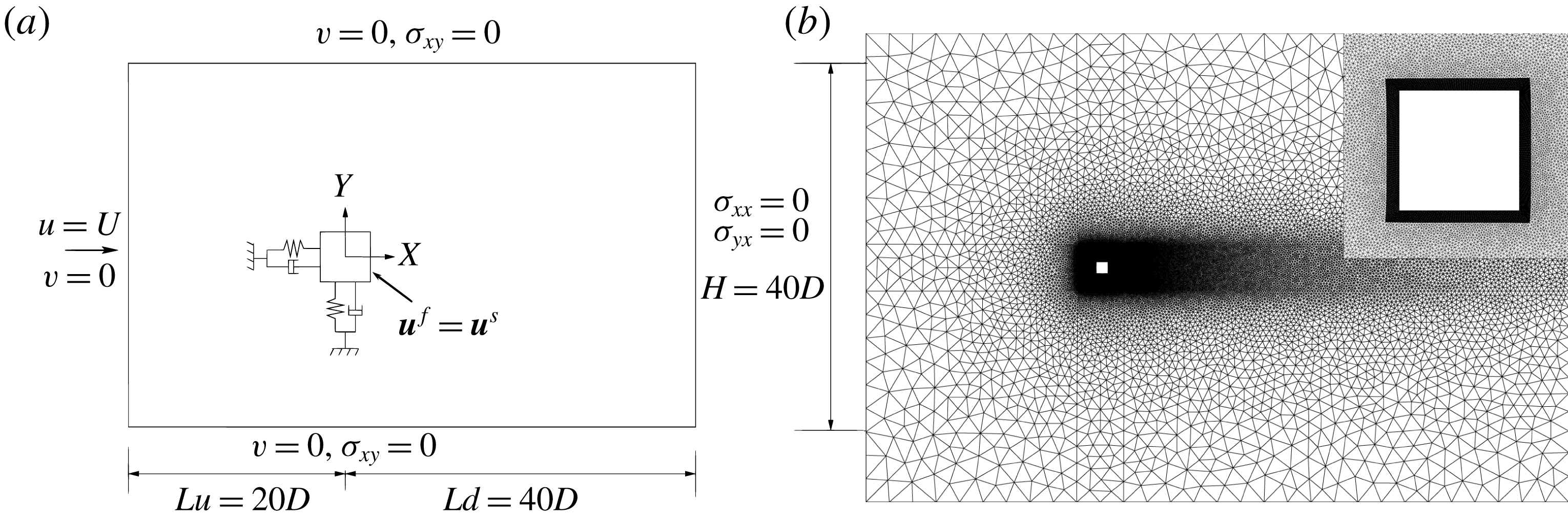
Figure 1. Full-order problem set-up for fluid–structure interaction: (a) schematic diagram of the computational domain and boundary conditions; (b) representative
 $Z$
-plane slice of the unstructured mesh. The top right inset displays the near-cylinder mesh.
$Z$
-plane slice of the unstructured mesh. The top right inset displays the near-cylinder mesh.
3.2 Mesh convergence study
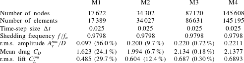
For the high-dimensional approximation of the FOM, the computational domain is discretized using an unstructured finite-element mesh, with a boundary layer mesh surrounding the body and three-node triangle (2-D) and six-node wedge (3-D) elements outside the boundary layer region. Three more grids are generated where the mesh elements are successively increased by approximately a factor of 2, designated as M2, M3 and M4. The discretized domain, along with a close-up view of the corners of the square column, is illustrated in figure 1(b). Grid convergence study results are recorded in table 1 for the lock-in region. All cases for the mesh convergence are simulated at
 $Re=100$
,
$Re=100$
,
 $m^{\ast }=3$
and
$m^{\ast }=3$
and
 $U_{r}=5.0$
. The mesh convergence error is computed by considering the finest mesh M4 as the reference case. The force coefficients, the shedding frequency and the root mean square (r.m.s.) of the transverse amplitude are analysed. It can be seen that values recorded for meshes M3 and M4 differ by less than 1 %. Therefore, mesh M3 is adequate for the present study. Furthermore, the adopted full-order solver and the numerical discretizations have been extensively validated in several earlier studies for both low-
$U_{r}=5.0$
. The mesh convergence error is computed by considering the finest mesh M4 as the reference case. The force coefficients, the shedding frequency and the root mean square (r.m.s.) of the transverse amplitude are analysed. It can be seen that values recorded for meshes M3 and M4 differ by less than 1 %. Therefore, mesh M3 is adequate for the present study. Furthermore, the adopted full-order solver and the numerical discretizations have been extensively validated in several earlier studies for both low-
 $Re$
(Miyanawala, Guan & Jaiman Reference Miyanawala, Guan and Jaiman2016; Jaiman et al.
Reference Jaiman, Guan and Miyanawala2016a
) and moderate-
$Re$
(Miyanawala, Guan & Jaiman Reference Miyanawala, Guan and Jaiman2016; Jaiman et al.
Reference Jaiman, Guan and Miyanawala2016a
) and moderate-
 $Re$
(Jaiman et al.
Reference Jaiman, Guan and Miyanawala2016a
; Miyanawala & Jaiman Reference Miyanawala and Jaiman2018) flows.
$Re$
(Jaiman et al.
Reference Jaiman, Guan and Miyanawala2016a
; Miyanawala & Jaiman Reference Miyanawala and Jaiman2018) flows.
Table 1. Grid convergence study at
 $Re=100$
,
$Re=100$
,
 $m^{\ast }=3$
and
$m^{\ast }=3$
and
 $U_{r}=5.0$
.
$U_{r}=5.0$
.

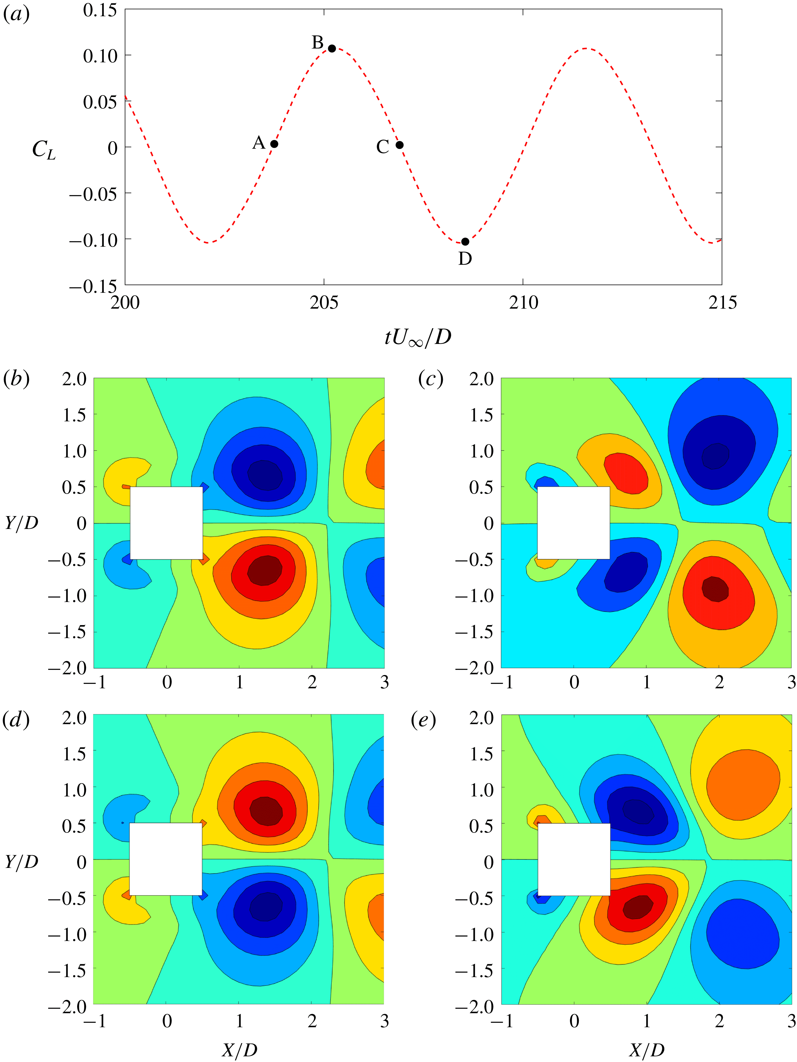
In the next section the modal decomposition of the pressure field is presented for a representative reduced velocity of
 $U_{r}=6.0$
in the lock-in region at
$U_{r}=6.0$
in the lock-in region at
 $(Re,m^{\ast },\unicode[STIX]{x1D701})=(100,3.0,0)$
. The snapshots of the FOM performed for the flow past a vibrating square cylinder are utilized to recover the POD modes and the DEIM points. The accuracy of the linear POD and POD-DEIM is systematically assessed with regard to their effectiveness in extracting the flow features.
$(Re,m^{\ast },\unicode[STIX]{x1D701})=(100,3.0,0)$
. The snapshots of the FOM performed for the flow past a vibrating square cylinder are utilized to recover the POD modes and the DEIM points. The accuracy of the linear POD and POD-DEIM is systematically assessed with regard to their effectiveness in extracting the flow features.
4 Assessment of low-order model for wake decomposition
As described earlier, we incorporate the snapshot POD method described to obtain the low-dimensional decomposition of the wake dynamics. As found in Miyanawala & Jaiman (Reference Miyanawala and Jaiman2018), the laminar bluff body flow involves just a few significant features. It will be ineffective to generate the entire set of POD modes, e.g. 87 120 modes (
 $=$
mesh count) for this particular problem. Hence, we use the snapshot POD technique and obtain just the most significant POD modes, which are a few orders of magnitude smaller. We reconstruct the pressure field using the linear and nonlinear techniques and compare their effectiveness in capturing the organized wake features. In the present analysis the unsteady pressure field values for all the mesh points are collected into an
$=$
mesh count) for this particular problem. Hence, we use the snapshot POD technique and obtain just the most significant POD modes, which are a few orders of magnitude smaller. We reconstruct the pressure field using the linear and nonlinear techniques and compare their effectiveness in capturing the organized wake features. In the present analysis the unsteady pressure field values for all the mesh points are collected into an
 $m\times k$
matrix
$m\times k$
matrix
 $\boldsymbol{P}$
where
$\boldsymbol{P}$
where
 $m$
(mesh count)
$m$
(mesh count)
 $=$
87 120 and
$=$
87 120 and
 $k$
(number of snapshots)
$k$
(number of snapshots)
 $=$
320. The snapshots are sampled every 50 time steps, i.e. at
$=$
320. The snapshots are sampled every 50 time steps, i.e. at
 $1.25D/U_{\infty }$
intervals (sampling frequency
$1.25D/U_{\infty }$
intervals (sampling frequency
 $=0.8U_{\infty }/D$
). Further details about the determination of the sampling frequency and the adequate number of samples are presented in appendix A. The fluctuation matrix
$=0.8U_{\infty }/D$
). Further details about the determination of the sampling frequency and the adequate number of samples are presented in appendix A. The fluctuation matrix
 $\tilde{\boldsymbol{y}}_{m\times k}$
is then generated by subtracting the mean value (
$\tilde{\boldsymbol{y}}_{m\times k}$
is then generated by subtracting the mean value (
 $\overline{\boldsymbol{P}}$
) of each point over the snapshots
$\overline{\boldsymbol{P}}$
) of each point over the snapshots
 $\tilde{\boldsymbol{Y}}=\boldsymbol{P}-\overline{\boldsymbol{P}}$
. The POD modes are extracted using the eigenvalues
$\tilde{\boldsymbol{Y}}=\boldsymbol{P}-\overline{\boldsymbol{P}}$
. The POD modes are extracted using the eigenvalues
 $\unicode[STIX]{x1D726}_{k\times k}=\text{diag}[\unicode[STIX]{x1D706}_{1},\unicode[STIX]{x1D706}_{2},\ldots ,\unicode[STIX]{x1D706}_{k}]$
and eigenvectors
$\unicode[STIX]{x1D726}_{k\times k}=\text{diag}[\unicode[STIX]{x1D706}_{1},\unicode[STIX]{x1D706}_{2},\ldots ,\unicode[STIX]{x1D706}_{k}]$
and eigenvectors
 $\boldsymbol{{\mathcal{W}}}=[\boldsymbol{w}_{1}\boldsymbol{w}_{2}\cdots \boldsymbol{w}_{k}]$
of the covariance matrix
$\boldsymbol{{\mathcal{W}}}=[\boldsymbol{w}_{1}\boldsymbol{w}_{2}\cdots \boldsymbol{w}_{k}]$
of the covariance matrix
 $\tilde{\boldsymbol{Y}}^{\text{T}}\tilde{\boldsymbol{Y}}\in \mathbb{R}^{k\times k}$
given by
$\tilde{\boldsymbol{Y}}^{\text{T}}\tilde{\boldsymbol{Y}}\in \mathbb{R}^{k\times k}$
given by
 $\tilde{\boldsymbol{Y}}^{\text{T}}\tilde{\boldsymbol{Y}}\boldsymbol{{\mathcal{W}}}=\unicode[STIX]{x1D726}\boldsymbol{{\mathcal{W}}}$
. As presented earlier, the POD modes
$\tilde{\boldsymbol{Y}}^{\text{T}}\tilde{\boldsymbol{Y}}\boldsymbol{{\mathcal{W}}}=\unicode[STIX]{x1D726}\boldsymbol{{\mathcal{W}}}$
. As presented earlier, the POD modes
 $\boldsymbol{{\mathcal{V}}}=[\boldsymbol{v}_{1}\boldsymbol{v}_{2}\cdots \boldsymbol{v}_{k}]$
are related to
$\boldsymbol{{\mathcal{V}}}=[\boldsymbol{v}_{1}\boldsymbol{v}_{2}\cdots \boldsymbol{v}_{k}]$
are related to
 $\unicode[STIX]{x1D726}$
and
$\unicode[STIX]{x1D726}$
and
 $\boldsymbol{{\mathcal{W}}}$
by
$\boldsymbol{{\mathcal{W}}}$
by
 $\boldsymbol{{\mathcal{V}}}=\tilde{\boldsymbol{Y}}\boldsymbol{{\mathcal{W}}}\unicode[STIX]{x1D726}^{-1/2}$
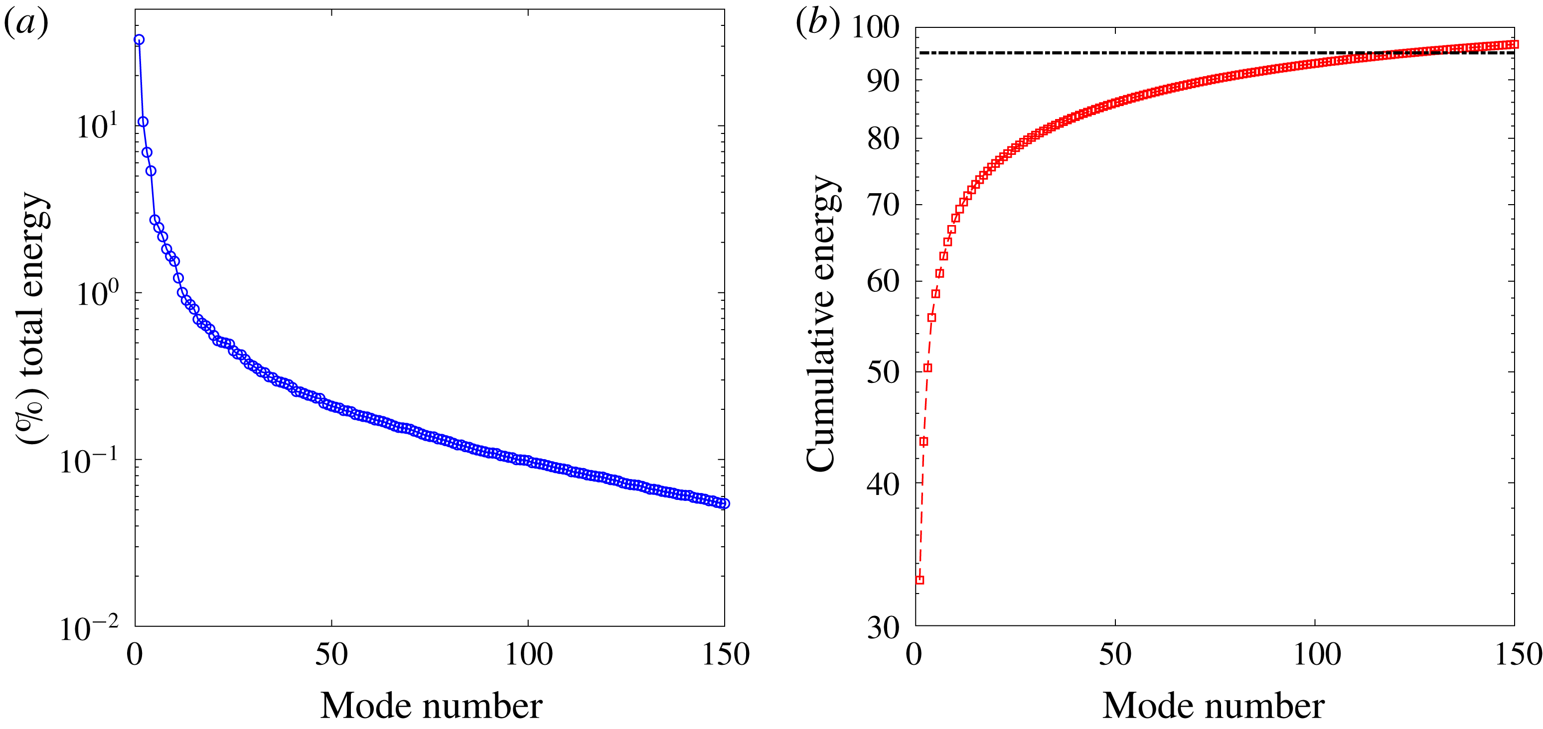
. Each eigenvalue represents the energy/strength of the POD mode. Since the mean pressure distribution is initially removed from the pressure field, the relative strength of the mode directly expresses the contribution from each mode for the pressure fluctuations. Figure 2(a) displays the energy of these modes normalized by the total energy of the 320 modes obtained. It is clear that this energy decays exponentially and the most energetic mode has 56 % of the total energy. In fact, the first nine most significant modes contain 99 % of the total energy of the modes, as shown in figure 2(b). Initially, these nine significant modes are used to recover the pressure field in the linear POD reconstruction. We refer to these modes as mode 1, mode 2, etc. and they are in the descending order of mode energy (
$\boldsymbol{{\mathcal{V}}}=\tilde{\boldsymbol{Y}}\boldsymbol{{\mathcal{W}}}\unicode[STIX]{x1D726}^{-1/2}$
. Each eigenvalue represents the energy/strength of the POD mode. Since the mean pressure distribution is initially removed from the pressure field, the relative strength of the mode directly expresses the contribution from each mode for the pressure fluctuations. Figure 2(a) displays the energy of these modes normalized by the total energy of the 320 modes obtained. It is clear that this energy decays exponentially and the most energetic mode has 56 % of the total energy. In fact, the first nine most significant modes contain 99 % of the total energy of the modes, as shown in figure 2(b). Initially, these nine significant modes are used to recover the pressure field in the linear POD reconstruction. We refer to these modes as mode 1, mode 2, etc. and they are in the descending order of mode energy (
 $\unicode[STIX]{x1D706}_{i}$
). We first incorporate the linear reconstruction method, whereby we assume the final flow field is a linear combination of the flow features captured by the POD modes.
$\unicode[STIX]{x1D706}_{i}$
). We first incorporate the linear reconstruction method, whereby we assume the final flow field is a linear combination of the flow features captured by the POD modes.
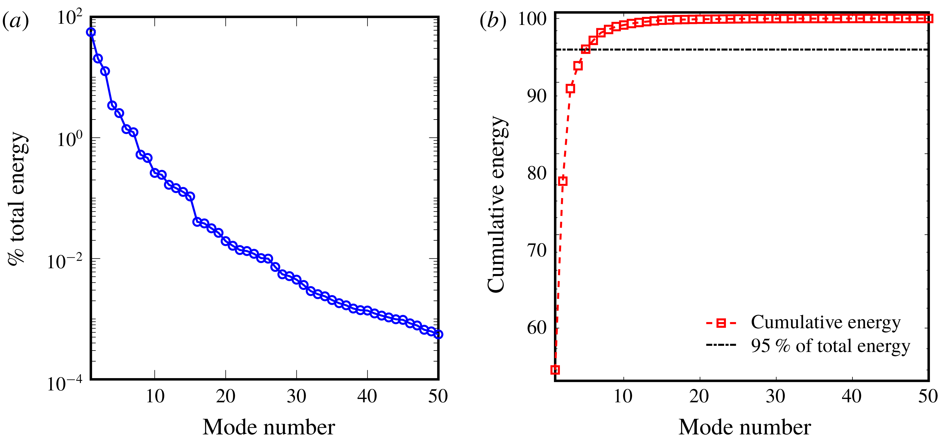
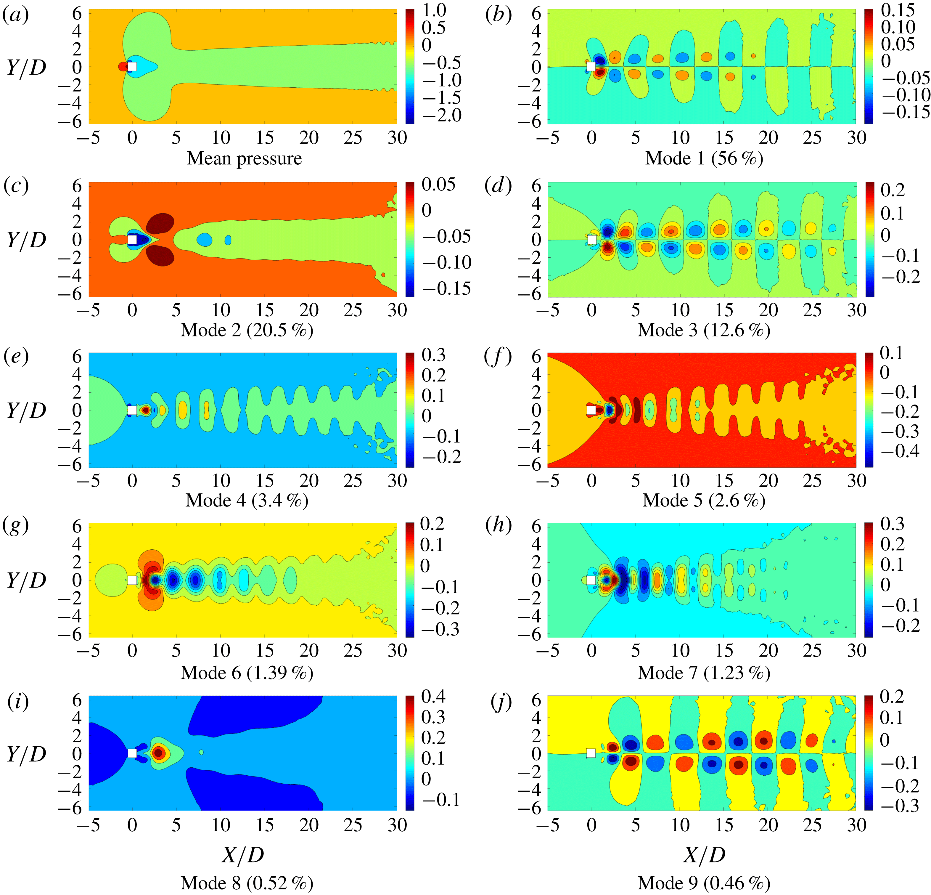
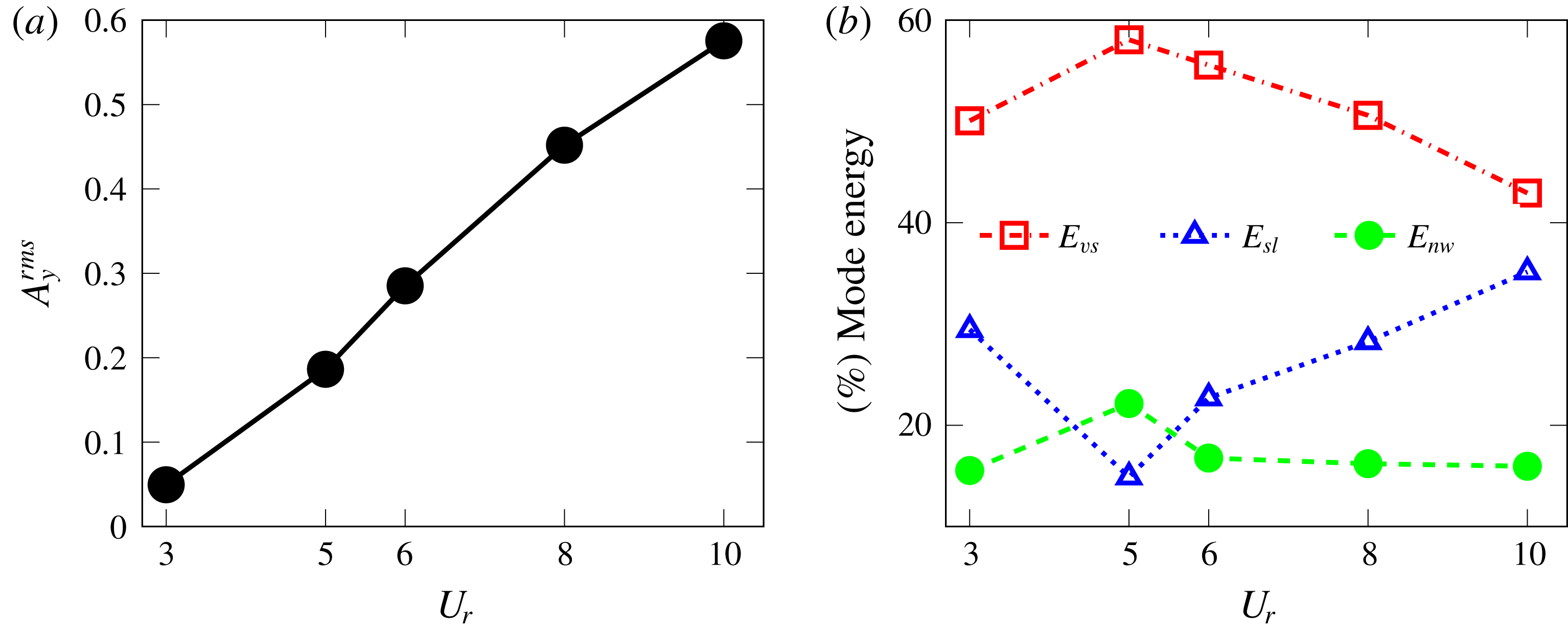
Figure 2. Distribution of modal energy for a laminar flow past a freely vibrating square cylinder: (a) energy decay of POD modes; (b) cumulative energy of POD modes.

Figure 3. The mean field and the first nine significant POD modes. The energy fraction of the POD mode is mentioned in brackets. The values are normalized by
 $1/2\unicode[STIX]{x1D70C}^{f}U_{\infty }^{2}$
. The flow is from left to right.
$1/2\unicode[STIX]{x1D70C}^{f}U_{\infty }^{2}$
. The flow is from left to right.
4.1 Linear POD reconstruction
In the linear POD reconstruction method, the instantaneous pressure field is recovered by the mean and a linear combination of the identified significant modes. In this analysis,
 $r$
is set to
$r$
is set to
 $9$
, which represents the most energetic modes containing
$9$
, which represents the most energetic modes containing
 ${\sim}99\,\%$
of the total contribution to the pressure fluctuations. The temporal coefficients
${\sim}99\,\%$
of the total contribution to the pressure fluctuations. The temporal coefficients
 ${\hat{y}}_{j}$
are determined by the
${\hat{y}}_{j}$
are determined by the
 $L^{2}$
inner product between the fluctuation matrix and the modes as expressed in (2.14). The mean pressure distribution and the first nine POD modes are displayed in figure 3. Note that, throughout this paper, the time-independent fields such as the mean pressure field and POD modes correspond to the initial flow field with zero bluff body motion. (We use a coordinate system fitted to the rigid body: the origin,
$L^{2}$
inner product between the fluctuation matrix and the modes as expressed in (2.14). The mean pressure distribution and the first nine POD modes are displayed in figure 3. Note that, throughout this paper, the time-independent fields such as the mean pressure field and POD modes correspond to the initial flow field with zero bluff body motion. (We use a coordinate system fitted to the rigid body: the origin,
 $(X,Y,Z)=(0,0,0)$
, is always at the centre of the square cylinder.) The mean field is symmetric around the
$(X,Y,Z)=(0,0,0)$
, is always at the centre of the square cylinder.) The mean field is symmetric around the
 $X$
-axis along the wake centreline. This is expected as the time-averaged distribution of the flow past a symmetrical bluff body should be symmetrical. Furthermore, the modes 2, 4, 5, 6, 7 and 8 are symmetric around the wake centreline, while modes 1, 3 and 9 are anti-symmetric with equal values and opposite signs about the wake centreline. As shown in figure 5, the POD time coefficients of these modes have the same frequency as the lift coefficient. It is evident that the first, third and ninth modes correspond predominantly to the Kármán vortex street with alternating positive and negative pressure regions about the
$X$
-axis along the wake centreline. This is expected as the time-averaged distribution of the flow past a symmetrical bluff body should be symmetrical. Furthermore, the modes 2, 4, 5, 6, 7 and 8 are symmetric around the wake centreline, while modes 1, 3 and 9 are anti-symmetric with equal values and opposite signs about the wake centreline. As shown in figure 5, the POD time coefficients of these modes have the same frequency as the lift coefficient. It is evident that the first, third and ninth modes correspond predominantly to the Kármán vortex street with alternating positive and negative pressure regions about the
 $X$
-axis and the pressure contours resulting from a staggered vortex street. By examining figure 5, the time coefficients of the symmetric modes have the same frequency as the drag force. Of these modes, modes 2 and 8 have a high transverse gradient
$X$
-axis and the pressure contours resulting from a staggered vortex street. By examining figure 5, the time coefficients of the symmetric modes have the same frequency as the drag force. Of these modes, modes 2 and 8 have a high transverse gradient
 $(\unicode[STIX]{x2202}/\unicode[STIX]{x2202}y\gg \unicode[STIX]{x2202}/\unicode[STIX]{x2202}x)$
behaviour in the near-wake (
$(\unicode[STIX]{x2202}/\unicode[STIX]{x2202}y\gg \unicode[STIX]{x2202}/\unicode[STIX]{x2202}x)$
behaviour in the near-wake (
 $0.5D$
–
$0.5D$
–
 $5D$
) region almost parallel to the top and bottom edges of the square cylinder, suggesting that these modes represent the influence from the shear layer. Modes 4, 5, 6 and 7 originate from the near-wake region and diffuse symmetrically towards the far wake. These modes have a dominant streamwise gradient
$5D$
) region almost parallel to the top and bottom edges of the square cylinder, suggesting that these modes represent the influence from the shear layer. Modes 4, 5, 6 and 7 originate from the near-wake region and diffuse symmetrically towards the far wake. These modes have a dominant streamwise gradient
 $(\unicode[STIX]{x2202}/\unicode[STIX]{x2202}x\gg \unicode[STIX]{x2202}/\unicode[STIX]{x2202}y)$
compared to the transverse gradient. We can attribute these contributions to the near-wake bubble and its local dynamical property. For ease of explanation, we refer to these modes as the vortex shedding, the shear layer and the near-wake.
$(\unicode[STIX]{x2202}/\unicode[STIX]{x2202}x\gg \unicode[STIX]{x2202}/\unicode[STIX]{x2202}y)$
compared to the transverse gradient. We can attribute these contributions to the near-wake bubble and its local dynamical property. For ease of explanation, we refer to these modes as the vortex shedding, the shear layer and the near-wake.

Figure 4. Absolute value of the time-invariant contribution from each mode to the in-line (
 $|F_{x}^{i}|$
) and cross-flow (
$|F_{x}^{i}|$
) and cross-flow (
 $|F_{y}^{i}|$
) forces. Modes 1, 3 and 9 capture the vortex shedding, modes 2 and 8 correspond to the effect of the shear layer and modes 4, 5, 6 and 7 capture the near-wake bubble effects.
$|F_{y}^{i}|$
) forces. Modes 1, 3 and 9 capture the vortex shedding, modes 2 and 8 correspond to the effect of the shear layer and modes 4, 5, 6 and 7 capture the near-wake bubble effects.
Figure 4 quantifies the time-invariant contributions (
 $F_{j}^{i}$
) from each mode to the drag and lift forces. For the definition of
$F_{j}^{i}$
) from each mode to the drag and lift forces. For the definition of
 $F_{j}^{i}$
,
$F_{j}^{i}$
,
 $j=(x,y)$
is the direction of the force and
$j=(x,y)$
is the direction of the force and
 $i$
is the mode number. These values are calculated based on the fluid–solid boundary values of the mode fields displayed in figure 3. It is clear that the vortex shedding modes (modes 1, 3 and 9) contribute entirely to the lift force, while the shear layer and the near-wake modes contribute entirely to the drag force. Further details of the force decomposition procedure using the modal contributions are presented in appendix B. Due to this directionally independent contribution of the bluff body features for the forces, the time coefficients (
$i$
is the mode number. These values are calculated based on the fluid–solid boundary values of the mode fields displayed in figure 3. It is clear that the vortex shedding modes (modes 1, 3 and 9) contribute entirely to the lift force, while the shear layer and the near-wake modes contribute entirely to the drag force. Further details of the force decomposition procedure using the modal contributions are presented in appendix B. Due to this directionally independent contribution of the bluff body features for the forces, the time coefficients (
 ${\hat{y}}_{j}(t)$
) of these modes should display the same frequencies of the lift and drag forces.
${\hat{y}}_{j}(t)$
) of these modes should display the same frequencies of the lift and drag forces.
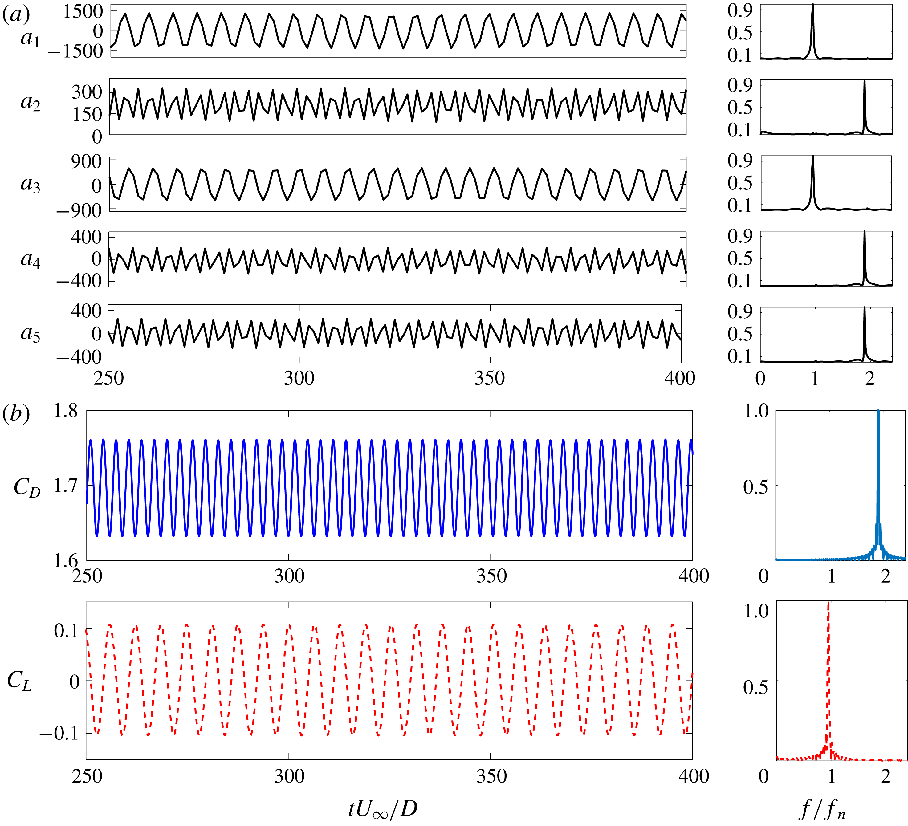
Figure 5. Time history and FFT comparisons: (a) temporal coefficients of first five POD modes; (b) force coefficients. Note that modes 2, 4 and 5 have the same frequency (
 $2f_{n}$
) as the drag and modes 1 and 3 have the same frequency (
$2f_{n}$
) as the drag and modes 1 and 3 have the same frequency (
 $f_{n}$
) as the lift.
$f_{n}$
) as the lift.
The time histories and the fast Fourier transform (FFT) spectra of the first five POD modes are shown in figure 5(a). The first and third mode coefficients have a low-frequency sinusoidal variation with the natural frequency (
 $f_{n}$
). The second, fourth and fifth mode coefficients have a non-zero mean with a frequency
$f_{n}$
). The second, fourth and fifth mode coefficients have a non-zero mean with a frequency
 ${\approx}2f_{n}$
. Interestingly, as presented in figure 5(b),
${\approx}2f_{n}$
. Interestingly, as presented in figure 5(b),
 $f_{n}$
and
$f_{n}$
and
 $2f_{n}$
coincide with the frequencies of lift and drag, respectively. Hence, we can further confirm that modes 1 and 3 make their sole contribution to the fluctuating lift while modes 2, 4 and 5 contribute to the drag force. From these observations, we can further confirm that the vortex shedding process contributes exclusively to the lift force and the near-wake and the shear layer phenomena influence the drag force.
$2f_{n}$
coincide with the frequencies of lift and drag, respectively. Hence, we can further confirm that modes 1 and 3 make their sole contribution to the fluctuating lift while modes 2, 4 and 5 contribute to the drag force. From these observations, we can further confirm that the vortex shedding process contributes exclusively to the lift force and the near-wake and the shear layer phenomena influence the drag force.

Figure 6. Comparison between POD reconstruction and FOM result: pressure distribution obtained by (a) full-order model, (b) linear POD reconstruction, and (c) the relative error (%). Maximum error percentage is less than 2 %. The highly nonlinear near-wake region and the vortex cores have the highest error. The pressure values are normalized by
 $(\unicode[STIX]{x1D70C}^{f}U_{\infty }^{2})/2$
. The flow is from left to right.
$(\unicode[STIX]{x1D70C}^{f}U_{\infty }^{2})/2$
. The flow is from left to right.
Using the POD procedure, we successfully decompose the flow field into physically significant features. We reconstruct the same field combining these modes in the linear POD technique such that utilizing (2.13) for the pressure field gives
 $P(t)\approx \overline{P}+\sum _{j=1}^{r}{\hat{y}}_{j}(t)\boldsymbol{v}_{j}$
. Figure 6 illustrates the pressure distribution at
$P(t)\approx \overline{P}+\sum _{j=1}^{r}{\hat{y}}_{j}(t)\boldsymbol{v}_{j}$
. Figure 6 illustrates the pressure distribution at
 $tU_{\infty }/D=100$
using the linear POD reconstruction. The recovered POD mode is compared with the result obtained from the FOM. A good match with a maximum relative local error of less than
$tU_{\infty }/D=100$
using the linear POD reconstruction. The recovered POD mode is compared with the result obtained from the FOM. A good match with a maximum relative local error of less than
 $2\,\%$
can be seen in figure 6. To quantify the accuracy of the entire flow field recovery, the normalized r.m.s. error of the entire distribution is considered. The r.m.s. error
$2\,\%$
can be seen in figure 6. To quantify the accuracy of the entire flow field recovery, the normalized r.m.s. error of the entire distribution is considered. The r.m.s. error
 $\unicode[STIX]{x1D716}^{rms}$
is given by
$\unicode[STIX]{x1D716}^{rms}$
is given by
 $$\begin{eqnarray}\unicode[STIX]{x1D716}^{rms}=\frac{\displaystyle \sqrt{\sum (P_{FOM}-P_{POD})^{2}/n_{c}}}{|\overline{P_{100}}|}\times 100,\end{eqnarray}$$
where
 $P_{FOM}$
and
$P_{FOM}$
and
 $P_{POD}$
are the pressure values of the mesh nodes extracted from the FOM and the POD reconstruction, respectively,
$P_{POD}$
are the pressure values of the mesh nodes extracted from the FOM and the POD reconstruction, respectively,
 $n_{c}$
is the node count of the mesh and
$n_{c}$
is the node count of the mesh and
 $|\overline{P_{100}}|$
is the mean pressure of the field. When nine modes are used, this error is
$|\overline{P_{100}}|$
is the mean pressure of the field. When nine modes are used, this error is
 $\unicode[STIX]{x1D716}^{rms}=3.78\,\%$
. In this linear reconstruction, the highest error is observed at the regions known to exhibit nonlinear variation, such as the near-wake region, the shear layer and the vortex cores. Next, we analyse the POD-DEIM technique to improve the accuracy in these nonlinear flow features using the snapshot sequence and their respective DEIM points.
$\unicode[STIX]{x1D716}^{rms}=3.78\,\%$
. In this linear reconstruction, the highest error is observed at the regions known to exhibit nonlinear variation, such as the near-wake region, the shear layer and the vortex cores. Next, we analyse the POD-DEIM technique to improve the accuracy in these nonlinear flow features using the snapshot sequence and their respective DEIM points.
4.2 Nonlinear POD-DEIM reconstruction
The linear POD reconstruction has the highest error in the nonlinear regions. To reduce this error, more POD modes should be added to the reconstruction, which makes the POD-based reconstruction very expensive. Instead, when the DEIM technique is used, it reduces the calculation load while properly capturing the nonlinearity of the field variable. The DEIM utilizes two POD bases using the snapshot method, namely a first POD basis
 $\boldsymbol{{\mathcal{V}}}$
from the snapshot sequence, and a second basis
$\boldsymbol{{\mathcal{V}}}$
from the snapshot sequence, and a second basis
 $\boldsymbol{{\mathcal{U}}}$
from the nonlinear snapshots via the DEIM points. However, unlike the linear POD reconstruction, the accuracy does not necessarily improve with the number of DEIM points and the number of POD modes employed. Using many DEIM points results in adding contributions from some non-significant indices. In figure 7(a) it is clearly seen that for 100 DEIM points there are few mesh points lying away from the significant nonlinear region which are taken into the calculation. Further, in table 2 we quantify the number of points in the nonlinear wake region as we increase the number of DEIM points. It is clear that the percentage of points in the critical region decreases as we include more points for the DEIM calculation. Owing to the nonlinear combination of the POD modes, including additional insignificant modes can increase the total error. As shown in figure 7(b), the lowest
$\boldsymbol{{\mathcal{U}}}$
from the nonlinear snapshots via the DEIM points. However, unlike the linear POD reconstruction, the accuracy does not necessarily improve with the number of DEIM points and the number of POD modes employed. Using many DEIM points results in adding contributions from some non-significant indices. In figure 7(a) it is clearly seen that for 100 DEIM points there are few mesh points lying away from the significant nonlinear region which are taken into the calculation. Further, in table 2 we quantify the number of points in the nonlinear wake region as we increase the number of DEIM points. It is clear that the percentage of points in the critical region decreases as we include more points for the DEIM calculation. Owing to the nonlinear combination of the POD modes, including additional insignificant modes can increase the total error. As shown in figure 7(b), the lowest
 $\unicode[STIX]{x1D716}^{rms}=4.05\,\%$
can be obtained when 70 DEIM points are used with seven POD modes. It further establishes that the linear POD reconstruction is generally accurate in a global sense, i.e. the entire flow field reconstruction, in contrast to the nonlinear POD-DEIM. However, figure 8 demonstrates the reconstructed pressure distribution at
$\unicode[STIX]{x1D716}^{rms}=4.05\,\%$
can be obtained when 70 DEIM points are used with seven POD modes. It further establishes that the linear POD reconstruction is generally accurate in a global sense, i.e. the entire flow field reconstruction, in contrast to the nonlinear POD-DEIM. However, figure 8 demonstrates the reconstructed pressure distribution at
 $tU/D=100$
using the optimum number of points and POD modes. There is a significant reduction in the local error as it allows the nonlinear regions to be captured more accurately.
$tU/D=100$
using the optimum number of points and POD modes. There is a significant reduction in the local error as it allows the nonlinear regions to be captured more accurately.

Figure 7. (a) DEIM best points; the top right inset illustrates the near-wake DEIM points. (b) Performance of POD-DEIM compared with linear POD; solid lines denote the linear POD error. The least error is observed when 70 DEIM points are used with seven POD modes.
Table 2. Distribution of DEIM points in the near cylinder wake.
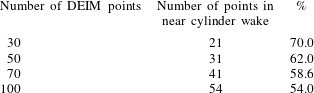
Apart from the global and local accuracy, we further assess the computation time taken by the linear POD and nonlinear POD-DEIM reconstructions. The detailed analysis is presented in appendix C. Theoretically, the DEIM reconstruction process should be
 ${\approx}64$
times faster than linear POD reconstruction and the total DEIM process should be
${\approx}64$
times faster than linear POD reconstruction and the total DEIM process should be
 ${\approx}3.14$
times faster. In the actual computations, when just the reconstructions are considered, the DEIM is
${\approx}3.14$
times faster. In the actual computations, when just the reconstructions are considered, the DEIM is
 $9.28$
times faster than the linear POD. When the total processes are compared, the DEIM has a speed-up of
$9.28$
times faster than the linear POD. When the total processes are compared, the DEIM has a speed-up of
 $3.98$
. In terms of accuracy, the DEIM is more accurate in a local sense since it captures the nonlinearities better than the linear POD reconstruction. However, when the entire fluid domain is considered, the linear POD method is more accurate than the DEIM. It is likely that the DEIM introduces unnecessary nonlinearities to the potential regions, slightly changing the reconstructed field values. When decomposing and reconstructing the laminar flow fields, both linear and nonlinear methods perform to a satisfactory level. Both methods are capable of reaching the required threshold in a reasonable computation time while accurately capturing the flow features of the wake. Henceforth, we employ the POD-DEIM since it has improved accuracy when capturing the nonlinearities in the flow field at a lower computational cost.
$3.98$
. In terms of accuracy, the DEIM is more accurate in a local sense since it captures the nonlinearities better than the linear POD reconstruction. However, when the entire fluid domain is considered, the linear POD method is more accurate than the DEIM. It is likely that the DEIM introduces unnecessary nonlinearities to the potential regions, slightly changing the reconstructed field values. When decomposing and reconstructing the laminar flow fields, both linear and nonlinear methods perform to a satisfactory level. Both methods are capable of reaching the required threshold in a reasonable computation time while accurately capturing the flow features of the wake. Henceforth, we employ the POD-DEIM since it has improved accuracy when capturing the nonlinearities in the flow field at a lower computational cost.
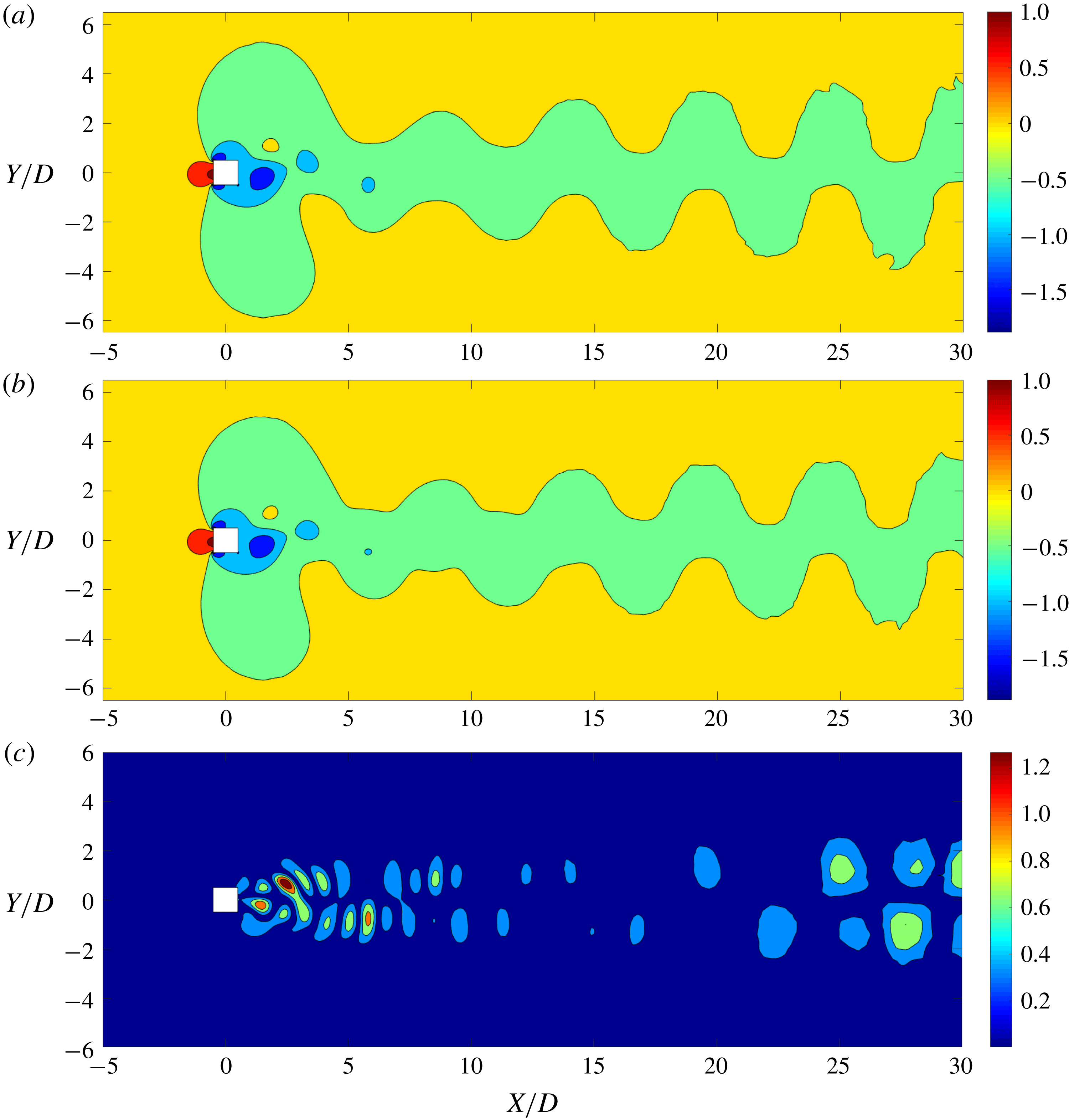
Figure 8. Comparison of POD-DEIM and FOM results: pressure distribution obtained by (a) FOM, (b) POD-DEIM reconstruction, and (c) the relative error of the reconstruction (%). Maximum error percentage is less than 1.5 %. The error in the highly nonlinear regions has reduced compared to the linear POD reconstruction. The pressure values are normalized by
 $1/2\unicode[STIX]{x1D70C}^{f}U_{\infty }^{2}$
. The flow is from left to right.
$1/2\unicode[STIX]{x1D70C}^{f}U_{\infty }^{2}$
. The flow is from left to right.
4.3 Drag and lift modes
In this section we analyse the behaviour of different modes in the near-cylinder region and explain the exclusive nature of their contributions to the pressure-induced drag and lift forces exerted on the oscillating cylinder in a uniform flow. Here, the vortex shedding modes are referred to as the lift modes, while the shear layer and the near wake represent the drag modes. Figure 9 displays the combined variation of the lift modes during a single cycle of lift. Note that the motion of the cylinder is not shown for this reconstruction as the POD modes are time invariant. The lift modes vary in an alternating manner in the four quadrants. The variation is anti-symmetric about the streamwise centreline. In the maximum lift case (point B in figure 9
a), the positive pressure force difference (i.e.
 $+Y$
-direction) in the downstream quadrants dominates the small negative difference in the upstream quadrants, and vice versa for the minimum lift (point D). In the zero-lift cases (points A and C), the upstream and downstream pressure force differences tend to become equally strong and cancel each other out. The lift modes vary in such a way that the force on the top two quadrants is equal in magnitude and opposite in direction to the force on the bottom two quadrants. Due to this force cancellation, the vortex shedding (lift) modes make no contribution to the drag force. Hence, the FFT of the drag force does not contain the corresponding harmonic of the natural frequency (
$+Y$
-direction) in the downstream quadrants dominates the small negative difference in the upstream quadrants, and vice versa for the minimum lift (point D). In the zero-lift cases (points A and C), the upstream and downstream pressure force differences tend to become equally strong and cancel each other out. The lift modes vary in such a way that the force on the top two quadrants is equal in magnitude and opposite in direction to the force on the bottom two quadrants. Due to this force cancellation, the vortex shedding (lift) modes make no contribution to the drag force. Hence, the FFT of the drag force does not contain the corresponding harmonic of the natural frequency (
 $f_{n}$
).
$f_{n}$
).

Figure 9. Reconstruction of the lift modes in the near-cylinder region for
 $U_{r}=6.0$
: (a) lift variation; (b) zero lift (increasing) at
$U_{r}=6.0$
: (a) lift variation; (b) zero lift (increasing) at
 $tU_{\infty }/D=203.75$
; (c) maximum lift at
$tU_{\infty }/D=203.75$
; (c) maximum lift at
 $tU_{\infty }/D=205.25$
; (d) zero lift (decreasing) at
$tU_{\infty }/D=205.25$
; (d) zero lift (decreasing) at
 $tU_{\infty }/D=206.85$
; (e) minimum lift at
$tU_{\infty }/D=206.85$
; (e) minimum lift at
 $tU_{\infty }/D=208.50$
. The pressure values are normalized by
$tU_{\infty }/D=208.50$
. The pressure values are normalized by
 $1/2\unicode[STIX]{x1D70C}^{f}U_{\infty }^{2}$
. The contours levels are from
$1/2\unicode[STIX]{x1D70C}^{f}U_{\infty }^{2}$
. The contours levels are from
 $-0.4$
to
$-0.4$
to
 $0.4$
in increments of
$0.4$
in increments of
 $0.1$
. The flow is from left to right.
$0.1$
. The flow is from left to right.
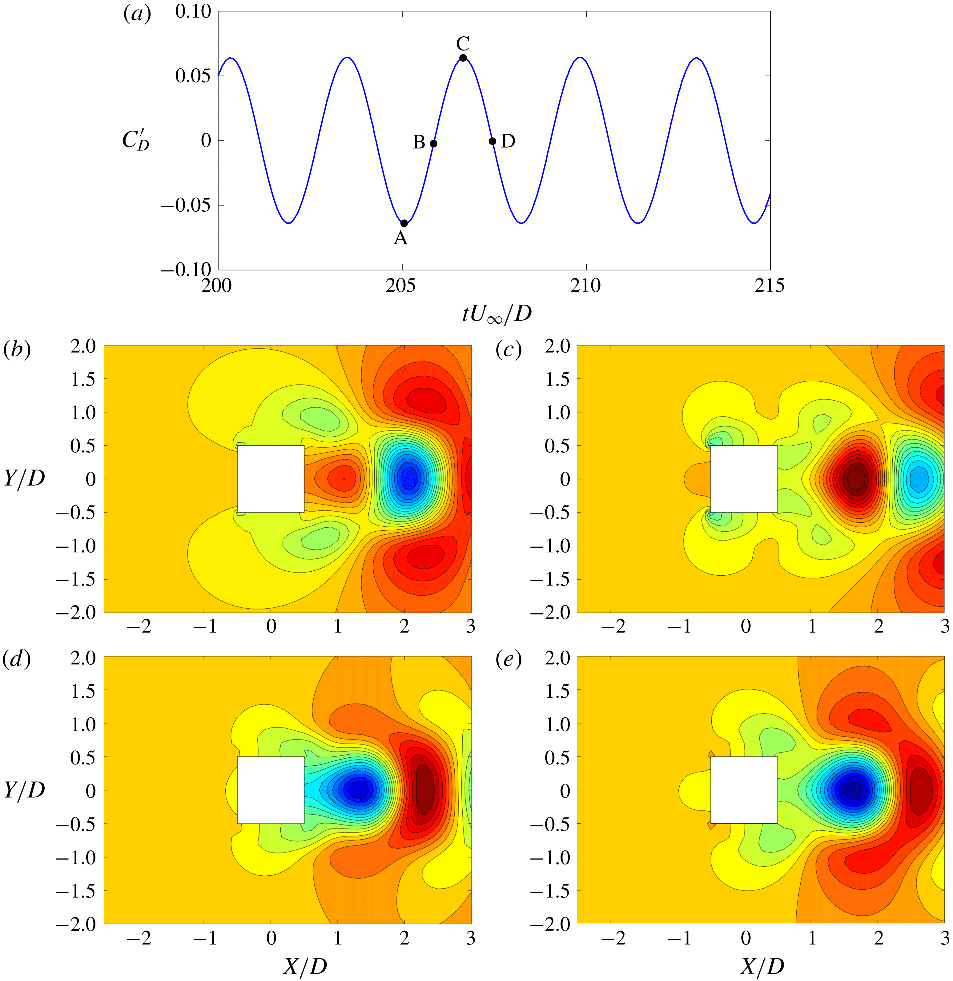
Figure 10. Reconstruction of the drag modes in the near-cylinder region for
 $U_{r}=6.0$
: (a) fluctuation of drag; (b) minimum drag fluctuation at
$U_{r}=6.0$
: (a) fluctuation of drag; (b) minimum drag fluctuation at
 $tU_{\infty }/D=205.05$
; (c) zero drag fluctuation (increasing) at
$tU_{\infty }/D=205.05$
; (c) zero drag fluctuation (increasing) at
 $tU_{\infty }/D=205.85$
; (d) maximum drag fluctuation at
$tU_{\infty }/D=205.85$
; (d) maximum drag fluctuation at
 $tU_{\infty }/D=206.70$
; (e) zero drag fluctuation (decreasing) at
$tU_{\infty }/D=206.70$
; (e) zero drag fluctuation (decreasing) at
 $tU_{\infty }/D=207.40$
. The pressure values are normalized by
$tU_{\infty }/D=207.40$
. The pressure values are normalized by
 $1/2\unicode[STIX]{x1D70C}^{f}U_{\infty }^{2}$
. The contours levels are from
$1/2\unicode[STIX]{x1D70C}^{f}U_{\infty }^{2}$
. The contours levels are from
 $-0.34$
to
$-0.34$
to
 $0.16$
in increments of
$0.16$
in increments of
 $0.025$
. The flow is from left to right.
$0.025$
. The flow is from left to right.
Figure 10 describes the variation of drag modes with the fluctuation of the pressure-induced drag force. The drag fluctuation is defined as
 $C_{Dp}^{\prime }=C_{Dp}(t)-\overline{C_{Dp}}$
. The drag modes vary symmetrically around the wake centreline, hence make no contribution to the lift. Similar to the lift modes, this explains the absence of a
$C_{Dp}^{\prime }=C_{Dp}(t)-\overline{C_{Dp}}$
. The drag modes vary symmetrically around the wake centreline, hence make no contribution to the lift. Similar to the lift modes, this explains the absence of a
 $2f_{n}$
harmonic in the lift. The maximum drag fluctuation (point C) is higher than the minimum drag fluctuation (point A). Further, at the zero drag fluctuation points (B and D), the magnitude of the drag fluctuation remains positive. This further confirms that the drag modes exert a non-zero mean drag on the bluff body, apart from the drag force due to the base flow.
$2f_{n}$
harmonic in the lift. The maximum drag fluctuation (point C) is higher than the minimum drag fluctuation (point A). Further, at the zero drag fluctuation points (B and D), the magnitude of the drag fluctuation remains positive. This further confirms that the drag modes exert a non-zero mean drag on the bluff body, apart from the drag force due to the base flow.
With the aforementioned observations, the decomposition of force due to the pressure field on a moving bluff body based on the contributions from different POD modes can be expressed as
 $$\begin{eqnarray}F_{j}(t)=F_{j}^{0}+\mathop{\sum }_{i=1}^{n_{rj}}b_{j}^{i}(t)F_{j}^{i},\end{eqnarray}$$
where
 $F_{j}$
is the force in a particular direction (
$F_{j}$
is the force in a particular direction (
 $j=x$
for in-line and
$j=x$
for in-line and
 $j=y$
for transverse).
$j=y$
for transverse).
 $F_{j}^{0}$
is the time-independent contribution from the mean field and
$F_{j}^{0}$
is the time-independent contribution from the mean field and
 $F_{j}^{i}$
is the time-independent pressure fluctuation contribution calculated for the
$F_{j}^{i}$
is the time-independent pressure fluctuation contribution calculated for the
 $i$
th mode. While
$i$
th mode. While
 $b_{j}^{i}(t)$
is the time-dependent coefficient of the
$b_{j}^{i}(t)$
is the time-dependent coefficient of the
 $i$
th mode for the force in direction
$i$
th mode for the force in direction
 $j$
,
$j$
,
 $n_{rj}$
is the number of POD modes with a significant contribution to the particular force. Using the snapshot data, we can determine
$n_{rj}$
is the number of POD modes with a significant contribution to the particular force. Using the snapshot data, we can determine
 $b_{j}^{i}(t)$
for the streamwise and transverse forces as
$b_{j}^{i}(t)$
for the streamwise and transverse forces as
 $$\begin{eqnarray}b_{j}^{i}(t)=\frac{F_{j}(t)-F_{j}^{0}}{F_{j}^{i}n_{rj}}.\end{eqnarray}$$
The complete description of this force decomposition and its usage is provided in appendix B.
Table 3. Force contributions from the mean field and POD modes.
 $\overline{b_{j}^{i}}$
denotes the time-averaged force coefficient.
$\overline{b_{j}^{i}}$
denotes the time-averaged force coefficient.
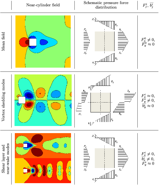
Table 3 summarizes the qualitative analysis of the contributions from the mean field and the modes to the pressure drag and lift forces. The mean field has a symmetric pressure distribution about the wake centreline, hence contributes solely to the time-independent component of the drag force. The vortex shedding modes have an anti-symmetric pressure distribution throughout the time history, hence they make no drag force contribution. We observe that these lift force contributions have a near-zero mean (similar to the lift variation) as well. The shear layer and near-wake modes have the same qualitative properties of the mean field, but their contributions to the drag force are time-dependent. The POD modes provide a deep insight into important flow features and their contribution to the wake dynamics. It is important to investigate their variation with different flow conditions, i.e. the parameters mentioned in (3.1). The variation of POD modes and their contribution to wake dynamics with reduced velocity is examined in the next section, with the aim of explaining the role of the wake features in sustaining the synchronized wake–body motion.
5 Wake feature interaction and sustenance of lock-in
In this section we investigate the relative contributions from different features to the pressure fluctuations and eventually the forces due to the pressure field on the freely oscillating bluff body. When a bluff body is free to oscillate in a current flow it undergoes the lock-in phenomenon: the oscillation amplitude significantly increases when the natural frequency of the bluff body approaches the vortex shedding frequency. In Miyanawala et al. (Reference Miyanawala, Guan and Jaiman2016), the lock-in phenomenon for a square cylinder immersed in a laminar flow at
 $Re=100$
is systematically studied.
$Re=100$
is systematically studied.

Figure 11. Response characteristics and decomposition of wake dynamics for a freely vibrating square cylinder at
 $m^{\ast }=3.0$
,
$m^{\ast }=3.0$
,
 $Re=100$
and
$Re=100$
and
 $\unicode[STIX]{x1D701}=0$
: (a) transverse displacement; (b) drag and lift force variations, mode energy contributions from different flow features; (c) vortex shedding; (d) shear layer; (e) near-wake; (f) total mode energy contributions.
$\unicode[STIX]{x1D701}=0$
: (a) transverse displacement; (b) drag and lift force variations, mode energy contributions from different flow features; (c) vortex shedding; (d) shear layer; (e) near-wake; (f) total mode energy contributions.
 $E_{vs},E_{sl},E_{nw}$
denote the relative mode energy of the wake features as a percentage of the total mode energy. The first nine modes, which contain
$E_{vs},E_{sl},E_{nw}$
denote the relative mode energy of the wake features as a percentage of the total mode energy. The first nine modes, which contain
 $99\,\%$
of the total mode energy, are considered. For all
$99\,\%$
of the total mode energy, are considered. For all
 $U_{r}$
values, modes 1 and 3 correspond to the vortex shedding, while mode 2 corresponds to the shear layer. The flow features of modes 4–9 depend on the
$U_{r}$
values, modes 1 and 3 correspond to the vortex shedding, while mode 2 corresponds to the shear layer. The flow features of modes 4–9 depend on the
 $U_{r}$
value (e.g. mode 4 is a shear layer mode for
$U_{r}$
value (e.g. mode 4 is a shear layer mode for
 $U_{r}=4,8,10,12$
and a near wake mode for
$U_{r}=4,8,10,12$
and a near wake mode for
 $U_{r}=5,6,7$
).
$U_{r}=5,6,7$
).
Figures 11(a) and 11(b) summarize the bluff body dynamics of a freely vibrating square cylinder. The cylinder undergoes wake–body synchronized lock-in in the range
 $U_{r}\in [4.5,7]$
and the peak oscillation occurs at
$U_{r}\in [4.5,7]$
and the peak oscillation occurs at
 $U_{r}=5.0$
. Figures 11(c–f) elucidate the variation of relative contributions from different modes as a function of the reduced velocity (
$U_{r}=5.0$
. Figures 11(c–f) elucidate the variation of relative contributions from different modes as a function of the reduced velocity (
 $U_{r}$
). It is interesting to note that the three most energetic modes correspond to the same flow features throughout the
$U_{r}$
). It is interesting to note that the three most energetic modes correspond to the same flow features throughout the
 $U_{r}$
range, namely, the first and third modes (vortex shedding) and the second mode (shear layer). However, modes 4–10 vary in this regard, where most of these modes correspond to the near-wake phenomena. We quantify the relative energy contribution from each wake feature by summing the mode energy of the corresponding modes, i.e.
$U_{r}$
range, namely, the first and third modes (vortex shedding) and the second mode (shear layer). However, modes 4–10 vary in this regard, where most of these modes correspond to the near-wake phenomena. We quantify the relative energy contribution from each wake feature by summing the mode energy of the corresponding modes, i.e.
 $$\begin{eqnarray}E_{j}=\frac{\displaystyle \mathop{\sum }_{i=1}^{n_{j}}\unicode[STIX]{x1D706}_{i}}{\displaystyle \mathop{\sum }_{i=1}^{k}\unicode[STIX]{x1D706}_{i}},\end{eqnarray}$$
where
 $E_{j}$
is the relative energy contribution from the wake feature (
$E_{j}$
is the relative energy contribution from the wake feature (
 $j=vs$
for the vortex shedding,
$j=vs$
for the vortex shedding,
 $j=sl$
for the shear layer and
$j=sl$
for the shear layer and
 $j=nw$
for the near-wake),
$j=nw$
for the near-wake),
 $n_{j}$
is the number of significant modes corresponding to a particular flow feature and
$n_{j}$
is the number of significant modes corresponding to a particular flow feature and
 $k$
is the total number of modes. As shown in figure 11(c), the total contribution from the vortex shedding increases in the lock-in region. However, the first mode becomes more energetic, while the third mode is relatively less energetic in this region. Figure 11(d) shows that the contribution from the shear layer modes reduces significantly in the lock-in region. All the individual shear layer modes also follow a similar trend. The near-wake modes depicted in figure 11(e) become more energetic in the lock-in region relative to the pre- and post-lock-in regions. Unlike the vortex shedding and shear layer, the primary and secondary near-wake modes have remarkably similar contributions. A summary of the contributions from the 10 most energetic POD modes corresponding to different physical phenomena is shown in figure 11(f). Note that these 10 modes capture
$k$
is the total number of modes. As shown in figure 11(c), the total contribution from the vortex shedding increases in the lock-in region. However, the first mode becomes more energetic, while the third mode is relatively less energetic in this region. Figure 11(d) shows that the contribution from the shear layer modes reduces significantly in the lock-in region. All the individual shear layer modes also follow a similar trend. The near-wake modes depicted in figure 11(e) become more energetic in the lock-in region relative to the pre- and post-lock-in regions. Unlike the vortex shedding and shear layer, the primary and secondary near-wake modes have remarkably similar contributions. A summary of the contributions from the 10 most energetic POD modes corresponding to different physical phenomena is shown in figure 11(f). Note that these 10 modes capture
 ${\approx}99\,\%$
of the total mode energy. It is clear that the shear layer contributions decrease while the vortex shedding and the near-wake contributions increase in the lock-in region. In the post-lock-in region, the relative contributions from the flow features remain almost constant. These observations pose an important question: why are the vortex shedding and near-wake bubble energized and why is the shear layer weakened during the lock-in? In that relation, we propose a cycle to explain this counter-intuitive behaviour of the decomposed wake features.
${\approx}99\,\%$
of the total mode energy. It is clear that the shear layer contributions decrease while the vortex shedding and the near-wake contributions increase in the lock-in region. In the post-lock-in region, the relative contributions from the flow features remain almost constant. These observations pose an important question: why are the vortex shedding and near-wake bubble energized and why is the shear layer weakened during the lock-in? In that relation, we propose a cycle to explain this counter-intuitive behaviour of the decomposed wake features.

Figure 12. (a) Schematic of the interaction between bluff body motion, vortex shedding and shear layer instability in the lock-in region. (b–e) Primary shear layer mode variation for different
 $U_{r}$
regimes. The flow is from left to right. In the lock-in regime, the high-gradient region shrinks in the in-line (
$U_{r}$
regimes. The flow is from left to right. In the lock-in regime, the high-gradient region shrinks in the in-line (
 $X$
) and expands in the transverse (
$X$
) and expands in the transverse (
 $Y$
) direction. (f) Cylinder vibration frequency variation with
$Y$
) direction. (f) Cylinder vibration frequency variation with
 $U_{r}$
. (g) Phase difference (
$U_{r}$
. (g) Phase difference (
 $\unicode[STIX]{x1D719}$
) between the fluid force and bluff body motion. The onset of phase jump from
$\unicode[STIX]{x1D719}$
) between the fluid force and bluff body motion. The onset of phase jump from
 $0^{\circ }$
to
$0^{\circ }$
to
 $180^{\circ }$
coincides with the sign change of the primary shear layer mode (c–d).
$180^{\circ }$
coincides with the sign change of the primary shear layer mode (c–d).
Figure 12(a) elaborates the interaction between the wake features and the bluff body motion. When the vortex shedding synchronizes with the bluff body motion, it causes the bluff body to undergo a relatively high-amplitude motion. This widens the wake and eventually the shear layer, decreasing the velocity gradients. This causes the shear layer to give away vorticity flux to the vortex shedding process, intensifying the vortices and the near-wake bubble. The strengthening of vortices increases the in-phase forces with the motion, i.e. the surrounding fluid flow tends to supply higher energy to the structure. As illustrated in Jauvtis & Williamson (Reference Jauvtis and Williamson2004), the force
 $F_{v}$
and the energy transfer rate
$F_{v}$
and the energy transfer rate
 $\dot{e_{v}}$
due to the principal vortices can be analysed using the following simple analytical relations:
$\dot{e_{v}}$
due to the principal vortices can be analysed using the following simple analytical relations:
 $$\begin{eqnarray}\displaystyle & \displaystyle F_{v}=\unicode[STIX]{x1D70C}^{f}\unicode[STIX]{x1D6E4}U_{v}, & \displaystyle\end{eqnarray}$$
 $$\begin{eqnarray}\displaystyle & \displaystyle \dot{e_{v}}=\unicode[STIX]{x1D70C}^{f}\unicode[STIX]{x1D6E4}U_{v}{\dot{y}}, & \displaystyle\end{eqnarray}$$
where
 $\unicode[STIX]{x1D6E4}$
is the vortex strength,
$\unicode[STIX]{x1D6E4}$
is the vortex strength,
 $U_{v}$
is the streamwise velocity of the predominant vortex relative to the bluff body and
$U_{v}$
is the streamwise velocity of the predominant vortex relative to the bluff body and
 ${\dot{y}}$
is the transverse velocity of the bluff body. It is clear that the increase in the vortex strength will increase the forces and energy transfer to the bluff body. The widening of the high-gradient shear layer region in the lock-in regime can be seen in figures 12(b–e), which demonstrate the primary shear layer mode for the different
${\dot{y}}$
is the transverse velocity of the bluff body. It is clear that the increase in the vortex strength will increase the forces and energy transfer to the bluff body. The widening of the high-gradient shear layer region in the lock-in regime can be seen in figures 12(b–e), which demonstrate the primary shear layer mode for the different
 $U_{r}$
cases. In the pre-lock-in regime, the near-wake region is positive compared to the shear layer region. When
$U_{r}$
cases. In the pre-lock-in regime, the near-wake region is positive compared to the shear layer region. When
 $U_{r}=5.0$
, the maximum amplitude case, it is clear that the high-gradient region has shrunk in the streamwise direction and expanded in the transverse direction. Consequently, the near-wake region and the shear layer region interchange distribution when
$U_{r}=5.0$
, the maximum amplitude case, it is clear that the high-gradient region has shrunk in the streamwise direction and expanded in the transverse direction. Consequently, the near-wake region and the shear layer region interchange distribution when
 $U_{r}=6.0$
, i.e. the near-wake region is negative compared to the shear region. This sign change continues to the post-lock-in regime, where the high-gradient region extends to the streamwise direction and becomes narrower in the transverse direction.
$U_{r}=6.0$
, i.e. the near-wake region is negative compared to the shear region. This sign change continues to the post-lock-in regime, where the high-gradient region extends to the streamwise direction and becomes narrower in the transverse direction.
We further generalize this variation of the wake feature contribution for
 $Re>Re_{cr}$
(
$Re>Re_{cr}$
(
 $=44.7$
(Yao & Jaiman Reference Yao and Jaiman2017)). Figure 13 demonstrates the bluff body motion response and the modal energy contribution from the large-scale features of the wake. The cylinder motion follows a similar trend for
$=44.7$
(Yao & Jaiman Reference Yao and Jaiman2017)). Figure 13 demonstrates the bluff body motion response and the modal energy contribution from the large-scale features of the wake. The cylinder motion follows a similar trend for
 $Re=100,125$
and
$Re=100,125$
and
 $150$
where the lock-in region is detected as
$150$
where the lock-in region is detected as
 $U_{r}\in [4.5,7]$
. This region is slightly shifted to
$U_{r}\in [4.5,7]$
. This region is slightly shifted to
 $U_{r}\in [5.5,8]$
for
$U_{r}\in [5.5,8]$
for
 $Re=70$
. In all cases, we observe a maximum of
$Re=70$
. In all cases, we observe a maximum of
 $A_{y}^{rms}\approx 0.2D$
. Regardless of
$A_{y}^{rms}\approx 0.2D$
. Regardless of
 $Re$
, the wake features exhibit a similar trend in terms of modal energy. As displayed in figures 13(b,d), the vortex shedding and the near-wake modes become more energetic during the lock-in and the shear layer modes become less energetic. This further confirms the proposed interaction cycle for the coupling of the wake features and the bluff body motion.
$Re$
, the wake features exhibit a similar trend in terms of modal energy. As displayed in figures 13(b,d), the vortex shedding and the near-wake modes become more energetic during the lock-in and the shear layer modes become less energetic. This further confirms the proposed interaction cycle for the coupling of the wake features and the bluff body motion.
Using the modal decomposition, we have quantitatively explained the interaction dynamics of the flow features which have been conjectured by many previous studies. For example, many successful VIV suppression techniques are proposed by passive (Law & Jaiman Reference Law and Jaiman2017) and active (Guan et al.
Reference Guan, Narendran, Miyanawala, Ma and Jaiman2017; Narendran et al.
Reference Narendran, Guan, Ma, Choudhary, Hussain and Jaiman2018) methods with the experience-based presumption that preventing the interaction between the shear layer, the vortex street and the near-wake will suppress the synchronized wake–body lock-in phenomena. The cycle proposed above provides a proper physical mechanism for the success of those methods: they prevent the vorticity transfer between the shear layer and the vortex shedding and/or near-wake bubble, which breaks the self-sustenance of the wake interaction cycle. This understanding of the wake features and their interactions will be vital for the development of effective suppression methods and devices for flow-induced vibrations. In this analysis we observe that the synchronization of the wake and bluff body weakens the shear layer and intensifies the vortices and the near-wake bubble. In this
 $Re$
regime there exists a periodic vortex shedding for the stationary and pre-/post-lock-in cases. Hence, it is difficult to state whether the flexibility of the bluff body or the unsteadiness of the fluid flow led to the wake–body synchronization. In what follows, we investigate whether the perturbation of the near-wake bubble via flexibility can sustain the synchronized wake–body interaction at below critical
$Re$
regime there exists a periodic vortex shedding for the stationary and pre-/post-lock-in cases. Hence, it is difficult to state whether the flexibility of the bluff body or the unsteadiness of the fluid flow led to the wake–body synchronization. In what follows, we investigate whether the perturbation of the near-wake bubble via flexibility can sustain the synchronized wake–body interaction at below critical
 $Re$
flow, wherein the well-defined periodic vortex shedding does not exist for the stationary counterpart.
$Re$
flow, wherein the well-defined periodic vortex shedding does not exist for the stationary counterpart.

Figure 13. (a) Transverse amplitude
 $A_{y}^{rms}$
of square cylinder as a function of
$A_{y}^{rms}$
of square cylinder as a function of
 $U_{r}$
for
$U_{r}$
for
 $Re\in [70,150]$
at
$Re\in [70,150]$
at
 $m^{\ast }=3$
and
$m^{\ast }=3$
and
 $\unicode[STIX]{x1D701}=0.0$
and the mode energy contributions from wake features; (b) vortex shedding, (c) shear layer and (d) near-wake bubble at different Reynolds numbers. The vortex shedding and near-wake are energized at the lock-in region while the shear layer mode energy is reduced.
$\unicode[STIX]{x1D701}=0.0$
and the mode energy contributions from wake features; (b) vortex shedding, (c) shear layer and (d) near-wake bubble at different Reynolds numbers. The vortex shedding and near-wake are energized at the lock-in region while the shear layer mode energy is reduced.
6 Synchronized wake–body interaction at below critical Re
At very low Reynolds number, the flow past a bluff body is two-dimensional, steady and symmetric with respect to the wake centreline. The near-wake bubble attached to its surface is the essential feature below the critical Reynolds number
 $Re_{cr}$
, which is formed by the steady separation from the sharp corners of a square cylinder. Two symmetric and counter-rotating recirculation zones are present in the wake bubble. As
$Re_{cr}$
, which is formed by the steady separation from the sharp corners of a square cylinder. Two symmetric and counter-rotating recirculation zones are present in the wake bubble. As
 $Re$
increases above the critical value, a Hopf bifurcation sets in and the flow becomes periodic via the vortex shedding process. For circular and square cylinders, Park & Yang (Reference Park and Yang2016) demonstrated these values to be
$Re$
increases above the critical value, a Hopf bifurcation sets in and the flow becomes periodic via the vortex shedding process. For circular and square cylinders, Park & Yang (Reference Park and Yang2016) demonstrated these values to be
 $Re_{cr}=46.8$
and
$Re_{cr}=46.8$
and
 $44.7$
respectively; this was further confirmed by Yao & Jaiman (Reference Yao and Jaiman2017). Interestingly, when the bluff body is free to vibrate, Meliga & Chomaz (Reference Meliga and Chomaz2011) predicted for a circular cylinder that this unstable boundary will hold when
$44.7$
respectively; this was further confirmed by Yao & Jaiman (Reference Yao and Jaiman2017). Interestingly, when the bluff body is free to vibrate, Meliga & Chomaz (Reference Meliga and Chomaz2011) predicted for a circular cylinder that this unstable boundary will hold when
 $m^{\ast }>1000$
and the Hopf bifurcation will occur at much lower
$m^{\ast }>1000$
and the Hopf bifurcation will occur at much lower
 $Re$
for low
$Re$
for low
 $m^{\ast }$
values. The authors further conjectured that for a circular cylinder there will be a limiting
$m^{\ast }$
values. The authors further conjectured that for a circular cylinder there will be a limiting
 $Re\approxeq 32$
, below which the wake flow will be two-dimensional and steady regardless of the mass ratio
$Re\approxeq 32$
, below which the wake flow will be two-dimensional and steady regardless of the mass ratio
 $m^{\ast }$
.
$m^{\ast }$
.

Figure 14. Response characteristics of wake–body interaction for
 $Re<Re_{cr}$
: dependence of transverse amplitude on
$Re<Re_{cr}$
: dependence of transverse amplitude on
 $U_{r}$
and
$U_{r}$
and
 $Re$
. (a) Reduced velocity range
$Re$
. (a) Reduced velocity range
 $U_{r}\in [4,12]$
for
$U_{r}\in [4,12]$
for
 $Re\in [30,40]$
. (b)
$Re\in [30,40]$
. (b)
 $Re\in [20,40]$
for
$Re\in [20,40]$
for
 $U_{r}=7,8$
. (c) Vibration frequency of the bluff body. (d) The spanwise
$U_{r}=7,8$
. (c) Vibration frequency of the bluff body. (d) The spanwise
 $Z$
-vorticity for a non-synchronized case (
$Z$
-vorticity for a non-synchronized case (
 $U_{r}=4.0,Re=40$
). (e) Unsteady wake in a synchronized case (
$U_{r}=4.0,Re=40$
). (e) Unsteady wake in a synchronized case (
 $U_{r}=7.0,Re=40$
) at
$U_{r}=7.0,Re=40$
) at
 $tU_{\infty }/D=120$
. (f–i) POD modes containing
$tU_{\infty }/D=120$
. (f–i) POD modes containing
 ${\sim}99\,\%$
of the mode energy of the synchronized wake–body case:
${\sim}99\,\%$
of the mode energy of the synchronized wake–body case:
 $U_{r}=7.0,Re=40$
. The flow is from left to right.
$U_{r}=7.0,Re=40$
. The flow is from left to right.
Herein, we observe that for some
 $Re<Re_{cr}$
the spring-mounted square cylinder undergoes significant synchronized wake–body motion for a specific range of
$Re<Re_{cr}$
the spring-mounted square cylinder undergoes significant synchronized wake–body motion for a specific range of
 $U_{r}$
. Figure 14(a) illustrates a variation of high-amplitude motion for
$U_{r}$
. Figure 14(a) illustrates a variation of high-amplitude motion for
 $Re=30,35,40$
. When
$Re=30,35,40$
. When
 $Re$
becomes closer to
$Re$
becomes closer to
 $Re_{cr}$
, the synchronization regime widens and the highest-amplitude
$Re_{cr}$
, the synchronization regime widens and the highest-amplitude
 $U_{r}$
shifts from
$U_{r}$
shifts from
 $U_{r}=8$
to
$U_{r}=8$
to
 $U_{r}=7$
. In contrast to
$U_{r}=7$
. In contrast to
 $Re>Re_{cr}$
cases, we observe no motion of the cylinder in pre- and post-synchronization regimes. We further examine the conjecture of Meliga & Chomaz (Reference Meliga and Chomaz2011) and demonstrate that for a square cylinder this synchronized motion is present when
$Re>Re_{cr}$
cases, we observe no motion of the cylinder in pre- and post-synchronization regimes. We further examine the conjecture of Meliga & Chomaz (Reference Meliga and Chomaz2011) and demonstrate that for a square cylinder this synchronized motion is present when
 $Re\geqslant 26$
(figure 14
b). Additional analysis on these synchronized motion cases revealed that the wake–body system synchronizes to a frequency slightly less than the natural frequency
$Re\geqslant 26$
(figure 14
b). Additional analysis on these synchronized motion cases revealed that the wake–body system synchronizes to a frequency slightly less than the natural frequency
 $f_{n}$
of the bluff body similar to the
$f_{n}$
of the bluff body similar to the
 $Re>Re_{cr}$
lock-in regime (figure 14
c). We observe that, for all synchronized motion cases, the wake is unsteady with some vortex shedding patterns. For example, we can compare the representative
$Re>Re_{cr}$
lock-in regime (figure 14
c). We observe that, for all synchronized motion cases, the wake is unsteady with some vortex shedding patterns. For example, we can compare the representative
 $Z$
-vorticity contours for the zero motion and the synchronized motion cases displayed in figures 14(d) and 14(e), respectively. The zero-motion case is almost identical to the stationary cylinder counterpart, while the synchronized motion case is similar to the lock-in scenario for
$Z$
-vorticity contours for the zero motion and the synchronized motion cases displayed in figures 14(d) and 14(e), respectively. The zero-motion case is almost identical to the stationary cylinder counterpart, while the synchronized motion case is similar to the lock-in scenario for
 $Re>Re_{cr}$
. However, the vortex formation length is very high for this below-
$Re>Re_{cr}$
. However, the vortex formation length is very high for this below-
 $Re_{cr}$
configuration. We further decompose the unsteady wake of the synchronized motion case and examine similar features as
$Re_{cr}$
configuration. We further decompose the unsteady wake of the synchronized motion case and examine similar features as
 $Re>Re_{cr}$
cases, i.e. the vortex shedding (figure 14
f,h), the shear layer (figure 14
g) and the near-wake bubble (figure 14
i).
$Re>Re_{cr}$
cases, i.e. the vortex shedding (figure 14
f,h), the shear layer (figure 14
g) and the near-wake bubble (figure 14
i).
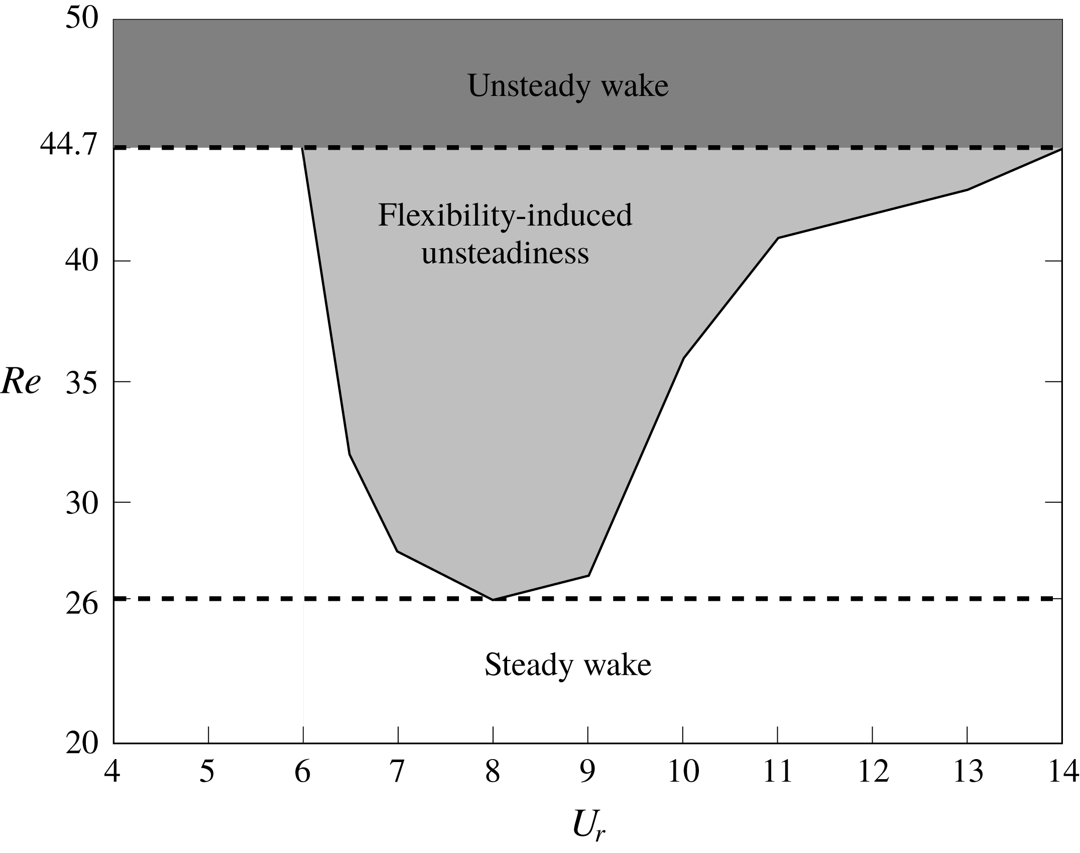
Figure 15. Demarcation of wake unsteadiness for a freely vibrating square cylinder at
 $m^{\ast }=3$
. For the stationary square cylinder, the wake is steady for
$m^{\ast }=3$
. For the stationary square cylinder, the wake is steady for
 $Re<26$
and becomes unsteady for
$Re<26$
and becomes unsteady for
 $Re>44.7$
, as shown by dashed lines.
$Re>44.7$
, as shown by dashed lines.

Figure 16. The energy distribution of the POD modes for
 $Re=22\,000,m^{\ast }=3.0,U_{r}=6.0$
: (a) energy decay of POD modes; (b) cumulative energy of POD modes. The dashed line represents
$Re=22\,000,m^{\ast }=3.0,U_{r}=6.0$
: (a) energy decay of POD modes; (b) cumulative energy of POD modes. The dashed line represents
 $95\,\%$
of the total mode energy.
$95\,\%$
of the total mode energy.
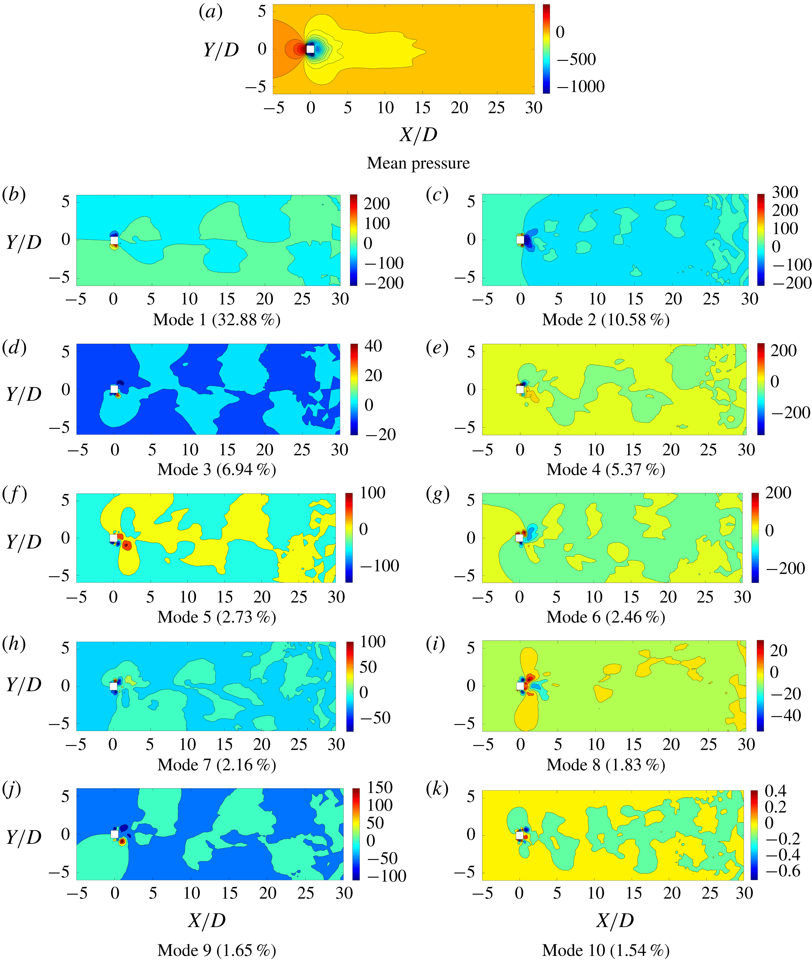
Figure 17. The mean field and the first 10 significant POD modes for an oscillating square cylinder at
 $Re=22\,000$
. The energy fraction of the POD mode is given in brackets. The plots are of the mid
$Re=22\,000$
. The energy fraction of the POD mode is given in brackets. The plots are of the mid
 $Z$
-plane.
$Z$
-plane.
These observations constitute the basic requirement for the wake-bluff body synchronized motion: the bluff body should have an optimal amount of flexibility (i.e. neither too rigid nor too flexible) and the flow needs to have sufficiently large inertia (i.e. higher
 $Re$
) to trigger the unsteadiness in the near-wake bubble. This particular
$Re$
) to trigger the unsteadiness in the near-wake bubble. This particular
 $Re$
is lower than the
$Re$
is lower than the
 $Re_{cr}$
for a fixed bluff body. This means that the flexibility of the solid body provides an avenue for the wake and the spring-mounted body to synchronize, eventually causing the wake to be unsteady. From this numerical experiment, we can deduce that the flexibility of the bluff body is the primary factor driving the synchronized wake–body motion, neither the vortex shedding nor the shear layer roll-up. Hence the most critical wake feature for the onset of wake–body synchronization is the near-wake bubble. When the
$Re_{cr}$
for a fixed bluff body. This means that the flexibility of the solid body provides an avenue for the wake and the spring-mounted body to synchronize, eventually causing the wake to be unsteady. From this numerical experiment, we can deduce that the flexibility of the bluff body is the primary factor driving the synchronized wake–body motion, neither the vortex shedding nor the shear layer roll-up. Hence the most critical wake feature for the onset of wake–body synchronization is the near-wake bubble. When the
 $Re$
is very low (
$Re$
is very low (
 ${<}26$
) this bubble remains steady and the counter-rotating recirculation zones behind the bluff body are stable. For
${<}26$
) this bubble remains steady and the counter-rotating recirculation zones behind the bluff body are stable. For
 $26\leqslant Re\leqslant 44.7$
, it remains same if the bluff body is either too rigid or flexible. However, in this
$26\leqslant Re\leqslant 44.7$
, it remains same if the bluff body is either too rigid or flexible. However, in this
 $Re$
regime, when the bluff body is appropriately flexible, slight perturbations cause distortions in the steady wake. These distortions become periodic and begin to synchronize with the bluff body. This synchronization leads to relatively higher-amplitude oscillations at a frequency slightly less than the natural frequency of the solid body in a vacuum. At the same time, due to the vorticity generation by the unsteadiness developed in the wake, the vortices are shed from the downstream end of the wake bubble.
$Re$
regime, when the bluff body is appropriately flexible, slight perturbations cause distortions in the steady wake. These distortions become periodic and begin to synchronize with the bluff body. This synchronization leads to relatively higher-amplitude oscillations at a frequency slightly less than the natural frequency of the solid body in a vacuum. At the same time, due to the vorticity generation by the unsteadiness developed in the wake, the vortices are shed from the downstream end of the wake bubble.
With the aforementioned findings, we summarize the bluff body wake behaviour for the
 $20\leqslant Re\leqslant 50$
regime in figure 15. We deduce that the root cause of wake–body synchronization is the frequency lock-in between the natural frequency of the bluff body and the near-wake bubble. This further demonstrates that the unsteadiness of the wake can be induced by the flexibility of the bluff body. Moreover, the unsteady wake alone cannot induce high-amplitude bluff body oscillations (e.g. pre- and post-lock-in in
$20\leqslant Re\leqslant 50$
regime in figure 15. We deduce that the root cause of wake–body synchronization is the frequency lock-in between the natural frequency of the bluff body and the near-wake bubble. This further demonstrates that the unsteadiness of the wake can be induced by the flexibility of the bluff body. Moreover, the unsteady wake alone cannot induce high-amplitude bluff body oscillations (e.g. pre- and post-lock-in in
 $Re>Re_{cr}$
). Hence, we can further infer that the wake–body synchronization is induced by the synchronization of the bluff body motion with the near-wake bubble, not with the vortex street. In the next section, we generalize our findings to three-dimensional turbulent flows at moderately high Reynolds number.
$Re>Re_{cr}$
). Hence, we can further infer that the wake–body synchronization is induced by the synchronization of the bluff body motion with the near-wake bubble, not with the vortex street. In the next section, we generalize our findings to three-dimensional turbulent flows at moderately high Reynolds number.
7 Effect of turbulence
In this section we investigate the dynamic decomposition of the wake behind a three-dimensional oscillating square cylinder at
 $Re=22\,000$
, where the wake is fully turbulent. Our aim is to understand the role of turbulence when we extend the wake feature interaction cycle to turbulent flow. To retrieve the high-fidelity data at this
$Re=22\,000$
, where the wake is fully turbulent. Our aim is to understand the role of turbulence when we extend the wake feature interaction cycle to turbulent flow. To retrieve the high-fidelity data at this
 $Re$
, we employ a well-established dynamic subgrid-scale turbulence model in our finite-element formulation. The filtered Navier–Stokes formulation and the determination of the subgrid stress term via the dynamic subgrid-scale model are provided in Jaiman et al. (Reference Jaiman, Guan and Miyanawala2016a
). We incorporate this FOM to generate three-dimensional snapshots of the flow fields, and the POD-Galerkin projection is applied on this high-fidelity data set. At high-
$Re$
, we employ a well-established dynamic subgrid-scale turbulence model in our finite-element formulation. The filtered Navier–Stokes formulation and the determination of the subgrid stress term via the dynamic subgrid-scale model are provided in Jaiman et al. (Reference Jaiman, Guan and Miyanawala2016a
). We incorporate this FOM to generate three-dimensional snapshots of the flow fields, and the POD-Galerkin projection is applied on this high-fidelity data set. At high-
 $Re$
turbulent wake flow, the aforementioned large-scale organized flow features are fragmented into smaller scales until the scales are fine enough to dissipate by the fluid viscosity. Therefore, small-scale modes can have a significant impact on the overall dynamics for the high-
$Re$
turbulent wake flow, the aforementioned large-scale organized flow features are fragmented into smaller scales until the scales are fine enough to dissipate by the fluid viscosity. Therefore, small-scale modes can have a significant impact on the overall dynamics for the high-
 $Re$
turbulent condition, in contrast to the low-
$Re$
turbulent condition, in contrast to the low-
 $Re$
study. Figure 16 demonstrates the mode energy distribution for
$Re$
study. Figure 16 demonstrates the mode energy distribution for
 $Re=22\,000$
. Compared to the low-
$Re=22\,000$
. Compared to the low-
 $Re$
cases, the modal energy is much more distributed among the modes. For instance, the most energetic mode of the
$Re$
cases, the modal energy is much more distributed among the modes. For instance, the most energetic mode of the
 $Re=100$
case contains
$Re=100$
case contains
 $56\,\%$
of the total energy, while it is
$56\,\%$
of the total energy, while it is
 $32.88\,\%$
for the high-
$32.88\,\%$
for the high-
 $Re$
case at
$Re$
case at
 $Re=22\,000$
. Due to this broadening of the mode energy, the energy decay is less steep. For low-
$Re=22\,000$
. Due to this broadening of the mode energy, the energy decay is less steep. For low-
 $Re$
cases, the first five modes contain
$Re$
cases, the first five modes contain
 $95\,\%$
of the total mode energy and the first nine modes contain
$95\,\%$
of the total mode energy and the first nine modes contain
 $99\,\%$
. On the other hand, for the high-
$99\,\%$
. On the other hand, for the high-
 $Re$
case, a total of
$Re$
case, a total of
 $123$
modes are required to capture
$123$
modes are required to capture
 $95\,\%$
of the energy and
$95\,\%$
of the energy and
 $211$
modes are required for
$211$
modes are required for
 $99\,\%$
. We further investigate this distribution of the mode energy with the presumption that the presence of broadband turbulence is the key factor.
$99\,\%$
. We further investigate this distribution of the mode energy with the presumption that the presence of broadband turbulence is the key factor.

Figure 18. Time-dependent contributions of the 10 most energetic modes and their normalized FFT spectra for the
 $Re=22\,000$
case.
$Re=22\,000$
case.
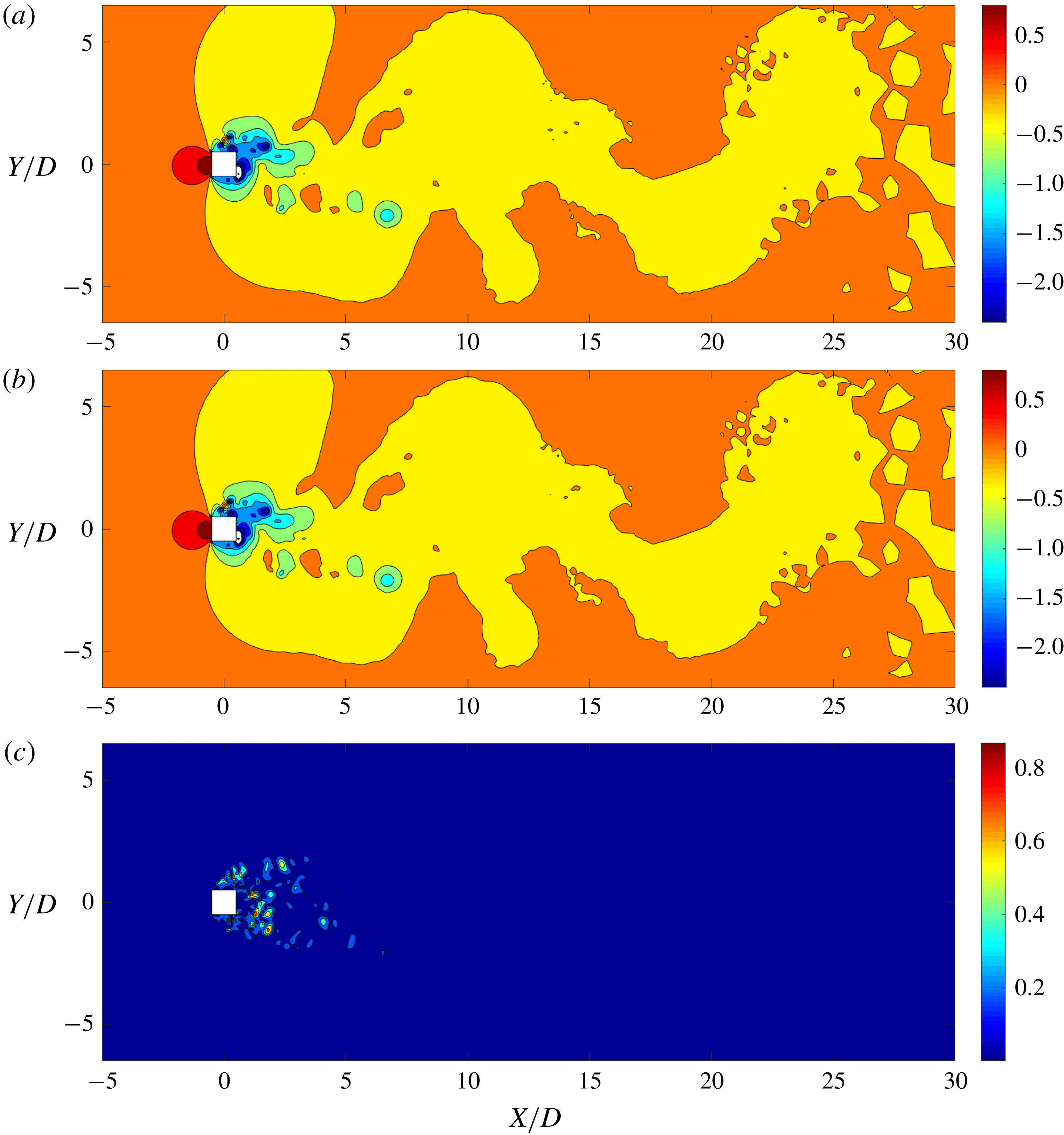
Figure 19. FOM and POD-DEIM reconstructed pressure field comparison for the
 $Re=22\,000$
case at
$Re=22\,000$
case at
 $tU_{\infty }/D=100$
: pressure distribution obtained by (a) FOM and (b) 123 POD modes and 200 DEIM points, and (c) the relative error (%). The plots are of the mid
$tU_{\infty }/D=100$
: pressure distribution obtained by (a) FOM and (b) 123 POD modes and 200 DEIM points, and (c) the relative error (%). The plots are of the mid
 $Z$
-plane. The pressure values are normalized by
$Z$
-plane. The pressure values are normalized by
 $1/2\unicode[STIX]{x1D70C}^{f}U_{\infty }^{2}$
. The flow is from left to right.
$1/2\unicode[STIX]{x1D70C}^{f}U_{\infty }^{2}$
. The flow is from left to right.

Figure 20. Response and energy distribution for a freely vibrating square cylinder at
 $Re=22\,000$
: (a) transverse amplitude as a function of reduced velocity; (b) POD mode energy contribution of wake features. Note that
$Re=22\,000$
: (a) transverse amplitude as a function of reduced velocity; (b) POD mode energy contribution of wake features. Note that
 $U_{r}=3.0$
represents the pre-synchronization regime,
$U_{r}=3.0$
represents the pre-synchronization regime,
 $U_{r}=5.0$
and
$U_{r}=5.0$
and
 $6.0$
the wake–body synchronization regime and
$6.0$
the wake–body synchronization regime and
 $U_{r}=8.0$
and
$U_{r}=8.0$
and
 $10.0$
the galloping regime. For the mode energy analysis, the most energetic modes containing 95 % of the total mode energy are considered.
$10.0$
the galloping regime. For the mode energy analysis, the most energetic modes containing 95 % of the total mode energy are considered.
Figure 17 displays the mean pressure field and 10 most energetic POD modes obtained using the same snapshot technique for the moderate-
 $Re$
case. All the modes exhibit distorted and scattered patterns compared to the low-
$Re$
case. All the modes exhibit distorted and scattered patterns compared to the low-
 $Re$
cases. However, the POD modes further illustrate general large-scale features. For example, modes 1, 3, 4, 5, 6, 7 and 9 exhibit the flow patterns related to vortex shedding, while mode 2 is related to the shear layer and modes 8 and 10 are related to the near-wake phenomena. The distortions occur in each mode throughout the spatial domain due to the broadband and multi-scale effects of turbulence, which are not decomposed by the SVD. Turbulence distributes the modal energy across the modes, so that significantly more modes are required to reconstruct the flow field and the underlying wake dynamics. Hence, the POD-based reconstruction becomes computationally more expensive in turbulent flows due to the broadband and multi-scale character.
$Re$
cases. However, the POD modes further illustrate general large-scale features. For example, modes 1, 3, 4, 5, 6, 7 and 9 exhibit the flow patterns related to vortex shedding, while mode 2 is related to the shear layer and modes 8 and 10 are related to the near-wake phenomena. The distortions occur in each mode throughout the spatial domain due to the broadband and multi-scale effects of turbulence, which are not decomposed by the SVD. Turbulence distributes the modal energy across the modes, so that significantly more modes are required to reconstruct the flow field and the underlying wake dynamics. Hence, the POD-based reconstruction becomes computationally more expensive in turbulent flows due to the broadband and multi-scale character.
Similarly, figure 18 demonstrates the broadband nature of turbulence in the temporal domain. Even with the multi-scale spatial distortions, the first mode of the moderate-
 $Re$
case has a similar temporal contribution to the first mode of the low-
$Re$
case has a similar temporal contribution to the first mode of the low-
 $Re$
case, with a single dominant frequency close to the natural frequency of the system. However, the temporal coefficients of the other modes have multiple harmonics. Some of the modes exhibit predominant frequencies among the broadband FFTs. For example, mode 2 has a dominant
$Re$
case, with a single dominant frequency close to the natural frequency of the system. However, the temporal coefficients of the other modes have multiple harmonics. Some of the modes exhibit predominant frequencies among the broadband FFTs. For example, mode 2 has a dominant
 $2f_{n}$
frequency behaviour, mode 3 has
$2f_{n}$
frequency behaviour, mode 3 has
 $f_{n},2f_{n}$
and
$f_{n},2f_{n}$
and
 $3f_{n}$
harmonics, and mode 4 has
$3f_{n}$
harmonics, and mode 4 has
 $f_{n}$
and
$f_{n}$
and
 $2f_{n}$
harmonics. These multiple harmonics occur due to the bombardment of turbulence on the corresponding flow features of the POD modes.
$2f_{n}$
harmonics. These multiple harmonics occur due to the bombardment of turbulence on the corresponding flow features of the POD modes.
Figure 19 displays the pressure field reconstruction using the POD-DEIM technique. The actual instantaneous field contains some distortions and fine near-wake variations, which are not completely captured by the reconstruction process. However, the general large-scale variations are properly reconstructed with a maximum local error of
 ${\approx}2\,\%$
. The broadband energy distributing nature of turbulence has reduced the contribution of significant POD modes to the wake dynamics. Due to this behaviour, many flow features are not captured when few of the most energetic modes are considered for the reconstruction. Hence, the inclusion of many POD modes is required for an accurate reconstruction which makes the POD reconstruction computationally expensive and time-consuming. However, this can be mitigated by selective reconstruction of a few required time steps instead of the entire time history. Using this to our advantage, we investigate the validity of the wake–body interaction cycle at this moderate
${\approx}2\,\%$
. The broadband energy distributing nature of turbulence has reduced the contribution of significant POD modes to the wake dynamics. Due to this behaviour, many flow features are not captured when few of the most energetic modes are considered for the reconstruction. Hence, the inclusion of many POD modes is required for an accurate reconstruction which makes the POD reconstruction computationally expensive and time-consuming. However, this can be mitigated by selective reconstruction of a few required time steps instead of the entire time history. Using this to our advantage, we investigate the validity of the wake–body interaction cycle at this moderate
 $Re$
value.
$Re$
value.
Figure 20 illustrates the response characteristics and the wake feature contributions for the mode energy at
 $Re=22\,000$
. In contrast to the low-
$Re=22\,000$
. In contrast to the low-
 $Re$
cases, the bluff body undergoes galloping at this Reynolds number. We observe the same wake–body synchronization reported in Miyanawala & Jaiman (Reference Miyanawala and Jaiman2018), i.e. 1 : 1 frequency synchronization of the bluff body motion and force at
$Re$
cases, the bluff body undergoes galloping at this Reynolds number. We observe the same wake–body synchronization reported in Miyanawala & Jaiman (Reference Miyanawala and Jaiman2018), i.e. 1 : 1 frequency synchronization of the bluff body motion and force at
 $U_{r}\in [5,6]$
and 1 : 3 synchronization at
$U_{r}\in [5,6]$
and 1 : 3 synchronization at
 $U_{r}=10.0$
. Our analysis here is focused on the 1 : 1 frequency lock-in where the transverse fluid forcing and the bluff body motion are in synchronization. According to figure 20(b), it is evident that the vortex shedding and near-wake modes become more energetic in the synchronized regime, while the shear layer modes become less energetic. This is the same behaviour observed in the low-
$U_{r}=10.0$
. Our analysis here is focused on the 1 : 1 frequency lock-in where the transverse fluid forcing and the bluff body motion are in synchronization. According to figure 20(b), it is evident that the vortex shedding and near-wake modes become more energetic in the synchronized regime, while the shear layer modes become less energetic. This is the same behaviour observed in the low-
 $Re$
analysis, which proves that the proposed wake–body interaction cycle is valid even in the presence of turbulence.
$Re$
analysis, which proves that the proposed wake–body interaction cycle is valid even in the presence of turbulence.
In summary, the presence of turbulence distorts the spatially symmetric/anti-symmetric nature of POD modes and distributes the mode energy throughout many POD modes. The reconstruction requires many modes and the classification of features is more complex at moderately high
 $Re$
. Despite this complexity, the fundamental wake–body interaction process proposed using low-
$Re$
. Despite this complexity, the fundamental wake–body interaction process proposed using low-
 $Re$
analysis is observed to be valid for three-dimensional turbulent flows. Hence, we can conclude that the proposed wake–body interaction cycle in this study is a general cycle for coupled fluid–structure systems.
$Re$
analysis is observed to be valid for three-dimensional turbulent flows. Hence, we can conclude that the proposed wake–body interaction cycle in this study is a general cycle for coupled fluid–structure systems.
8 Concluding remarks
Despite the prevalence of SVD-based modal reduction techniques, there are very few studies on their application to fluid–structure interaction systems. In this paper, we considered the two-degrees-of-freedom free vibration of a square cylinder under laminar and turbulent flows. We explored the capability of POD decomposition to interpret the most significant wake features and their contributions to the forces on the vibrating body interacting with fluid flow. When the linear and nonlinear POD-DEIM reconstructions are contrasted, we found that the DEIM method is faster and has a higher local accuracy since it captures the nonlinearity of the principle vortices and the near-wake region. For the low-
 $Re$
cases, every POD mode clearly represents one of the large-scale flow features: vortex shedding, shear layer or near-wake bubble. In these cases, we further observed that the nine most energetic modes contain
$Re$
cases, every POD mode clearly represents one of the large-scale flow features: vortex shedding, shear layer or near-wake bubble. In these cases, we further observed that the nine most energetic modes contain
 ${\approx}99\,\%$
of the energy. Further, we identified that the vortex shedding modes solely contribute to the transverse (lift) force while the shear layer and the near-wake modes solely contribute to the drag force. Based on these observations, we proposed a novel force decomposition for the drag and lift forces which is different from the conventional force decomposition based on the added mass and the viscous force contributions.
${\approx}99\,\%$
of the energy. Further, we identified that the vortex shedding modes solely contribute to the transverse (lift) force while the shear layer and the near-wake modes solely contribute to the drag force. Based on these observations, we proposed a novel force decomposition for the drag and lift forces which is different from the conventional force decomposition based on the added mass and the viscous force contributions.
We examined the POD decomposition for a range of
 $U_{r}$
values and we proposed the mechanism of the sustenance of synchronized wake–body lock-in. This further provided the explanation to the observation that in the lock-in region, even though the kinetic energy is transferred from the fluid to the bluff body, the principle vortices are much more energetic than the pre- and post-lock-in regimes. It is seen that the bluff body motion widens the wake and causes a vorticity transfer from the shear layer to the near-wake and vortices. We proposed the wake feature interaction cycle based on these observations. We further confirmed that this mechanism is valid for the laminar
$U_{r}$
values and we proposed the mechanism of the sustenance of synchronized wake–body lock-in. This further provided the explanation to the observation that in the lock-in region, even though the kinetic energy is transferred from the fluid to the bluff body, the principle vortices are much more energetic than the pre- and post-lock-in regimes. It is seen that the bluff body motion widens the wake and causes a vorticity transfer from the shear layer to the near-wake and vortices. We proposed the wake feature interaction cycle based on these observations. We further confirmed that this mechanism is valid for the laminar
 $Re>Re_{cr}$
range. For below-critical-
$Re>Re_{cr}$
range. For below-critical-
 $Re$
flows, we observed that the bluff body and the wake still synchronize and undergo large-amplitude motion at some
$Re$
flows, we observed that the bluff body and the wake still synchronize and undergo large-amplitude motion at some
 $U_{r}$
values when
$U_{r}$
values when
 $Re\geqslant 26$
. Decomposition of these wakes further exhibited behaviour similar to the synchronized large-amplitude motion cases at
$Re\geqslant 26$
. Decomposition of these wakes further exhibited behaviour similar to the synchronized large-amplitude motion cases at
 $Re>Re_{cr}$
. This revealed that the flexibility of the bluff body induced the unsteadiness in the near-wake bubble, causing it to break and generate the vortices. With this observation, we can conclude that the fundamental requirements for the wake–body synchronized motion are large enough flow inertia and appropriate flexibility of the structure.
$Re>Re_{cr}$
. This revealed that the flexibility of the bluff body induced the unsteadiness in the near-wake bubble, causing it to break and generate the vortices. With this observation, we can conclude that the fundamental requirements for the wake–body synchronized motion are large enough flow inertia and appropriate flexibility of the structure.
When the moderate-
 $Re$
turbulent bluff body flow is decomposed, we observe that all the dominant wake modes are bombarded with different scales of turbulence. The broadband nature of turbulence resulted in a wide mode energy distribution, which required up to 123 modes to reach the
$Re$
turbulent bluff body flow is decomposed, we observe that all the dominant wake modes are bombarded with different scales of turbulence. The broadband nature of turbulence resulted in a wide mode energy distribution, which required up to 123 modes to reach the
 $95\,\%$
mode energy threshold. Further analysis of the time coefficients of the modes confirmed that the large-scale features are battered by the multiple frequency turbulence. However, they generally correspond to a large-scale wake feature similar to the laminar cases. The wake decomposition of turbulent flows for
$95\,\%$
mode energy threshold. Further analysis of the time coefficients of the modes confirmed that the large-scale features are battered by the multiple frequency turbulence. However, they generally correspond to a large-scale wake feature similar to the laminar cases. The wake decomposition of turbulent flows for
 $U_{r}\in [3,10]$
confirmed that the wake interaction cycle proposed for laminar cases is valid for turbulent flows as well.
$U_{r}\in [3,10]$
confirmed that the wake interaction cycle proposed for laminar cases is valid for turbulent flows as well.
Acknowledgements
The first author gratefully acknowledges the financial support from the Ministry of Education, Singapore through the National University of Singapore Research Scholarship. The high-fidelity data sets were obtained using the computational resources at High-Performance Computing (HPC) at the National University of Singapore Computer Center and the National Supercomputing Center (NSCC), Singapore.
Appendix A. Selection of POD modes and sampling frequency
In this appendix we briefly present the process followed to determine the number of POD samples and their sampling frequency. The full-order simulation is run at
 $\unicode[STIX]{x0394}t=0.025D/U_{\infty }$
time steps, i.e. at a frequency
$\unicode[STIX]{x0394}t=0.025D/U_{\infty }$
time steps, i.e. at a frequency
 $f_{FOM}=40U_{\infty }/D$
for 28 000 time-steps which contains
$f_{FOM}=40U_{\infty }/D$
for 28 000 time-steps which contains
 ${\sim}112$
vortex shedding cycles. For reference purposes, we utilize the POD decomposition statistics obtained from 2800 samples at frequency
${\sim}112$
vortex shedding cycles. For reference purposes, we utilize the POD decomposition statistics obtained from 2800 samples at frequency
 $f_{ref}=4U_{\infty }/D$
. For example, the natural frequency is
$f_{ref}=4U_{\infty }/D$
. For example, the natural frequency is
 $f_{n}=0.167U_{\infty }/D$
for the case with
$f_{n}=0.167U_{\infty }/D$
for the case with
 $U_{r}=6.0$
and the POD decomposition can capture up to the
$U_{r}=6.0$
and the POD decomposition can capture up to the
 ${\sim}12$
th harmonic according to the Nyquist criterion. To establish an adequate number of POD modes and the sampling frequency, we carry out a convergence study to minimize computational resources.
${\sim}12$
th harmonic according to the Nyquist criterion. To establish an adequate number of POD modes and the sampling frequency, we carry out a convergence study to minimize computational resources.
Figure 21 illustrates the error of mode energy of the three most energetic modes in comparison with the reference sampling. We select combinations of sampling frequency and number of samples with an error threshold at most 0.5 % for all three modes. Table 4 describes these selected combinations. Out of these 10 selections, we rank all selections which can capture harmonics greater than
 $2f_{n}$
, i.e. sampling frequency at least
$2f_{n}$
, i.e. sampling frequency at least
 $4U_{\infty }/D$
, based on the average error of the three mode energies. We ascertain that the combination of 320 flow field samples with the sampling frequency of
$4U_{\infty }/D$
, based on the average error of the three mode energies. We ascertain that the combination of 320 flow field samples with the sampling frequency of
 $4.8U_{\infty }/D$
(selection no. 5 of table 4) has the lowest average error of the thre modes.
$4.8U_{\infty }/D$
(selection no. 5 of table 4) has the lowest average error of the thre modes.
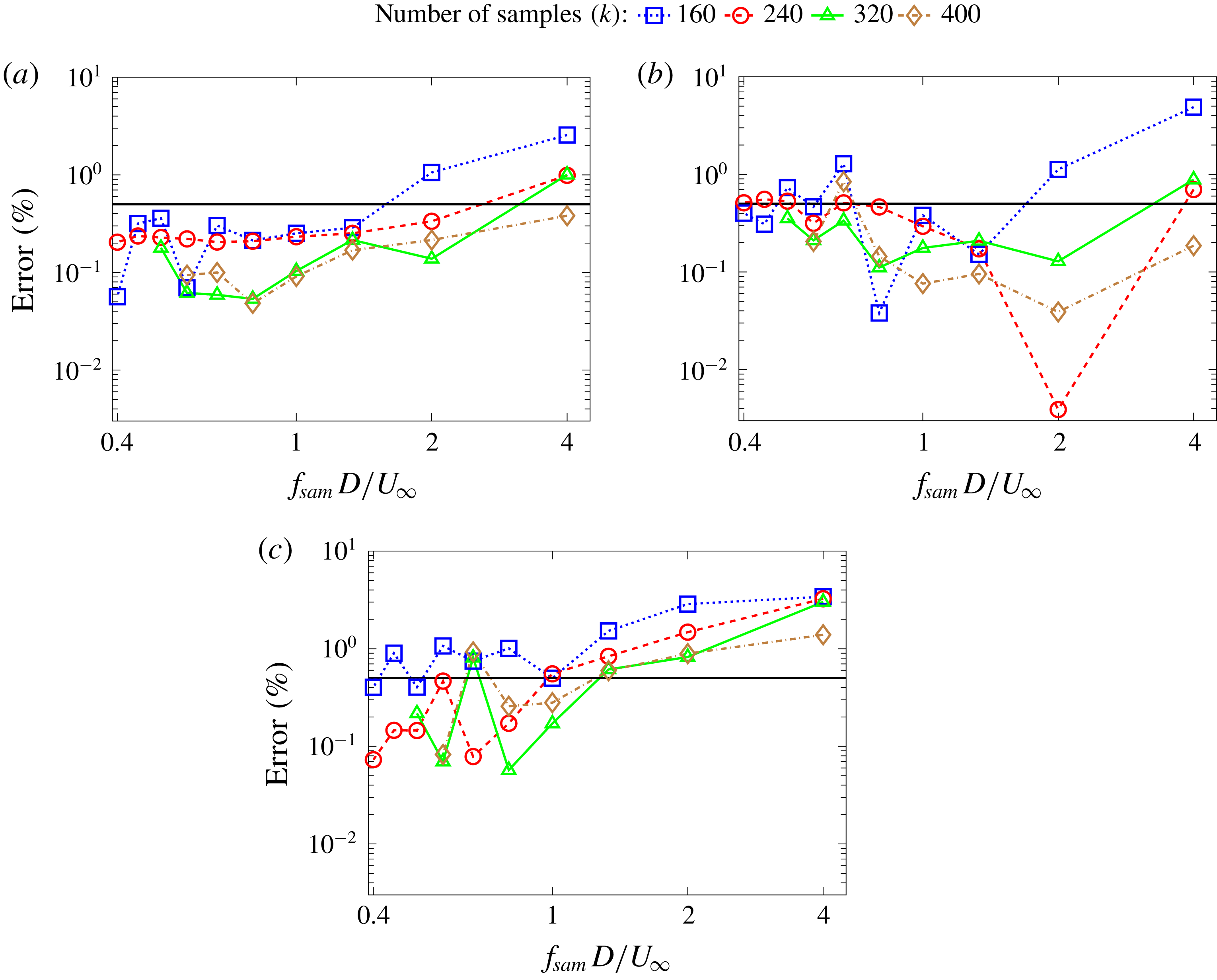
Figure 21. Error trends of mode energy contribution (
 $\unicode[STIX]{x1D706}_{i}/\sum _{j=1}^{k}\unicode[STIX]{x1D706}_{j}$
) from mode
$\unicode[STIX]{x1D706}_{i}/\sum _{j=1}^{k}\unicode[STIX]{x1D706}_{j}$
) from mode
 $i=$
(a) 1, (b) 2 and (c) 3. Here
$i=$
(a) 1, (b) 2 and (c) 3. Here
 $f_{sam}$
is the sampling frequency, and the errors are calculated relative to the reference case with
$f_{sam}$
is the sampling frequency, and the errors are calculated relative to the reference case with
 $f_{sam}D/U_{\infty }=4$
and
$f_{sam}D/U_{\infty }=4$
and
 $k=2800$
. The solid horizontal lines represent the error threshold of 0.5 %.
$k=2800$
. The solid horizontal lines represent the error threshold of 0.5 %.
Table 4. Selected cases based on the convergence study in figure 21. All these cases have relative error at most
 $0.5\,\%$
for the three most significant modes. Cases which are unable to capture at least
$0.5\,\%$
for the three most significant modes. Cases which are unable to capture at least
 $2f_{n}$
harmonic are discarded. The remaining combinations are ranked according to the average error from the three modes.
$2f_{n}$
harmonic are discarded. The remaining combinations are ranked according to the average error from the three modes.
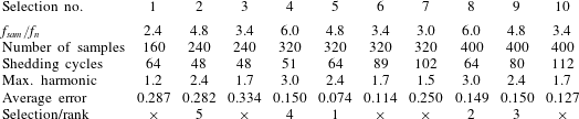
Appendix B. Force decomposition based on modal contribution
The aim of this appendix is to present a general decomposition of the force due to the pressure field exerted on a moving body in an incompressible viscous flow. To begin, we provide some background on existing force decomposition techniques that characterize the fluid inertial and the viscous forces on a moving body. In a pioneering work, Morison, Johnson & Schaaf (Reference Morison, Johnson and Schaaf1950) proposed a force decomposition for the in-line force acting on a cylindrical object which is widely used in many engineering applications. This semi-empirical decomposition can be written as a linear sum of a velocity-squared-dependent drag force and an acceleration-dependent inertial force:
 $$\begin{eqnarray}F(t)=\frac{1}{2}C_{d}D|U|U+\unicode[STIX]{x1D70C}C_{m}\frac{\unicode[STIX]{x03C0}D^{2}}{4}\frac{\text{d}U}{\text{d}t},\end{eqnarray}$$
where
 $C_{d}$
and
$C_{d}$
and
 $C_{m}$
represent the averaged drag and inertia coefficients, which can be determined by experiments or numerical computations. Owing to the nonlinear dependency of these coefficients on the evolution of vorticity field, Sarpkaya (Reference Sarpkaya2001) argued that it ‘does not perform uniformly well in all ranges of
$C_{m}$
represent the averaged drag and inertia coefficients, which can be determined by experiments or numerical computations. Owing to the nonlinear dependency of these coefficients on the evolution of vorticity field, Sarpkaya (Reference Sarpkaya2001) argued that it ‘does not perform uniformly well in all ranges of
 $K$
,
$K$
,
 $\unicode[STIX]{x1D6FD}$
and
$\unicode[STIX]{x1D6FD}$
and
 $k/D$
’, where
$k/D$
’, where
 $K$
denotes the Keulegan–Carpenter number,
$K$
denotes the Keulegan–Carpenter number,
 $\unicode[STIX]{x1D6FD}=Re/K$
and
$\unicode[STIX]{x1D6FD}=Re/K$
and
 $k/D$
is the relative roughness. In Lighthill (Reference Lighthill1986), a different approach is taken by the assertion that the viscous drag and the inviscid inertia force operate independently, by rewriting (B 1):
$k/D$
is the relative roughness. In Lighthill (Reference Lighthill1986), a different approach is taken by the assertion that the viscous drag and the inviscid inertia force operate independently, by rewriting (B 1):
 $$\begin{eqnarray}F(t)=\frac{1}{2}C_{d}\unicode[STIX]{x1D70C}A_{p}U^{2}+C_{m}^{\ast }\unicode[STIX]{x1D70C}\frac{\text{d}U}{\text{d}t}V_{b}.\end{eqnarray}$$
For a flow defined by
 $U(t)=-U_{m}\cos \unicode[STIX]{x1D714}t$
we obtain
$U(t)=-U_{m}\cos \unicode[STIX]{x1D714}t$
we obtain
 $$\begin{eqnarray}C_{F}=-C_{d}|\text{cos}\unicode[STIX]{x1D714}t|\cos \unicode[STIX]{x1D714}t+C_{m}^{\ast }\frac{\unicode[STIX]{x03C0}^{2}}{K}\sin \unicode[STIX]{x1D714}t,\end{eqnarray}$$
where
 $A_{p}$
and
$A_{p}$
and
 $V_{b}$
denote the projected area and the volume of the body, respectively, and
$V_{b}$
denote the projected area and the volume of the body, respectively, and
 $C_{m}^{\ast }$
is the ideal value of the inertia coefficient. However, many studies demonstrate that it is difficult to represent the actual force with this relation as long as a constant value
$C_{m}^{\ast }$
is the ideal value of the inertia coefficient. However, many studies demonstrate that it is difficult to represent the actual force with this relation as long as a constant value
 $C_{m}^{\ast }$
is considered. In particular, Sarpkaya (Reference Sarpkaya2001) clearly demonstrated that the viscous drag force and the inviscid inertia force are not completely independent and it is impossible to decompose the unsteady drag force into an inviscid and a vorticity-drag component. The decomposition of the total force into inviscid and viscous components by Lighthill’s relation (B 2) can be considered as an effort to lump the effects of the complex generation and evolution of the vorticity field into mutually independent forces related to the inviscid inertia and the viscous effects. In such force decomposition techniques, the characteristic vorticity patterns and their dynamics generated during the motion of a body are not included.
$C_{m}^{\ast }$
is considered. In particular, Sarpkaya (Reference Sarpkaya2001) clearly demonstrated that the viscous drag force and the inviscid inertia force are not completely independent and it is impossible to decompose the unsteady drag force into an inviscid and a vorticity-drag component. The decomposition of the total force into inviscid and viscous components by Lighthill’s relation (B 2) can be considered as an effort to lump the effects of the complex generation and evolution of the vorticity field into mutually independent forces related to the inviscid inertia and the viscous effects. In such force decomposition techniques, the characteristic vorticity patterns and their dynamics generated during the motion of a body are not included.

Figure 22. Time-dependent coefficients of pressure force contributions from (a) drag and (b) lift modes.
In what follows, we propose an alternative force decomposition for the in-line (drag) and transverse (lift) pressure forces applied to a bluff body which extends the above decompositions to incorporate significant features of unsteady separated flow. In particular, the unsteady force is decomposed to include the nonlinear generation and evolution of the vorticity field around a moving body in a fluid flow. This decomposition is based on the contributions from different POD modes to the forces and can be written as
 $$\begin{eqnarray}F_{j}(t)=F_{j}^{0}+\mathop{\sum }_{i=1}^{n_{rj}}b_{j}^{i}(t)F_{j}^{i},\end{eqnarray}$$
where
 $F_{j}$
is the force on a particular direction (
$F_{j}$
is the force on a particular direction (
 $j=x$
for the in-line and
$j=x$
for the in-line and
 $j=y$
for transverse). While
$j=y$
for transverse). While
 $F_{j}^{0}$
is the time-independent contribution from the mean field,
$F_{j}^{0}$
is the time-independent contribution from the mean field,
 $F_{j}^{i}$
is the unsteady pressure fluctuation contribution associated with
$F_{j}^{i}$
is the unsteady pressure fluctuation contribution associated with
 $i$
th mode. Here,
$i$
th mode. Here,
 $b_{j}^{i}(t)$
is the time-dependent coefficient of the
$b_{j}^{i}(t)$
is the time-dependent coefficient of the
 $i$
th mode for the force in direction
$i$
th mode for the force in direction
 $j$
and
$j$
and
 $n_{rj}$
is the number of POD modes with a significant contribution for the particular force. Using the snapshot data, we can exactly determine
$n_{rj}$
is the number of POD modes with a significant contribution for the particular force. Using the snapshot data, we can exactly determine
 $b_{j}^{i}(t)$
for the in-line and transverse forces by the relation
$b_{j}^{i}(t)$
for the in-line and transverse forces by the relation
 $$\begin{eqnarray}b_{j}^{i}(t)=\frac{F_{j}(t)-F_{j}^{0}}{F_{j}^{i}n_{rj}}.\end{eqnarray}$$
The magnitude of the modes, the time coefficients and the force contributions introduced in this decomposition fluctuate slightly when flow parameters and the bluff body geometry are changed. Similar to the above methods, we can create databases of
 $F_{j}^{i}$
for different bluff bodies. These databases can then be used to determine the total forces as well as the contribution from each flow feature to the bluff body dynamics. To further generalize the force decomposition, deep learning techniques (Miyanawala & Jaiman Reference Miyanawala and Jaiman2017) for parametric predictions can be employed.
$F_{j}^{i}$
for different bluff bodies. These databases can then be used to determine the total forces as well as the contribution from each flow feature to the bluff body dynamics. To further generalize the force decomposition, deep learning techniques (Miyanawala & Jaiman Reference Miyanawala and Jaiman2017) for parametric predictions can be employed.
Figure 22 presents the reconstructed values of the time dependent coefficients for drag and lift modes. Note that the relevant six out of the first nine modes are considered for the drag and the rest for the lift (i.e.
 $n_{rx}=6$
and
$n_{rx}=6$
and
 $n_{ry}=3$
). In a nutshell, the force component represented by the modal decomposition implicitly characterizes the three constituent components involving an inviscid inertial force, the dynamics of the vorticity field, and a skin friction force.
$n_{ry}=3$
). In a nutshell, the force component represented by the modal decomposition implicitly characterizes the three constituent components involving an inviscid inertial force, the dynamics of the vorticity field, and a skin friction force.
Table 5. Number of FLOPs required for linear and nonlinear POD reconstruction. Mesh count (
 $m$
)
$m$
)
 $=$
87 120, number of snapshots (
$=$
87 120, number of snapshots (
 $k$
)
$k$
)
 $=$
320, number of significant modes for linear POD (
$=$
320, number of significant modes for linear POD (
 $r$
)
$r$
)
 $=$
9, number of significant modes for DEIM (
$=$
9, number of significant modes for DEIM (
 $n_{d}$
)
$n_{d}$
)
 $=$
7 and number of DEIM points (
$=$
7 and number of DEIM points (
 $n_{p}$
)
$n_{p}$
)
 $=$
70.
$=$
70.

Appendix C. Performance comparison of POD reconstruction methods
We briefly compare the number of floating point operations (FLOPs) required for the linear and nonlinear DEIM-based POD reconstructions in table 5. The generation of the POD modes which is essential for both reconstructions requires
 ${\sim}O(4k^{2}m)$
FLOPs. In this study, we estimate this value to be
${\sim}O(4k^{2}m)$
FLOPs. In this study, we estimate this value to be
 $3.571\times 10^{10}$
. The linear POD reconstruction needs
$3.571\times 10^{10}$
. The linear POD reconstruction needs
 ${\sim}O(rk^{2}m)$
computational steps where the equal contributions are from the multiplication between the time coefficient and the POD modes, and the summation of the multiplied POD contributions. With the use of nine POD modes, the estimated FLOP count is
${\sim}O(rk^{2}m)$
computational steps where the equal contributions are from the multiplication between the time coefficient and the POD modes, and the summation of the multiplied POD contributions. With the use of nine POD modes, the estimated FLOP count is
 $8.029\times 10^{10}$
. The DEIM technique takes fewer computational steps than POD as it requires
$8.029\times 10^{10}$
. The DEIM technique takes fewer computational steps than POD as it requires
 ${\sim}O(2n_{p}^{2}m+2mkn_{d})$
FLOPs. Performing the matrix solution in the DEIM first step is the most expensive operation as it needs more FLOPs for the last DEIM points. With the use of seven POD modes and 70 DEIM points, the POD-DEIM reconstruction needs
${\sim}O(2n_{p}^{2}m+2mkn_{d})$
FLOPs. Performing the matrix solution in the DEIM first step is the most expensive operation as it needs more FLOPs for the last DEIM points. With the use of seven POD modes and 70 DEIM points, the POD-DEIM reconstruction needs
 $1.244\times 10^{9}$
FLOPs. According to this estimation, the linear POD reconstruction demands
$1.244\times 10^{9}$
FLOPs. According to this estimation, the linear POD reconstruction demands
 ${\approx}64.54$
times more FLOPs than the DEIM reconstruction. However, the total linear POD process needs
${\approx}64.54$
times more FLOPs than the DEIM reconstruction. However, the total linear POD process needs
 ${\approx}3.14$
times more FLOPs than the total DEIM process.
${\approx}3.14$
times more FLOPs than the total DEIM process.
Table 6. Performance comparison between linear POD and POD-DEIM for the most accurate reconstruction.

The actual performance of the linear POD and the POD-DEIM reconstruction techniques is compared in table 6. All the calculations are performed using the same quad-core Intel Xeon 3.50 GHz
 $\times$
1 CPU with 16 GB memory. When just the reconstructions are considered, the nonlinear DEIM is
$\times$
1 CPU with 16 GB memory. When just the reconstructions are considered, the nonlinear DEIM is
 $9.28$
times faster than the linear POD. When the total processes are compared, the DEIM has a speed gain of
$9.28$
times faster than the linear POD. When the total processes are compared, the DEIM has a speed gain of
 $3.98$
and the DEIM is more accurate in the nonlinear flow regions. However, the linear POD method is more accurate when the cumulative error of the fluid domain is considered.
$3.98$
and the DEIM is more accurate in the nonlinear flow regions. However, the linear POD method is more accurate when the cumulative error of the fluid domain is considered.