3.1. Dispersion relation

In this section, we study the linear response in the absence of substrate variations (figure 2). We therefore impose $\eta ^{0} =0$ in (2.8a), leading to the following equation for the linearized dynamics of the perturbation:

(3.1)\begin{equation} \partial_{t} \eta+u \partial_{x} \eta+ \tfrac{1}{3} \left[ {\nabla}^{2} \eta+{\nabla}^{4} \eta \right]=0. \end{equation}

Figure 2. (a) Sketch of the flow and substrate configurations adopted in § 3. (b) Sketch of the impulse response in a spatio-temporal diagram.

We introduce the ansatz $\eta \sim \exp [\mathrm {i}(k_x x +k_y y -\omega t)]$, where $k_x$ and $k_y$ are real and $\omega$ is complex, within the temporal approach. Introducing $k=\sqrt {k_x^{2}+k_y^{2}}$, the following polynomial dispersion relation is obtained:

(3.2)\begin{equation} \omega=u k_x + \frac{\mathrm{i}}{3}\left(k^{2}-k^{4}\right), \end{equation}

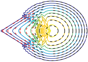
which relates the behaviour in space and time of the perturbation. In the absence of deposition process, the temporal growth rate $\mathrm {Im}(\omega )$ does not depend on $u$, which influences only the advection of perturbations. The response in the absence of deposition is characterized by concentric circles (see figure 3a) that propagate from a centre that is advected away with the linear advection velocity $u$. The maximum value of the thickness increases exponentially with time (see figure 3b). In the following, we rescale the fluid thickness using the maximum value, knowing that the growth in amplitude is exponential. The isovalues of the temporal growth rate are concentric circles propagating from $(k_x,k_y)=0$ (see figure 3c), i.e. the growth rate is isotropic. The growth rate increases for small wavenumbers, reaches a maximum at $k=1/\sqrt {2}$, then decreases and becomes negative for $k>1$, the cut-off wavenumber. Therefore, the linearized dynamics does not show any preferential direction for the growth of perturbations, which are advected away.

Figure 3. Two-dimensional linear impulse response in the absence of substrate variations, for $u=0.77$. (a) Response in the physical space at $t=200$. (b) Temporal evolution of the maximum value of the response. (c) Temporal growth rate, as a function of $k_x$ and $k_y$. The red dot denotes the initial impulse location.

3.2. Large-time behaviour of the impulse response

In this section, we analytically study the linear impulse large-time response. So as to better characterize the response observed in figure 3(a) and understand the structure when the deposition process will be introduced, together with the differences with the case in the absence of substrate variations, we present the theoretical tools to describe the impulse response of a linear system, the Green function $\tilde {g}$. The method is a generalization of the classical one-dimensional approach (Brevdo Reference Brevdo1991; Carriere & Monkewitz Reference Carriere and Monkewitz1999; Juniper Reference Juniper2007). For $t\rightarrow \infty$, the Green function asymptotically reads

(3.3)\begin{equation} \tilde{g}(x,y,t) \sim \hat{g} \exp\left[\mathrm{i}\left(k_x x +k_y y -\omega t \right)\right]/t, \quad t\rightarrow \infty \end{equation}

where the streamwise wavenumber $k_x$, the spanwise wavenumber $k_y$ and the complex frequency $\omega$ are varying in space and time, via their dependence on so-called rays $x/t$ and $y/t$. The evaluation of the asymptotic properties along the rays ($x/t=\mathrm {const},y/t=\mathrm {const}$) for $t \rightarrow \infty$ is performed using the method of the steepest descent in the complex $k_x$ and $k_y$ planes. At large times, the dominating contribution with group velocity ($x/t,y/t$) is given by the following saddle points in the complex $k_x$ and $k_y$ planes:

(3.4)\begin{equation} \frac{\partial \omega^{\prime \prime}}{\partial k_x}=\frac{\partial \omega^{\prime \prime}}{\partial k_y}=0, \end{equation}

where $\omega ^{\prime \prime }=\omega -k_x x / t-k_y y / t$. The resulting values of $k_x$, $k_y$ and $\omega ^{\prime \prime }$ for each ray $(x/t,y/t)$ allow to reconstruct the linearized dynamics of the wavepacket.

The evaluation of the saddle points is performed in MATLAB, by using the built-in function ‘fsolve’ that solves simultaneously for the saddle points in the two complex planes $k_x$ and $k_y$ using the dispersion relation (3.2). The initialization is based on the solution of the one-dimensional case documented in Brun et al. (Reference Brun, Damiano, Rieu, Balestra and Gallaire2015) for $(x/t,y/t)=(0,0)$, which corresponds to the maximum temporal growth rate in the dispersion relation and is a contributing saddle point according to Barlow, Helenbrook & Weinstein (Reference Barlow, Helenbrook and Weinstein2017). The solution at different $(x/t,y/t)$ is obtained using as initial guess the previously calculated value.

The asymptotic properties for $u=0.77$ are reported in figure 4. We report only positive values of $y/t$, since $\omega ^{\prime \prime }$, $\omega$ and $k_x$ are symmetric with respect the axis $y/t=0$, while $k_y$ is antisymmetric. The isocontours of the spatio-temporal growth rate $\sigma =\mathrm {Im}(\omega ^{\prime \prime })$ (figure 4a) are concentric circles that propagate from a centre at $(x/t=u,y/t=0)$. The maximum value $\sigma =1/12$ is located at the centre and coincides with the maximum of the dispersion relation (3.2). Increasing the distance from the centre, the values of $\sigma$ decrease. At a distance from the centre of $\approx 0.54$, the spatio-temporal growth rate is zero, and becomes negative at larger distances. The full description of the asymptotic properties is completed with the results in figure 4(b–f). The real part of the complex frequency $\mathrm {Re}(\omega )$ (figure 4b) is characterized by positive values in the upstream part of the wavepacket and by negative values in the downstream part. The transition region where $\mathrm {Re}(\omega )=0$ is located at $x/t=u$, and the transition becomes more abrupt whilst decreasing $y/t$, with a discontinuity at $y/t=0$. This discontinuity can be observed also in the real parts of the streamwise (figure 4d) and spanwise (figure 4f) wavenumbers, while the corresponding imaginary parts (figure 4c,e) are zero.

Figure 4. Large-time asymptotic properties of the two-dimensional linear impulse response in the absence of deposition, for $u=0.77$, as functions of $x/t$ and $y/t$. The coloured isocontour plots represent the analytical results of § 3.2. (a) Spatio-temporal growth rate. (b) Real part of the complex frequency. (c) Imaginary part of the streamwise wavenumber. (d) Real part of the streamwise wavenumber. (e) Imaginary part of the spanwise wavenumber. (f) Real part of the spanwise wavenumber. The black dashed line identifies the region $\sigma =0$. The red dashed lines denote the results of the post-processing algorithm described in § 4.

According to the spatio-temporal analysis approach (Van Saarloos Reference Van Saarloos2003), the front is defined by the region where $\sigma =0$. In the one-dimensional case the front is defined only by a value of $x/t$, while in two dimensions by couples $(x/t,y/t)$. From the analysis, it results that the front of the wave packet is a circle of radius $\approx 0.54$ centred around $(x/t=u, y/t=0)$. This value agrees with the absolute-convective instability transition predicted by Brun et al. (Reference Brun, Damiano, Rieu, Balestra and Gallaire2015) for the one-dimensional case. Since the centre of the wavepacket is located at $x/t=u$, and the front is a circle of radius $0.54$ (independent of $u$), the first case in which the spatio-temporal growth rate is non-negative at $x/t=0$ is when $u=0.54$. As the linear advection velocity decreases, the unstable region invades negative values of $x/t$, i.e. upstream of the initial impulse position, and the flow is said to be absolutely unstable (Huerre & Monkewitz Reference Huerre and Monkewitz1990).

The above-performed analytical spatio-temporal analysis could be in principle performed also in the presence of the deposition process. Nevertheless, the possible presence of multiple saddle points to be identified, and the discrimination of upstream and downstream propagating branches related to the different saddle points, make the problem arduous to tackle theoretically. We therefore propose a numerical approach, which presents some originalities and interesting perspectives. The analytical results of this section will be used to validate the numerical algorithm and as a reference point when restoring the coupling with the deposition process.

4.1. The Riesz transform and the monogenic signal

In this section, we introduce the mathematical tools necessary for the spatio-temporal analysis of the impulse response from the linear simulations. Numerical analyses of the linear impulse response have been already performed in the literature (Delbende & Chomaz Reference Delbende and Chomaz1998; Delbende et al. Reference Delbende, Chomaz and Huerre1998; Gallaire & Chomaz Reference Gallaire and Chomaz2003), where the asymptotic properties along one single direction were studied. The study of the asymptotic properties of a one-dimensional wavepacket is based on the introduction of the analytic signal (Delbende et al. Reference Delbende, Chomaz and Huerre1998), which is the complex continuation of a real signal. The analytic signal is derived using the Hilbert transform, which corresponds to a phase shift of $-90^{\circ }$ and $+90^{\circ }$, respectively, to the positive and negative Fourier components of a function $g(x)$, i.e. the Hilbert transformed signal reads

(4.1)\begin{equation} {\mathcal{H}}{g}(x)=H_x\star g(x), \end{equation}

where $H_x$ is a filter characterized by the Fourier transform $\hat {H}_x(k_x)=-\mathrm {i}\,\mathrm {sgn}(k_x)$, and the symbol $\star$ denotes the convolution operator. In the Fourier domain, the convolution becomes a product, such that the Fourier transform of the Hilbert transformed signal reads $\hat {\mathcal {H}}{g}=-\mathrm {i}\,\mathrm {sgn}(k_x)\hat {g}(k_x)$, where $\hat {g}$ is the Fourier transformed signal. The analytic signal gives access to the envelope and the phase of the wavepacket; indeed, as an alternative to its representation as the two components function $\boldsymbol {g}_a(x)=(g(x), \mathcal {H} g(x))$, the complex function ${g}_a(x)=g(x) +\mathrm {i}\mathcal {H} g(x)$ can be defined. The analytic signal $g_a$ is said to be the complex continuation of the real signal and can be rewritten in terms of amplitude and phase ${g}_a(x)=A \exp (\mathrm {i} \xi )$, where $A$ is the instantaneous amplitude (i.e. the envelope) and $\xi$ the phase of the complex signal. As explained in detail in § 4.2, knowledge of the envelope of the wavepacket is necessary to analyse the spatial and temporal growth rates, while the phase gives access to the spatial and temporal frequencies.

Our work aims to generalize the approach of Delbende et al. (Reference Delbende, Chomaz and Huerre1998) to the two-dimensional case, in the presence of two spatial propagation directions. We introduce the monogenic signal, the multidimensional generalization of the analytic signal (Unser et al. Reference Unser, Sage and Van De Ville2009). In the literature, there are several attempts to generalize the analytic signal in two dimensions (Bulow & Sommer Reference Bulow and Sommer2001; Felsberg & Sommer Reference Felsberg and Sommer2001; Hahn Reference Hahn2003). In this work, we use the definition given by Unser et al. (Reference Unser, Sage and Van De Ville2009), based on the multidimensional generalization of the Hilbert transform, the Riesz transform (Stein & Weiss Reference Stein and Weiss2016). In the two-dimensional case, in analogy to the Hilbert transform, the Riesz operator transforms the scalar signal $g({x,y})$ to the vector signal $\boldsymbol {g}_R({x,y})$ that reads

(4.2)\begin{equation} \boldsymbol{g}_{{R}}({x,y})=\left(\begin{array}{@{}l@{}}{g_{{R}1}({x,y})} \\ {g_{{R}2}({x,y})}\end{array}\right)=\left(\begin{array}{@{}l@{}}{H_{x} * g({x,y})} \\ {H_{y} * g({x,y})}\end{array}\right), \end{equation}

where $*$ denotes the convolution operator in two dimensions. The functions $H_{x}$ and $H_y$ are two filters characterized, respectively, by the Fourier transforms $\hat {H}_{x}({k_x,k_y})=-\mathrm {i} k_{x} /k$ and $\hat {H}_{y}({k_x,k_y})=-\mathrm {i} k_{y} /k$, and they are the generalization of the one-dimensional filter to two spatial directions. In an analogy to the Hilbert transformed signal, we consider a definition of the Riesz transformed signal that combines the two components in one scalar signal (Unser et al. Reference Unser, Sage and Van De Ville2009) as follows:

(4.3)\begin{equation} \mathcal{R} g({x,y}) =g_{{R}1}({x,y}) + \mathrm{i}g_{{R}2}({x,y}), \end{equation}

which in the Fourier domain reads

(4.4)\begin{equation} \hat{\mathcal{R}} g({k_x,k_y}) = \frac{\left(-\mathrm{i} k_{x}+k_{y}\right)}{k} \hat{g}({k_x,k_y}), \end{equation}

where $\hat {g}$ is the two-dimensional Fourier transform of the signal. Note that at $k_x=k_y=0$ the Fourier transform of the Riesz transformed signal is singular and the regularization assumes zero value at the origin. We then introduce the monogenic signal as the three-components function, as follows:

(4.5)\begin{equation} {\boldsymbol{g}_m}(x,y)=(g(x,y), \ \operatorname{Re}(\mathcal{R} g(x,y)), \ \mathrm{Im}(\mathcal{R} g(x,y)))=\left(g, g_{R1}, g_{R2}\right). \end{equation}

According to Unser et al. (Reference Unser, Sage and Van De Ville2009), the relation between the Riesz and the Hilbert transforms along the $(x,y)$ directions can be seen as the equivalent between the definition of gradient and partial derivatives. The quantity $r=\sqrt {g_{R1}^{2}+g_{R2}^{2}}=|\mathcal {R}g|$ identifies the maximum response of the directional Hilbert operator

(4.6)\begin{equation} \max _{\psi}\left\{\mathcal{H}_{\psi} g\right\}=\max _{\psi}\left\{\operatorname{Re}\left(\textrm{e}^{-\mathrm{i} \psi} \mathcal{R} g\right)\right\} \end{equation}

along the direction $d_\psi$ given by the angle $\psi =\mathrm {atan}(g_{R2}/g_{R1})$. The instantaneous amplitude (i.e. the envelope of the signal) is given by

(4.7)\begin{equation} {A}=\sqrt{g^{2}+g_{R1}^{2}+g_{R2}^{2}} \end{equation}

and the phase by

(4.8)\begin{equation} \xi=\mathrm{atan}\left(\sqrt{g_{R1}^{2}+g_{R2}^{2}}/g\right). \end{equation}

This decomposition allows us to write the monogenic signal along $d_\psi$ in the form

(4.9)\begin{equation} \tilde{g}(x,y,t)={A}\exp(\mathrm{i}\xi). \end{equation}

The amplitude ${A}$ represents the envelope of the signal and $\xi$ the phase along the direction $d_{\psi }$. Note that (4.9) is valid only when amplitude and phase of the signal can be demodulated (Delbende et al. Reference Delbende, Chomaz and Huerre1998). This is valid when the variations of the envelope occur at a scale much larger than that governing the oscillations. The representation in (4.9) is the two-dimensional equivalent of the analytic signal (Delbende et al. Reference Delbende, Chomaz and Huerre1998) and identifies in $\tilde {g}$ the complex continuation of the two-dimensional real signal $g$.

4.2. Large-time asymptotic properties

In this section, we derive the asymptotic properties of the wavepacket by following the same procedure outlined in Delbende et al. (Reference Delbende, Chomaz and Huerre1998). According to § 3.2, the complex Green function reads

(4.10)\begin{equation} \tilde{g} \sim \exp\left[\mathrm{i}\left(k_x x +k_y y -\omega t\right)\right]/t, \end{equation}

where the asymptotic properties $k_x$, $k_y$ and $\omega$ depend on $x/t$ and $y/t$.

The linear simulations of the impulse response give as a result the real signal $g(x,y)$. We thus recover the complex Green function by the analytic continuation of $g$, i.e. the monogenic signal $\tilde {g}$, as follows:

(4.11)\begin{equation} \tilde{g} \sim \exp\left[\mathrm{i}\left(k_x x +k_y y -\omega t\right)\right]/t = {A}\exp(\mathrm{i}\xi), \end{equation}

where ${A}=|\tilde {g}|$ and $\xi =\mathrm {arg}(\tilde {g} )$. Thus, by exploiting the last expression, we can use the monogenic signal $\tilde {g}$ to evaluate the asymptotic properties of the wavepacket. The spatio-temporal growth rate

(4.12)\begin{equation} \sigma=\mathrm{Im}(\omega^{\prime\prime})=\mathrm{Im}(\omega)-\mathrm{Im}(k_x)x/t -\mathrm{Im}(k_y)y/t=\mathrm{Im}(\omega)-\mathrm{Im}(k_x)v_x -\mathrm{Im}(k_y)v_y, \end{equation}

which represents the growth of a perturbation along a ray of group velocities $(x/t,y/t)=(v_x,v_y)$, is obtained by applying the logarithm operator to the absolute value of (4.11)

(4.13)\begin{equation} |\tilde{g}| \sim \exp(\sigma t)/t = {A} \quad \rightarrow \quad \sigma t - \ln(t) \sim \ln(A) \end{equation}

and thus by evaluating the derivative with respect to time of the resulting expression (for $x/t=\mathrm {const},y/t=\mathrm {const}$) as

(4.14)\begin{equation} \sigma(x=v_{x}t,y=v_{y}t) \sim \frac{\mathrm{d}}{{\mathrm{d}t}}\ln(A(x=v_{x}t,y=v_{y}t,t))+\frac{1}{t}. \end{equation}

The definition of the spatio-temporal growth rate (4.12) allows us to evaluate the imaginary part of the streamwise and spanwise wavenumbers at each ray $(x/t,y/t)=(v_x,v_y)$ (see appendix B for details), i.e.

(4.15)\begin{gather} \mathrm{Im}(k_x(x=v_{x}t,y=v_{y}t))=-\partial_{v_{x}} \sigma, \end{gather}

(4.16)\begin{gather} \mathrm{Im}(k_y(x=v_{x}t,y=v_{y}t))=-\partial_{v_{y}} \sigma. \end{gather}

The real parts of the spatial wavenumbers are retrieved by considering (4.11) and exploiting the definition of phase:

(4.17)\begin{gather} \mathrm{Re}(k_x(x=v_{x}t,y= v_{y}t)) \sim \partial_x \xi(x=v_{x}t,y=v_{y}t), \end{gather}

(4.18)\begin{gather} \mathrm{Re}(k_y(x=v_{x}t,y= v_{y}t)) \sim \partial_y \xi(x=v_{x}t,y=v_{y}t). \end{gather}

Alternatively, still exploiting the logarithm of (4.11), a direct evaluation of the real and imaginary parts of the spatial wavenumbers from the complex monogenic signal can be performed giving

(4.19)\begin{gather} k_x\sim-\mathrm{i}\partial_x\ln(\tilde{g}(x=v_{x}t,y=v_{y}t)), \end{gather}

(4.20)\begin{gather} k_y\sim-\mathrm{i}\partial_y\ln(\tilde{g}(x=v_{x}t,y=v_{y}t)). \end{gather}

In this work, we adopted this technique to evaluate the streamwise and spanwise wavenumbers. The temporal growth rate is obtained from the knowledge of the spatio-temporal growth rate and the imaginary part of the wavenumbers, as follows:

(4.21)\begin{equation} \mathrm{Im}(\omega)=\sigma+\mathrm{Im}(k_x) x / t+\mathrm{Im}(k_y) y / t. \end{equation}

The real part of the complex frequency is, by definition, the temporal derivative of the phase $\xi$, i.e.

(4.22)\begin{equation} \mathrm{Re}(\omega)(x/t,y/t,t) \sim - \partial_t \xi(x/t,y/t,t). \end{equation}

Note that in this case the derivative with respect to the time is evaluated in a relatively short time interval, without following the rays $x/t=v_{x}$ and $y/t=v_{y}$ (Delbende et al. Reference Delbende, Chomaz and Huerre1998). Moreover, the sign of the spatial frequencies cannot be recovered from the analysis, since we are post-processing a real signal. In the following, we will consider positive values for the real parts of the complex frequency and spatial wavenumbers.

4.3. Numerical procedure and validation

The analytical developments derived in the previous sections aim at describing the asymptotic behaviour for $t \rightarrow \infty$ using numerical simulations at finite times. In addition, (4.9) assumes that the amplitude and the phase of the signal subject to the Riesz transform can be demodulated, i.e. that a separation of scales between the variations of the envelope and the oscillations subsists. In this section, we verify the numerical procedure and the validity of the assumptions using as a test case the analytical solution described in § 3.2. The post-processing algorithm is validated against the theoretical results of the impulse response in the absence of substrate variations. The numerical implementation is based on MATLAB. The linear response is computed using (3.1) subjected to a Gaussian initial condition that mimics the Delta function behaviour, as follows:

(4.23)\begin{equation} \eta(x,y,0)=\eta^{0}(x,y,0)=\exp\left[-(x^{2}+y^{2})/2\varsigma^{2}\right], \end{equation}

with $\varsigma =1$; no appreciable changes in the response have been observed for $\varsigma <1$.

The numerical steps for the post-processing are the following. We apply the two-dimensional Fourier transform to the linear response at different times via the built-in MATLAB function ‘fft2’. We obtain the Riesz transformed signal by (4.4). The inverse Fourier transform is applied (via the built-in MATLAB function ‘ifft2’) and we build the monogenic signal in the physical space, for different times, according to (4.9). We evaluate the spatio-temporal growth rate by (4.12), using the monogenic signals evaluated at different times. We then obtain the streamwise and spanwise wavenumbers by a finite difference expression of (4.19) and (4.20), and then the temporal growth rate by a finite difference approximation of (4.21). Finally, the real part of the complex frequency is recovered from (4.22) using the computed monogenic signals at different times.

We evaluate the derivatives using first-order finite differences. A convergence analysis has been performed on the number of collocation points and the order of the finite differences for the derivatives, and we observed the convergence of the results already for a domain of $L_x=L_y=1000$ and $N_x=N_y=1001$. The odd number of points is necessary to have also the zero frequency $k_x=k_y=0$, where the transfer function of the Riesz transform is singular and has to be regularized imposing the zero value. The results are averaged at different times (Lerisson Reference Lerisson2017). We consider a time step of $\Delta t=15$ for the evaluation of the spatio-temporal growth rate, from $t=200$ to $t=350$. At each time, the real part of the complex frequency is evaluated using a time step of $\delta t=0.01$ (Delbende et al. Reference Delbende, Chomaz and Huerre1998).

In figure 4 we also report a comparison of the post-processing algorithm (red dashed lines) against the results of the saddle points analysis (coloured isocontours). The results agree with those obtained from the saddle-points approach. The spatio-temporal growth rate (figure 4a) is well described by the numerical post-processing, and the front of the wavepacket is well captured. The other variables well agree with the analytical solution. Figure 5 shows the results for the temporal properties and the streamwise wavenumber as functions of $x/t$, at $y/t=0$. The comparison reveals a good agreement, except in the centre of the wavepacket where the analytical solution is discontinuous. The difference can be imputed to a transient effect at the centre of the wavepacket, which is reduced as time increases. Note that the analytical solution of § 3.2 is rigorously valid as $t \rightarrow \infty$. Nevertheless, in the numerical simulations, there is a practical limit in the final time related to the numerical noise. The maximum ratio between the smaller and greater values in the simulations is limited to $16$ decades, for the double precision (Trefethen & Bau Reference Trefethen and Bau III1997). Therefore, we cannot go beyond the final time above defined, i.e. $t=350$. Despite the presence of a discontinuity in the centre of the wavepacket, the numerical procedure well captures the structure of the solution. Concerning the spatio-temporal growth rate, the maximum error from the theoretical value is around $\varDelta =2 \times 10^{-3}$, which means a percentage error of $2.5\,\%$. The edges of the wavepacket agree well with the analytical solution. We conclude that our post-processing algorithm is able to capture the spatial structure of the asymptotic properties, making it suitable for the study of the impulse response in the presence of the deposition process.

Figure 5. Comparison of the long-time asymptotic properties of the two-dimensional linear impulse response in the absence of deposition ($u=0.77$) as functions of $x/t$, for $y/t=0$. The solid lines and the dots denote the analytical (§ 3.2) and numerical approaches (§ 4), respectively. (a) Spatio-temporal growth rate, imaginary and absolute value of the real part of the complex frequency. (b) Imaginary and absolute value of the real part of the streamwise wavenumber. The black dashed line denotes the values of $\sigma$.

5.1. Dispersion relation

In this section, we briefly study the temporal stability properties in the presence of the deposition process. Following the linear stability analysis approach, we assume the normal mode expansion

(5.1)\begin{equation} \left[\eta, \eta^{0}\right]^{\textrm{T}}=\left[\eta, \eta^{0}\right]^{\textrm{T}} \exp\left[\mathrm{i}\left(k_x x +k_y y -\omega t\right)\right]. \end{equation}

It is worth underlining that this decomposition for the substrate thickness assumes that the temporal growth due to the presence of the flat film is much slower than the one related to the Rayleigh–Taylor instability. The deposition constant ${C}$ describes the growth in the absence of patterns in the fluid film. The characteristic time scale of this process has to be large enough so as the variations of the baseflow are negligible as the instability occurs. Under these conditions, a separation of scales between the speleothem growth and the Rayleigh–Taylor instability subsists. Since $C$ is already non-dimensionalized with the characteristic time scale of the Rayleigh–Taylor instability, we restrict ourselves to the case $C<10^{-3}$. In these conditions, we can safely assume the ansatz (5.1).

We introduce the normal mode decomposition in the equations for the linearized dynamics (2.8), leading to the dispersion relation which relates the complex frequency $\omega$ to the wavenumbers $(k_x,k_y)$ for the coupled hydrodynamic-deposition problem

(5.2)\begin{equation} \omega=\frac{\omega^{H}}{2} \pm \sqrt{\left(\frac{\omega^{H}}{2}\right)^{2} -\frac{\check{C}}{3}\left(k^{2}-k^{4}\right)}, \end{equation}

where $\omega ^{H}$ is the complex frequency in the absence of substrate variations, (3.2).

The dispersion relation (5.2) is analogous to the one reported in Bertagni & Camporeale (Reference Bertagni and Camporeale2017) in the absence of inertial effects. Two branches of the dispersion relation are identified. One branch is always damped while the other one tends to the hydrodynamic case as ${C}$ goes to zero. The dynamics is governed by two non-dimensional parameters, the linear advection velocity $u$ and the deposition constant ${C}$. A preliminary analysis of the influence on the dispersion relation for a large range of $u$ did not show any appreciable effect on the temporal growth rate of perturbations, for fixed deposition constants $10^{-10}<{C}<10^{-3}$. For computational reasons, it is not convenient to consider extremely large values of $u$, as large as those that can be found in limestone caves ($l_c/h_N \sim 270$, i.e. $u \sim 10^{2}$), since the advection of perturbations will require the use of unrealistic extremely large computational domains for the numerical simulations, while the physics of the travelling wavepacket would not change significantly. For these reasons we focus on the case $u=0.77$ and $\theta =55^{\circ }$, and we study the effect of the deposition constant ${C}$.

In figure 6 we report the temporal growth rate $\mathrm {Im}(\omega )$ as a function of $(k_x,k_y)$, for different values of the deposition constant. For ${C}=10^{-5}$, the temporal growth rate is analogous to the case without deposition, and no appreciable anisotropies are observed. At very high values of the deposition constant, ${C}=10^{-3}$, the isovalues are concentric circles in most of the $(k_x,k_y)$ plane, but there is a small region located close to $k_x=0$ where the growth rate is slightly higher (the difference is of order $10^{-3}$). The isotropy is broken, and spanwise structures (rivulets) experience a slightly larger growth than the streamwise structures (waves), as already pointed out in Bertagni & Camporeale (Reference Bertagni and Camporeale2017).

Figure 6. Temporal growth rate $\mathrm {Im}(\omega )$ from the dispersion relation in the presence of deposition (5.2) as a function of $(k_x,k_y)$ for (a) ${C}=10^{-5}$ and (b) ${C}=10^{-3}$.

Nevertheless, the small anisotropy in the dispersion relation may be not sufficient to completely characterize a linear selection of streamwise structures in the deposition process that should arise also for low values of the deposition constant, in the range defined by Camporeale (Reference Camporeale2015). Moreover, the complex form of the dispersion relation does not highlight how the deposition process influences the spatio-temporal growth of perturbations, and thus it does not shed light on the physics underlying the phenomenon. We therefore focus on the response of the system to a localized initial perturbation, i.e. the Green function.

5.2. Numerical impulse response

In this section, we focus on the spatio-temporal analysis of the linear impulse response, both on the substrate and in the fluid film, in the presence of the deposition process (2.8). We consider two representative values of the deposition constant which cover the physical range indicated by Camporeale (Reference Camporeale2015), ${C}=10^{-5}$ and ${C}=10^{-3}$. Figure 7 shows the linear impulse response in terms of fluid and substrate thickness, at $t=200$. We recall that in § 3 we observed that the fluid thickness response in the absence of substrate variations was characterized by concentric circles. The fluid film thickness (figure 7a,c) is characterized by a quite similar structure, albeit some differences can be highlighted. While in the downstream part (I) we observe circular isovalues for $\eta$, the pattern in the upstream part (II) is more intricate.

Figure 7. Linear impulse response (2.8) for $u=0.77$ at $t=200$. (a,b) Here ${C}=10^{-5}$; (a) fluid film and (b) substrate thickness. (c,d) Here ${C}=10^{-3}$; (c) fluid film and (d) substrate thickness. Results are rescaled with the maximum fluid thickness for visualization purposes. The red dots denote the initial impulse location.

The substrate thickness (figure 7b,d) presents similar peculiarities. The isovalues in the downstream part are circular, while in the upstream part streamwise aligned structures are present. The region in which streamwise structures dominate roughly corresponds to the region upstream of the maximum film thickness. These structures grow as higher values of the deposition constant are considered. As a consequence, we observe a more perturbed pattern in the fluid film.

The isotropy breaking in the fluid film is related to the presence of deposited streamwise structures in the upstream part of the wavepacket. While in the downstream part the hydrodynamics dominate the pattern with an isotropic structure reminiscent of the case without deposition (§ 3), observed also in the substrate thickness, in the upstream part we observe an interaction between the hydrodynamics and the deposition process.

As the impulse travels, it leaves behind a substrate pattern characterized by predominant streamwise structures. From a physical point of view, this may be explained by the fact that waves are structures that are advected away with the flow, while rivulets are not. Furthermore, it has to be remembered that the deposition law is linear with the film thickness (see (2.6)). The growth of substrate disturbances is superposed with the classical growth in the presence of a flat film, i.e. the substrate thickness is always increasing, but this is not obvious for the perturbation $\eta ^{0}$. Since waves are travelling structures (i.e. they are oscillating at fixed locations), the linearized deposition law is sequentially increasing and decreasing the substrate perturbation with respect to the linear growth in time, then leading to a much smaller effect on the deposition process. On the contrary, rivulets are not travelling structures. The substrate perturbation always increases or decreases, since there is no advection of the fluid structures along the spanwise direction. As a consequence of the passage of the wavepacket, predominant streamwise structures are deposited on the substrate.

5.3. Large-time behaviour of the impulse response

In this section we apply the post-processing algorithm, introduced in § 4, to the two cases of figure 7. According to the decomposition of (5.1), the analysis of the asymptotic properties can be applied to both variables. The difference in the patterns observed in figure 7 are related to the different eigenvectors $[\hat {\eta },\hat {\eta }^{0}]$. In the following, we consider the fluid thickness for the evaluation of the asymptotic properties. However, the observed physical results are not affected by this choice.

In figure 8(a) we report the spatio-temporal growth rate obtained from the post-processing algorithm, for ${C}=10^{-5}$. The spatio-temporal growth rate is greater than zero in a region downstream of the initial impulse position (III). The unstable region spreads in the $(x/t,y/t)$ plane within a region roughly defined by a front angle $\varphi \simeq 36.5^{\circ }$. In the downstream part of the wavepacket (I), we observe circular isovalues of the spatio-temporal growth rate, which decreases moving away from the value of $(x/t=u,y/t={0})$. The two regions interact in the region just upstream of the maximum spatio-temporal growth rate position (II). The real part of the complex frequency (figure 8b) presents the same structure of the spatio-temporal growth rate. In the region downstream of the initial impulse location, both the real and imaginary parts of the complex frequency are close to zero.

Figure 8. Asymptotic properties from the post-process algorithm (§ 4), for $u=0.77$ and ${C}=10^{-5}$. (a) Spatio-temporal growth rate. (b) Real part of the complex frequency. (c) Imaginary part of the streamwise wavenumber. (d) Real part of the streamwise wavenumber. (e) Imaginary part of the spanwise wavenumber. (f) Real part of the spanwise wavenumber.

A complete characterization of the asymptotic behaviour of the impulse response requires also the evaluation of the spatial asymptotic properties $k_x$ and $k_y$, which are reported in figure 8(c–f). Downstream of the initial impulse location, all the spatial properties isovalues are approximately rays that propagate from the initial impulse position. Interestingly, the real part of the streamwise wavenumber is very small, i.e. $\mathrm {Re}(k_x) \sim 10^{-2}$. Moreover, at $y/t=0$, $\mathrm {Re}(k_y) \simeq 1/\sqrt {2}$, while in the absence of deposition it was zero except in the singular point at the centre of the wavepacket.

The same behaviour is found in the case ${C}=10^{-3}$ (reported in appendix C), but the front downstream of the initial impulse position is more curved. Moreover, the region in which the two patterns interact is displaced downstream.

The present analysis reveals that there are three regions in the spatio-temporal impulse response. Region (I) is characterized by asymptotic properties whose distribution is very similar to the case in the absence of substrate variations, studied in § 3.2. In region (III) streamwise structures dominate. Since in the region just downstream of the initial impulse location the complex growth rate is close to zero, the pattern is almost steady. Moreover, the analysis of the spatial asymptotic properties reveals that streamwise aligned structures dominate, since $\mathrm {Re}(k_x)\sim 10^{-2}$ and $\mathrm {Re}(k_y) \sim 1/\sqrt {2}$. The other spatial asymptotic properties are almost constant for $y/x=\mathrm {const}$ since the isovalues are rays that propagate from the initial impulse position. In region (II), the two regions (I) and (III) interact, and it is best observed in the fluid film response (figure 7), where the substrate presents non-negligible values of the thickness compared with the fluid film. In this region, due to the high values of the fluid film thickness, we observe a strong deposition and an increase of the substrate thickness.

We therefore identified two linear mechanisms that could lead to the emergence of draperies structures on the substrate. First, the advection of oscillating perturbations along the streamwise direction promotes the deposition of drapery-like structures rather than wave patterns on the substrate (ripples). This interpretation confirms the observation of slightly higher growth rates for spanwise perturbations in the two-dimensional dispersion relation of Bertagni & Camporeale (Reference Bertagni and Camporeale2017). This first mechanism strongly enhances the growth of draperies structures in the region just upstream of the maximum thickness, which is advected away with time. The second mechanism was highlighted thanks to the post-processing algorithm, which shows the presence of another region in which the perturbation grows, absent in the case without substrate variations of § 3.2. The presence of the initial defect that grows without being advected, creates a quasi-steady region characterized by streamwise structures both in the fluid film and on the substrate. The second mechanism appears to be dominant in the regions in which the isotropic response has been advected away. In the following, we investigate the hydrodynamic origin of this second source of anisotropy.

6.1. Numerical response and large-time asymptotics

In this section, we provide an additional analytical insight to better understand the physical mechanisms underlying the response in the presence of the deposition process. We consider the linear response of the thin film (2.8) in the presence of a steady defect (i.e. $C=0$) of the form

(6.1)\begin{equation} \eta^{0}(x,y,t)=\exp[-x^{2}/2-y^{2}/2], \end{equation}

together with the initial condition for the fluid thickness, $\eta (x,y,0)=0$.

The wavepacket (figure 9), in the downstream part (I), is characterized by the isotropic structure typical of the temporal response (figures 3 and 7), as described in detail in § 3.2. Nevertheless, in the upstream part (II) we observe streamwise structures more pronounced than in the case of the impulse response in presence of deposition (described in § 3.2), since the initial condition differs from a steady defect as it is characterized by an impulse both in the fluid film and on the substrate.

Figure 9. Linear fluid film response (2.8) (rescaled with the maximum value) in the presence of a steady defect (i.e. $C=0$) located at $(x=0,y=0)$, for $u=0.77$, (a) $t=100$ and (b) $t=200$. The black dots denote the steady defect location.

The asymptotic properties (figure 10) resulting from the post-processing algorithm present a spatial structure analogous to the case in the presence of deposition reported in figure 8. In region (III), downstream of the initial impulse location, the isovalues are rays that propagate from $(x/t,y/t)=(0,0)$. Both real and imaginary parts of the complex frequency are zero in the region downstream of the steady defect, and the real part of the streamwise wavenumber is of order $10^{-2}$.

Figure 10. Long-time asymptotic properties from the post-process algorithm (§ 4) of the two-dimensional linear response to steady defect in the absence of deposition, for $u=0.77$. (a) Spatio-temporal growth rate. (b) Real part of the complex frequency. (c) Imaginary part of the streamwise wavenumber. (d) Real part of the streamwise wavenumber. (e) Imaginary part of the spanwise wavenumber. (f) Real part of the spanwise wavenumber.

The steady defect analysis confirms that the structure of the wavepacket is mainly driven by hydrodynamic effects. Moreover, the region downstream of the obstacle is steady because $\omega =0$ and originates from the presence of the steady defect. Since the asymptotic properties are rays that propagate from the centre, the properties of the steady pattern are constant at fixed $y/x$. This invariance suggests that the response can be evaluated in the context of a steady pattern asymptotic analysis, introduced in Lerisson et al. (Reference Lerisson, Ledda, Balestra and Gallaire2020) for the front analysis of a propagating steady wavepacket, known as spatio-spatial stability analysis.

6.2. The two-dimensional steady Green function

In this section, we analytically derive the Green function for a steady defect. The approach is based on the spatio-temporal analysis introduced in § 3.2, but we focus on the growth in space of a steady wavepacket. We can thus make an analogy to the classical one-dimensional analysis (Van Saarloos Reference Van Saarloos2003): the $(x,y)$ directions play the role of space and time.

Following Hayes et al. (Reference Hayes, O'Brien and Lammers2000), we introduce the total free surface elevation $\eta _{{t}}=\eta +\eta ^{0}$. We seek for the solution of the following problem:

(6.2)\begin{equation} u \partial_{x} \eta_{{t}}+\tfrac{1}{3}\left[\nabla^{2} (\eta_{{t}})+\nabla^{4} (\eta_{{t}})\right]=-u \partial_{x} \eta^{0}=f(x,y). \end{equation}

The impulse is located in the position $y/x=0$, i.e. the Green function $\tilde {g}_s(x,y)$ solves the steady problem,

(6.3)\begin{equation} u \partial_{x} \eta_{{t}}+\tfrac{1}{3}\left[\nabla^{2} (\eta_{{t}})+\nabla^{4} (\eta_{{t}})\right]=\delta (x) \delta(\,y). \end{equation}

The solution in the presence of a localized defect $\eta _{{t}}$ is found using the property of the Green function, i.e. $\eta _{{t}}=\tilde {g}_s * f$, where $*$ is the convolution operator. Since we consider the response to a steady localized defect $f(x,y)=\partial _x [\delta (x) \delta (\,y)]$. Using the properties of the Delta function and integrating by parts, we obtain the solution that reads

(6.4)\begin{equation} \eta_{{t}}=u \partial_x \tilde{g}_s(x,y). \end{equation}

The solution $\tilde {g}_s$ is found using the same approach of the spatio-temporal stability analysis, where now we have the direction $x \rightarrow \infty$. The Green function for steady defect can be expressed as

(6.5)\begin{equation} \tilde{g}_s(x,y) \sim \hat{g} \exp(k_x x + k_y y) /\sqrt{x} \sim \hat{g} \exp(k_x^{\prime} x)/\sqrt{x}, \end{equation}

where $k_x^{\prime }=k_x+k_y (\,y/x)$. The solution reads

(6.6)\begin{equation} \eta_{{t}}=u \partial_x \tilde{g}_s(x,y) \sim \mathrm{i}u k_x \exp[\mathrm{i}(k_x x +k_y y)]/\sqrt{x}, \end{equation}

i.e. the asymptotic properties of the total elevation $\eta _{{t}}$ wavepacket are the same as the Green function for $x \rightarrow \infty$.

The spatio-spatial analysis is implemented similarly to the spatio-temporal stability analysis outlined in § 3.2. We look for the steady (i.e. $\omega =0$) dispersion relation (3.2) saddle points of $k_x^{\prime }=k_x+k_y (\,y/x)$ in the complex $k_y$ plane, varying $y/x$. The resulting asymptotic properties define the response for each $y/x$. The method is numerically implemented in MATLAB; we solve for the saddle point using the built-in function ‘fsolve’. The initial guess is given by the maximum in the steady dispersion relation (3.2) for $y/x=0$, which is a contributing saddle point according to Barlow et al. (Reference Barlow, Helenbrook and Weinstein2017).

In figure 11 we report the spatial asymptotic properties as functions of $y/x$. The spatio-spatial growth rate $\mathcal {K}=-\mathrm {Im}(k_x^{\prime })$ (figure 11a) is initially positive and decreases with $y/x$. Beyond the critical value of $y/x =0.74$ it becomes negative. Both the real and imaginary parts of the streamwise wavenumber (figure 11b) are negative and decrease with $y/x$, in opposition to the real and imaginary parts of the spanwise wavenumber (figure 11c), which are positive and increase with $y/x$.

Figure 11. Analytical asymptotic properties for the steady two-dimensional Green function. (a) Spatio-spatial growth rate as a function of $y/x$. (b) Streamwise wavenumber and (c) spanwise wavenumber resulting from the analytical steady response, as functions of $y/x$.

The unstable region in the $(x,y)$ plane is located where the spatio-spatial growth rate is positive. At low values of $y/x$, i.e. close to $y=0$, we observe a positive spatio-spatial growth rate, i.e. perturbations are growing (remember that one writes $\eta _{{t}} \sim \exp \left [\mathrm {i}(k_x x +k_y y)\right ]$). When $\mathcal {K}=0$ we define the value of $y/x$ beyond which perturbations are damped, that is $y/x=0.74$. This value of $y/x$ defines a ray in the $(x,y)$ plane, that corresponds to an angle with respect to the $x$ axis of $\varphi \simeq 36.5^{\circ }$, in agreement with the front observed in figures 8 and 10.

These results can be easily visualized in figure 12, in which we report the real part of the total free surface elevation and the asymptotic properties in the $(x,y)$ plane, in a similar fashion to the previous plots for the spatio-temporal response. The total free surface elevation is characterized by predominant streamwise structures. The steady Green function is growing moving away from the obstacle, in strong contrast to the case of the flow over an incline, in which it is decaying (Hayes et al. Reference Hayes, O'Brien and Lammers2000; Kalliadasis et al. Reference Kalliadasis, Bielarz and Homsy2000; Decré & Baret Reference Decré and Baret2003). The streamlines of the wavevector $\boldsymbol {k}=(\mathrm {Re}(k_x),\mathrm {Re}(k_y))$ (red dashed lines in figure 12a) are parallel to the $y$ direction at $y=0$ and slightly bend upstream with $y$. This slight variation is related to the negative value of the real part of the streamwise wavenumber. The bending of the wavevector streamlines imply that the wavefronts (black dashed lines in figure 12a), orthogonal to the wavevector directions, tend to slightly diverge from the centre going downstream.

Figure 12. Results of the spatio-spatial analysis in the $(x,y)$ plane. (a) Real part of the total free surface elevation $\eta _{{t}}$ obtained from the asymptotic properties. The red and black dashed line denote the streamlines of the wavevector $\boldsymbol {k}=(\mathrm {Re}(k_x),\mathrm {Re}(k_y))$ and the wavefronts, respectively. (b) Spatio-spatial growth rate, (c) imaginary and (d) real parts of the streamwise wavenumber, (e) imaginary and (f) real parts of the spanwise wavenumber. The red line denotes the value of $y/x$ for which $\mathcal {K}=0$.

We now consider the spatio-temporal response observed in § 6.1. In the steady regions, the spatio-temporal growth rate (§ 3.2) $\sigma =\mathrm {Im}(\omega ) -\mathrm {Im}(k_x) x/t -\mathrm {Im}(k_y) y/t=\mathrm {Im}(\omega ) +\mathcal {K}x/t$ coincides with the spatio-spatial growth rate rescaled with $x/t$, i.e. $\sigma =\mathcal {K} x/t$, since $\omega =0$. In figure 13 we show the spatio-temporal growth rate obtained from the numerical simulation compared with analytical values of $\sigma$ and $\mathcal {K}x/t$, respectively, obtained from the spatio-temporal (§ 3.2) and spatio-spatial approaches, for $t=350$. The comparison shows a good agreement between spatio-spatial theory and numerical post-processing in the region downstream of the steady defect. Moreover, the numerical spatio-temporal response agrees well with the spatio-temporal results, in the region downstream of $x/t=u$.

Figure 13. Linear response to a steady defect: spatio-temporal growth rate from the post-process algorithm of § 4 (coloured isocontours) and from the saddle points approach of § 3.2 (black isocontours) and spatio-spatial growth rate (changed of sign) from the analytical steady approach of § 6.2 (red isocontours).

We report in figure 14 a comparison of the spatial asymptotic properties, at $y/t=0$. Also in this case, the results are in good agreement; the values of $\mathrm {Re}(k_y)$ are converging to the analytic values as $x$ increases. The small difference in the values is due to the fact that we are considering not large enough values of $x$ close to the obstacle. The saddle point analysis is rigorously valid for $x \rightarrow \infty$, and in this case the steady response is present in the range $0<x<175$ for the considered time ($t=350$), which explains the small difference.

Figure 14. Comparison of streamwise (a) and spanwise (b) wavenumbers obtained from the post-process algorithm of § 4 (dots), the analytical approach (coloured solid lines) for the response to a steady defect of § 6.2 and the analytical results of the spatio-temporal analysis of § 3.2 (black solid lines), on the ray $y/t=0$.

Our analysis shows that the temporal response to a steady defect is characterized by the presence of the steady and unsteady contributions which interact. The steady contribution, which originates from the presence of the steady defect, is not advected away and spreads in the domain as the streamwise coordinate increases. The presence of an initial perturbation gives rise also to a temporal response that is advected away. If we wait for enough time, eventually the temporal response is no longer present in the field and only the steady response survives, which is characterized by streamwise-aligned structures.

We then conclude that the emergence of streamwise structures both on the fluid film and on the substrate in the region just downstream of the initial impulse location is related to the presence of defects on the substrate and it has a linear hydrodynamic origin. This mechanism is predominant in the regions in which the temporal response has been advected away. In the context of morphogenesis of draperies, we thus argue that the response in the presence of the deposition process contains as fundamental ingredients two hydrodynamic effects, one related to the isotropic unsteady response in the absence of substrate variations, and the other one related to the steady response in the presence of a localized defect in the substrate. The deposition process couples these two different hydrodynamic mechanisms, giving rise to predominant draperies structures on the substrate.