


1. Introduction
Among all the possible modalities of transport of solid particles in a carrier fluid, saltation (Andreotti Reference Andreotti2004), that is successions of particle jumps over a bed that can be either rigid or erodible, is generally accepted as the most common when dealing with windblown sand and of crucial importance in determining the morphology of dunes (Sauermann, Kroy & Herrmann Reference Sauermann, Kroy and Herrmann2001; Charru, Andreotti & Claudin Reference Charru, Andreotti and Claudin2013). Hence, most of the works on saltation concern a grain-to-fluid density ratio of order  $2\times 10^3$ and take the fluid to be turbulent, as in Aeolian transport on Earth (e.g. Bagnold Reference Bagnold1941; Owen Reference Owen1964; Iversen & Rasmussen Reference Iversen and Rasmussen1999; Creyssels et al. Reference Creyssels, Dupont, El Moctar, Valance, Cantat, Jenkins, Pasini and Rasmussen2009; Durán, Claudin & Andreotti Reference Durán, Claudin and Andreotti2011; Kok et al. Reference Kok, Parteli, Michaels and Karam2012; Ho et al. Reference Ho, Valance, Dupont and Ould El Moctar2014; Valance et al. Reference Valance, Rasmussen, Ould El Moctar and Dupont2015).
Saltation of solid particles in a turbulent fluid at grain-to-fluid density ratio of order 2, as in the aquatic environment on Earth (Fernandez Luque & Van Beek Reference Fernandez Luque and Van Beek1976; Abbott & Francis Reference Abbott and Francis1977; van Rijn Reference van Rijn1984; Niño & García Reference Niño and García1998; Ancey et al. Reference Ancey, Bigillon, Frey, Lanier and Ducret2002), 40, as on Venus (Iversen & White Reference Iversen and White1982; Greeley et al. Reference Greeley, Iversen, Leach, Marshall, Williams and White1984), 200, as on Saturn's moon Titan (Burr et al. Reference Burr, Bridges, Marshall, Smith, White and Emery2015), and  $10^5$, as on Mars (Iversen et al. Reference Iversen, Pollack, Greeley and White1976; Iversen & White Reference Iversen and White1982), have also been experimentally investigated in water channels or wind tunnels.
Discrete numerical simulations of interacting solid particles subjected to forces transmitted by the surrounding fluid (Tsuji, Kawaguchi & Tanaka Reference Tsuji, Kawaguchi and Tanaka1993) are a powerful tool to analyse the physics of sediment transport and have been largely applied in the recent years to systematically investigate the influence of the particle size and the density ratio on particle saltation in turbulent fluids (Durán, Andreotti & Claudin Reference Durán, Andreotti and Claudin2012; Pähtz et al. Reference Pähtz, Durán, Ho, Valance and Kok2015; Pähtz & Durán Reference Pähtz and Durán2020; Ralaiarisoa et al. Reference Ralaiarisoa, Besnard, Furieri, Dupont, Ould El Moctar, Naaim-Bouvet and Valance2020).
These numerical tools solve Newton's laws of motion for the individual particles, while treating the fluid as a continuum for which Reynolds-averaged balance equations are phrased. The discrete-continuum (DC) numerical simulations provide a large amount of data, some of which would be unattainable in experiments. Also, the required closures for modelling the particle–particle and particle–fluid interactions and the fluid internal stresses are transparent and can be easily turned on or off. Thus, DC simulations are ideal to, e.g. test how much essential physics is captured by mathematical models of saltation at a higher level of abstraction.
Countless continuum descriptions of saltation exist (see the extensive reviews from Durán et al. Reference Durán, Claudin and Andreotti2011; Kok et al. Reference Kok, Parteli, Michaels and Karam2012; Valance et al. Reference Valance, Rasmussen, Ould El Moctar and Dupont2015; Pähtz et al. Reference Pähtz, Clark, Valyrakis and Durán2020). Among those, we recently proposed a simple toy model that combines the classic idea (Bagnold Reference Bagnold1941; Owen Reference Owen1964; Sauermann et al. Reference Sauermann, Kroy and Herrmann2001) of assuming that all particles follow the same trajectory, despite the severe criticism of Andreotti (Reference Andreotti2004), with a description of the rebound of particles shot onto rigid or erodible beds drawn from experiments and numerical simulations (Beladjine et al. Reference Beladjine, Ammi, Oger and Valance2007; Crassous, Beladjine & Valance Reference Crassous, Beladjine and Valance2007). If applied to steady saltation, the resulting identical trajectories must be periodic. We solved this periodic trajectory (PT) model both numerically and analytically and show qualitative and quantitative agreement against experiments and DC simulations of steady saltation in turbulent fluids (Jenkins & Valance Reference Jenkins and Valance2014; Berzi, Jenkins & Valance Reference Berzi, Jenkins and Valance2016; Berzi, Valance & Jenkins Reference Berzi, Valance and Jenkins2017).
Saltation of particle immersed in a viscous fluid in the absence of turbulence has received much less attention (Charru & Mouilleron-Arnould Reference Charru and Mouilleron-Arnould2002; Ouriemi, Aussillous & Guazzelli Reference Ouriemi, Aussillous and Guazzelli2009; Aussillous et al. Reference Aussillous, Chauchat, Pailha, Médale and Guazzelli2013; Seizilles et al. Reference Seizilles, Lajeunesse, Devauchelle and Bak2014), although it is one of the possible modes of transport of sand in oil pipes (Leporini et al. Reference Leporini, Terenzi, Marchetti, Corvaro and Polonara2019), in which sand depositions would lead to a significant loss of the pipe transport capacity (Dall'Acqua et al. Reference Dall'Acqua, Benucci, Corvaro, Leporini, Cocci Grifoni, Del Monaco, Di Lullo, Passucci and Marchetti2017). From the scientific point of view, focusing on saltation in the absence of turbulence would also permit us to capture the essence of the physics of the particle motion without the complexity and the somewhat arbitrariness that modelling turbulence necessarily implies.
Here, we first formulate a PT model for the steady saltation of particles over a horizontal, rigid rough bed driven by the shearing flow of a viscous non-turbulent fluid. In doing this, for the sake of clarity, we neglect the role of lubrication forces in damping the collisions of the particles with the bed and the possibility of particle–particle interactions above the bed. The PT model reduces to a system of differential equations that we solve both numerically and, with some further simplifying assumptions, analytically. Linear stability analysis permits us to prove that some of the solutions obtained for a given strength of the shearing flow and number of particles in the system are actually unstable to small perturbations.
We also perform two-dimensional (2-D) DC simulations of steady saltation over horizontal rigid rough beds in which we keep constant the intensity of the shearing flow, the particle–fluid density ratio and the particle size and vary the number of particles in the domain. In the DC simulations, as in the PT model, we do not include lubrication forces when the particles interact and turn off the possibility of collisions above the bed. These assumptions permit us to clearly identify the strengths and the weaknesses of the PT model. Ignoring mid-fluid collisions is justified as long as the particle concentration is small. In the context of turbulent saltation over an erodible bed, the transition between a collision-free saltation regime and a saltation regime modified by mid-fluid collisions has been evidenced numerically and experimentally (Ralaiarisoa et al. Reference Ralaiarisoa, Besnard, Furieri, Dupont, Ould El Moctar, Naaim-Bouvet and Valance2020). The authors showed that there exists a regime of Shields parameters where the sand transport can be described in a relevant manner by a collision-free saltation model. However, at high Shields number, mid-air collisions start to play a substantial role and the collision-free saltation model breaks down. We believe that this picture persists in viscous saltation over a rigid bed.
The paper is organized as follows: in § 2 we describe the PT model and the DC numerical simulations; in § 3, we report detailed comparisons in terms of global and local quantities between the numerical and analytical solutions of the PT model and the measurements in the DC simulations; § 4 offers some concluding remarks and hints at future works on the subject.
2. Flow configuration and methods
We focus on steady saltation of identical spheres (in three dimensions) or disks (in two dimensions) of diameter  $d$ and mass density
  $\rho _p$ over a horizontal bumpy rigid base driven by the laminar shearing flow of a fluid of mass density
  $\rho _f$ and molecular viscosity
  $\eta _f$ in the presence of gravity (
 $g$ is the gravitational acceleration) and in the absence of turbulence. We take
  $x$ and
  $y$ to be the horizontal and vertical directions (we neglect variation in the spanwise direction);
  $U$ is the horizontal component of the fluid velocity, while
  $\xi _x$ and
  $\xi _y$ are the horizontal and vertical components of the particle velocity. We use superscripts ‘
 $+$’ and ‘
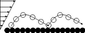
 $-$’ to refer to quantities relative to the ascending and descending portions of the particle trajectory (figure 1).

Figure 1. Sketch of saltation over a rigid bumpy bed.
We make all quantities dimensionless using  $d$,
$d$,  $\rho _p$ and the reduced gravity
  $g(\rho _p-\rho _f)/\rho _p$, so that, e.g. the velocities are expressed in units of
  $\sqrt {gd(\rho _p-\rho _f)/\rho _p}$, the particle fall velocity. Then, the inverse of the dimensionless fluid viscosity is the fall Stokes number
  $St=\rho _p\sqrt {g(\rho _p-\rho _f)/\rho _p}d^{3/2}/\eta _f$, a measure of the relative magnitude of the particle inertia to the fluid viscous forces.
The intensity of the shearing fluid is quantified by the distant fluid shear stress far from the base, that, in dimensionless terms, is the Shields parameter  $Sh$ (Jenkins & Hanes Reference Jenkins and Hanes1998). The fluid exerts a linear drag on the single particle that we characterize through the drag coefficient
  $C_D=18/St$. Finally, we fix the mass hold-up in the system,
  $M$, that is the particle mass per unit basal area.
2.1. The PT model: differential equations and numerical solution
The system of differential equations governing the periodic particle trajectory and the fluid velocity profile is almost identical to that derived for periodic saltation in turbulent fluids (Jenkins & Valance Reference Jenkins and Valance2014; Berzi et al. Reference Berzi, Jenkins and Valance2016) in which we distinguish two species of particles, depending whether their motion is ascending or descending, and one fluid carrier phase
 \begin{gather} \xi_y^\pm\frac{\mbox{d}\xi_x^\pm}{\mbox{d}y} = C_D\left(U-\xi_x^\pm\right); \end{gather}
 \begin{gather}\xi_y^\pm\frac{\mbox{d}\xi_y^\pm}{\mbox{d}y}={-}1-C_D\xi_y^\pm; \end{gather}
 \begin{gather}\xi_y^\pm\frac{\mbox{d}\kern0.7pt x^\pm}{\mbox{d}y} = \xi_x^\pm; \end{gather}
 \begin{gather}\left(1-c^+{-}c^-\right)\frac{\mbox{d}U}{\mbox{d}y} = St\,S; \end{gather}
 \begin{gather}\frac{\mbox{d}m}{\mbox{d}y} = c^+{+}c^-; \end{gather}
 \begin{gather}\frac{\mbox{d}\left(c^+\xi_y^+\right)}{\mbox{d}y} = 0. \end{gather}
Note that, for numerical convenience, the Lagrangian (2.1)–(2.3) are phrased as functions of  $y$ instead of time
  $t$. However, there is one-to-one correspondence between
  $y$ and
  $t$ in the ascending and descending parts of the trajectory, respectively. Equations (2.1)–(2.2) are the particle momentum balances in the horizontal and vertical directions. Equation (2.3) governs the horizontal position of the particles, while (2.4) is the constitutive expression for the fluid viscous shear stress
  $S$, different from what was assumed in turbulent conditions (Jenkins & Valance Reference Jenkins and Valance2014). Equation (2.5) determines the distribution of the partial mass hold-up,
  $m=\int _0^y\,{{\rm d}y} (c^++c^-)$, with
  $c^+$ (respectively
  $c^-$) the particle volume concentration of ascending particles (respectively descending particles). Finally, (2.6) indicates that, in steady conditions, the mass flux of an ascending particle must be independent of the vertical position.
The fluid shear stress is determined from the fluid horizontal momentum balance as
 \begin{equation} S= Sh-s, \end{equation}
where  $s$ is the particle shear stress:
 \begin{equation} s \equiv{-}\left(c^+\xi_y^+\xi_x^+{+}c^-\xi_y^-\xi_x^-\right). \end{equation}
The steady condition implies that the mass flux of ascending and descending particles must balance
 \begin{equation} c^+\xi_y^+{=} -c^-\xi_y^-, \end{equation}
and be constant along  $y$. The concentration
  $c$ at a given height is simply given by the sum of
  $c^+$ and
  $c^-$.
The distribution of the twelve unknowns  $x^+$,
  $x^-$,
  $\xi _x^+$,
  $\xi _x^-$,
  $\xi _y^+$,
  $\xi _y^-$,
  $U$,
$U$,  $m$,
$m$,  $S$,
$S$,  $s$,
$s$,  $c^+$ and
  $c^-$ is determined by solving the nine differential equations (2.1)–(2.6) with the three auxiliary relations (2.7)–(2.9) and the nine boundary conditions
  $x^+(0)=0$,
  $x^-(0)=L$,
  $x^+(H)=x^-(H)$,
  $\xi _x^+(H)=\xi _x^-(H)$,
  $\xi _y^+(H)=\xi _y^-(H)=0$,
  $U(0)=0$,
  $m(0)=0$ and
  $m(H)=M$; where
  $H$ and
  $L$ are the trajectory height and length, respectively. Note that the total mass hold-up
  $M$ represents the mass of particles per unit area of the bed and is a control parameter of the system that has to be prescribed.
The determination of  $H$ and
  $L$ requires two additional boundary conditions, relating the velocities after and before the impact with the bumpy base (Oger et al. Reference Oger, Ammi, Valance and Beladjine2005; Beladjine et al. Reference Beladjine, Ammi, Oger and Valance2007; Crassous et al. Reference Crassous, Beladjine and Valance2007)
 \begin{equation} \sqrt{\xi_x^+(0)^2+\xi_y^+(0)^2}=e \sqrt{\xi_x^-(0)^2+\xi_y^-(0)^2}, \end{equation}
and
 \begin{equation} \xi_y^+(0)={-}e_y\xi_y^-(0), \end{equation}
where the coefficients of restitution depend solely on the impact angle  $\theta$, the angle between the incident trajectory and the horizontal, in the absence of lubrication forces. Their expressions (Beladjine et al. Reference Beladjine, Ammi, Oger and Valance2007; Pähtz et al. Reference Pähtz, Clark, Valyrakis and Durán2020) are
  $e\equiv a-b\sin \theta$ and
  $e_y\equiv a_y/\sqrt {\sin \theta }-b_y$. (We used the modified expression of
  $e_y$ proposed by Pähtz et al. (Reference Pähtz, Clark, Valyrakis and Durán2020) to get the correct asymptotic behaviour when
  $\theta$ vanishes.) Only three of the four numerical coefficients
  $a$,
$a$,  $b$,
$b$,  $a_y$ and
  $b_y$ are actually independent, for, when
  $\theta =90^\circ$,
  $e$ must equal
  $e_y$ and their values depend on the particle and base material properties and geometry.
The numerical solution of the PT model is obtained using the bvp4c function in Matlab: the inputs of the model are the Stokes number,  $St$, the Shields parameter,
  $Sh$, the mass hold-up,
  $M$, and the numerical coefficients in the rebound laws (2.10) and (2.11). From the numerical solution we then determine the horizontal mass flux per unit width of the bed as
  $Q=\int _0^H(c^+\xi _x^++c^-\xi _x^-)\,{{\rm d}y}$.
2.2. The PT model: approximate analytical solution
We obtain an approximate analytical solution of the PT model by following an approach similar to that employed for periodic saltation in a turbulent fluid (Berzi et al. Reference Berzi, Jenkins and Valance2016, Reference Berzi, Valance and Jenkins2017).
With respect to the numerical solution of the PT model, we make the further assumptions that the fluid velocity profile is linear (this should be true only in the limit of vanishing mass hold-up) and that the impact angle is small, so that  $\theta \approx \sin \theta \approx \tan \theta$. The details of the derivation and the analytical formulas that describe the characteristics of the PTs are reported in Appendix A.
For mathematical convenience only, we use the vertical rebound velocity,  $\xi _y^+(0)$, rather than the mass hold-up,
  $M$, as an input parameter. However,
  $M$ can be treated as the independent variable when plotting the results, given that there is a one-to-one relation with the vertical rebound velocity (see (A25)).
2.3. The DC simulations
We carry out two-phase numerical simulations based on a discrete element method for the particle dynamics coupled to a continuum Stokes description of hydrodynamics, as developed by Durán et al. (Reference Durán, Andreotti and Claudin2012).
The particle motion is described by a Lagrangian approach according to which the particle labelled  $p$ obeys the following dimensionless equations:
 \begin{gather} \frac{\mbox{d}\boldsymbol{\xi^p}}{\mbox{d}t}={-} \boldsymbol{e}_y + \sum_{q} \boldsymbol{f}_c^{p,q} + \boldsymbol{f}_{drag}^p, \end{gather}
 \begin{gather}I \frac{\mbox{d}\boldsymbol{\omega^p}}{\mbox{d}t}= \frac{1}{2} \sum_{q} \boldsymbol{n}^{p,q} \times \boldsymbol{f}_c^{p,q}, \end{gather}
where  $\boldsymbol {\xi ^p}$ and
  $\boldsymbol {\omega ^p}$ are the translational and angular velocity vectors of particle
  $p$, respectively;
  $\boldsymbol {e}_x$ and
  $\boldsymbol {e}_y$ are the horizontal and vertical unit vectors, respectively;
  $\boldsymbol {f}_c^{p,q}$ is the dimensionless contact force between particles
  $p$ and
  $q$;
$q$;  $\boldsymbol {f}_{drag}^p = C_D [ (U-\xi _x^p) \boldsymbol {e}_x - \xi _y^p \boldsymbol {e}_y ]$ is the dimensionless drag force exerted by the fluid on the
  $p$-particle;
  $I=1/10$ is the moment of inertia of a sphere; and
  $\boldsymbol {n}^{p,q}$ is the unit vector along the contact direction.
The contact force  $\boldsymbol {f_c}$ has components normal,
  $f_{c,n}$, and tangential,
  $f_{c,t}$, to the plane of contact. In the normal direction, the particles interact via a linear spring dashpot, so that
  $f_{c,n}=(k_n \delta + \gamma _n v_n)$, where
  $k_n$ is the spring stiffness,
  $\delta$ the overlap between the compliant spheres,
  $\gamma _n$ the viscous damping coefficient and
  $v_n$ the normal component of the relative translational particle velocities. The negative of the ratio between the normal relative velocity before and after the collision is the coefficient of normal restitution
  $e_n$. If the values of
  $e_n$ and
  $k_n$ are prescribed,
  $\gamma _n$ is deduced from the following relation:
  $\gamma _n= ({{\rm \pi} }/{6}) \sqrt {{12k_n/{\rm \pi} }/{(1+{\rm \pi} ^2/\ln (e_n)^2)}}$. The tangential force
  $f_{c,t}$ is described via a Coulomb friction model regularized through a viscous damping:
  $f_{c,t}=-min(\mu f_{c,n}, \gamma _t v_t) sign(v_t)$, where
  $\mu$ is the Coulomb friction coefficient,
  $v_t$ the relative slip velocity at contact and
  $\gamma _t$ the tangential viscous damping coefficient. The values chosen for the parameters
  $k_n$,
  $\gamma _n$,
  $\gamma _t$ and
  $\mu$ are reported in table 1.
Table 1. Parameters in the contact model in dimensionless form.

The fluid motion is solved by an Eulerian description based on the Stokes equations. We assume that the vertical component of the fluid velocity is zero, so that only the horizontal momentum balance is required, and neglect the inertial terms
 \begin{equation} \frac{\mbox{d}S}{\mbox{d}y} = F_x, \end{equation}
where  $F_x= c \langle \sum _{p\in [y;y+\mbox {d}y]} C_D(U-\xi _x^p) \rangle /\langle \sum _{p\in [y;y+\mbox {d}y]}1 \rangle$, with
  $\langle \,\cdot \,\rangle$ denoting ensemble averaging, represents the
  $x$-component of the average volume force exerted on the fluid by the particles whose centres are located in the horizontal slice between
  $y$ and
  $y+\mbox {d}y$. The volume of these particles divided by the volume of the horizontal slice gives the local concentration
  $c$.
$c$.
The integration of (2.14) reads
 \begin{equation} S = Sh-\int_y^\infty F_x\,\mbox{d}y, \end{equation}
where the infinite upper bound of the integral means that all moving grains located above  $y$ must be accounted for. Once the distribution
  $S(y)$ of the fluid shear stress is determined, the distribution of the horizontal fluid velocity can then be obtained from the integration of (2.4), with the no-slip boundary condition
  $U=0$ at
  $y=0$, as
 \begin{equation} U = St\int_0^yS\,\mbox{d}y. \end{equation}
 The simulated system is quasi-two-dimensional with a streamwise length equal to  $5120$ particle diameters and a transverse length equal to one diameter. We have checked that a fourfold increase in the streamwise length of the domain has a negligible influence on the outcomes. We use spherical particles with a polydispersity of
  ${\pm }10\,\%$ and adjust their number in the system to obtain the desired value of mass hold-up
  $M$.
$M$.
Periodic boundary conditions are employed in the streamwise direction. The domain is not upper bounded, while the lower boundary is composed of a layer of immobile particles, characterized by the same parameters as in table 1, in close contact (rigid, bumpy bed). As mentioned, we suppress the possibility of particle–particle interactions above the bed, that is, we take  $\boldsymbol {f_c}^{p,q}=\boldsymbol {0}$ in (2.12) and (2.13), if neither of the two particles
  $p$ and
  $q$ belong to the bed.
Operatively, at every time step, we integrate (2.12) and (2.13) for every particle in the system and determine its new velocity (and therefore position). We then use this information to update the profiles of fluid shear stress and horizontal velocity through (2.15) and (2.16) and proceed with the next time step until we reach a steady state, that is, when the horizontal mass flux averaged over a window of 100 time steps is stationary. Initially, the fluid profile is taken to be linear and corresponds to the unperturbed profile that one would have obtained in the absence of particles. The particles are initially placed on a horizontal row located at a distance  $2d$ from the particle rigid bed, with a constant inter-particle distance equal to
  $2d$ and zero initial velocity. Despite the fact that the initial positions of the particles are close to the bed, the rebounds with the rigid bumpy base are able to make the particles reach large heights (see next section). We checked that the final state is independent of the initial conditions as long as the number of particles in the flow does not override the transport capacity of the flow. If the mass hold-up surpasses the capacity of the flow, particles may deposit on the bed and we enter the so-called deposition regime. In this regime, hysteretic effects may be observed: the final state may be extremely sensitive to the initial conditions. This regime, although interesting, is beyond the scope of the current article.
3. Results and comparisons
Given that the PT model requires the specification of the rebound laws, we first determine the dependence of the coefficients of restitution  $e$ and
  $e_y$ on the impact angle
  $\theta$ for the type of particles and the geometry of the rigid bumpy bed adopted in the DC simulations. To do this, we perform discrete element simulations in the absence of interstitial fluid (Oger et al. Reference Oger, Ammi, Valance and Beladjine2005) in which we shoot soft spheres towards the rigid bumpy bed described in § 2.2 and measure the particle velocities before and after the impact. Changing the angle between the incident sphere and the bed (several measurements are carried out for every impact angle to obtain statistically robust averages) permits us to plot
  $e$ and
  $e_y$ as functions of
  $\theta$ (figure 2). The fit to the numerical data from the impact simulations gives
  $a=0.86$,
  $b=0.1$,
  $a_y=1.44$ and
  $b_y=0.68$. We also performed some simulations with less dissipative particles and confirm that that would lead, as expected, to higher values of
  $e$ and
  $e_y$ for given
  $\theta$.

Figure 2. Coefficients of restitution characterizing the collision with the rigid bumpy bed as functions of the impact angle.
Given that the contact model is not velocity dependent, we expect that the rebound laws inferred from shooting a projectile onto a rigid bed in the absence of any fluid can accurately describe the bed collision process of particles transported by a shearing viscous fluid. The measurements of  $e$ and
  $e_y$ vs
  $\theta$ obtained from the impacts of the particles with the bed in our DC simulations confirm, indeed, the validity of the rebound laws (figure 2). The small differences between the impact and the saltation DC simulations are due to the fact that the absence of shearing permits to achieve a better accuracy of the measured velocity before and after the impact. It can be noticed that the range of impact angles in the DC simulations is rather narrow with respect to that of the shooting simulations.
We now employ the obtained dependence of the rebound coefficients of restitution on the impact angle to solve the PT model for  $St=100$, roughly corresponding to sand particles in water on Earth,
  $Sh=0.05$ (sufficiently larger than the transport threshold for having a significant range of steady solutions) and various mass hold-ups (numerical solution) or various vertical rebound velocities (analytical solution). The DC simulations were carried out at the same values of the fall Stokes number and Shields parameter by changing
  $M$.
$M$.
Unlike the PT model, particles in the DC simulations are characterized by a statistical distribution of trajectories. We first compare quantities averaged over all the trajectories in the DC simulations in a time interval of at least 2000 time steps after the steady state is attained with the predictions of the PT model. Then, we describe the characteristics of the statistical distribution of the trajectories, in view of future improvements of the PT model.
3.1. Averaged variables
Figure 3 depicts the horizontal mass flux as a function of the mass hold-up. We immediately notice that the PT model predicts a non-monotonic relation between  $Q$ and
  $M$, characterized by a maximum value for the mass hold-up below which solutions exist. This maximum divides the
  $Q$–
$Q$– $M$ curve into an upper and a lower branch. Interestingly, the measurements in the DC simulations only appear to follow the upper branch. The lack of measurements from the DC simulations near the lower branch hints at the possibility that these solutions of the PT model are actually unstable. The maximum mass flux in the DC simulations corresponds to a critical value of the mass hold-up above which particles start to deposit over the rigid bed. This transition from saltation over rigid beds to saltation over erodible beds is beyond the scope of the present work and cannot be captured by the PT model, given the adopted boundary conditions.

Figure 3. Horizontal mass flux  $Q$ as a function of the mass hold-up
  $M$ measured in the DC simulations (squares) and obtained from the numerical (circles) and analytical (lines) solution of the PT model, when
  $St=100$ and
  $Sh=0.05$.
The numerical and analytical solution of the PT model described in the previous section permit us to formulate a relation between the rebound velocities at the beginning of two consecutive particle jumps, say the  $n$th and
  $(n+1)$th jump. This relation formally reads
  $\boldsymbol {\xi }_{n+1}^+(0)=\boldsymbol {F}(\boldsymbol {\xi }_{n}^+(0))$. The fixed point of this 2-D map corresponds to the rebound velocity of the PT. The stability of the PT can then be determined by computing the eigenvalues of the Jacobian matrix of the 2-D map at the fixed point. The PT is stable if the absolute values of the eigenvalues are smaller than one. More details about the linear stability analysis and the Jacobian matrix obtained from the analytical solution of the PT model are reported in Appendix B. The linear stability analysis confirms that the lower branch of the
  $Q$–
$Q$– $M$ curve of the PT model pertains to unstable PTs.
If we focus on the stable trajectories, we notice that, for small mass hold-ups, both the PT model and the DC simulations show a linear relation between  $Q$ and
  $M$ and are in a good quantitative agreement. Using the analytical solution of the PT model, we obtain that, for vanishing mass hold-up,
  $Q\propto St^4Sh^{3/2}M$ (see the details in Appendix C). This scaling, checked against the DC simulations (Appendix C), points to the intuitive and general observation that the horizontal mass flux at a given mass hold-up increases if either the intensity of the shearing (the Shields number) increases or the fluid viscosity (the inverse of the Stokes number) decreases: indeed, these are the quantities that govern the capability of the particles to gain momentum from the fluid through the drag force. It is interesting to notice that a linear relation between the horizontal mass flux and the mass hold-up was obtained also in the case of PTs of sand particles saltating in the turbulent atmosphere (Jenkins & Valance Reference Jenkins and Valance2014), although in that case
  $Q\propto Sh^{1/2}M$.
As the mass hold-up increases, that is, as more particles are moving, the horizontal mass flux in the DC simulations tends to saturate and the agreements between the numerical and the analytical solution of the PT model and between the PT model and the DC simulations deteriorate (figure 3). However, the qualitative trend is still well captured by the PT model. The horizontal mass flux measured in DC simulations performed with less dissipative particles (not shown here for brevity) is larger for a given mass hold-up, as expected.
Figure 4 confirms the quantitative agreement between the PT model and the DC simulations at small values of  $M$ in terms of average impact angle
  $\theta$ and absolute value of the impact velocity
  $\xi ^-$. Interestingly, at vanishing
  $M$, the stable branches of the curves exhibit a minimum and a maximum for the impact angle and velocity, respectively. The PT model reproduces the qualitative behaviour of the simulations even if the amount of saltating particles increases.

Figure 4. Average (a) impact angle and (b) impact velocity as functions of the mass hold-up, when  $St=100$ and
  $Sh=0.05$. Same legend as in figure 3.
The average height and length of the trajectories in the DC simulations are roughly half of what is predicted by the PT model at small mass hold-ups (figure 5) and decrease as  $M$ increases; while the average particle concentration and the particle shear stress at the bed are extremely well predicted (figure 6a,b) and linearly increase with
  $M$ for small mass hold-ups.

Figure 5. Average trajectory (a) height and (b) length as functions of the mass hold-up, when  $St=100$ and
  $Sh=0.05$. Same legend as in figure 3.

Figure 6. Average particle (a) concentration and (b) shear stress at the bed as functions of the mass hold-up, when  $St=100$ and
  $Sh=0.05$. Same legend as in figure 3.
3.2. Vertical profiles
The PT model is very simple and permits the understanding of the physical mechanisms in play and their relative importance in determining the average behaviour of the saltating particles. In this regard, fair comparisons between the DC simulations and the predictions of the PT model should be carried out only in terms of global quantities, such as  $Q$ and
  $M$. Nonetheless, we have shown that the PT model has some capabilities of reproducing also some local average quantities measured at the bed (figures 4 and 6). However, it would be pretentious to expect quantitative agreement between the PT model and the DC simulations in terms of distributions of local average quantities along
  $y$.
$y$.
Figure 7 depicts the average vertical profiles of fluid and particle horizontal velocity obtained from the DC simulations at four different values of the mass hold-up. As the presence of particles in the system increases, the nonlinearity of the velocity profiles becomes more pronounced. This explains why the quantitative agreement between the DC simulations and the analytical solution of the PT model, which assumes a linear distribution of  $U$ with
  $y$, deteriorates at large
  $M$. The numerical solution of the PT model is in excellent agreement with the DC simulations in terms of fluid horizontal velocity (figure 7a). Also, the particle slip velocity at the bed and the concavity of the profile of the particle horizontal velocity are well predicted by the PT model, although the latter fails in reproducing the linearity of
  $\xi _x(y)$ at small
  $M$ (figure 7b). We notice that the particle slip velocity predicted by the PT model and measured in the DC simulations is roughly independent of the mass hold-up, when the latter is small.

Figure 7. Measurements in the DC simulations (circles) and numerical solutions of the PT model (lines) for (a) fluid and (b) particle average horizontal velocity profiles when  $St=100$ and
  $Sh=0.05$ at:
  $M=1.9\times 10^{-4}$ (in blue);
  $M=1.6\times 10^{-3}$ (in orange);
  $M=1.2\times 10^{-2}$ (in yellow);
  $M=3.1\times 10^{-2}$ (in purple).
The requirement that, under steady conditions, the mass flux of ascending and descending particles must be independent of  $y$ implies, in the framework of the PT model, that the particle concentration must become infinite when the vertical particle velocity vanishes, i.e. at the peak of the PT. This is clearly unphysical and, indeed, the predictions of the PT model in terms of distribution of the average particle concentration along
  $y$ fails spectacularly when compared with the measurements in the DC simulations (figure 8a). On the other hand, at least the qualitative behaviour of the average particle shear stress with the vertical coordinate is well captured by the PT model, with even quantitative agreement with the DC simulations for both the shear stress at the bed and the maximum value of the shear stress above it (figure 8b).

Figure 8. Measurements in the DC simulations (circles) and numerical solutions of the PT model (lines) for particle average (a) concentration and (b) shear stress profiles when  $St=100$ and
  $Sh=0.05$ at:
  $M=1.9\times 10^{-4}$ (in blue);
  $M=1.6\times 10^{-3}$ (in orange);
  $M=1.2\times 10^{-2}$ (in yellow);
  $M=3.1\times 10^{-2}$ (in purple).
3.3. Statistical distributions
Our DC simulations exhibit a variety of particle trajectories, thus allowing for a statistical characterization of the saltating process.
Figure 9(a) shows the probability density function (PDF) for the impact and rebound velocities determined using the data from the DC simulation performed at  $M=1.2\times 10^{-2}$. Interestingly, there are two peaks in the PDF of the impact velocity, indicating the presence of two different families of saltating particles, one much more energetic than the other. We have checked that this is not a consequence of the regular geometry of the rigid bed, given that we have obtained similar, bi-modal PDFs in DC simulations (not shown here for brevity) carried out with bumpiness provided by a bottom layer of immobile particles in close contact, but with a random size distribution.

Figure 9. Probability density function of (a) impact and (b) rebound velocities from the DC simulations when  $M=1.2 \times 10^{-2}$ for particles with trajectory height larger (blue bars) and smaller (yellow bars) than 15 diameters. Also shown are the means of the PDF (black lines) and the numerical solutions of the PT model (red lines).
Although the existence of different species of moving particles has been previously proposed and confirmed in the case of Aeolian sand transport over erodible beds (Andreotti Reference Andreotti2004; Durán et al. Reference Durán, Claudin and Andreotti2011; Pähtz, Kok & Herrmann Reference Pähtz, Kok and Herrmann2012), it is the first time, to our knowledge, that it has been observed in the case of particle saltation over rigid beds. Figure 9(b) indicates that the bi-modal nature of the saltation persists in the rebound velocity, after the impact with the rigid bed.
We identify the two families based upon the value of the horizontal particle velocity at the peak of the trajectory. When the trajectory height is lower (higher) than 15 diameters, in the case of  $M=1.2 \times 10^{-2}$, the particle horizontal velocity at the peak of the trajectory is larger (lower) than the fluid horizontal velocity there. Thus, the horizontal drag force on the less energetic particles mostly acts against the motion, so that the horizontal velocities at the end of the trajectory are greatly reduced (see the yellow bars in figure 9(a,b). The more energetic particles, on the other hand, experience a horizontal drag force that favours the motion for a significant portion of their trajectory, thus accelerating before the impact (see the two large peaks in the blue bars of figure 9a,b).
Figure 9(a,b) also indicates that the impact with the bed leads to a substantial mixing of the members of the two families, that have roughly the same distributions of rebound velocity. In figure 9(a), the low energy family (yellow bars) has experienced short and low trajectories before the impact while the high energy family (blue bars) has experienced long and high trajectories. After the impact, the low energy particles have a small rebound velocity, while the high energy particles have a large one, as the restitution coefficient  $e$ is close to 1. However, the rebound velocity is not the right indicator to tell whether the particle will experience a low or high trajectory for the next jump. The relevant feature is the vertical velocity after the rebound. As a matter of fact, the low energy particles which have a large vertical rebound velocity will be promoted to the high energy family for the next jump, gaining energy from the fluid. And, vice versa, the high energy particles with a small vertical rebound velocity will enter the low energy family for the next jump. In figure 9(b), representing the distribution of the norm of the rebound velocity, we have indicated with yellow bars (respectively blue bars) the particles which will have for the next jump a low (respectively high) trajectory. Those particles come both to the low and high energy family determined from the previous jump. This means that the low and high energy populations are re-mixed at each impact. This explains how steady conditions can be maintained, despite the fact that the less energetic particles lose momentum to the fluid during their jumps. The mixing of the two families due to the impact with the bed cannot be captured through the rebound laws of figure 2 that only describe average outcomes. All in all, the negligible contribution of the less energetic saltating particles to the total transport explains why the simple PT model works.
As mentioned, there is a maximum impact velocity corresponding to the case of vanishing mass hold-up, as shown in figure 4(b). Impact velocities and, therefore, rebound velocities, larger than the maximum are not allowed, leading to the skewed distributions of figure 9. Similarly, the asymmetry in the distribution of the impact angles (figure 10a) is due to the minimum  $\theta$ at vanishing
  $M$ (figure 4a).

Figure 10. Probability density function of (a) impact and (b) rebound angles from the DC simulations when  $M=1.2 \times 10^{-2}$ for particles with trajectory height larger (blue bars) and smaller (yellow bars) than 15 diameters. Also shown are the means of the PDF (black lines) and the numerical solutions of the PT model (red lines).
The intrinsic randomness of the position of the impact point on the surface of the bumpy bed is what causes the large scatter (figure 10b) of the angles of rebound,  $\psi =\tan ^{-1}[\xi _y^+(0)/\xi _x^+(0)]$, despite the fact that the impact angle
  $\theta$ is, instead, narrowly distributed. The presence of two peaks corresponding to low and high energy saltating particles is evident also in the PDFs of impact and rebound angles, once the particles are distinguished according to the height of the trajectory (figure 10). It is interesting to notice that, for low energy saltating particles, the impact and rebound angles corresponding to the peaks in the distributions are roughly equal.
The distribution of the trajectory heights (figure 11a) confirms the presence of the less energetic family of saltating particles. The less energetic species moves through small hops whose height distribution peaks at approximately four diameters; unlike for the impact velocity, however, the more energetic particles have a broader and rather uniform distribution of the maximum distance from the bed that they can reach (say, between 50 and 150 diameters). The nonlinear relation between the impact velocity and the trajectory height, made explicit in the analytical solution of the PT model (Appendix A), explains why their distributions have different shapes. Once again, values of  $H$ larger than that at vanishing
  $M$ in figure 5(a) are not allowed.

Figure 11. Probability density function of trajectory (a) heights and (b) lengths from the DC simulations when  $M=1.2\times 10^{-2}$ for particles with trajectory height larger (blue bars) and smaller (yellow bars) than 15 diameters. Also shown are the means of the PDF (black lines) and the numerical solutions of the PT model (red lines).
The PDF of trajectory lengths for the less energetic particles (figure 11b) has one clear peak at approximately 300 diameters. The distribution of trajectory lengths for the more energetic particles, instead, peaks at approximately 2000 diameters and then roughly linearly decreases as  $L$ increases. As expected, the maximum
  $L$ at vanishing
  $M$ in figure 5(b) constrains the permitted values in the statistical distribution of trajectory lengths.
4. Conclusion
We have investigated the steady, saltating motion of identical particles over a horizontal, rigid, bumpy bed driven by the shearing flow of a viscous fluid in the absence of turbulence.
We have performed 2-D DC simulations in which the particles interact with the bumpy bed via linear spring dashpots and with the carrier fluid, whose motion is determined using a mean field approach, via viscous drag and buoyancy. In the DC simulations, we have ignored lubrication forces, the possibility of collisions among the particles above the bed, the fluid inertia in the fluid momentum balance and the fluid vertical velocity.
We have compared the results of the DC simulations against the predictions of a simple model in which we assumed that all particles follow the same PTs selected by the intensity of the shearing flow and through deterministic rebound laws relating velocities before and after the impact with the bed. We have checked through discrete simulations that the presence or absence of the shearing flow has no influence on the rebound laws.
We have solved the PT model both numerically and analytically, the latter with the additional assumption that the horizontal fluid velocity profile is linearly distributed with the distance from the rigid bed. We have shown that the PT model is capable of qualitatively and quantitatively, at least for moderate values of the mass hold-up, reproducing the measurements in the DC simulations in terms of particle mass flux, mean trajectory height and length, impact and rebound velocity, concentration and shear stress at the bed. At given intensity of the shearing flow, the PT model predicts non-monotonic relations between the aforementioned quantities and the mass hold-up, in contrast with the DC simulations. However, the simplicity of the PT model has allowed us to perform a linear stability analysis and determine that the predictions of the PT model not seen in the DC simulations were actually unstable to small perturbations.
The PT model also provides profiles of fluid and particle velocity and particle shear stress that are in qualitative agreement with the DC simulations, even beyond what one might reasonably expect from such a simple approach. As expected, the PT model fails only in reproducing the concentration profile at a sufficient distance from the bed, given that the concentration must become infinite at the top of the periodic trajectory to ensure mass flux balance.
Indeed, and unlike what is assumed in the PT model, the DC simulations confirm that there is a statistical distribution of particle trajectories. The PDFs of various quantities associated with the particle trajectories are asymmetric, due to constraints that we have identified as the characteristics of the trajectories in the limit of vanishing mass hold-up. They also present two peaks, hinting at the presence of two families of trajectories associated with less and more energetic saltating particles. The PT model actually reproduces the behaviour of the more energetic particles, that are accelerated in the horizontal direction by the fluid drag and obey the rebound laws, with an impact coefficient of restitution less than one. The less energetic particles, instead, jump in a region of the flow close to the bed where the drag force is either mainly against the motion or equally favours and disfavours it. As a result, the ascending and descending parts of their trajectories are more symmetric, and the impact coefficient of restitution is close to one. The contribution of the less energetic particles to the transport is, however, small, thus explaining the success of the PT model.
Incorporating a more realistic statistical distribution of the particle trajectories into the PT model would improve its accuracy and will be the subject of future works. Further steps will regard elucidating the roles played by lubrication forces and mid-fluid collisions on particle saltation, as well as the statistical characterization of particle trajectories in turbulent shearing flows. Also, the determination of the critical mass hold-up at which particles start to deposit is a important issue to be addressed in the near future given its relation to the maximum transport capacity of the flow.
Finally, the PT model could, in principle, be extended to unsteady (non-uniform) flows under the condition that the flow varies over a characteristic time (length) scale which is much less than the mean time of flight (saltation length) of the saltating particles.
Acknowledgements
A.V. and D.B. are in debt with Professor J.T. Jenkins for meaningful insights and stimulating discussions during the preparation of the paper.
Funding
A.V. also acknowledges the financial support of Politecnico di Milano through its Senior Resident Ricerca program for visiting scholars.
Declaration of Interests
The authors report no conflict of interest.
Appendix A. Analytical solution of the PT model
Integrating the vertical momentum balance of the single particle for an observer at rest
 \begin{equation} \frac{\mbox{d}\xi_y}{\mbox{d}t}+C_D\xi_y+1=0, \end{equation}
with the boundary condition  $\xi _y=\xi _x^+(0)$ when
  $t=0$, gives
 \begin{equation} \xi_y=\frac{C_D\xi_y^+(0)+1-\exp(C_Dt)}{C_D{\rm exp}(C_Dt)}. \end{equation}
Here,  $\xi _y^+(0)$ is the vertical rebound velocity, that is, the vertical velocity after the impact with the bed. It is mathematically convenient to parametrize the analytical solution of the PT model in terms of this variable, rather than in terms of the mass hold-up, as this is the case in the numerical solution of the PT model and the DC simulations.
The vertical position of the particle as a function of time is obtained by integrating (A2) with the boundary condition  $y(0)=0$
 \begin{equation} y=\frac{\left[C_D\xi_y^+(0)+1\right]\left[1-\exp({-}C_Dt)\right]-C_Dt}{C_D^2}. \end{equation}
 The time  $t_M$ at which the particle reaches the peak in the trajectory is obtained from (A2) with
  $\xi _y=0$
 \begin{equation} t_M=\frac{\ln\left[C_D\xi_y^+(0)+1\right]}{C_D}. \end{equation}
 We determine the trajectory height,  $H$, from (A3) with
  $t=t_M$ (A4)
 \begin{equation} H=\frac{C_D\xi_y^+(0)-\ln\left[C_D\xi_y^+(0)+1\right]}{C_D^2}. \end{equation}
The time of flight during one jump can be determined by numerically by solving the following implicit equation:
 \begin{equation} t_f=\frac{\left[C_D\xi_y^+(0)+1\right]\left[1-\exp({-}C_D t_f)\right]}{C_D}, \end{equation}
obtained from (A3) with  $y=0$.
Then, the vertical impact velocity reads
 \begin{equation} \xi_y^-(0)=\xi_y^+(0)-t_f, \end{equation}
from (A2), with  $t=t_f$ (where
  $t_f$ is the total flight time), and (A6).
The vertical coefficient of restitution at the rebound can now be expressed as
 \begin{equation} e_y=\frac{\xi_y^+(0)}{t_f-\xi_y^+(0)}, \end{equation}
from (2.11) and (A7). Then, the impact angle follows from the definition of  $e_y$ as
 \begin{equation} \theta=\sin^{{-}1}\left[\left(\frac{a_y}{e_y+b_y}\right)^2\right]. \end{equation}
 If  $\theta$ is small, then
  $\sin \theta \approx \tan \theta =-\xi _y^-(0)/\xi _x^-(0)$ and the horizontal impact velocity results in
 \begin{equation} \xi_x^-(0)={-}\xi_y^-(0)\left(\frac{e_y+b_y}{a_y}\right)^2. \end{equation}
The absolute value of the impact velocity is, therefore, with (A7) and (A10),
 \begin{equation} \xi^-(0)=\left[\left(\frac{e_y+b_y}{a_y}\right)^4+1\right]^{1/2} \left[t_f-\xi_y^+(0)\right]. \end{equation}
 From the definition of the rebound coefficient of restitution  $e$ and (A9), we obtain
 \begin{equation} e=a-b\left(\frac{a_y}{e_y+b_y}\right)^2, \end{equation}
so that the absolute value of the rebound velocity,  $\xi ^+(0)=e\xi ^-(0)$, reads, with (A12)
 \begin{equation} \xi^+(0)=\left[a-b\left(\frac{a_y}{e_y+b_y}\right)^2\right] \left[\left(\frac{e_y+b_y}{a_y}\right)^4+1\right]^{1/2} \left[t_f-\xi_y^+(0)\right]. \end{equation}
The horizontal rebound velocity can now be determined as
 \begin{equation} \xi_x^+(0)=\left[\xi^+(0)^2-\xi_y^+(0)^2\right]^{1/2}. \end{equation}
Equations (A2)–(A3) provide exact analytical solutions of the vertical motion in the framework of the PT model. They allow us to derive explicit expressions for  $\xi ^-(0)$,
  $\xi ^+(0)$,
  $\xi _x^+$ and
  $H$ as a function of the vertical rebound velocity
  $\xi _y^+(0)$ and the time flight
  $t_f$, which is itself a function of
  $\xi _y^+(0)$ (cf. (A6)).
However, to proceed, we now must introduce the Lagrangian, horizontal momentum balance of the single particle
 \begin{equation} \frac{\mbox{d}\xi_x}{\mbox{d}t}=C_D\left(U-\xi_x\right), \end{equation}
which can be solved analytically only if we assume a tractable form of the fluid velocity profile  $U(y)$. In the case of periodic saltation in a turbulent fluid (Berzi et al. Reference Berzi, Jenkins and Valance2016), the fluid velocity profile was taken to be uniform. Here, instead, we assume a linear velocity profile of the form
  $U(y)=U(H)y/H$, that suits better the results of both the numerical solution of the PT model and the DC simulations. With this and (A3), (A15) becomes
 \begin{equation} \frac{\mbox{d}\xi_x}{\mbox{d}t}=\frac{U\left(H\right)}{H} \frac{\left[C_D\xi_y^+(0)+1\right]\left[1-\exp({-}C_Dt)\right]-C_Dt}{C_D}-C_D\xi_x, \end{equation}
that can be integrated, with the boundary condition  $\xi _x=\xi _x^+(0)$ when
  $t=0$, to obtain
 \begin{align} \xi_x &= \frac{U\left(H\right)}{H}\frac{C_D\xi_y^+(0)+1}{C_D^2} \left[1-C_Dt\exp({-}C_Dt)-\exp({-}C_Dt)\right]\nonumber\\ &\quad -\frac{U\left(H\right)}{H}\frac{C_Dt-1+\exp({-}C_Dt)}{C_D^2}+ \xi_x^+(0)\exp({-}C_Dt). \end{align}
The horizontal fluid velocity at  $y=H$ can be determined from (A17), with
  $\xi _x=\xi _x^-(0)$ when
  $t=t_f$
 \begin{equation} U\left(H\right)=\frac{C_D^2H\left[\xi_x^-(0)-\xi_x^+(0) \exp({-}C_Dt_f)\right]}{\left[C_D\xi_y^+(0)+1\right] \left[1-C_Dt_f\exp({-}C_Dt_f)-\exp({-}C_Dt_f)\right]+1-\exp({-}C_Dt_f)}. \end{equation}
With this, (A17) provides the value of the horizontal particle velocity at every instant.
Equation (A17) can then be integrated to provide the particle position along the  $x$-axis at every time
  $t$
$t$
 \begin{align} x &= \frac{U\left(H\right)}{H}\frac{C_D\xi_y^+(0)+1}{C_D^2} \left[\exp({-}C_Dt)\left(\frac{2}{C_D}+t\right)+t-\frac{2}{C_D}\right]\nonumber\\ &\quad -\frac{U\left(H\right)}{HC_D^2}\left[\frac{C_D}{2}t^2-t-\frac{\exp({-}C_Dt)}{C_D}+ \frac{1}{C_D}\right]-\frac{\xi_x^+(0)}{C_D}\left[\exp({-}C_Dt)-1\right]. \end{align}
Note that the solutions  $x(t)$ and
  $y(t)$ are parametrized by a single parameter, that is
  $\xi _y^+(0)$. Figure 12(a) shows
  $y/H$ and
  $x/L$ as functions of
  $t/t_f$ when
  $\xi _y^+(0)=100$. The shape of the corresponding PT is reported in figure 12(b). All the quantities appearing in (A19), such as
  $H$,
$H$,  $U(H)$,
  $\xi _x^+(0)$ and
  $t_f$, are functions of
  $\xi _y^+(0)$. So we have a family of solutions that depends solely on the vertical rebound velocity.

Figure 12. (a) Normalized vertical (solid line) and horizontal (dashed line) position of the particle as functions of the normalized time and (b) shape of the PT when  $\xi _y^+(0)=100$.
Substituting  $t=t_f$ in (A19) gives the length of the periodic trajectory
 \begin{align} L &= \frac{U\left(H\right)}{H}\frac{C_D\xi_y^+(0)+1}{C_D^2} \left[\exp({-}C_Dt_f)\left(\frac{2}{C_D}+t_f\right)+t_f-\frac{2}{C_D}\right]\nonumber\\ &\quad -\frac{U\left(H\right)}{HC_D^2}\left[\frac{C_D}{2}t_f^2-t_f- \frac{\exp({-}C_Dt_f)}{C_D}+\frac{1}{C_D}\right]\nonumber\\ &\quad -\frac{\xi_x^+(0)}{C_D}\left[\exp({-}C_Dt_f)-1\right]. \end{align}
The assumption of a linear velocity profile for the fluid permits also the evaluation of the fluid shear stress at the rigid bumpy bed as
 \begin{equation} S(0)=\frac{U\left(H\right)}{St\,H}, \end{equation}
where we have assumed  $1-c(0)\approx 1$ (as shown later, the maximum value of the concentration at the bed is of order
  $10^{-2}$). Figure 13(a) depicts the fluid shear stress at the bed as a function of the vertical rebound velocity at different values of the Stokes number. Notice that the fluid shear stress at the bed is characterized by a minimum, as was also the case for particle saltation in a turbulent fluid (Berzi et al. Reference Berzi, Jenkins and Valance2016). This has important physical implications, given that the Shields parameter
  $Sh$ determines, through (2.4), the particle shear stress at the bed as
 \begin{equation} s(0)=Sh-S(0). \end{equation}
Equation (A22) indicates that, for steady and fully developed saltation to exist, the fluid shear stress at the bed must always be less than the Shields number. Hence, each minimum in the curves of figure 13(a) represents the critical Shields number,  $Sh_c$, i.e. the minimum value of
  $Sh$ at which steady and fully developed saltation can be sustained. Figure 13(b) shows the critical Shields number as a function of the Stokes number. From (2.8) and (2.9), the concentration at the bed of the ascending particles is
 \begin{equation} c^+(0)=\frac{s(0)}{\xi_y^+(0) \left[\xi_x^-(0)-\xi_x^+(0)\right]}. \end{equation}
With this, both the horizontal mass flux per unit width of the bed
 \begin{equation} Q=\int_0^Hc\xi_x\,\mbox{d}y=\int_0^Lc^+(0)\xi_y^+(0)\mbox{d}\kern0.7pt x=c^+ (0)\xi_y^+(0)L, \end{equation}
and the mass hold-up
 \begin{align} M&=\int_0^Hc\,\mbox{d}y=\int_0^H\left(c^+{+}c^-\right) \mbox{d}y=\int_0^{t_M}c^+\xi_y^+\,\mbox{d}t+\int_{t_M}^{t_f}c^-\xi_y^-\,\mbox{d}t\nonumber\\ &=c^+(0)\xi_y^+(0)\int_0^{t_f}\mbox{d}t =c^+ (0)\xi_y^+(0)t_f, \end{align}
can, then, be evaluated. The mass hold-up  $M$ and the particle shear stress at the bed are thus both dependent on the vertical rebound velocity and Shields number.

Figure 13. (a) Fluid shear stress at the bed as a function of the vertical rebound velocity for different Stokes numbers (20, 30, 40, 50, 60 and 100) according to the analytical solution of the PT model. (b) Critical Shields number as a function of the Stokes number.
Summarizing the analytical resolution of the problem, the prescription of the vertical rebound velocity  $\xi _y^+(0)$ determines uniquely the particle trajectory, independently of the Shields number
  $Sh$, while the particle shear stress at the bed and the mass hold-up depend both on
  $Sh$ and
  $\xi _y^+(0)$. This means that a given solution of the particle trajectory can be obtained for different sets of the two variables
  $(Sh,M)$.
Appendix B. Linear stability of the PT model – analytical solution
We use the method of fixed point to determine the stability to small perturbations of the analytical solution of the PT model. We focus on the trajectory followed by a particle during the  $n$th jump and determine the components of the rebound velocity at the beginning of the
  $(n+1)$th jump from the rebound laws (2.10) and (2.11) as
 \begin{equation} \left.\begin{gathered} \xi_{x,n+1}^+(0) = \left\{\left[a+b\frac{\xi_{y,n}^-(0)}{\xi_{x,n}^- (0)}\right]^2\left[\xi_{x,n}^-(0)^2+\xi_{y,n}^-(0)^2\right] \right.\\ \quad \left.\vphantom{\left[a+b\frac{\xi_{y,n}^-(0)}{\xi_{x,n}^-(0)}\right]^2} -\left[a_y\left(-\xi_{x,n}^-(0)\xi_{y,n}^-(0)\right]^{1/2}+b_y\xi_{y,n}^- (0)\right)^2\right\}^{1/2},\\ \xi_{y,n+1}^+(0) = a_y\left[-\xi_{x,n}^-(0) \xi_{y,n}^-(0)\right]^{1/2}+b_y\xi_{y,n}^-(0), \end{gathered}\right\} \end{equation}
where we take  $\sin \theta \approx \tan \theta =-\xi _{y,n}^-(0)/\xi _{x,n}^-(0)$ in the expressions of
  $e$ and
  $e_y$.
The components of the impact velocity at the end of the  $n$th jump are determined from the components of the rebound velocity at the beginning of the same jump with (A17), with
  $t=t_f$, and (A7) as
 \begin{equation} \left.\begin{gathered} \xi_{x,n}^-(0)=\frac{U\left(H\right)}{H} \frac{C_D\xi_{y,n}^+(0)+1}{C_D^2}\left[1-C_Dt_f\exp({-}C_Dt_f)-\exp ({-}C_Dt_f)\right] \\ \quad -\frac{U\left(H\right)}{H}\frac{C_Dt_f-1+\exp({-}C_Dt_f)}{C_D^2}+\xi_{x,n}^+ (0)\exp({-}C_Dt_f), \\ \xi_{y,n}^-(0)=\xi_{y,n}^+(0)-t_f. \end{gathered}\right\} \end{equation}
Here,  $t_f$ and
  $U(H)/H$ are, from (A6), (A21)–(A23) and (A25),
 \begin{equation} \left.\begin{gathered} t_f=\frac{\left[C_D\xi_{y,n}^+(0)+1\right]\left[1-\exp\!\left(C_Dt_f\right)\right]}{C_D}, \\ \frac{U\left(H\right)}{H}=St\left\{Sh-\frac{M}{t_f}\left[\xi_{x,n}^- (0)-\xi_{x,n}^+(0)\right]\right\}. \end{gathered}\right\} \end{equation}
We now introduce perturbations (indicated with a tilde) around the periodic solution, and keep only the linear terms, so that, from (B1)–(B3)
 \begin{equation} \begin{bmatrix} \tilde{\xi}_{x,n+1}^+(0)\\ \tilde{\xi}_{y,n+1}^+(0) \end{bmatrix}=\underbrace{\begin{bmatrix} {\mathsf{A}}_{11} & {\mathsf{A}}_{12}\\ {\mathsf{A}}_{21} & {\mathsf{A}}_{22} \end{bmatrix}}_{\boldsymbol{\mathsf{A}}} \begin{bmatrix} \tilde{\xi}_{x,n}^-(0)\\ \tilde{\xi}_{y,n}^-(0) \end{bmatrix}=\underbrace{\begin{bmatrix} {\mathsf{A}}_{11} & {\mathsf{A}}_{12}\\ {\mathsf{A}}_{21} & {\mathsf{A}}_{22} \end{bmatrix}}_{\boldsymbol{\mathsf{A}}} \underbrace{\begin{bmatrix} {\mathsf{B}}_{11} & {\mathsf{B}}_{12}\\ 0 & {\mathsf{B}}_{22} \end{bmatrix}}_{\boldsymbol{\mathsf{B}}} \begin{bmatrix} \tilde{\xi}_{x,n}^+(0)\\ \tilde{\xi}_{y,n}^+(0) \end{bmatrix}, \end{equation}
where
 \begin{align} {\mathsf{A}}_{11} &= \frac{1}{2}\left\{\left[a+b\frac{\xi_{y}^-(0)}{\xi_{x}^-(0)}\right]^2 \left[\xi_{x}^-(0)^2+\xi_{y}^-(0)^2\right] \right. \nonumber\\ &\quad \left.\vphantom{\left[a+b\frac{\xi_{y}^-(0)}{\xi_{x}^-(0)}\right]^2} -\left[a_y\left(-\xi_{x}^-(0)\xi_{y}^-(0)\right)^{1/2}+b_y \xi_{y}^-(0)\right]^2\right\}^{{-}1/2} \nonumber\\ &\quad \times\left\{{-}2b\frac{\xi_{y}^-(0)}{\xi_{x}^-(0)^2} \left[a+b\frac{\xi_{y}^-(0)}{\xi_{x}^-(0)}\right] \left[\xi_{x}^-(0)^2+\xi_{y}^-(0)^2\right] \vphantom{\left[a+b\frac{\xi_{y}^-(0)}{\xi_{x}^-(0)}\right]^2}\right.\nonumber\\ &\quad +2\xi_{x}^-(0)\left[a+b\frac{\xi_{y}^-(0)}{\xi_{x}^-(0)}\right]^2 \nonumber\\ &\quad \left.\vphantom{\left[a+b\frac{\xi_{y}^-(0)}{\xi_{x}^-(0)}\right]^2} +\left[a_y\left(-\xi_{x}^-(0)\xi_{y}^-(0)\right)^{1/2}+b_y \xi_{y}^-(0)\right]a_y\left(-\xi_{x}^-(0)\xi_{y}^- (0)\right)^{{-}1/2}\xi_{y}^-(0)\right\}; \end{align}
 \begin{align} {\mathsf{A}}_{12}&=\frac{1}{2}\left\{\left[a+b\frac{\xi_{y}^-(0)}{\xi_{x}^-(0)}\right]^2 \left[\xi_{x}^-(0)^2+\xi_{y}^-(0)^2\right] \right. \nonumber\\ &\quad \left.\vphantom{\left[a+b\frac{\xi_{y}^-(0)}{\xi_{x}^-(0)}\right]^2} -\left[a_y\left(-\xi_{x}^-(0)\xi_{y}^-(0)\right)^{1/2}+b_y \xi_{y}^-(0)\right]^2\right\}^{{-}1/2} \nonumber\\ &\quad \times \left\{2b\frac{1}{\xi_{x}^-(0)} \left[a+b\frac{\xi_{y}^-(0)}{\xi_{x}^-(0)}\right] \left[\xi_{x}^-(0)^2+\xi_{y}^-(0)^2\right] \vphantom{\left[a+b\frac{\xi_{y}^-(0)}{\xi_{x}^-(0)}\right]^2}\right. \nonumber\\ &\quad +2\xi_{y}^-(0)\left[a+b\frac{\xi_{y}^-(0)}{\xi_{x}^-(0)}\right]^2 \nonumber\\ &\quad -2\left[a_y\left(-\xi_{x}^-(0)\xi_{y}^-(0)\right)^{1/2}+ b_y\xi_{y}^-(0)\right] \nonumber\\ &\quad \left.\vphantom{\left[a+b\frac{\xi_{y}^-(0)}{\xi_{x}^-(0)}\right]^2} \times\left[-\frac{a_y}{2}\left(-\xi_{x}^-(0) \xi_{y}^-(0)\right)^{{-}1/2}\xi_{x}^-(0)+b_y\right]\right\}; \end{align}
 \begin{gather} {\mathsf{A}}_{21}={-}\frac{a_y}{2}\left[-\xi_{x}^-(0)\xi_{y}^-(0)\right]^{{-}1/2} \xi_{y}^-(0); \end{gather}
 \begin{gather} {\mathsf{A}}_{22}={-}\frac{a_y}{2}\left[-\xi_{x}^-(0)\xi_{y}^-(0)\right]^{{-}1/2} \xi_{x}^-(0)+b_y; \end{gather}
 \begin{align} {\mathsf{B}}_{11}&=\left\{1-St\frac{M}{t_f}\frac{C_Dt_f-1+\exp({-}C_Dt_f)}{C_D^2}+St\frac{M}{t_f} \frac{C_D\xi_y^+(0)+1}{C_D^2} \right.\nonumber\\ &\quad \left.\vphantom{\frac{C_D\xi_y^+(0)+1}{C_D^2}} \times\left[1-C_Dt_f\exp({-}C_Dt_f)-\exp({-}C_Dt_f)\right]\right\}^{{-}1}\nonumber\\ &\quad \times\left\{\exp({-}C_Dt_f)-St\frac{M}{t_f}\frac{C_Dt_f-1+ \exp({-}C_Dt_f)}{C_D^2}+St\frac{M}{t_f}\frac{C_D\xi_y^+(0)+1}{C_D^2} \right.\nonumber\\ &\quad \left.\vphantom{\frac{C_D\xi_y^+(0)+1}{C_D^2}} \times\left[1-C_Dt_f\exp({-}C_Dt_f)-\exp({-}C_Dt_f)\right]\right\} \end{align}
 \begin{align} {\mathsf{B}}_{12}&=\left\{1-St\frac{M}{t_f}\frac{C_Dt_f-1+\exp({-}C_Dt_f)}{C_D^2}+St \frac{M}{t_f}\frac{C_D\xi_y^+(0)+1}{C_D^2} \right.\nonumber\\ &\quad \left.\vphantom{\frac{C_Dt_f-1+\exp({-}C_Dt_f)}{C_D^2}} \times\left[1-C_Dt_f\exp({-}C_Dt_f)-\exp({-}C_Dt_f)\right]\right\}^{{-}1} \nonumber\\ &\quad \times\left\{St\left[Sh-s(0)\right]\frac{C_Dt_f-1+ \exp({-}C_Dt_f)}{C_D} \right.\nonumber\\ &\quad +\frac{1-\exp({-}C_Dt_f)}{1-\left[C_D\xi_y^+(0)+1\right] \exp({-}C_Dt_f)} \nonumber\\ &\quad \times\left[St\left(Sh-s(0)\right) \left(C_D\xi_y^+(0)+1\right)t_f\exp({-}C_Dt_f) \vphantom{\frac{1-\exp({-}C_Dt_f)}{C_D}}\right.\nonumber\\ &\quad -St\left(Sh-s(0)\right)\frac{1-\exp({-}C_Dt_f)}{C_D} \nonumber\\ &\quad -C_D\xi_x^+(0)\exp({-}C_Dt_f)+St \frac{s(0)}{t_f}\frac{C_D\xi_y^+(0)+1}{C_D^2} \nonumber\\ &\quad \times\left(1-C_Dt_f\exp({-}C_Dt_f)-\exp({-}C_Dt_f)\right)\nonumber\\ &\quad \left.\left.-St\frac{s(0)}{t_f}\frac{C_Dt_f-1+ \exp({-}C_Dt_f)}{C_D^2}\right]\right\}; \end{align}
 \begin{gather} {\mathsf{B}}_{22}=1-\frac{1-\exp({-}C_Dt_f)}{1-\left[C_D\xi_y^+(0)+1\right] \exp({-}C_Dt_f)}. \end{gather}
The elements of the matrices  $\boldsymbol{\mathsf{A}}$ and
  $\boldsymbol{\mathsf{B}}$ are evaluated using the analytical solution of the PT described in § 2.1 (fixed point). The periodic solution is unstable if the maximum eigenvalue of the product
  $\boldsymbol{\mathsf{A}}\boldsymbol{\mathsf{B}}$ (the Jacobian matrix of the system) is larger than one.
Appendix C. PT model – derivation of the relationship between  $Q$ and $M$


In the case where the mass hold-up is small, it is possible to derive a approximate expression of the mass flux  $Q$ as function of the mass hold-up
  $M$.
$M$.
According to (A24) and (A25), the ratio  $Q/M$ simply reads
 \begin{equation} \frac{Q}{M}=\frac{L}{t_f} , \end{equation}
where  $L$ and
  $t_f$ are the trajectory length and time of flight, respectively.
In the following, we derive an approximate expression for  $L$ and
  $t_f$. We set, for convenience,
  $\beta =C_D\xi _y^+(0)$. In the case where
  $\beta$ is larger than
  $1$, (A6) for the time of flight simplifies and yields
 \begin{equation} t_f \approx 1+ \beta . \end{equation}
Equations (A2) and (A17) for the vertical and horizontal particle velocity,  $\xi _y$ and
  $\xi _x$ respectively, evaluated at
  $t=t_f$, give, in the limit of large
  $\beta$,
 \begin{gather} \xi_y^-(0)={-}\frac{1}{C_D}, \end{gather}
 \begin{gather}\xi_x^-(0)= \frac{U(H)}{C_D^2 H} . \end{gather}
As we are dealing with small mass hold-ups  $M$, we assume that the presence of the particles does not modify the fluid flow such that
  $U(H)/H=St Sh$. Note that this implies that the horizontal particle velocity at the bed linearly increases with the Shields number, as previously observed in experiments carried out on a single particle moving over a rigid bed in a viscous shearing flow (Charru et al. Reference Charru, Larrieu, Dupont and Zenit2007).
Now, if we employ (A10), which relates the horizontal and vertical components of the impact velocity together with (C4), we get a close equation for  $\beta$ which yields
 \begin{equation} \beta \approx a_y St\sqrt{Sh/18}-b_y . \end{equation}
Note that we take  $C_D=18/St$ and
  $e_y \approx \beta$ for
  $\beta$ greater than unity (see (A8)). We recall that
  $a_y$ and
  $b_y$ are the coefficients which characterize the rebound law in the vertical direction.
Equation (A20) for the trajectory length  $L$ in the limit of large
  $\beta$ simplifies to
 \begin{equation} L \approx \frac{St\,Sh}{2 C_D^3} \left(1+ \beta \right) \left( \beta-1 \right) . \end{equation}
Finally, combining (C1) with (C2), (C5) and (C6), we get
 \begin{equation} \frac{Q}{M} \approx \frac{St^3 Sh}{648} \left(a_y St \sqrt{Sh/18} -b_y -1\right) . \end{equation}
For  $\beta \gg 1$, the relationship between
  $Q$ and
  $M$ further simplifies to
 \begin{equation} \frac{Q}{M} \approx \frac{a_y }{648\sqrt{18}}St^4 Sh^{3/2}. \end{equation}
 Figure 14 depicts the horizontal mass flux as function of the mass hold-up obtained from the numerical solution of the PT model (stable branch) and the DC simulations, for different values of  $St$ and
  $Sh$. Also shown are the analytical predictions of (C7). As predicted,
  $Q$ increases with both
  $Sh$ and
  $St$.
$St$.

Figure 14. Horizontal mass flux  $Q$ vs mass hold-up
  $M$ for various Shields and Stokes numbers:
  $St=100$ and
  $Sh=0.075$ (squares);
  $St=100$ and
  $Sh=0.05$ (circles);
  $St=60$ and
  $Sh=0.05$ (triangles). Open symbols correspond to the stable branch of the numerical solutions of the PT model, while the filled symbols are the measurements from the DC simulations. The dashed lines are the predictions of (C7), valid in the limit of small mass hold-ups.


