2 Benjamin solution

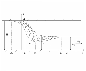
Consider a plane-parallel steady gravity current of an incompressible fluid inside a horizontally aligned rectangular duct. In the coordinate system shown in figure 1, the fluid depth $h(x)$ of this current satisfies the conditions

(2.1a,b)$$\begin{eqnarray}h(x)=H,\quad x\leqslant 0,\quad \text{and}\quad h(x)<H,\quad x>0,\end{eqnarray}$$

where $H$ is the duct height. Let us assume that the flow becomes uniform at a certain distance $a$ from the vertical section $x=0$ where the upper boundary of the fluid is deflected from the duct ceiling. The flow uniformity in these areas means that

(2.2a,b)$$\begin{eqnarray}\displaystyle h(x)=h_{2},\quad x\geqslant a,\quad \text{and}\quad \widetilde{p}(x)=p(x,h(x))=p_{1},\quad x\leqslant -a, & & \displaystyle\end{eqnarray}$$

(2.3)$$\begin{eqnarray}\displaystyle u(x,z)=\left\{\begin{array}{@{}ll@{}}v_{1}, & x\leqslant -a,\\ v_{2}, & x\geqslant a,\end{array}\right.\!\!\!\quad \text{and}\quad w(x,z)=0,\quad |x|\geqslant a. & & \displaystyle\end{eqnarray}$$

Here $p(x,z)$ and $\widetilde{p}(x)$ are the specific pressures in the fluid and on its surface; $u(x,z)$ is the horizontal velocity of the fluid directed along the $x$ axis; $w(x,z)$ is the vertical velocity of the fluid; and $h_{2}$, $p_{1}$, $v_{1}$ and $v_{2}$ are some given values.

Figure 1. Potential flow of an ideal incompressible fluid flowing from a horizontally aligned rectangular duct. The free fluid surface is the Benjamin solution (solid line 1) and the other solution is where the free surface of the fluid is deflected from the duct ceiling at a zero angle (dotted line 2).

We assume that the atmospheric pressure on the free surface of the fluid is equal to zero, i.e. $\widetilde{p}(x)=0$ at $x\geqslant 0$, and that the fluid surface $z=h(x)$ is a streamline with the horizontal velocity of the fluid at the stagnation point $\text{A}=(0,H)$ being

(2.4)$$\begin{eqnarray}u_{0}=u(0,H)=0.\end{eqnarray}$$

Benjamin (Reference Benjamin1968) showed that in this case, from the Bernoulli equation along the surface streamline (with allowance for the mass and momentum conservation laws on the segment $|x|\leqslant a$), it follows that the parameters of a piecewise-constant solution (2.2) and (2.3) are determined uniquely and are calculated by the following:

(2.5a-d)$$\begin{eqnarray}h_{2}=H/2,\quad v_{1}=c_{1}/2,\quad v_{2}=\sqrt{2}c_{2},\quad p_{1}=-c_{1}^{2}/8,\end{eqnarray}$$

where $c_{1}=\sqrt{gH}$ and $c_{2}=\sqrt{gh_{2}}$ are the velocities of propagation of small perturbations within the framework of the shallow-water theory and $g$ is the acceleration due to gravity. It follows from (2.5) that the flow is subcritical $(v_{1}<c_{1})$ in the domain $x\leqslant -a$ and supercritical $(v_{2}>c_{2})$ in the domain $x\geqslant a$.

3 One-parameter family of approximate solutions obtained within the framework of the model of an ideal incompressible fluid

Within the framework of the ideal incompressible fluid model, the plane-parallel steady flow is described by the continuity equation

(3.1)$$\begin{eqnarray}u_{x}+w_{z}=0\end{eqnarray}$$

and by the steady Euler equations

(3.2a,b)$$\begin{eqnarray}uu_{x}+wu_{z}+p_{x}=0,\quad uw_{x}+ww_{z}+p_{z}+g=0\end{eqnarray}$$

for the horizontal and vertical components of the fluid velocity. A consequence of equations (3.2) is the Bernoulli equation

(3.3)$$\begin{eqnarray}B={\displaystyle \frac{u^{2}+w^{2}}{2}}+gz+p=\text{const.}\end{eqnarray}$$

along each fluid streamline. For the potential flow $u_{z}-w_{x}=0$, the constant on the right-hand side of (3.3) is identical for all streamlines. From (3.1) and (3.2) follow the equations

(3.4a,b)$$\begin{eqnarray}\displaystyle (u^{2}+p)_{x}+(uw)_{z}=0,\quad (uw)_{x}+(w^{2}+p+gz)_{z}=0, & & \displaystyle\end{eqnarray}$$

which are conservation laws for the horizontal and vertical momenta of the fluid written in differential form.

First we will simulate the flow under consideration by the solution

(3.5a-d)$$\begin{eqnarray}u(x,z),\quad w(x,z),\quad p(x,z),\quad 0\leqslant z\leqslant h(x),\end{eqnarray}$$

of equations (3.1) and (3.2), satisfying the conditions (2.1) and the following boundary conditions at infinity:

(3.6a,b)$$\begin{eqnarray}\displaystyle \lim _{x\rightarrow +\infty }h(x)=h_{2},\quad \lim _{x\rightarrow -\infty }p(x,H)=p_{1}, & & \displaystyle\end{eqnarray}$$

(3.7a-c)$$\begin{eqnarray}\displaystyle \lim _{x\rightarrow -\infty }u(x,z)=v_{1},\quad \lim _{x\rightarrow +\infty }u(x,z)=v_{2},\quad \lim _{x\rightarrow \pm \infty }w(x,z)=0, & & \displaystyle\end{eqnarray}$$

which are consistent with the conditions (2.2) and (2.3). Assuming that the fluid surface $z=h(x)$ is the streamline in solution (3.5), we obtain the kinematic condition on this surface as

(3.8)$$\begin{eqnarray}w(x,h)=u(x,h)h_{x}.\end{eqnarray}$$

Let us integrate the differential equations (3.1) and (3.4a) with respect to $z$ from $0$ to $h$ and with respect to $x$ from $x_{1}$ to $x_{2}$. Taking into account the kinematic condition (3.8) and the no-normal-flow condition on the duct bottom,

(3.9)$$\begin{eqnarray}w(x,0)=0,\end{eqnarray}$$

we obtain on the spatial interval $[x_{1},x_{2}]$ the integral conservation laws for the mass and horizontal momentum of the fluid:

(3.10a,b)$$\begin{eqnarray}\left.\left(\int _{0}^{h}u\,\text{d}z\right)\right|_{x_{1}}^{x_{2}}=0,\quad \left.\left(\int _{0}^{h}(u^{2}+p)\,\text{d}z\right)\right|_{x_{1}}^{x_{2}}=\int _{x_{1}}^{x_{2}}\widetilde{p}h_{x}\,\text{d}x.\end{eqnarray}$$

Based on conditions (2.1), we have

(3.11a,b)$$\begin{eqnarray}h_{x}=0,\quad x<0,\quad \text{and}\quad \widetilde{p}=0,\quad x\geqslant 0;\end{eqnarray}$$

correspondingly, for our problem we obtain

(3.12)$$\begin{eqnarray}\int _{x_{1}}^{x_{2}}\widetilde{p}h_{x}\,\text{d}x=0.\end{eqnarray}$$

Let us assume that the solution (3.5) approximately satisfies conditions (2.2) and (2.3). In this case, the Bernoulli equation (3.3) written with respect to the surface streamline $z=h(x)$ yields the following approximate relation:

(3.13)$$\begin{eqnarray}v_{1}^{2}/2+gH+p_{1}=v_{2}^{2}/2+gh_{2}.\end{eqnarray}$$

As the pressure of the fluid in a uniform flow obeys the hydrostatic law,

$$\begin{eqnarray}p=\widetilde{p}+g(h-z)\quad \Rightarrow \quad \int _{0}^{h}p\,\text{d}z=\widetilde{p}h+gh^{2}/2,\end{eqnarray}$$

then the approximate expressions for solution (3.5), which follow from the conservation laws (3.10) at $x_{1}<-a$ and $x_{2}>a$, are

(3.14a,b)$$\begin{eqnarray}\displaystyle q=Hv_{1}=h_{2}v_{2},\quad Hv_{1}^{2}+gH^{2}/2+Hp_{1}=h_{2}v_{2}^{2}+gh_{2}^{2}/2, & & \displaystyle\end{eqnarray}$$

where $q$ is the flow rate of the fluid.

If pressure $p_{1}<0$, the system of equations (3.13) and (3.14) admit the one-parameter family of solutions

(3.15a-c)$$\begin{eqnarray}\displaystyle v_{1}={\displaystyle \frac{c_{1}h_{2}}{H}}=h_{2}\sqrt{{\displaystyle \frac{g}{H}}},\quad v_{2}=c_{1}=\sqrt{gH},\quad h_{2}=H-\sqrt{{\displaystyle \frac{2H|p_{1}|}{g}}}, & & \displaystyle\end{eqnarray}$$

in which the parameter is $p_{1}$. The depth positive condition $h_{2}>0$ leads to the following restriction on this parameter:

(3.16)$$\begin{eqnarray}-c_{1}^{2}/2<p_{1}<0.\end{eqnarray}$$

It follows from (3.15) that the flow is subcritical in the domain $x\leqslant -a$ and supercritical in the domain $x\geqslant a$ for all values of the pressure $p_{1}$ satisfying inequalities (3.16). In this case, the velocity $v_{2}$ does not depend on the value $p_{1}$, but the velocity $v_{1}$, depth $h_{2}$ and flow rate $q$ decrease monotonically to zero with $p$ decreasing to $-c_{1}^{2}/2$.

For the correctness of solution (3.15), the Bernoulli equation (3.3) has to be satisfied along the entire surface streamline $z=h(x)$, in particular, at the point $\text{A}=(0,H)$, where the surface pressure is $\widetilde{p}(0)=0$. From here, taking into account equations (3.13) and (3.14), we obtain

(3.17a,b)$$\begin{eqnarray}\displaystyle {\displaystyle \frac{u_{0}^{2}}{2}}={\displaystyle \frac{v_{1}^{2}}{2}}+p_{1}={\displaystyle \frac{gh_{2}^{2}}{2H}}+p_{1}={\displaystyle \frac{gH}{2}}-\sqrt{2gH|p_{1}|}\geqslant 0\quad \Rightarrow \quad |p_{1}|\leqslant {\displaystyle \frac{gH}{8}}.\quad & & \displaystyle\end{eqnarray}$$

As a result, at $u_{0}=0$ we obtain the Benjamin solution (2.5), and at $u_{0}>0$ we obtain a family of solutions whose parameters satisfy the inequalities

(3.18a,b)$$\begin{eqnarray}-c_{1}^{2}/8<p_{1}<0,\quad H/2<h_{2}<H,\quad c_{1}/2<v_{1}<c_{1}.\end{eqnarray}$$

Thus, the Benjamin solution is the limiting solution for the one-parameter family of solutions (3.15) and (3.18) that describe potential flows where the free surface of the fluid is deflected from the duct ceiling at a zero angle (dotted curve 2 in figure 1). Using the method proposed by Plotnikov & Toland (Reference Plotnikov and Toland2004), it can be shown that, within the framework of potential flows of an ideal fluid, the free surface of the liquid in the Benjamin solution (solid curve 1 in figure 1) is deflected from the duct ceiling at an angle of $60^{\circ }$.

4 Solutions that allow the formation of a vortex-flow region in the vicinity of the liquid separation point from the duct ceiling

We describe the flows that model the solutions (3.15) satisfying the condition

(4.1)$$\begin{eqnarray}-c_{1}^{2}/2<p_{1}<-c_{1}^{2}/8,\end{eqnarray}$$

which leads to a violation of the inequality (3.17a). For such solutions, the fluid surface $z=h(x)$ is not a single streamline on the interval $[-a,a]$. In this case the Bernoulli equation (3.3) used to derive (3.13) is not satisfied on the fluid surface $z=h(x)$ over the entire interval $[-a,a]$. Moreover, as the kinematic condition (3.8) is not satisfied on the entire interval $[-a,a]$, the integral conservation laws (3.10) for $x_{1}<-a$ and $x_{2}>a$ cannot be derived from the differential continuity and Euler equations (3.1) and (3.2). Thus, to describe such flows, the integral mass and momentum conservation laws (3.10) should be taken as the basic relations, which do not follow from the differential equations of the ideal incompressible fluid in the general case.

Under condition (4.1) a vortex-flow region is formed in the neighbourhood of the point $\text{A}=(0,H)$, where the fluid separates from the duct ceiling (figure 2). Let us assume that this region has the form

$$\begin{eqnarray}W_{1}=\{(x,z):b_{1}<x<b_{2},\unicode[STIX]{x1D707}(x)<z<h(x)\},\end{eqnarray}$$

where $-a<b_{1}<0$, $a>b_{2}>0$ and the function $z=\unicode[STIX]{x1D707}(x)$ satisfies the conditions

$$\begin{eqnarray}\unicode[STIX]{x1D707}(b_{1})=h(b_{1})=H,\quad \unicode[STIX]{x1D707}(b_{2})=h(b_{2})<H.\end{eqnarray}$$

We will also assume that the function $z=\unicode[STIX]{x1D707}(x)$ is part of the streamline

(4.2)$$\begin{eqnarray}z=\unicode[STIX]{x1D702}(x)=\left\{\begin{array}{@{}ll@{}}H, & x\leqslant b_{1},\\ \unicode[STIX]{x1D707}(x), & b_{1}\leqslant x\leqslant b_{2},\\ h(x), & x\geqslant b_{2},\end{array}\right.\end{eqnarray}$$

separating the vortex-flow region $W_{1}$ from the potential-flow region $W_{2}=W\setminus W_{1}$, where

$$\begin{eqnarray}W=\{(x,z):0\leqslant z\leqslant h(x,t)\}\end{eqnarray}$$

is the area of existence of the solution (3.5)–(3.7). This assumption allows to use the formula (3.13) obtained from Bernoulli equation (3.3) and formulae (3.14) obtained from the integral conservation laws (3.10) to construct solutions (3.15) in which the pressure $p_{1}$ satisfies the inequalities (4.1). The parameters of such solutions satisfy the conditions

$$\begin{eqnarray}-c_{1}^{2}/2<p_{1}<-c_{1}^{2}/8,\quad 0<h_{2}<H/2,\quad 0<v_{1}<c_{1}/2.\end{eqnarray}$$

If streamline (4.2) has discontinuous derivatives at the points $x=b_{i}$, i.e. satisfies the conditions

$$\begin{eqnarray}\lim _{x\rightarrow b_{1}+0}\unicode[STIX]{x1D707}^{\prime }(x)<0,\quad \lim _{x\rightarrow b_{2}-0}\unicode[STIX]{x1D707}^{\prime }(x)>h^{\prime }(b_{2}),\end{eqnarray}$$

then it follows from the continuity of the fluid velocity at these points that

(4.3a,b)$$\begin{eqnarray}u(b_{1},H)=w(b_{1},H)=0,\quad u(b_{2},h_{b})=w(b_{2},h_{b})=0,\quad h_{b}=h(b_{2}).\end{eqnarray}$$

Figure 2. The flows in which the vortex-flow region $W_{1}$ is formed in the vicinity of the point A.

Using the Bernoulli equation (3.3) written for streamline (4.2) at points with coordinates $(-\infty ,H)$, $(b_{1},H)$, $(b_{2},h_{b})$ and $(+\infty ,h_{2})$ taking into account conditions (3.6), (3.7) and (4.3) we have

(4.4)$$\begin{eqnarray}v_{1}^{2}/2+gH+p_{1}=gH+p_{b}=gh_{b}=v_{2}^{2}/2+gh_{2}.\end{eqnarray}$$

From here, with allowance for formulae (3.15), we obtain the surface pressure

$$\begin{eqnarray}p_{b}=\widetilde{p}(b_{1})=gH/2-\sqrt{2gH|p_{1}|}<0\end{eqnarray}$$

on the left boundary of the vortex-flow region $W_{1}$ and the depth

(4.5)$$\begin{eqnarray}h_{b}=h(b_{2})=3H/2-\sqrt{2H|p_{1}|/g}\end{eqnarray}$$

on the right boundary of this region. It follows from (3.15) and (4.5) that $h_{b}-h_{2}=H/2$ for any value of the pressure $p_{1}$ satisfying condition (4.1). In this case, the characteristic vertical size

$$\begin{eqnarray}H-h_{b}=\sqrt{2H|p_{1}|/g}-H/2\end{eqnarray}$$

of the domain $W_{1}$ increases from $0$ to $H/2$ as $p_{1}$ decreases from $-c_{1}^{2}/8$ to $-c_{1}^{2}/2$.

Note that the conditions (4.3) leading to equalities (4.4) provide the smallest possible size of the vortex-flow region $W_{1}$.

5 Solutions in which part of the uniform flow energy is converted into energy of the small-scale fluid motion

In the general case, the solutions (2.1)–(2.3) of the considered problem depend on two parameters, namely, pressure $p_{1}$ and velocity $v_{1}$, which determine the depth $h_{2}$ and velocity $v_{2}$ of the fluid flowing from the duct. In the one-parameter family of solutions (3.15) obtained under condition (3.16), the pressure $p_{1}$ and velocity $v_{1}$ are related by the following equality:

(5.1)$$\begin{eqnarray}v_{1}+\sqrt{2|p_{1}|}=c_{1}.\end{eqnarray}$$

Assume that equality (5.1) is not satisfied. Then, the system of equations (3.13) and (3.14) becomes incompatible. A similar situation arises for the shocks that model hydraulic bores in shallow-water theory (Stocker Reference Stocker1957). On such shocks, the system of mass and total momentum conservation laws is incompatible with the energy conservation law, which at standing shocks is equivalent to the local momentum conservation law; its analogue in our problem is equation (3.13). Moreover, the criterion for the shock stability (Friedrichs & Lax Reference Friedrichs and Lax1971; Lax Reference Lax1972) is energy inequality, due to which the energy decreases (is lost) when the fluid flows through the shock. For hydraulic bores, this means that part of the free-stream energy behind the bore front is transformed to the energy of small-scale fluid motion, which is not taken into account in the shallow-water theory.

We will apply this approach to construct energy-stable solutions (2.1)–(2.3) and (3.14), for which equality (5.1) does not hold. These solutions simulate flows in which the small-scale fluid motion occurs on the free surface of the liquid near the point of its separation from the duct ceiling. Figure 3 shows a case of surface wave breakdown in some interval $(a_{2},a_{3})$ that leads to the formation of surface turbulent-vortex flow in the same interval $(a_{1},a_{4})$. Such small-scale fluid perturbations drift mostly downstream, gradually damping (due to the action of viscous friction) on approaching the horizontal boundaries of this region. Herein, we will neglect friction at the bottom and ceiling of the duct. With this in mind, we assume that for $x<a_{1}$ and $x>a_{4}$ the flow becomes potential, and also that for $x<-a<a_{1}$ and for $x>a>a_{4}$ it becomes uniform, i.e. satisfy the conditions (2.2) and (2.3). Similar assumptions are typically made in the modelling of hydraulic bores in the framework of shallow-water theory (Stocker Reference Stocker1957).

Figure 3. Flows in which waves break down on the free surface of the liquid near the point A, which leads to the formation of a surface region of the turbulent-vortex flow.

Given these assumptions, the parameters of the considered flows in the interval $[x_{1},x_{2}]$, where $x_{1}<-a$ and $x_{2}>a$, satisfy the integral mass and total momentum conservation laws (3.10) from which, taking into account (2.1)–(2.3) and (3.12), we obtain equations (3.14). Excluding from these equations fluid velocities $v_{1}$ and $v_{2}$, we have

(5.2)$$\begin{eqnarray}{\displaystyle \frac{q^{2}}{Hh_{2}}}(H-h_{2})={\displaystyle \frac{g}{2}}(H^{2}-h_{2}^{2})+Hp_{1}.\end{eqnarray}$$

Since for $h_{2}<H$ the left side of this equation is positive, the right side must also be positive. From this we obtain the following restriction on the pressure:

(5.3)$$\begin{eqnarray}p_{1}>-{\displaystyle \frac{g}{2H}}(H^{2}-h_{2}^{2})=-{\displaystyle \frac{c_{1}^{2}}{2}}\left(1-{\displaystyle \frac{h_{2}^{2}}{H^{2}}}\right).\end{eqnarray}$$

A consequence of the system (3.1) and (3.2) is

(5.4)$$\begin{eqnarray}(uB)_{x}+(wB)_{y}=0,\end{eqnarray}$$

where $B$ is the Bernoulli function in (3.3). This equation is a differential form of the energy conservation law of a liquid. Integrating equation (5.4) taking into account the conditions (3.8), (3.9) and (3.11), we obtain the integral energy conservation law

(5.5)$$\begin{eqnarray}\left.\left(\int _{0}^{h}u\left({\displaystyle \frac{u^{2}+w^{2}}{2}}+gz+p\right)\text{d}z\right)\right|_{x_{1}}^{x_{2}}=0.\end{eqnarray}$$

When modelling the flows described in the previous section, this conservation law should be taken as the basic relation, which does not follow from the differential equations (3.1) and (3.2) in the general case. From the conservation law (5.5) at $x_{1}<-a$ and $x_{2}>a$, taking into account (2.2) and (2.3), we obtain

$$\begin{eqnarray}(q(v^{2}/2+gh+\widetilde{p}))|_{x_{1}}^{x_{2}}=0.\end{eqnarray}$$

For the stability of the solutions (2.1)–(2.3), (3.14) and (5.3), considered in this section, it is necessary to fulfill the energy inequality

$$\begin{eqnarray}(q(v^{2}/2+gh+\widetilde{p}))|_{x_{1}}^{x_{2}}<0,\end{eqnarray}$$

which (given the fact that $q=\text{const.}>0$) can be rewritten in the form

(5.6)$$\begin{eqnarray}v_{1}^{2}/2+gH+p_{1}>v_{2}^{2}/2+gh_{2}.\end{eqnarray}$$

Using formulae (3.14) and (5.2), we exclude from the inequality (5.6) the fluid velocities $v_{1}$ and $v_{2}$. As a result, we obtain the following restriction on the pressure:

$$\begin{eqnarray}p_{1}<-{\displaystyle \frac{g}{2H}}(H-h_{2})^{2}=-{\displaystyle \frac{c_{1}^{2}}{2}}\left(1-{\displaystyle \frac{h_{2}}{H}}\right)^{2}.\end{eqnarray}$$

Thus, under the condition

(5.7)$$\begin{eqnarray}-{\displaystyle \frac{c_{1}^{2}}{2}}\left(1-{\displaystyle \frac{h_{2}^{2}}{H^{2}}}\right)<p_{1}<-{\displaystyle \frac{c_{1}^{2}}{2}}\left(1-{\displaystyle \frac{h_{2}}{H}}\right)^{2},\end{eqnarray}$$

equations (3.14) define a two-parameter family of energy-stable solutions (2.1)–(2.3). Note that the method for constructing these solutions is similar to the method using the Kutta condition in aerodynamics (Clancy Reference Clancy1975).

The determination of the parameters of a particular solution (3.14) and (5.7) is conveniently carried out as follows. First set the depth $h_{2}\in (0,H)$, after which we select the pressure $p_{1}$ satisfying the inequalities (5.7). Next, from equation (5.2) we find the flow rate $q$, which we use to calculate the velocities $v_{1}=q/H$ and $v_{2}=q/h_{2}$. For example, if the depth $h_{2}=H/2$, as in the Benjamin solution (2.5), then the inequality (5.7) takes the form

(5.8)$$\begin{eqnarray}-3c_{1}^{2}/8<p_{1}<-c_{1}^{2}/4.\end{eqnarray}$$

Choosing $p_{1}$ in the middle of the interval (5.8) and using equation (5.2) we obtain

(5.9a-d)$$\begin{eqnarray}p_{1}=-{\displaystyle \frac{5c_{1}^{2}}{16}},\quad q={\displaystyle \frac{Hc_{1}}{4}},\quad v_{1}={\displaystyle \frac{c_{1}}{4}},\quad v_{2}={\displaystyle \frac{c_{1}}{2}}={\displaystyle \frac{c_{2}}{\sqrt{2}}}.\end{eqnarray}$$

It is interesting to note that, in contrast to the one-parameter family of solutions (3.15) and (3.16), to which the Benjamin solution (2.5) belongs, in the solution (5.9) the flow is subcritical, for both $x<-a$ and $x>a$.

6 Justification of the applicability of the constructed solutions on the basis of the local hydrostatic approximation

The classical method of justifying the applicability of vertically averaged solutions of equations of the ideal incompressible fluid is based on the long-wave approximation (Friedrichs Reference Friedrichs1948), which implies that the fluid flow is potential and the characteristic depth of the flow $H_{0}$ is much smaller than the characteristic length of the surface waves $L_{0}$, i.e. $\unicode[STIX]{x1D700}=H_{0}^{2}/L_{0}^{2}\ll 1$. For this reason (Stocker Reference Stocker1957), the spatial derivative of the depth $h$ of the plane-parallel flow satisfies the condition $|h_{x}|\leqslant O(\sqrt{\unicode[STIX]{x1D700}})$. However, in our case, this method is not applicable, since the flows studied in §§ 4 and 5 are not potential, and the potential flows considered in § 3 satisfy the condition $|h_{x}|\leqslant 1$ for all $x>0$ only if $(H-h_{2})/H\leqslant 1$. Therefore, to justify the applicability of the approximate solutions (2.1)–(2.3) constructed in this paper, we apply the local hydrostatic approximation proposed by Ostapenko (Reference Ostapenko2018).

We will say that when the fluid flows out from a rectangular duct (figure 1) its parameters satisfy the local hydrostatic approximation at the point $(x,z)$, if the inequality $w^{2}(x,z)/c_{1}^{2}<\unicode[STIX]{x1D6FF}\ll 1$ is satisfied at this point, where $\unicode[STIX]{x1D6FF}$ is a given small number. Let us divide the domain $V$ of existence of the two-dimensional flow under consideration into two subdomains:

$$\begin{eqnarray}V_{1}(\unicode[STIX]{x1D6FF})=\{(x,z)\in V:w^{2}(x,z)/c_{1}^{2}<\unicode[STIX]{x1D6FF}\},\quad V_{2}(\unicode[STIX]{x1D6FF})=V\setminus V_{1}(\unicode[STIX]{x1D6FF}).\end{eqnarray}$$

In the domain $V_{1}$, we introduce dimensionless variables

(6.1a-f)$$\begin{eqnarray}x_{\ast }=\frac{\sqrt{\unicode[STIX]{x1D6FF}}}{H}x,\quad z_{\ast }=\frac{z}{H},\quad h_{\ast }=\frac{h}{H},\quad u_{\ast }=\frac{u}{c_{1}},\quad w_{\ast }=\frac{w}{\sqrt{\unicode[STIX]{x1D6FF}}c_{1}},\quad p_{\ast }=\frac{p}{c_{1}^{2}},\end{eqnarray}$$

which, after the substitution $\unicode[STIX]{x1D6FF}=H_{0}^{2}/L_{0}^{2}$, $H_{0}=H$, transform into the dimensionless variables of the long-wave approximation, where the variable $L_{0}$ can be considered as the characteristic wavelength along the streamlines passing inside the domain $W_{1}(\unicode[STIX]{x1D6FF})$.

We will assume that the domain $V_{2}(\unicode[STIX]{x1D6FF})$ in which the local hydrostatic approximation is not satisfied is bounded. With this in mind, the number $a$ included in (2.2) and (2.3) is chosen so that for $|x|>a$ the flow is potential and condition $|x|<a$ is satisfied for all points $(x,z)\in V_{2}(\unicode[STIX]{x1D6FF})$. In this case, the flows considered in §§ 3 and 4 are described by the integral mass, momentum and energy conservation laws (3.10) and (5.5), in which $x_{1}<-a$ and $x_{2}>a$. Writing down these conservation laws in dimensionless variables (6.1), by analogy with Ostapenko (Reference Ostapenko2018), we obtain the relations

(6.2a-c)$$\begin{eqnarray}\displaystyle q|_{x_{1}}^{x_{2}}=0,\quad (qv+h^{2}/2+h\widetilde{p})|_{x_{1}}^{x_{2}}=0,\quad (v^{2}/2+h+\widetilde{p})|_{x_{1}}^{x_{2}}=0, & & \displaystyle\end{eqnarray}$$

with accuracy no less than $O(\unicode[STIX]{x1D6FF})$. In equations (6.2) the asterisk is omitted for brevity. For the flows studied in § 5, equation (6.2c) should be replaced by the energy inequality

(6.3)$$\begin{eqnarray}(v^{2}/2+h+\widetilde{p})|_{x_{1}}^{x_{2}}<0.\end{eqnarray}$$

Given that acceleration $g=1$ in dimensionless variables (6.1), the relations (6.2) imply formulae (3.13) and (3.14) and relations (6.2a,b) along with inequality (6.3) imply formula (5.2) and inequality (5.7). It follows that the approximate piecewise-constant solutions (2.1)–(2.3) that we have constructed in §§ 3–5 transmit the parameters of the considered flows with accuracy no less than $O(\unicode[STIX]{x1D6FF})$.