


1. Introduction
The controllable production of microdroplets and microfibres from thin liquid jets is of great interest in various scientific and engineering applications, such as medicine, pharmaceuticals, material science, chemistry, food, agriculture, textile, etc. (Gañán-Calvo et al. Reference Gañán-Calvo, Montanero, Martín-Banderas and Flores-Mosquera2013). Capillary flows have been used to produce micro-jets effectively (Barrero & Loscertales Reference Barrero and Loscertales2007), where the interfaces of different fluid jets can be smoothly stretched to of the order of microns or less under the action of an external force field. As type of capillary flow, based on the flow focusing (FF) technique was proposed by Gañán-Calvo (Reference Gañán-Calvo1998), where a steady microscopic liquid jet is formed under the driving of an external high-speed co-flowing gas stream. FF has the advantage of producing a micron-level monodisperse spray, and has become a popular method of producing sub-millimetre jets through hydrodynamic means (Montanero & Gañán-Calvo Reference Montanero and Gañán-Calvo2020).
The research on the phenomenon of a liquid jet breaking into droplets has a history of more than a century since the pioneering work of Rayleigh (Reference Rayleigh1878), where a temporal instability analysis of an inviscid liquid cylinder flowing with a uniform velocity was performed. The influence of the surrounding gas was neglected and surface tension was the only destabilizing factor. When the jet velocity is relatively small, Rayleigh's results are consistent with experiments, while for higher jet velocities, Rayleigh's results deviate from experiments. Weber (Reference Weber1931) found that the liquid viscosity has stabilizing effects, reducing the breakup rate and increasing the droplet size. Chandrasekhar (Reference Chandrasekhar1961) proved that the mechanism of Rayleigh jet instability is capillary pinching. In the Rayleigh instability theory, the predicted droplet sizes are of the same order as the jet diameter. However, this theory cannot be applied to the atomization phenomenon which is the breakup of a liquid jet into droplets much smaller than the jet diameter. To explain the atomization process, Taylor (Reference Taylor1962) took the gas density into account. He considered the limiting case of an infinitely thick jet and extremely small gas-to-liquid density ratio. Lin & Chen (Reference Lin and Chen1998) investigated the role of interfacial shear in the onset of instability of a cylindrical viscous liquid jet in a viscous gas surrounded by a coaxial circular pipe. They reported that the mechanism of the jet atomization is the shear and pressure fluctuation at the interface.
The instability and mode transition in FF have attracted more and more attention (Herrada et al. Reference Herrada, Montanero, Ferrera and Gañán-Calvo2010; Guerrero et al. Reference Guerrero, Chang, Fragkopoulos and Fernandez-Nieves2020; Mu et al. Reference Mu, Qiao, Si, Cheng and Ding2021). Rosell-Llompart & Gañán-Calvo (Reference Rosell-Llompart and Gañán-Calvo2008) distinguished two flow regimes in FF, which depend on the interaction between the liquid jet and the co-flowing gas stream (e.g. the Weber number  ${\textit {We}}$). For
  $1 < {\textit {We}} < 20$, it is ‘capillary FF’, while for
  ${\textit {We}} > 20$, it turns into ‘turbulent FF’. Gordillo, Pérez-Saborid & Gañán-Calvo (Reference Gordillo, Pérez-Saborid and Gañán-Calvo2001) performed a linear temporal instability analysis of an inviscid jet and the co-flowing gas stream surrounding the jet, where the influences of the basic-velocity profiles of the liquid and gas are considered by solving the Navier–Stokes equations with the slenderness approximation. Their analysis in the case of a uniform liquid velocity profile recovered the classical Rayleigh inviscid result for well-developed and very thin gas boundary layers, but more importantly, the consideration of realistic liquid velocity profiles (i.e. non-uniform velocity profiles) revealed new families of modes which are essential to explain atomization experiments at large enough Weber numbers, and do not appear in the classical stability analysis of inviscid parallel streams.
It should be emphasized that many practical applications involve non-Newtonian viscoelastic jets, such as inkjet printing, micro/nano-fibre manufacture, spinning and electrospinning of polymeric solutions (Eggers & Villermaux Reference Eggers and Villermaux2008; Basaran, Gao & Bhat Reference Basaran, Gao and Bhat2013; Alsharif, Uddin & Afzaal Reference Alsharif, Uddin and Afzaal2015; Li et al. Reference Li, Ke, Yin and Yin2019). The introduction of fluid elasticity can fundamentally modify the Newtonian flow dynamics. For example, the elasticity of fluid in high molecular polymer solutions may alter the linear amplification of disturbances in shear flows, shift the onset of laminar-to-turbulence transition and reduce drag in the turbulent flow regime (Page & Zaki Reference Page and Zaki2016). In past decades, the instability of viscoelastic jets has received widespread attention (Montanero & Gañán-Calvo Reference Montanero and Gañán-Calvo2008; Ponce-Torres et al. Reference Ponce-Torres, Montanero, Vega and Gañán-Calvo2016; Ye, Yang & Fu Reference Ye, Yang and Fu2016; Eggers, Herrada & Snoeijer Reference Eggers, Herrada and Snoeijer2020). However, in contrast to the large body of literature available on the study of Newtonian liquid jets, the theoretical work on the instability of viscoelastic jets is relatively limited due to the mathematical complexity in dealing with nonlinear rheological constitutive equations. Incipient research (e.g. Middleman Reference Middleman1965; Kroesser & Middleman Reference Kroesser and Middleman1969) that directly applied the linear stability theory to predict the axisymmetric breakup of viscoelastic jets did not achieve the same success as that with Newtonian fluid jets (Goldin et al. Reference Goldin, Yerushalmi, Pfeffer and Shinnar1969; Gordon, Yerushalmi & Shinnar Reference Gordon, Yerushalmi and Shinnar1973). The linearized instability analysis predicted that a viscoelastic jet exhibits more rapid growth of axisymmetric wave disturbances than its Newtonian counterpart, implying that elasticity is a purely destabilizing factor for all unstable disturbances (Goldin et al. Reference Goldin, Yerushalmi, Pfeffer and Shinnar1969; Liu & Liu Reference Liu and Liu2006, Reference Liu and Liu2008). This result does not agree with most experiments because viscoelastic jets generally take a longer time to break up into droplets than Newtonian ones (Gordon et al. Reference Gordon, Yerushalmi and Shinnar1973; Eggers & Villermaux Reference Eggers and Villermaux2008). In order to resolve this discrepancy between theoretical analysis and experimental observations, Goren & Gottlieb (Reference Goren and Gottlieb1982) proposed that the liquid may be subject to an unrelaxed axial tension due to its prior history. Under the assumption that the stress relaxation time constant is sufficiently large, Goren & Gottlieb (Reference Goren and Gottlieb1982) showed that the unrelaxed axial elastic tension can be a significant stabilizing influence.
However, there are some inherent limitations in Goren & Gottlieb's theory. First of all, the unrelaxed axial elastic tension is artificially specified (Ruo et al. Reference Ruo, Chen, Chung and Chang2011; Mohamed et al. Reference Mohamed, Herrada, Gañán-Calvo and Montanero2015; Xie et al. Reference Xie, Yang, Fu and Qin2016), and its real physical meaning is unclear. Secondly, the elastic tension decays exponentially with an increase in the distance from the nozzle. In order to maintain an approximate constant elastic tension, some constraints need to be imposed. For example, the validity of this assumption requires that the distance over which the velocity profile relaxes completely from the nozzle is much shorter than the distance corresponding to the elastic stress relaxation (Ruo et al. Reference Ruo, Chen, Chung and Chang2011). In the present study, we try to clarify the physical meaning of the unrelaxed elastic tension and remove unnecessary constraints through comprehensive and detailed investigation.
It is generally believed that when linear stability theory is used to study the mechanism of jet breakup, two primary conditions need to be satisfied to get results consistent with experiments: one is that the model must include all important parameters, such as viscosity, density, surface tension, etc.; the other is that the basic flow should be the same as or similar to the real flow. In specific research of FF, when the physical model is close to the actual situation, temporal stability analysis often gives results comparable to experiments (Si et al. Reference Si, Li, Yin and Yin2009). In the linear stability analysis of co-flowing liquid–gas jets performed by Gordillo et al. (Reference Gordillo, Pérez-Saborid and Gañán-Calvo2001), the consideration of realistic (non-uniform) basic velocity profiles revealed new families of modes which are essential to explain atomization experiments at large enough Weber numbers. We are surprised to see that almost all the previous studies adopted uniform velocity profiles in the linear stability analysis of viscoelastic jets, probably for the sake of mathematical simplicity. In this work, the temporal linear instability analysis is performed by considering viscoelastic jets with non-uniform basic-velocity profiles in the FF flow configuration. The liquid is assumed to be an Oldroyd-B viscoelastic fluid, which was commonly used in previous studies. The characteristic of an Oldroyd-B fluid is that its viscosity is independent of shear in flow and elastic effects can be clearly distinguished from the viscous effects. It has turned out to be an appropriate model in describing the viscoelasticity of dilute polymer solutions under small or moderate deformation (Larson Reference Larson1992; Morozov & van Saarloos Reference Morozov and van Saarloos2007; James Reference James2009).
The paper is organized as follows. Section 2 provides the governing equations for viscoelastic jets, the base-state velocity profile and stress tensor and the validation of the numerical method used in this study. In § 3, an energy budget analysis is implemented to access the dominating forces in the instability analysis of viscoelastic jets. In § 4, the influence of fluid elasticity on the jet instability is discussed in detail in § 4.1, where three different instability mechanisms can be identified by means of the energy budget analysis. Section 4.2 demonstrates the general features of instability modes by examining the variations of the maximum growth rate and the corresponding phase speed. In § 4.3, we investigate the transitions of instability modes in parameter spaces and provide the transition boundaries between different modes. Finally, the study is summarized and concluded in § 5.
2. Theoretical model and numerical method
2.1. Governing equations
Consider the linear instability of an incompressible viscoelastic liquid jet of radius  $R_{1}$ and density
  $\rho _{1}$. The jet is surrounded by a viscous gas in an external environment, and the gas stream is considered as a cylinder of radius
  $R_{2}$ with the outside surface being assumed to slip. The effects of gravity and temperature are negligible. Only the axisymmetric disturbance is considered. The theoretical model is sketched in figure 1, where a cylindrical polar coordinate system is used with
  $r$,
$r$,  $\theta$ and
  $z$ denoting the radial, azimuthal and axial directions. The characteristic scales used for non-dimensionalizing the governing equations are: radius
  $R_{1}$ for lengths, base-flow velocity
  $U_{0}$ at the centre for velocities,
  $R_{1} / U_{0}$ for time and
  $\rho _{1} U_{0}^{2}$ for pressures and stresses.

Figure 1. Schematic diagram of the theoretical model of viscoelastic jets.
The dimensionless continuity and Cauchy momentum equations for the viscoelastic liquid are given by
 \begin{equation} \boldsymbol{\nabla} \boldsymbol{\cdot} \boldsymbol{V}_{1}=0,\quad \frac{\partial \boldsymbol{V}_{1}}{\partial t}+ \left(\boldsymbol{V}_{1} \boldsymbol{\cdot} \boldsymbol{\nabla}\right) \boldsymbol{V}_{1}={-}\boldsymbol{\nabla} p_1+\boldsymbol{\nabla} \boldsymbol{\cdot} \boldsymbol{T}. \end{equation}
Here,  $\boldsymbol {V}_{1}=v_{1} \boldsymbol {e}_{r}+w_{1} \boldsymbol {e}_{\!\theta }+u_{1} \boldsymbol {e}_{\!z}$ is the velocity field,
  $p_1$ is the pressure field and
  $\boldsymbol {T}$ is the deviatoric stress tensor, which can be decomposed into a polymer contribution
  $\boldsymbol {T}_{\!p}$ and a Newtonian solvent contribution
  $\boldsymbol {T}_{\!s}$, i.e.
  $\boldsymbol {T}=\boldsymbol {T}_{\!s}+\boldsymbol {T}_{\!p}$. The total viscosity of the solution is the sum of the solvent and polymer contributions, i.e.
  $\mu _{1}=\mu _{\!s}+\mu _{\!p}$, with
  $\mu _{\!s}$ and
  $\mu _{\!p}$ being the solvent and polymer viscosities, respectively. The solvent to solution viscosity ratio is denoted by
  $X=\mu _{\!s} / \mu _{1} ; X=1$ recovers the Newtonian limit. The dimensionless constitutive equation for the Newtonian solvent stress
  $\boldsymbol {T}_{\!s}$ is
 \begin{equation} \boldsymbol{T}_{\!s}=\frac{X}{{\textit{Re}}}\left[\boldsymbol{\nabla} \boldsymbol{V}_{1}+ \left(\boldsymbol{\nabla} \boldsymbol{V}_{1}\right)^{\mathrm{T}}\right], \end{equation}
while the polymer stress satisfies the Oldroyd-B constitutive relation (Bird, Armstrong & Hassager Reference Bird, Armstrong and Hassager1987; Larson Reference Larson1988)
 \begin{equation} \boldsymbol{T}_{\!p}+{\textit{Wi}} \overset{\triangledown}{{\boldsymbol{T}}}_{\!p} =\frac{1-X}{{\textit{Re}}}\left[\boldsymbol{\nabla} \boldsymbol{V}_{1}+\left(\boldsymbol{\nabla} \boldsymbol{V}_{1}\right)^{\mathrm{T}}\right], \end{equation}
where the superscripts  $\mathrm {T}$ and
  $\boldsymbol {\nabla }$ denote transpose and the upper-convected derivative defined by
 \begin{equation} \overset{\triangledown}{{\boldsymbol{T}}}_{\!p}= \frac{\partial \boldsymbol{T}_{\!p}}{\partial t}+\boldsymbol{V}_{1} \boldsymbol{\cdot} \boldsymbol{\nabla} \boldsymbol{T}_{\!p}-\left(\boldsymbol{\nabla} \boldsymbol{V}_{1}\right)^{\mathrm{T}} \boldsymbol{\cdot}\boldsymbol{T}_{\!p}-\boldsymbol{T}_{\!p} \boldsymbol{\cdot}\boldsymbol{\nabla} \boldsymbol{V}_{1}. \end{equation}
 For a fixed  $X$, the dimensionless groups relevant to the stability of the Oldroyd-B fluid are the Reynolds number
  ${\textit {Re}}=\rho _{1} U_{0} R_{1} / \mu _{1}$, the Weber number
  ${\textit {We}}=\rho _{1} U_{0}^{2} R_{1} / \sigma$, representing the ratio of inertial force to surface tension
  $(\sigma )$, and the Weissenberg number
  ${\textit {Wi}}=\lambda U_{0} / R_{1}$, which is the ratio of the polymer relaxation time
  $\lambda$ to the flow time scale. Alternatively, the elasticity number,
  ${\textit {El}} = {\textit {Wi}} / {\textit {Re}} =\lambda \mu _{1} / \rho _{1} R_{1}^{2}$, can be introduced, which represents the ratio of the elastic and viscous time scales of the liquid jet (Brenn, Liu & Durst Reference Brenn, Liu and Durst2000). The advantage of
  ${\textit {El}}$ is that its value is determined by the physical properties of the fluid itself and has nothing to do with the velocity. Obviously, when
  ${\textit {El}}=0$ (or equivalently
  ${\textit {Wi}}=0$), the model degenerates to the Newtonian fluid. On the other hand, if all nonlinear terms in (2.4) disappear, the Jeffreys constitutive relation (a linear viscoelastic model) is obtained as follows:
 \begin{equation} \boldsymbol{T}_{\!p}+{\textit{Wi}} \frac{\partial \boldsymbol{T}_{\!p}}{\partial t}= \frac{1-X}{{\textit{Re}}}\left[\boldsymbol{\nabla} \boldsymbol{V}_{1}+\left(\boldsymbol{\nabla} \boldsymbol{V}_{1}\right)^{\mathrm{T}}\right]. \end{equation}
To facilitate expression of the nonlinear terms in the constitutive equation, we define an operation
 \begin{equation} \left\langle\boldsymbol{T}_{\!p}, \boldsymbol{V}_{1}\right\rangle \equiv \boldsymbol{V}_{1} \boldsymbol{\cdot} \boldsymbol{\nabla} \boldsymbol{T}_{\!p}-\left(\boldsymbol{\nabla} \boldsymbol{V}_{1}\right)^{\mathrm{T}} \boldsymbol{\cdot} \boldsymbol{T}_{\!p}-\boldsymbol{T}_{\!p} \boldsymbol{\cdot} \boldsymbol{\nabla} \boldsymbol{V}_{1}, \end{equation}
which is bilinear and represents the coupling interaction between the polymer stress and the velocity. Using this notation, the upper-convected derivative can be rewritten as
 \begin{equation} \overset{\triangledown}{{\boldsymbol{T}}}_{\!p}=\frac{\partial \boldsymbol{T}_{\!p}}{\partial t}+ \left\langle\boldsymbol{T}_{\!p}, \boldsymbol{V}_{1}\right\rangle. \end{equation}
 The dimensionless governing equations for the ambient gas with density  $\rho _{2}$ and viscosity
  $\mu _{2}$ are given by
 \begin{equation} \boldsymbol{\nabla} \boldsymbol{\cdot} \boldsymbol{V}_{2}=0, \quad \frac{\partial \boldsymbol{V}_{2}}{\partial t}+\left(\boldsymbol{V}_{2} \boldsymbol{\cdot} \boldsymbol{\nabla}\right) \boldsymbol{V}_{2}={-}\frac{1}{Q} \boldsymbol{\nabla} p_{2}+\frac{N}{Q} \frac{1}{{\textit{Re}}} \nabla^{2} \boldsymbol{V}_{2}, \end{equation}
where  $\boldsymbol {V}_{2}=v_{2} \boldsymbol {e}_{r}+w_{2} \boldsymbol {e}_{\!\theta }+u_{2} \boldsymbol {e}_{\!z}$ is the velocity field,
  $p_{2}$ is the pressure field,
  $Q=\rho _{2} / \rho _{1}$ and
  $N=$
$N=$  $\mu _{2} / \mu _{1}$ are the density ratio and the viscosity ratio, respectively.
To close the system, consistent conditions at the symmetry axis  $r=0$ and the outside boundary
  $r=a$ with
  $a=R_{2} / R_{1}$ are needed
 \begin{equation} \left.\begin{gathered} v_1=\frac{\partial u_1}{\partial r}=\frac{\partial p_1}{\partial r}=0, \quad \mbox{at}\ r=0, \\ v_2=\frac{\partial u_2}{\partial r}=\frac{\partial p_2}{\partial r}=0, \quad \mbox{at}\ r=a. \end{gathered}\right\} \end{equation}
At the liquid–gas interface  $r=h(z, t)$, the continuity of velocity, and the kinematic and dynamic conditions are satisfied, i.e.
 $$\begin{gather} \boldsymbol{V}_{1} = \boldsymbol{V}_{2}, \end{gather}$$
 $$\begin{gather}v_{1} = \left(\frac{\partial}{\partial t}+\boldsymbol{V}_{1} \boldsymbol{\cdot} \boldsymbol{\nabla}\right) h, \end{gather}$$
 $$\begin{gather}(\boldsymbol{T}_{2} - \boldsymbol{T}_{1} ) \boldsymbol{\cdot} \boldsymbol{n} = \frac{1}{{\textit{We}}} \left( \boldsymbol{\nabla} \boldsymbol{\cdot} \boldsymbol{n}\right) \boldsymbol{n}, \end{gather}$$
where  $\boldsymbol {T}_{\!1}=-p_{1} \boldsymbol {I} + \boldsymbol {T}_{\!s}+\boldsymbol {T}_{\!p}$ and
  $\boldsymbol {T}_{\!2}=-p_{2} \boldsymbol {I} + N / {\textit {Re}} [\boldsymbol {\nabla } \boldsymbol {V}_{2}+(\boldsymbol {\nabla } \boldsymbol {V}_{2})^{\mathrm {T}}]$ with
  $\boldsymbol {I}$ the unit tensor and where
  $\boldsymbol {n}$ is the outward unit vector normal to the interface.
2.2. Basic-velocity profile and stress tensor
The first step in performing the stability analysis is to find the basic velocity profiles for the liquid and gas streams. In order to get reasonable results, the basic flow should be the same as or similar to the real flow, as stated in the introduction section. Lin & Ibrahim (Reference Lin and Ibrahim1990) derived an analytical velocity profile satisfying the Navier–Stokes equations in their study on the instability of a cylindrical Newtonian fluid jet encapsulated by a viscous gas in a vertical circular pipe. Gordillo et al. (Reference Gordillo, Pérez-Saborid and Gañán-Calvo2001) obtained the velocity profiles in the FF jet problem by numerically solving the boundary-layer equations. For given initial velocity profiles of liquid and gas, the evolution of the liquid and gas streams in space can be computed. However, the algebraic operation is complicated. On the other hand, several approximate velocity profiles have been successfully applied in theoretical analysis compared with the experimental results, e.g. that of the error function (Yecko, Zaleski & Fullana Reference Yecko, Zaleski and Fullana2002) and that of the hyperbolic–tangent function (Sevilla, Gordillo & Martínez-Bazán Reference Sevilla, Gordillo and Martínez-Bazán2002; Gañán-Calvo & Riesco-Chueca Reference Gañán-Calvo and Riesco-Chueca2006; Si et al. Reference Si, Li, Yin and Yin2009). In this work, velocity profiles of the hyperbolic–tangent function in the two fluids are utilized. The basic velocity is assumed to be axisymmetric and unidirectional, and denoted by  $\boldsymbol {U}_{i}=[0,0, U_{i}(r)]$, where the subscripts
  $i=1,2$ stand for the liquid and the gas, respectively.
The dimensionless form  $U_{i}(r)$, similar to that of Si et al. (Reference Si, Li, Yin and Yin2009), is selected as
 \begin{equation} U_{i}(r)=a_{i} \tanh \left(b_{i}(r-1)\right)+d_{i}, \end{equation}
where  $a_{i}, b_{i}$ and
  $d_{i} (i=1,2)$ are the coefficients to be determined. Using the following constraint conditions: (i) continuity of the velocity and shear stress at the jet interface; (ii) symmetry of the velocity at the symmetric axis; (iii) uniformity of the velocity at the outside boundary, the basic velocities can be written as (Si et al. Reference Si, Li, Yin and Yin2009)
 $$\begin{gather} U_{1}(r) = \left(U_{s}-1\right) \tanh \left[\frac{K}{U_{s}-1}(r-1)\right]+U_{s}, \end{gather}$$
 $$\begin{gather}U_{2}(r) = \left(U_{a}-U_{s}\right) \tanh \left[\frac{K}{N\left(U_{a}-U_{s}\right)}(r-1)\right]+U_{s}, \end{gather}$$
where  $U_{s}$ is the velocity at the unperturbed interface
  $(r=1), U_{a}$ is the velocity at the outside boundary
  $(r=a)$ and
  $K$ is the slope of the liquid velocity profile at the interface. The parameter
  $K$ characterizes the strength of interfacial shear. A large value of
  $K$ implies a strong interfacial shear. When
  $K=0$, one can get a uniform velocity profile in the whole flow field. In FF, the gas-to-liquid momentum ratio is very close to unity, and thus
  $U_{a} \approx Q^{-1 / 2}$ (see Si et al. Reference Si, Li, Yin and Yin2009), which is also used in this work.
Under the assumption of a steady-state axisymmetric and non-uniform basic velocity, the polymer contribution to the stress tensor in the base state can be obtained by solving (2.3) and (2.4), as follows:
 \begin{equation} \boldsymbol{\varGamma}=\left[\begin{array}{@{}ccc@{}} \varGamma_{r r} & 0 & \varGamma_{r z} \\ 0 & \varGamma_{\theta\! \theta} & 0 \\ \varGamma_{z r} & 0 & \varGamma_{z z} \end{array}\right]=\frac{1-X}{{\textit{Re}}}\left[\begin{array}{@{}ccc@{}} 0 & 0 & U_{1}^{\prime} \\ 0 & 0 & 0 \\ U_{1}^{\prime} & 0 & 2 {\textit{Wi}} U_{1}^{\prime 2} \end{array}\right], \end{equation}
where  $f^{\prime } \equiv {\mathrm {d} f}/{\mathrm {d} r}$. Note that there is a non-zero tension
  $\varGamma _{zz}$ along the streamlines proportional to the square of the velocity gradient, which does not appear for both Newtonian and linear viscoelastic models (i.e. the Jeffreys model). Thus, unlike the Newtonian and Jeffreys counterparts, the Oldroyd-B fluid exhibits a non-zero first normal stress difference
  $(\varGamma _{z z}-\varGamma _{r r})$. Most notably,
  $\varGamma _{z z}$ plays the role of unrelaxed axial elastic tension, compared with Goren & Gottlieb's theory, but the source of unrelaxed elastic tension is completely different. In Goren & Gottlieb's theory, the axial elastic tension was obtained by integrating (2.3) and (2.4) based on a uniform basic velocity
  $U$, i.e.
  $\bar {\tau }_{z z}(z)=$
  $\bar {\tau }_{a} \exp (-z / \lambda U)$ (see (2.6) in Ruo et al. Reference Ruo, Chen, Chung and Chang2011), where
  $\bar {\tau }_{a}$ is the axial tension at the nozzle exit and its magnitude needs to be specified artificially. In addition, Goren & Gottlieb's theory requires
  $\lambda U / l \gg 1$, with
  $l$ being the wavelength of a disturbance, so that the mathematical terms involving the spatial gradient of the tension can be negligible over distances comparable to the characteristic wavelength (Ruo et al. Reference Ruo, Chen, Chung and Chang2011). As a contrast, by using a non-uniform basic velocity, we get the axial elastic tension
  $\varGamma _{z z}=2(1-X) {\textit {El}}\, U_{1}^{\prime 2}$, which is a function of
  $r$ and related to the velocity gradient, elasticity number and solvent viscosity ratio. Note that no additional assumptions need to be introduced in our situation and the physical meaning of unrelaxed elastic tension is clear. A comparison of our result with Goren & Gottlieb's theory is summarized in table 1.
Table 1. Comparison of our result with Goren & Gottlieb's theory.

2.3. Linear stability analysis
To carry out the linear stability analysis, the base state is subjected to small amplitude axisymmetric disturbances as follows:
 $$\begin{gather} \boldsymbol{V}_{i} = \boldsymbol{U}_{i}+\tilde{\boldsymbol{V}}_{i}, \end{gather}$$
 $$\begin{gather}p_{i} = P_{i}+\tilde{p}_{i}, \end{gather}$$
 $$\begin{gather}\boldsymbol{T}_{\!p} = \boldsymbol{\varGamma}+\tilde{\boldsymbol{T}}_{\!p}. \end{gather}$$
For axisymmetric disturbances, the perturbation velocity and elastic stress tensor are
 \begin{equation} \tilde{\boldsymbol{V}}_{i}=\left[\begin{array}{@{}c@{}} \tilde{v}_{i} \\ 0 \\ \tilde{u}_{i} \end{array}\right] \quad \text{and}\quad \tilde{\boldsymbol{T}}_{\!p}=\left[\begin{array}{@{}ccc@{}} \tilde{\tau}_{r r} & 0 & \tilde{\tau}_{r z} \\ 0 & \tilde{\tau}_{\theta\! \theta} & 0 \\ \tilde{\tau}_{z r} & 0 & \tilde{\tau}_{z z} \end{array}\right], \end{equation}
respectively. It is worth noting that, although axisymmetric disturbances are considered, the inclusion of the component  $\tilde {\tau }_{\theta \!\theta }$ in the elastic stress tensor is necessary because the constitutive equation of
  $\tilde {\tau }_{\theta \!\theta }$ is related to the perturbation velocity
  $\tilde {v}_{1}$, which is non-zero (see (A2) and (A6) in Appendix A).
Substituting (2.14) into the governing equations (2.1a,b)–(2.3) and (2.8a,b) and neglecting high-order terms, we obtain the governing equations for disturbances as follows:
 $$\begin{gather} \boldsymbol{\nabla} \boldsymbol{\cdot} \tilde{\boldsymbol{V}}_{1}=0, \end{gather}$$
 $$\begin{gather}\frac{\partial \tilde{\boldsymbol{V}}_{1}}{\partial t}+\left(\tilde{\boldsymbol{V}}_{1} \boldsymbol{\cdot} \boldsymbol{\nabla}\right) \boldsymbol{U}_{1}+\left(\boldsymbol{U}_{1} \boldsymbol{\cdot} \boldsymbol{\nabla}\right) \tilde{\boldsymbol{V}}_{1}={-}\boldsymbol{\nabla} \tilde{p}_{1}+\boldsymbol{\nabla} \boldsymbol{\cdot} \tilde{\boldsymbol{T}}_{\!s}+\boldsymbol{\nabla} \boldsymbol{\cdot} \tilde{\boldsymbol{T}}_{\!p}, \end{gather}$$
 $$\begin{gather}\tilde{\boldsymbol{T}}_{\!s}=\frac{X}{{\textit{Re}}}\left[\boldsymbol{\nabla} \tilde{\boldsymbol{V}}_{1}+\left(\boldsymbol{\nabla} \tilde{\boldsymbol{V}}_{1}\right)^{\mathrm{T}}\right], \end{gather}$$
 $$\begin{gather}\tilde{\boldsymbol{T}}_{\!p}+{\textit{Wi}}\left[\frac{\partial \tilde{\boldsymbol{T}}_{\!p}}{\partial t}+\left\langle\tilde{\boldsymbol{T}}_{\!p}, \boldsymbol{U}_{1}\right\rangle+\left\langle\boldsymbol{\varGamma}, \tilde{\boldsymbol{V}}_{1}\right\rangle\right]=\frac{1-X}{{\textit{Re}}}\left[\boldsymbol{\nabla} \tilde{\boldsymbol{V}}_{1}+\left(\boldsymbol{\nabla} \tilde{\boldsymbol{V}}_{1}\right)^{\mathrm{T}}\right], \end{gather}$$
 $$\begin{gather}\boldsymbol{\nabla} \boldsymbol{\cdot} \tilde{\boldsymbol{V}}_{2}=0, \end{gather}$$
 $$\begin{gather}\frac{\partial \tilde{\boldsymbol{V}}_{2}}{\partial t}+\left(\tilde{\boldsymbol{V}}_{2} \boldsymbol{\cdot} \boldsymbol{\nabla}\right) \boldsymbol{U}_{2}+\left(\boldsymbol{U}_{2} \boldsymbol{\cdot} \boldsymbol{\nabla}\right) \tilde{\boldsymbol{V}}_{2}={-}\frac{1}{Q} \boldsymbol{\nabla} \tilde{p}_{2}+\frac{N}{Q} \frac{1}{{\textit{Re}}} \nabla^{2} \tilde{\boldsymbol{V}}_{2}, \end{gather}$$
in which the coupling terms  $\langle \tilde {\boldsymbol {T}}_{\!p}, \boldsymbol {U}_{1}\rangle$ and
  $\langle \boldsymbol {\varGamma }, \tilde {\boldsymbol {V}}_{1}\rangle$ are defined in the same way as in (2.6).
Using the normal mode method, the perturbation quantities (velocity, pressure and elastic stress) can be represented in the form of Fourier modes in the following manner:
 \begin{equation} \tilde{f}(r, z, t)=\hat{f}(r) \exp \{\mathrm{i} k(z-c t)\}, \end{equation}
where  $k$ is the dimensionless axial wavenumber and
  $c=c_{r}+\mathrm {i} c_{i}$ is the dimensionless complex wave speed. The flow is temporally unstable (stable) if
  $c_{i}>0$
  $(<0)$. Let
  $s=k c_{i}$ denote the growth rate of a disturbance if it is unstable, and
  $c_{r}$ represent the phase speed of the disturbance. The perturbed interface can be expressed as
 \begin{equation} h(z, t)=1+\tilde{\eta}(z, t) \quad \text{with}\ \tilde{\eta}(z, t)=\hat{\eta} \exp \{\mathrm{i} k(z-c t)\}. \end{equation}
Substituting the forms (2.22) of the perturbation quantities into the governing equations (2.16)–(2.21), one can obtain a set of governing equations for the perturbation amplitudes, which are presented with the corresponding boundary conditions in Appendix A.
2.4. Numerical method
The governing equations (A1)–(A10) together with the boundary conditions (A11)–(A17) in Appendix A form an eigenvalue problem. Obviously, it is difficult to determine the exact spectrum since an explicit dispersion relation is not available, even for the axisymmetric case. In previous studies, the Chebyshev spectral collocation method has been successfully applied to this type of problem because of its ability in identifying all eigenvalues with high accuracy and efficiency (Boyd Reference Boyd1999; Weideman & Reddy Reference Weideman and Reddy2000; Chaudhary et al. Reference Chaudhary, Garg, Subramanian and Shankar2021). We employ this method to determine the complex eigenvalue  $(c)$, where the dynamical variables (velocity, pressure and stress perturbations) are expanded as a finite sum of Chebyshev polynomials and substituted in the above linearized differential equations. The liquid region
  $r \in [0,1]$ is mapped into the computational space
  $y \in [-1,1]$ through the linear transformation
 \begin{equation} r=\frac{1+y}{2}, \end{equation}
and the gas region  $r \in [1, a]$ is mapped into the computational space
  $y \in [-1,1]$ through
 \begin{equation} r=\frac{y(1-a)+(1+a)}{2}. \end{equation}
In our spectral formulation, we discretize all of the equations (A1)–(A10), and the resulting generalized eigenvalue problem is of the form
 \begin{equation} \boldsymbol{A} \boldsymbol{x}=c \boldsymbol{B} \boldsymbol{x}, \end{equation}
where the coefficient matrices  $\boldsymbol {A}$ and
  $\boldsymbol {B}$ are obtained from the governing equations and the boundary conditions, and
  $\boldsymbol {x}=[\boldsymbol {x}_{1} ; \boldsymbol {x}_{2} ; \hat {\eta }]$ with
  $\boldsymbol {x}_{1}=(\hat {v}_{1}, \hat {u}_{1}, \hat {p}_{1}, \hat {\tau }_{r r}, \hat {\tau }_{r z}, \hat {\tau }_{\theta \! \theta }, \hat {\tau }_{z z})^{\mathrm {T}}$ and
  $\boldsymbol {x}_{2}=(\hat {v}_{2}, \hat {u}_{2}, \hat {p}_{2})^{\mathrm {T}}$ being the vectors comprising of the coefficients of the spectral expansion at the collocation points in liquid and gas regions, respectively. The size of the coefficient matrices is
  $(7 N_{1}+3 N_{2}+11) \times (7 N_{1}+3 N_{2} + 11)$, where
  $N_{1}+1$ and
  $N_{2}+1$ are the numbers of Gauss–Lobatto collocation points in liquid and gas regions, respectively.
A MATLAB code is developed to solve the generalized eigenvalue problem (2.26). The numbers of collocation points are chosen to satisfy the desired accuracy. The convergence of the complex wave speed  $(c)$ to the numbers of the collocation points
  $N_{1}$ and
  $N_{2}$ for different
  ${\textit {El}}$ is illustrated in table 2. It can be seen that, as
  ${\textit {El}}$ increases, more collocation points are needed in order to achieve the desired accuracy. A further increase in
  ${\textit {El}}$ (i.e.
  ${\textit {El}} > 10$ and
  $X = 0.9$) will lead to a sharp deterioration in convergence, which can be explained by means of the behaviour of unstable eigenvalues with
  ${\textit {El}}$ (see figure 15 in Appendix B). To avoid this problem, we restrict ourselves to the range of
  $(1-X) {\textit {El}}<1$ in this work. For fixed
  ${\textit {El}}$ and
  $X$, the effects of the collocation points and the radius ratio
  $a$ on the convergence are shown in table 3. In the calculations,
  $a=7$,
  $N_{1}=30$ and
  $N_{2}=40$ provide the complex wave speed with a more than three-digit accuracy. Therefore, such a set of
  $(a$,
$(a$,  $N_{1}, N_{2})$ will be used in our calculations, but when higher accuracy is required, like the calculations of eigenspectra, we must resort to more collocation points (see figures 13–15). The validity of the code has been checked by comparing with the result of Si et al. (Reference Si, Li, Yin and Yin2009) in the Newtonian limit case and that of Ruo et al. (Reference Ruo, Chen, Chung and Chang2011) in the case of viscoelastic jets with uniform basic-velocity profiles, as illustrated in figure 2.
Table 2. Convergence of the complex wave speed for different  ${\textit {El}}$, where
  ${\textit {Re}} =100$,
  ${\textit {We}}=3$,
  $X = 0.9$,
  $Q = 0.0013$,
  $N = 0.018$,
  $K = 0.9$,
  $U_s = 1.2$,
  $a = 4$ and
  $k = 1$.

Table 3. Convergence of the complex wave speed for different radius ratios  $a$, where
  ${\textit {Re}} = 100$,
  ${\textit {We}}=3$,
  ${\textit {El}} =1$,
  $X = 0.9$,
  $Q = 0.0013$,
  $N = 0.018$,
  $K = 0.9$,
  $U_s = 1.2$ and
  $k = 1$.


Figure 2. Variations of the growth rate  $s$ as a function of the dimensionless axial wavenumber
  $k$. (a) Compared with the results of Si et al. (Reference Si, Li, Yin and Yin2009) in the Newtonian limit
  $({\textit {El}} \rightarrow 0)$, where
  ${\textit {El}}=0.01$,
  ${\textit {Re}}=100$,
  ${\textit {We}} = 3$,
  $X=0.9$,
  $Q=0.0013$,
  $N=0.018$,
  $K=1$,
  $U_{s}=1.2$,
  $a=5$; (b) compared with the results of Ruo et al. (Reference Ruo, Chen, Chung and Chang2011) in the case of viscoelastic jets with the uniform basic-velocity profile and inviscid ambient gas under the same parameters (see figure 1 in Ruo et al. (Reference Ruo, Chen, Chung and Chang2011); note that they used
  ${\textit {De}}$ instead of
  ${\textit {El}}$ there), where the symbols represent the results of Ruo et al. (Reference Ruo, Chen, Chung and Chang2011) and the curves are the results of our calculations.
3. Energy budget
Energy budget is an elaborate method to access the mechanism of jet instability (Lin Reference Lin2003; Li, Yin & Yin Reference Li, Yin and Yin2011; Ye et al. Reference Ye, Yang and Fu2016). A history of the use of energy budgets can be found in Joseph & Renardy (Reference Joseph and Renardy1992). The common procedure is to represent the rate of change of disturbance kinetic energy as a sum of the rates of various terms, such as the works of viscosity and surface tension (Otto, Rossi & Boeck Reference Otto, Rossi and Boeck2013; Qiao et al. Reference Qiao, Mu, Luo and Si2020; Mu et al. Reference Mu, Qiao, Si, Cheng and Ding2021). To better understand the role of liquid elasticity in jet instability, we perform such an energy analysis. First, taking a dot product of the linearized momentum equation (2.17) with the disturbance velocity  $\tilde {\boldsymbol {V}}_{1}$, and then integrating over a control volume of one disturbance wavelength
  $\varLambda =2 {\rm \pi}/ k$, we get
 \begin{align} \iiint_{0 \leq z \leq \varLambda \atop 0 \leq r \leq 1} \left(\partial_{t}+\boldsymbol{U}_{1} \boldsymbol{\cdot} \boldsymbol{\nabla}\right) e \,\mathrm{d} V &={-}\iiint_{0 \leq z \leq \varLambda \atop 0 \leq r \leq 1} \tilde{\boldsymbol{V}}_{1} \boldsymbol{\cdot}\left(\tilde{\boldsymbol{V}}_{1} \boldsymbol{\cdot} \boldsymbol{\nabla} \boldsymbol{U}_{1}\right) \mathrm{d} V -\mathop{{\int\!\!\!\!\!\int}\mkern-21mu \bigcirc}\limits_{S} \tilde{p}_{1} \tilde{\boldsymbol{V}}_{1} \boldsymbol{\cdot} \boldsymbol{n}\,\mathrm{d} S \nonumber\\ &\quad +\iiint_{0 \leq z \leq \varLambda \atop 0 \leq r \leq 1} \tilde{\boldsymbol{V}}_{1} \boldsymbol{\cdot}\left(\boldsymbol{\nabla} \boldsymbol{\cdot} \tilde{\boldsymbol{T}}_{\!s}\right) \mathrm{d} V+ \iiint_{0 \leq z \leq \varLambda \atop 0 \leq r \leq 1} \tilde{\boldsymbol{V}}_{1} \boldsymbol{\cdot}\left(\boldsymbol{\nabla} \boldsymbol{\cdot} \tilde{\boldsymbol{T}}_{\!p}\right) \mathrm{d} V, \end{align}
where  $e=\tilde {\boldsymbol {V}}_{1} \boldsymbol {\cdot } \tilde {\boldsymbol {V}}_{1} / 2$ is the disturbance kinetic energy,
  $S$ is the surface of the control volume and
  $\boldsymbol {n}$ denotes the outward-pointing unit normal vector of the surface. Noting that
  $\tilde {\boldsymbol {V}}_{1} \boldsymbol {\cdot } \boldsymbol {\nabla } \tilde {p}_{1}=\boldsymbol {\nabla } \boldsymbol {\cdot }(\tilde {p}_{1} \tilde {\boldsymbol {V}}_{1})$ because of the incompressibility, the divergence theorem has been applied to the second term on the right-hand side of (3.1).
The term on the left-hand side of (3.1) represents the rate of change of the disturbance kinetic energy. The first term on the right-hand side gives the rate of energy transfer between the basic flow and the disturbance. The second term gives the rate of work done by the pressure. The third and fourth terms on the right-hand side of (3.1) can be further rewritten by means of the formulas (White Reference White1998)
 $$\begin{gather} \tilde{\boldsymbol{V}}_1 \boldsymbol{\cdot}\left(\boldsymbol{\nabla} \boldsymbol{\cdot} \tilde{\boldsymbol{T}}_{\!s}\right) = \boldsymbol{\nabla} \boldsymbol{\cdot}\left(\tilde{\boldsymbol{V}}_{1} \boldsymbol{\cdot} \tilde{\boldsymbol{T}}_{\!s}\right)- \tilde{\boldsymbol{T}}_{\!s} : \boldsymbol{\nabla} \tilde{\boldsymbol{V}}_{1}, \end{gather}$$
 $$\begin{gather}\tilde{\boldsymbol{V}}_1 \boldsymbol{\cdot}\left(\boldsymbol{\nabla} \boldsymbol{\cdot} \tilde{\boldsymbol{T}}_{\!p}\right) = \boldsymbol{\nabla} \boldsymbol{\cdot}\left(\tilde{\boldsymbol{V}}_{1} \boldsymbol{\cdot} \tilde{\boldsymbol{T}}_{\!p}\right)-\tilde{\boldsymbol{T}}_{\!p} : \boldsymbol{\nabla} \tilde{\boldsymbol{V}}_{1}. \end{gather}$$
Thus, (3.1) can be rewritten as
 \begin{align} \iiint_{0 \leq z \leq \varLambda \atop 0 \leq r \leq 1} \left(\partial_{t}+\boldsymbol{U}_{1} \boldsymbol{\cdot} \boldsymbol{\nabla}\right) e\,\mathrm{d} V &={-}\iiint_{0 \leq z \leq \varLambda \atop 0 \leq r \leq 1} \tilde{\boldsymbol{V}}_{1} \boldsymbol{\cdot}\left(\tilde{\boldsymbol{V}}_{1} \boldsymbol{\cdot} \boldsymbol{\nabla} \boldsymbol{U}_{1}\right) \mathrm{d} V \nonumber\\ &\quad +\mathop{{\int\!\!\!\!\!\int}\mkern-21mu \bigcirc}\limits_{S} \left[-\tilde{p}_{1} \tilde{\boldsymbol{V}}_{1}+\tilde{\boldsymbol{V}}_{1} \boldsymbol{\cdot}\left(\tilde{\boldsymbol{T}}_{\!s}+\tilde{\boldsymbol{T}}_{\!p}\right)\right] \boldsymbol{\cdot} \boldsymbol{n}\,\mathrm{d} S \nonumber\\ &\quad -\iiint_{0 \leq z \leq \varLambda \atop 0 \leq r \leq 1} \tilde{\boldsymbol{T}}_{\!s} : \boldsymbol{\nabla} \tilde{\boldsymbol{V}}_{1}\,\mathrm{d} V - \iiint_{0 \leq z \leq \varLambda \atop 0 \leq r \leq 1} \tilde{\boldsymbol{T}}_{\!p} : \boldsymbol{\nabla} \tilde{\boldsymbol{V}}_{1}\,\mathrm{d} V. \end{align}
After substituting the dynamic boundary conditions (A15) and (A16) into the second term on the right-hand side of (3.3) in order to include the influence of interface movement, we can finally write the energy budget as
 \begin{equation} \mathrm{KE}=\mathrm{REY}+\mathrm{PRG}+\mathrm{NVG}+\mathrm{SHG}+\mathrm{SUT}+ \mathrm{SHB}+\mathrm{NE}+\mathrm{DIS}+\mathrm{DIP}, \end{equation}
where the expression of each term and its physical interpretation are summarized in table 4. It is notable that there are two important terms (i.e. NE and DIP) related to the elastic effect in the energy budget analysis, which are absent for Newtonian jets. Furthermore, for the terms of surface integral in (3.4), such as PRG, NVG, SHG, SUT, SHB and NE, the integrals over the two ends (i.e.  $z=0$ and
  $z=\varLambda$) of the control volume cancel each other out because the disturbance is periodic in the
  $z$-direction, and the surface integral is only related to the integral over the side of the control volume (i.e.
  $r=1$).
Table 4. Physical interpretation of terms from the energy analysis.

Because of the non-uniqueness of eigenfunction for the eigenvalue problem (2.26), it leads to the non-uniqueness of all energy terms in (3.4). To eliminate this problem, it is appropriate to consider the relative rate of change of energy, i.e. dividing each energy term in (3.4) by the disturbance kinetic energy of the system, e.g.
 \begin{equation} \overline{\mathrm{KE}}=\frac{\mathrm{KE}}{\mathrm{DK}},\quad \overline{\mathrm{REY}}=\frac{\mathrm{REY}}{\mathrm{DK}},\quad \overline{\mathrm{PRG}}=\frac{\mathrm{PRG}}{\mathrm{DK}},\ \mathrm{etc.}, \end{equation}
with the disturbance kinetic energy
 \begin{equation} \mathrm{DK}=\iiint_{0 \leq z\leq \varLambda \atop 0 \leq r \leq 1} \tilde{\boldsymbol{V}}_{1} \boldsymbol{\cdot} \tilde{\boldsymbol{V}}_{1} / 2\,\mathrm{d} V. \end{equation}
 As pointed out by Ye et al. (Reference Ye, Yang and Fu2016), the dimensionless relative rate of change of the disturbance kinetic energy is equal to the growth rate of the disturbance. Therefore, the relative energy terms quantitatively represent the contribution of each physical factor (surface tension, elastic tension, viscous dissipation, etc.) to the temporal growth rate. In the following, the relative rate of change of energy instead of the rate of change of energy will be adopted, and the superscript bar for each term in (3.5a–c) will be dropped for simplicity. In addition, it is easy to verify that when the hyperbolic–tangent function is used as the basic-velocity profile, the SHB term is actually equal to zero due to  $U_1^{\prime \prime }(1)=U_2^{\prime \prime }(1)=0$.
4. Results and discussion
4.1. Influence of fluid elasticity on jet instability
In this section, we discuss the influence of fluid elasticity on jet instability based on the variations of the growth rate  $s$ of disturbances with
  $s=k c_{i}$. In calculations, we choose the typical parameters as the reference state:
  ${\textit {Re}}=100$,
  ${\textit {We}}=3$,
  $X=0.9$,
  $Q=0.0013$,
  $N=0.018$,
  $U_{s}=1.2$ and
  $K=0.9$. These dimensionless parameters are fixed to the reference values in the following discussion unless they are specifically stated.
Figure 3 illustrates the variations in the growth rate  $s$ with the dimensionless axial wavenumber
  $k$, for different parameters
  $X$ and
  ${\textit {El}}$ but with the same value of
  $(1-X) {\textit {El}}$. It can be found that, for a dilute polymer solution
  $(X>0.7)$, there is no significant difference in the unstable growth rate curve under the same combination
  $(1-X) {\textit {El}}$. The present study is confined to considering the jet instability of a dilute polymer solution, so that one can investigate the influence of fluid elasticity on the jet instability by only changing
  ${\textit {El}}$ with a fixed
  $X$.
$X$.

Figure 3. Variations of the growth rate  $s$ with the dimensionless axial wavenumber
  $k$ for different parameters
  $X$ and
  ${\textit {El}}$ but with the same combination
  $(1-X) {\textit {El}}=0.1$.
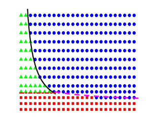
In figure 4, we explore the variations of the growth rate  $s$ for different
  ${\textit {El}}$. As
  ${\textit {El}}$ is increased from 0 to
  $0.01$, the growth rate of the disturbance shows a slight increase (figure 4b). As
  ${\textit {El}}$ is increased further, the growth rate shows a rapid decline. This indicates that the elasticity of the fluid plays a dual role in the analysis of jet stability: a viscoelastic jet composed of weakly elastic fluids exhibits more rapid growth of axisymmetric disturbances than a Newtonian one, while for viscoelastic jets with more pronounced elastic properties, the growth of axisymmetric disturbances is significantly suppressed. This feature is consistent with the experimental evidence for a laminar capillary jet of a viscoelastic fluid (Goldin et al. Reference Goldin, Yerushalmi, Pfeffer and Shinnar1969), and has not been reported in the existing theoretical analyses, to the best of our knowledge. We believe that the above behaviour is universal in the viscoelastic jet instability, and it is essentially related to the nonlinear constitutive relation of viscoelastic fluids and non-uniform basic velocity.

Figure 4. Variations of the growth rate  $s$ with the dimensionless axial wavenumber
  $k$ for different
  ${\textit {El}}$: (a)
  ${\textit {El}}=0.1, 0.3, 1, 5$; (b)
  ${\textit {El}}=0.001, 0.005, 0.01, 0.1$. Note that (b) shows the enlarged region near the maximum growth rate. Obviously, there are two peaks (denoted by
  $\mathrm {P}_{1}$ and
  $\mathrm {P}_{2}$) for
  ${\textit {El}}=1$ in (a), indicating that two different instability modes may appear at the corresponding locations (wavenumbers). With the help of the energy budget method, it can be further confirmed that
  $\mathrm {P}_{1}$ corresponds to elastic instability while
  $\mathrm {P}_{2}$ corresponds to shear instability (refer to the last paragraph in § 4.1 for detailed descriptions of the instabilities).
It is noticed that, for a uniform basic-velocity profiles, the elastic stress tensor  $\boldsymbol {\varGamma }=0 .$ Thus, all nonlinear terms in the rheological constitutive equations are eliminated after linearization, giving the same results as those obtained using the Jeffreys model. The instability analysis was thus regarded to be independent of the form of the constitutive equations (Goldin et al. Reference Goldin, Yerushalmi, Pfeffer and Shinnar1969; Ruo et al. Reference Ruo, Chen, Chung and Chang2011). However, when a non-uniform basic velocity is considered in the base-state solutions, as described in § 2.2, the nonlinear viscoelastic impacts will be preserved in the stability analysis. On the one hand, the non-uniform basic velocity induces a non-zero elastic stress tensor
  $\boldsymbol {\varGamma }$, including the unrelaxed axial elastic tension
  $\varGamma _{z z}$, based on the nonlinear constitutive equation. On the other hand, a coupling term between the elastic stress tensor and the perturbation velocity, i.e.
  $\langle \boldsymbol {\varGamma }, \tilde {\boldsymbol {V}}_{1}\rangle$ in (2.19), is derived from the linearization of the constitutive equation, which reflects the nonlinear characteristics of the constitutive equation to some extent. Strictly speaking, the term
  $\langle \tilde {\boldsymbol {T}}_{p}, \boldsymbol {U}_{1}\rangle$ in (2.19) is also from the linearization of the nonlinear part of the constitutive equation. However, its impact on the jet instability is small relative to the term
  $\langle \boldsymbol {\varGamma }, \tilde {\boldsymbol {V}}_{1}\rangle$ (see figure 8 for case B where the influence of
  $\langle \boldsymbol {\varGamma }, \tilde {\boldsymbol {V}}_{1}\rangle$ is removed and the DIP including the contribution of
  $\langle \tilde {\boldsymbol {T}}_{p}, \boldsymbol {U}_{1}\rangle$ is negligibly small). Therefore, the influence of nonlinear elasticity can be predicted through the coupling term
  $\langle \boldsymbol {\varGamma }, \tilde {\boldsymbol {V}}_{1}\rangle$.
Figure 5 shows the relative contribution of various factors in the rate of change of disturbance kinetic energy vs the wavenumber for different  ${\textit {El}}$. For small
  ${\textit {El}}$, the effects of surface tension (represented by SUT) and external gas shear and pressure (represented by SHG and PRG) are significant factors on the instability in the long-wave and short-wave regions, respectively (see figure 5a). With the increase of
  ${\textit {El}}$, the influence of fluid elasticity (represented by NE and DIP) begins to increase gradually and finally becomes dominant (figures 5(b) and 5(c)). It is notable that NE and DIP make completely opposite contributions to the rate of change of disturbance energy:
  $\mathrm {NE}$ tends to amplify the disturbance kinetic energy, thereby promoting the instability; on the contrary, DIP tends to reduce the kinetic energy of disturbance, thereby suppressing the jet instability. Note that
  $\mathrm {NE}$ is related to the unrelaxed elastic tension whereas DIP includes the influence of the coupling term
  $\langle \boldsymbol {\varGamma }, \tilde {\boldsymbol {V}}_{1}\rangle$ in the constitutive equation. The combined effect of
  $\mathrm {NE}$ and DIP is shown in figure 5(d). The NE is dominant for
  ${\textit {Wi}}< O(1)$, while DIP is dominant for
  ${\textit {Wi}}>O(1)$. In summary, the influence of fluid elasticity on the jet instability is mainly controlled by the magnitudes of NE and DIP, and the competition between NE and DIP is determined by
  ${\textit {Wi}}$.

Figure 5. Energy budget, using the relative rate of change of energy, vs the wavenumber for (a)  ${\textit {El}}=0.1$, (b)
  ${\textit {El}}=0.5$ and (c)
  ${\textit {El}}=1$. Here, the meanings of the letters can be found in table 4. Note that, in (c), the abrupt changes near
  $k \approx 1.2$ may be due to the increase in the calculation error caused by the mode transition (see figure 4(a) for
  ${\textit {El}}=1$). (d) Comparison of the relative sizes of
  $\mathrm {NE}$ and DIP with the change of
  ${\textit {Wi}}$. When
  ${\textit {Wi}}< O(1)$,
  $|\mathrm {NE}|>|\mathrm {DIP}|$, while for
  ${\textit {Wi}}>O(1)$,
  $|\mathrm {NE}|<|\mathrm {DIP}|$.
As is well known,  ${\textit {Wi}}$ quantifies the nonlinear response of the viscoelastic fluid (Galindo-Rosales et al. Reference Galindo-Rosales, Campo-Deaño, Sousa, Ribeiro and Pinho2014; Ding & Jian Reference Ding and Jian2021) (note that the factor
  ${\textit {Wi}}$ appears in front of the nonlinear terms of the constitutive equation (2.3)). Thus for
  ${\textit {Wi}}< O(1)$, the linear terms of the constitutive equation dominate the nonlinear parts, and the magnitude of NE exceeds the one of DIP (as shown in figure 5d), so that the perturbation growth rate shows an increasing trend. While for
  ${\textit {Wi}}>O(1)$, a strong nonlinear effect is stimulated, and the magnitude of DIP exceeds that of
  $\mathrm {NE}$, so that the perturbation growth rate shows a downward trend. This is consistent with the change of disturbance growth rate shown in figure 4(b), where the critical
  ${\textit {El}} \sim 0.01$ corresponds to
  ${\textit {Wi}} \sim 1$.
Figure 6 further shows the variations of the maximum perturbation growth rate with  ${\textit {Wi}}$. It is found that, when
  ${\textit {Wi}} < O(1)$, the viscoelastic jet is less stable than its Newtonian counterpart, since the nonlinear viscoelastic effect is insignificant and the unrelaxed tension promotes the instability of the jet. While in the range of
  ${\textit {Wi}} > O(1)$, the nonlinear viscoelastic effect greatly suppresses the maximum growth rate, which makes the viscoelastic jet more stable than the Newtonian one.

Figure 6. Variations of the maximum growth rate  $s_{\max }$
  $(s_{\max }=\max _{k}\{s\})$ with the Weissenberg number
  ${\textit {Wi}}$ for
  $(a)$
$(a)$  ${\textit {Re}}=100$ and
  $(b)$
$(b)$  ${\textit {Re}}=10$, where the green triangles (
 $\blacktriangle$, green) represent the shear instability (SI) modes and the blue circles (
 $\circ$, blue) represent the elastic instability (EI) modes (the detailed definitions of these instability modes are given in the penultimate paragraph in § 4.1). Here, the Newtonian maximum growth rate is also shown (dashed line) for reference. It is notable that the forms of the variations of the growth rate for different
  ${\textit {Re}}$ are unified by means of
  ${\textit {Wi}}$. Specifically, the growth rate of disturbance increases slightly with
  ${\textit {Wi}}< O(1)$, while it decreases rapidly with
  ${\textit {Wi}}>O(1)$.
In order to demonstrate the influences of the nonlinear elasticity and the unrelaxed elastic tension more clearly, we consider two specific cases: (i) using a linear viscoelastic model, i.e. the Jeffreys model  $-$ case
  $\mathrm {A}$, in which the unrelaxed axial elastic tension
  $\varGamma _{z z}$ and the coupling term
  $\langle \boldsymbol {\varGamma }, \tilde {\boldsymbol {V}}_{1}\rangle$ does not appear in spite of the non-uniform basic velocity considered; (ii) using the Oldroyd-B model with the coupling term
  $\langle \boldsymbol {\varGamma }, \tilde {\boldsymbol {V}}_{1}\rangle$ removed in (2.19) – case
  $\mathrm {B}$. In case
  $\mathrm {A}$, the influences of both the unrelaxed elastic tension and nonlinear elasticity are eliminated at the same time. Compared with the full Oldroyd-B model, case
  $\mathrm {B}$ is able to show the effect of
  $\varGamma _{z z}$ alone without being limited by the nonlinear factors.
The variations of the growth rate  $s$ of disturbance for cases
  $\mathrm {A}$ and
  $\mathrm {B}$ are shown in figures 7(a) and 7(b), respectively. As
  ${\textit {El}}$ is increased from 0 to
  $0.1$ in case
  $A$, the growth rate shows a slight increase, and when
  ${\textit {El}}$ continues to increase, the growth rate reaches saturation and hardly changes. The slight promotion effect of linear viscoelasticity on the growth rate is consistent with the above analysis. However, for case
  $\mathrm {B}$, the growth rate increases continuously with
  ${\textit {El}}$ due to the presence of the unrelaxed elastic tension. In other words, the unrelaxed elastic tension further promotes the increase in the growth rate of the disturbance. Compared with the full Oldroyd-B model, the downward trend of the growth rate does not appear due to the lack of the nonlinear elasticity. From the perspective of energy budget analysis, as shown in figure 8,
  $\mathrm {NE}$ becomes dominant in the jet instability and promotes the increase in the growth rate with the increase of
  ${\textit {El}}$ for case B. It is notable that the contribution of the DIP term related to the nonlinear elasticity effect on the growth rate of the disturbance is almost negligible in case B. Comparing with the full Oldroyd-B model, this illustrates the significance of the coupling term
  $\langle \boldsymbol {\varGamma }, \tilde {\boldsymbol {V}}_{1}\rangle$ in the nonlinear elastic behaviour of the jet.

Figure 7. Variations of the growth rate  $s$ of (a) the Jeffreys model – case A and (b) the Oldroyd-B model without the coupling term
  $\langle \boldsymbol {\varGamma }, \tilde {\boldsymbol {V}}_{1}\rangle$ – case
  $\mathrm {B}$, vs the wavenumber
  $k$ for different
  ${\textit {El}}$. Note that
  $(a)$ shows the enlarged region near the maximum growth rate, like figure 4(b). It can be observed that, when
  ${\textit {El}}>0.1$, the growth rate in case A hardly changes with the increase of
  ${\textit {El}}$, whereas the growth rate in case B continues to increase with
  ${\textit {El}}$.

Figure 8. Energy budget, using the relative rate of change of energy, vs the wavenumber for case B, where (a)  ${\textit {El}} = 0.1$ and (b)
  ${\textit {El}} = 0.5$.
In the linear and nonlinear regimes of fluid elasticity, the structure of the spectrum is also different, which is discussed in detail in Appendix B. In the linear regime (i.e.  ${\textit {Wi}}< O(1))$, the ring structure in the viscoelastic spectrum is prominent, whereas in the nonlinear regime
  $({\textit {Wi}}>O(1))$, the ring collapses into the continuous spectra in an irregular manner. In addition, by tracking its trajectory, we find the most unstable eigenvalue falls into the continuous spectrum balloon when
  $(1-X) {\textit {El}} \sim 1$, which leads to a sharp deterioration in the accuracy and convergence for resolving the most unstable eigenvalue.
Based on the energy analysis, three different types of instability mechanism can be identified in the present work. First, similar to the case of Newtonian jets, the predominance of the SUT term characterizes the instability caused by surface tension, which can be called the capillary instability (abbreviated as  $\mathrm {CI}$), while the predominance of SHG or PRG corresponds to the instability caused by external gas shear and pressure, called the shear instability (abbreviated as SI). In addition, a new instability mechanism can be identified, where the elastic effect (i.e. NE) plays a dominant role in the instability of a viscoelastic jet, and this instability is called the elastic instability (abbreviated as EI). The previous analysis of figures 4–8 is helpful to understand the mechanism and features of EI. Importantly, the nonlinear elastic effect in the EI regime plays a stabilizing role in the jet.
With the help of energy budget analysis and identification of instability modes, we can explore the instability mechanisms in figure 4(a), and determine the instability modes at the peaks (denoted by  $\mathrm {P}_{1}$ and
  $\mathrm {P}_{2}$). For small
  ${\textit {El}}$ (e.g.
  ${\textit {El}}=0.1$), the instability of a jet is attributed to SI since the contributions of SHG and PRG to the instability are dominant at the most dangerous disturbance wavenumber
  $k \approx 1$ (figure 5a). As
  ${\textit {El}}$ increases to 1, the elastic effect becomes enhanced, and the instability of the jet belongs to EI in the long-wave region, while SI is still the main instability mode in the short-wave region (figure 5c). Comparing the maximum growth rates in the long-wave and short-wave regions, it can be seen that the maximum growth rate in the long-wave region is significantly larger (figure 4a), and thus the dominant mechanism of instability for
  ${\textit {El}} = 1$ in figure 4(a) is attributed to EI. In this paper, we mainly focus on the instability corresponding to the maximum growth rate over the entire wavelength range.
4.2. General features of instability modes
To gain more insight into the instability, we depict the variations in the maximum growth rate over the entire wavelength range, i.e.  $s_{\max }=\max _{k}\{s\}$, and the corresponding phase speed,
  $c_{r,\max }$, with the relevant parameters in figure 9. Note that the unstable eigenvalues are usually located on the
  $I_{1}$ branch (figure 13), but this does not mean that the external gas does not contribute to the instability. In fact, we have known from the analysis in § 4.1 that the effect of external gas is the source of SI. As
  ${\textit {El}}$ increases, the transition of the instability mode from CI (or SI) to EI occurs (see figure 9a), as expected. In the EI regime, the growth rate decreases approximately linearly with
  ${\textit {El}}$. In addition, the transitions from SI (or EI) to CI and from CI to SI occur with the increase of
  ${\textit {We}}^{-1}$ and
  $K$, respectively (figures 9(c) and 9(e)). The growth rates in the CI and SI regimes increase approximately linearly with
  ${\textit {We}}^{-1}$ and
  $K$, respectively. The phase diagrams on the mode transitions in different parameter spaces will be given in § 4.3.

Figure 9. Variations of the maximum growth rate  $s_{\max }$ and the corresponding phase speed
  $c_{r,\max }$ of disturbances with (a,b)
  ${\textit {El}}$, (c,d)
  ${\textit {We}}^{-1}$ and (e,f)
  $K$ for a fixed
  ${\textit {El}}=0.01$. Here,
  ${\textit {Re}}=100$,
  $Q=0.0013$,
  $N=0.018$,
  $U_{s}=1.2$. The red squares represent the CI modes, the green triangles represent the SI modes and the blue circles represent the EI modes. In (b,d), the dimensionless average velocity
  $U_{m}$ of the jet at the basic state is shown for reference. The growth rate in the EI regime in (a) decreases approximately linearly with the increase of
  ${\textit {El}}$, while the growth rates increase approximately linearly with the increase of
  ${\textit {We}}^{-1}$ and
  $K$ in the
  $\mathrm {CI}$ and SI regimes of (c,e), respectively.
With increasing  ${\textit {El}}$, the phase speed
  $c_{r}$ in the EI regime decreases and tends to the basic velocity at the centre of the internal fluid (i.e.
  $c_{r} \rightarrow 1$ in figure 9b), so the EI mode can be also called the centre mode. This feature is analogous to the centre mode instability in viscoelastic Poiseuille flow (Garg et al. Reference Garg, Chaudhary, Khalid, Shankar and Subramanian2018; Khalid et al. Reference Khalid, Chaudhary, Garg, Shankar and Subramanian2021). In figure 9(d), with the decrease of
  ${\textit {We}}$, the phase speed in the CI regime decreases (suppressed), and then gradually tends to a constant value. However, the phase speed in the CI regime is always above the average velocity of the jet, and stays near the velocity
  $U_{s}$ at the jet interface, so the CI mode can be also called the interface mode. In figure 9(f), it can be observed that, as
  $K$ increases, the phase speed in the SI regime increases (promoted), which tends to the velocity in the shear layer of the external gas, so the SI mode can be called the shear mode. The above features on the growth rate and phase speed under the three instability modes are summarized in table 5.
Table 5. The features on the growth rate and phase speed for the instability modes CI, SI and EI.

The velocity and polymer stress eigenfunctions corresponding to the unstable eigenvalues are shown in figure 10. It can be found that, as  ${\textit {El}}$ increases, the axial velocity eigenfunctions gradually approach the centre of the jet (i.e.
  $r=0$) in the EI regime, which is consistent with the behaviour of the eigenvalues, although the eigenfunctions are not localized near the centreline. In contrast, the axial disturbance velocity fields are almost uniform, spreading across the cross-section of the liquid jet for the parameters considered in the CI regime (corresponding to small
  ${\textit {We}}$; see figure 10c). The amplitude of the axial velocity eigenfunction in figure 10(d) is significantly larger near the interface (i.e.
  $r \approx 1$) than that at the centre due to the dominance of the shearing effect in the SI regime. In addition, the
  $\hat {\tau }_{z z}$ eigenfunction shows a sharp peak for large
  ${\textit {El}}$ near the boundary layer of the liquid jet, in which a large velocity gradient appears for the basic velocity.

Figure 10. Profiles of the axial (a) velocity and (b) polymer stress of the disturbance corresponding to unstable eigenvalues at different  ${\textit {El}}$ with
  $k=0.8$,
  $X=0.9$,
  ${\textit {Re}}=100$,
  ${\textit {We}}=3$,
  $U_{s}=1.2$ and
  $K=0.9$. (c,d) Show the profiles of the axial velocity of the disturbance at different
  ${\textit {We}}$ and
  $K$, respectively, with
  ${\textit {El}}=0.1$. Here, the moduli of the velocity and stress are calculated because they are complex variables. In (a) the axial velocity profiles for large
  ${\textit {El}}$ correspond to EI modes, while in (c) the velocity profiles for small
  ${\textit {We}}$ correspond to CI modes and in (d) the velocity profiles correspond to SI modes.
4.3. Transitions of instability modes in parameter space
In the previous section, we have analysed the characteristics of the three instability modes in detail. In this section, we focus on the transition boundaries between different modes (i.e. CI/SI, CI/EI and SI/EI) in parameter space.
Figure 11(a) shows the transition between  $\mathrm {CI}$ and SI on a
  ${\textit {We}}$–
 $K$ plane for very small
  ${\textit {El}}$
  $({\textit {El}}= 0.01)$. As
  ${\textit {We}}$ or
  $K$ increases, the transition of the instability mode from CI to EI occurs. The transition boundary of CI/SI is found to approximately satisfy the curve
  $l_1$:
  $K {\textit {We}}=c_{1}$, with the constant
  $c_{1}$ depending on
  ${\textit {Re}}$ (see table 7). As
  ${\textit {El}}$ increases, the EI mode appears, which has been known from the previous discussion. Figure 11(b) shows the transition between CI and EI on a
  ${\textit {El}}$–
 $K$ plane for small
  ${\textit {We}}$
  $({\textit {We}}=0.5)$. Note that a large value of
  $K$ means a large velocity gradient for the basic velocity of the jet (see (2.12)), thereby resulting in a large unrelaxed axial elastic tension
  $\varGamma _{z z}$, which makes the EI tend to dominate even at a small value of
  ${\textit {El}}$. The transition boundary of
  $\mathrm {CI} / \mathrm {EI}$ is found to approximately satisfy the curve
  $l_{2}$:
  ${\textit {We}}^{\gamma }(1-X) {\textit {El}}\,K^{\alpha }=c_{2}$ with
  $\alpha =3$ and
  $\gamma =1.5$, where the constant
  $c_{2}$ depends on
  ${\textit {Re}}$.

Figure 11. (a) Phase diagram of CI/SI mode on a  ${\textit {We}}$–
 $K$ plane at
  ${\textit {Re}} = 200$,
  ${\textit {El}} = 0.01$ and
  $X = 0.9$. (b) Phase diagram of CI/EI mode on a
  ${\textit {El}}$–
 $K$ plane at
  ${\textit {We}} = 0.5$,
  ${\textit {Re}} = 50$ and
  $X = 0.8$. (c) Phase diagrams of CI/SI, CI/EI and SI/EI on a
  ${\textit {El}}$–
 $K$ plane at
  ${\textit {We}} = 3$,
  ${\textit {Re}} = 50$,
  $X = 0.8$. (d) Phase diagrams of CI/SI, CI/EI and SI/EI on a
  ${\textit {El}}$–
 ${\textit {We}}$ plane at
  ${\textit {Re}} = 100$,
  $K = 0.9$ and
  $X = 0.8$. The red squares (
 $\blacksquare$, red) represent the CI mode, the green triangles (
 $\blacktriangle$, green) represent the SI mode and the blue circles (
 $\circ$, blue) represent the EI mode. The transition boundary of CI/SI mode is close to the curve
  $l_1$:
  $K{\textit {We}}=c_1$; the transition boundary of CI/EI mode is close to the curve
  $l_{2}$:
  ${\textit {We}}^{\gamma }(1-X) {\textit {El}}\,K^{\alpha }=c_{2}$ with
  $\alpha =3$ and
  $\gamma =1.5$; while the transition boundary of SI/EI mode is close to the curve
  $l_{3}$:
  $(1-X) {\textit {El}}\,K^{\beta }=c_{3}$ with
  $\beta =1$. Here, the constants
  $c_1$,
  $c_2$ and
  $c_3$ depend on
  ${\textit {Re}}$, which are listed in table 7. Note that, in (c), the boundary curve
  $l_1$ of CI/SI is a horizontal line on a
  ${\textit {El}}$–
 $K$ plane for a fixed
  ${\textit {We}}$. In (d) the boundary curves
  $l_1$ and
  $l_3$ of CI/SI and SI/EI are the horizontal and vertical lines, respectively, on a
  ${\textit {El}}$–
 ${\textit {We}}$ plane for fixed
  $K$ and
  $X$.
$X$.
For certain parameter ranges (e.g. small  ${\textit {El}}$ or
  ${\textit {We}}$), only two instability modes and their transitions (e.g. CI/SI or CI/EI) can be observed (figures 11(a) and 11(b)). While, for large
  ${\textit {El}}$ or
  ${\textit {We}}$, three instability modes and their transitions are usually observed. Figures 11(c) and 11(d) show the transition boundaries of CI/SI, CI/EI and SI/EI on a
  ${\textit {El}}$–
 $K$ or
  ${\textit {El}}$–
 ${\textit {We}}$ plane, where the curves
  $l_1$ and
  $l_2$ are still valid at large
  ${\textit {We}}$ (e.g.
  ${\textit {We}} = 3$) for the transition boundaries of CI/SI and CI/EI, respectively. Furthermore, the transition boundary of SI/EI is approximately given by the curve
  $l_3$:
  $(1-X){\textit {El}}\,K^{\beta }=c_3$ with
  $\beta =1$. In all cases, the transition boundaries of CI/SI, CI/EI and SI/EI and the values of
  $c_1$,
  $c_2$ and
  $c_3$ are summarized in tables 6 and 7, respectively. Note that the transition boundary of CI/SI is a straight line on the
  ${\textit {El}}-K$ plane with a fixed
  ${\textit {We}}$ or on the
  ${\textit {El}}$–
 ${\textit {We}}$ plane with a fixed
  $K$, and the transition boundary of SI/EI is a straight line on the
  ${\textit {El}}$–
 ${\textit {We}}$ plane for a fixed
  $K$ (figures 11(c) and 11(d)).
Table 6. The approximate transition boundaries between different modes (CI/SI, CI/EI and SI/EI) in the parameter space, where the constants  $c_{1}, c_{2}$ and
  $c_{3}$ depend on
  ${\textit {Re}}$ and their values are provided in table 7.

Table 7. The values of  $c_{1}, c_{2}$ and
  $c_{3}$ are provided for different
  ${\textit {Re}}$.

Figure 12 displays the variations of the transition boundaries of CI/SI, CI/EI and SI/EI with related parameters. From figure 12(a), it can be found that the boundary of CI/SI would shift up as  ${\textit {Re}}$ increases, i.e. the CI region expands and the SI region shrinks, because the constant
  $c_1$ increases with the increase of
  ${\textit {Re}}$. The boundary of CI/EI varies slightly with
  ${\textit {Re}}$ due to the weak dependence of
  $c_2$ on
  ${\textit {Re}}$ (figure 12b). In figure 12(c), the boundary of CI/EI would shift down as
  ${\textit {We}}$ increases, i.e. the CI region would shrink, which is consistent with the fact that a large
  ${\textit {We}}$ characterizes relatively small surface tension. While for large
  $X$, i.e. a large solvent component, the influence of fluid elasticity is weakened, resulting in the contraction of the EI region (figures 12(d) and 12(f)). In addition, since the constant
  $c_3$ decreases with the increase of
  ${\textit {Re}}$ (see table 7), the boundary of SI/EI would shift down as
  ${\textit {Re}}$ increases (figure 12e).

Figure 12. Variations of the transition boundaries of CI/SI, CI/EI and SI/EI with related parameters, where (a)  ${\textit {El}} = 0.01$ and
  $X = 0.9$ with
  ${\textit {Re}} = 50$, 100, 400; (b)
  ${\textit {We}} = 0.5$ and
  $X = 0.8$ with
  ${\textit {Re}} = 50$, 100, 400; (c)
  ${\textit {Re}} = 100$ and
  $X = 0.8$ with
  ${\textit {We}} = 0.5$, 1, 3; (d)
  ${\textit {Re}} = 100$ and
  ${\textit {We}} = 0.5$ with
  $X = 0.7$, 0.8, 0.9; (e)
  ${\textit {We}} = 3$ and
  $X = 0.8$ with
  ${\textit {Re}} = 50$, 100, 400; (f)
  ${\textit {Re}} = 100$ and
  ${\textit {We}} = 3$ with
  $X = 0.7$, 0.8, 0.9.
5. Conclusions
The present study provides a comprehensive account of the linear instability of viscoelastic jets, where the importance of a non-uniform basic velocity is clarified for the first time. Especially, a new unrelaxed axial elastic tension is derived based on a non-uniform basic velocity, which is significantly different from Goren & Gottlieb's theory. The unrelaxed elastic tension depends on the velocity gradient, elasticity number and solvent viscosity ratio. To carry out the linear stability analysis, the base state is subjected to small amplitude axisymmetric disturbances. After neglecting high-order terms, the linearized governing equations together with the linearized boundary conditions can be derived, which constitute a generalized eigenvalue problem. Despite its complexity, we successfully solve this problem by employing a spectral collocation method. Furthermore, to better understand the mechanism of jet instability, an analysis of the energy budget of the destabilization process is performed over a control volume of one disturbance wavelength.
Our results show that the elasticity of fluid plays a dual role in the analysis of jet stability: a viscoelastic jet composed of weakly elastic fluids exhibits more rapid growth of axisymmetric disturbances than a Newtonian one, while for viscoelastic jets with more pronounced elastic properties, the growth of axisymmetric disturbances is significantly suppressed. This feature is essentially related to the nonlinear constitutive relation of viscoelastic fluids and the non-uniform basic velocity. When  ${\textit {Wi}}< O(1)$, the linear terms of the constitutive equation dominate the nonlinear parts, and the linear elasticity of fluids leads to an increase in the growth rate of disturbance. While when
  ${\textit {Wi}}>O(1)$, a strong nonlinear effect is stimulated by the coupling term
  $\langle \boldsymbol {\varGamma }, \tilde {\boldsymbol {V}}_{1}\rangle$ between the elastic stress tensor and perturbation velocity, where the non-zero elastic stress tensor is induced by non-uniform basic velocity. The nonlinear elasticity of fluids has a significant inhibitory effect on the disturbance growth rate. These assertions are supported by the results of the energy analysis, and are further verified by considering two specific cases: (i) using a linear viscoelastic model, i.e. the Jeffreys model – case A; (ii) using the nonlinear Oldroyd-B model with the coupling term
  $\langle \boldsymbol {\varGamma }, \tilde {\boldsymbol {V}}_{1}\rangle$ removed – case
  $\mathrm {B}$
Based on the energy budget analysis, three different instability mechanisms can be identified, which correspond to three instability modes, i.e. the capillary instability (CI), shear instability (SI) and elastic instability (EI) modes. For the CI mode, the surface tension is dominant in the jet instability; for the SI mode, the shear and pressure of external gas are dominant in the jet instability; and for the EI mode, the elastic tension plays a dominant role in the jet instability. The general features of these instability modes are explored. It is found that both the growth rate and phase speed of the disturbances are promoted in the SI regime, while they are both suppressed in the EI regime. In contrast, the growth rate in the CI regime is promoted, whereas the phase speed in the CI regime is suppressed. Furthermore, in the EI regime, the phase speed tends to the basic velocity at the centre of the jet and the corresponding velocity eigenfunction also gradually approaches the centre as  ${\textit {El}}$ increases, but the eigenfunction is not localized near the centreline. Although the phase speed in the CI regime is also decreasing, it is always above the average velocity of the jet, which means that it does not tend to the basic velocity at the centre, and the corresponding velocity eigenfunction is almost uniform, spreading across the cross-section of the liquid jet. In contrast, the phase speed in the SI regime is increasing, and tends to the velocity in the shear layer of the external gas, and the amplitude of the corresponding velocity eigenfunction is significantly larger near the interface due to the dominance of the shearing effect in the SI regime. In addition, the eigenfunction for the axial elastic stress shows a sharp peak near the boundary layer of the liquid jet, where a large velocity gradient appears in the basic velocity.
Finally, we investigate the transitions of instability modes in parameter spaces and provide the transition boundaries between different modes (i.e. CI/SI, CI/EI and SI/EI). This study provides guidance for understanding the mechanism of instability of viscoelastic jets in a co-flowing gas stream and the transition criterion of instability modes.
Funding
This work was supported by the National Natural Science Foundation of China (Z.D., grant number 11902165), (T.S., grant numbers 12027801, 11621202), (K.M., grant number 11902318), (Y.J., grant number 11772162); the Youth Innovation Promotion Association CAS (T.S., grant number 2018491); and the Natural Science Foundation of Inner Mongolia Autonomous Region of China (Z.D., grant number 2019BS01004).
Declaration of interests
The authors report no conflict of interest.
Appendix A. The linearized governing equations and boundary conditions
Substituting (2.22) into the governing equations (2.16)–(2.21), we obtain the following set of linearized governing equations:
 $$\begin{gather} \hat{v}_{1}^{\prime}+\frac{1}{r} \hat{v}_{1}+\mathrm{i} k \hat{u}_{1}=0, \end{gather}$$
 $$\begin{gather}\mathrm{i} k\left(U_{1}-c\right) \hat{v}_{1}={-}\hat{p}_{1}^{\prime}+\frac{X}{{\textit{Re}}}\left[\hat{v}_{1}^{\prime \prime}+\frac{1}{r} \hat{v}_{1}^{\prime}-\frac{1}{r^{2}} \hat{v}_{1}-k^{2} \hat{v}_{1}\right]+\hat{\tau}_{r r}^{\prime}+\frac{1}{r} \hat{\tau}_{rr}+\mathrm{i} k \hat{\tau}_{rz}-\frac{1}{r} \hat{\tau}_{\theta\theta}, \end{gather}$$
 $$\begin{gather}\mathrm{i} k\left(U_{1}-c\right) \hat{u}_{1}={-}U_{1}^{\prime} \hat{v}_{1}-\mathrm{i} k \hat{p}_{1}+\frac{X}{{\textit{Re}}}\left[\hat{u}_{1}^{\prime \prime}+\frac{1}{r} \hat{u}_{1}^{\prime}-k^{2} \hat{u}_{1}\right]+\hat{\tau}_{r z}^{\prime}+\frac{1}{r} \hat{\tau}_{r z}+\mathrm{i} k \hat{\tau}_{z z}, \end{gather}$$
 $$\begin{gather}\left[1+\mathrm{i} k {\textit{Wi}}\left(U_{1}-c\right)\right] \hat{\tau}_{r r}=2 \mathrm{i} k(1-X) {\textit{El}} U_{1}^{\prime} \hat{v}_{1}+2 \frac{1-X}{{\textit{Re}}} \hat{v}_{1}^{\prime}, \end{gather}$$
 \begin{gather} {\left[1+\mathrm{i} k {\textit{Wi}}\left(U_{1}-c\right)\right] \hat{\tau}_{r z}+{\textit{Wi}}\left[{-}U_{1}^{\prime} \hat{\tau}_{rr}+\frac{1-X}{{\textit{Re}}} U_{1}^{\prime \prime} \hat{v}_{1}-2 \mathrm{i} k(1-X) {\textit{El}}\left(U_{1}^{\prime}\right)^{2} \hat{v}_{1}\right.} \nonumber\\ \quad \left.-\frac{1-X}{{\textit{Re}}}U_{1}^{\prime}\left(\hat{v}_{1}^{\prime}+\mathrm{i} k \hat{u}_{1}\right)\right]=\frac{1-X}{{\textit{Re}}}\left(\hat{u}_{1}^{\prime}+\mathrm{i}k \hat{v}_{1}\right),\end{gather}
 \begin{gather} \left[1+\mathrm{i} k {\textit{Wi}}\left(U_{1}-c\right)\right] \hat{\tau}_{\theta \theta}= \frac{2(1-X)}{{\textit{Re}}} \frac{\hat{v}_{1}}{r}, \end{gather}
 \begin{gather} \left[1+\mathrm{i} k {\textit{Wi}}\left(U_{1}-c\right)\right] \hat{\tau}_{zz}-2 {\textit{Wi}}\, U_{1}^{\prime} \left[\hat{\tau}_{r z}-2(1-X) {\textit{El}}\,U_{1}^{\prime \prime} \hat{v}_{1}+2 \mathrm{i} k(1-X) {\textit{El}}\, U_{1}^{\prime} \hat{u}_{1} \vphantom{\frac{1-X}{{\textit{Re}}}}\right. \nonumber\\ \quad \left.+\frac{1-X}{{\textit{Re}}} \hat{u}_{1}^{\prime}\right]= \frac{2(1-X)}{{\textit{Re}}} \mathrm{i} k \hat{u}_{1}, \end{gather}
 $$\begin{gather} \hat{v}_{2}^{\prime}+\frac{1}{r} \hat{v}_{2}+\mathrm{i} k \hat{u}_{2}=0, \end{gather}$$
 $$\begin{gather}\mathrm{i} k\left(U_{2}-c\right) \hat{v}_{2}={-}\frac{1}{Q} \hat{p}_{2}^{\prime}+\frac{1}{{\textit{Re}}} \frac{N}{Q}\left[\hat{v}_{2}^{\prime \prime}+\frac{1}{r} \hat{v}_{2}^{\prime}-\frac{1}{r^{2}} \hat{v}_{2}-k^{2} \hat{v}_{2}\right], \end{gather}$$
 $$\begin{gather}\mathrm{i} k\left(U_{2}-c\right) \hat{u}_{2}={-}U_{2}^{\prime} \hat{v}_{2}-\frac{\mathrm{i} k}{Q} \hat{p}_{2}+\frac{1}{{\textit{Re}}} \frac{N}{Q}\left[\hat{u}_{2}^{\prime \prime}+\frac{1}{r} \hat{u}_{2}^{\prime}-k^{2} \hat{u}_{2}\right]. \end{gather}$$
Here, the prime denotes the derivative with respect to  $r$.
$r$.
For the boundary conditions, the velocity and pressure at the symmetry axis satisfy the consistency conditions
 \begin{equation} \hat{v}_{1}=\hat{u}_{1}^{\prime}=\hat{p}_{1}^{\prime}=0, \quad \text{at } r=0. \end{equation}
At the liquid–gas interface, the continuity of velocity, the kinematic boundary condition and the balance of the normal and tangential stresses are satisfied, i.e.
 $$\begin{gather} \hat{v}_{1}=\hat{v}_{2}, \end{gather}$$
 $$\begin{gather}\hat{u}_{1}-\hat{u}_{2}+\left(U_{1}^{\prime}-U_{2}^{\prime}\right) \hat{\eta}=0, \end{gather}$$
 $$\begin{gather}{\rm i} k\left(U_{1}-c\right) \hat{\eta}=\hat{v}_{1}, \end{gather}$$
 $$\begin{gather}\hat{p}_{1}-\hat{p}_{2}+\frac{2 N}{{\textit{Re}}} \hat{v}_{2}^{\prime}-\frac{2 X}{{\textit{Re}}} \hat{v}_{1}^{\prime}-\hat{\tau}_{r r}={-}\frac{1}{{\textit{We}}}\left(1-k^{2}\right) \hat{\eta}, \end{gather}$$
 $$\begin{gather}\frac{N}{{\textit{Re}}} U_{2}^{\prime \prime} \hat{\eta}+\frac{N}{{\textit{Re}}}\left(\hat{u}_{2}^{\prime}+\mathrm{i} k \hat{v}_{2}\right)=\frac{1}{{\textit{Re}}} U_{1}^{\prime \prime} \hat{\eta}+\frac{X}{{\textit{Re}}}\left(\hat{u}_{1}^{\prime}+\mathrm{i} k \hat{v}_{1}\right)-2 \mathrm{i} k(1-X) {\textit{El}}\left(U_{1}^{\prime}\right)^{2} \hat{\eta}+\hat{\tau}_{rz}, \end{gather}$$
at  $r=1$.
At the outside boundary,
 \begin{equation} \hat{v}_{2}=\hat{u}_{2}^{\prime}=\hat{p}_{2}^{\prime}=0, \quad \text{at } r=a, \end{equation}
with  $a=R_{2} / R_{1}$.
Appendix B. Eigenspectrum of viscoelastic jets
Using the numerical method in § 2.4, the viscoelastic jet spectrum can be obtained. Figure 13 shows the eigenspectrum for an Oldroyd-B jet, where the spectrum for a Newtonian jet with the same configuration is also shown for reference. It can be found that the structure of spectrum is composed of two separate parts (denoted by  $I_{1}$ and
  $I_{2}$), for both Newtonian and viscoelastic jets. On the
  $I_{1}$ branch, the real parts of the eigenvalues on the centreline approach the dimensionless velocity of the internal fluid (i.e. the phase speed
  $c_{r} \approx 1$), which means that the
  $I_{1}$ branch is related to the internal fluid. While for the
  $I_{2}$ branch, the real parts of most eigenvalues are concentrated near the dimensionless velocity of the external gas (i.e.
  $c_{r} \approx Q^{-1 / 2} \approx 27$), so the
  $I_{2}$ branch is related to the external gas. For the
  $I_{2}$ branch, a characteristic ‘Y-shaped’ structure can be observed, which is well known for Poiseuille flow of a Newtonian fluid (Schmid & Henningson Reference Schmid and Henningson2001). In contrast to the case of Newtonian jets, a ring structure appears on the
  $I_{1}$ branch for the low
  ${\textit {El}}$ in viscoelastic spectra. Similar to the cases of viscoelastic plane and pipe flows, the ring structure originates from the discrete high-frequency Gorodtsov–Leonov modes (refer to Chaudhary et al. Reference Chaudhary, Garg, Subramanian and Shankar2021). This demonstrates the viscoelastic jet spectrum differs substantially from its Newtonian counterpart. As
  ${\textit {El}}$ is increased from
  $10^{-4}$ to
  $10^{-3}$ (
 ${\textit {Wi}}$ from 0.01 to 0.1), the ring structure gets smaller in size (see figure 16). Interestingly, for Jeffreys viscoelastic jets, the ring falls off from the
  $I_{1}$ branch with the increase of
  ${\textit {El}}$, in contrast with the case of Oldroyd-B viscoelastic jets (figure 16).

Figure 13. Eigenspectra of the jet for (a) Oldroyd-B ( ${\textit {El}}=2 \times 10^{-4}$ and
  $X=0.9$) and (c) Newtonian fluids, at
  $k=1$,
  ${\textit {Re}}=100$,
  ${\textit {We}}=3$,
  $Q=0.0013$,
  $N=0.018$,
  $U_{s}=1.2$,
  $K=0.9$; (b,d) show the enlarged regions near the unstable eigenvalue (marked by the red circle) in (a,c), respectively. In order to ensure the accuracy, the eigenspectra are obtained using
  $N_{1}=120$ and
  $N_{2}=100$. For both Newtonian and viscoelastic jets, the structure of spectrum is composed of two separate parts (denoted by
  $I_{1}$ and
  $I_{2}$): the
  $I_{1}$ branch corresponds to the internal fluid (liquid); while the
  $I_{2}$ branch corresponds to the external gas. Obviously, the unstable eigenvalues are usually located on the
  $I_{1}$ branch. In contrast to the Newtonian case, a ring structure appears on the
  $I_{1}$ branch in viscoelastic spectra. However, for small
  ${\textit {El}}$, the eigenspectra of the Oldroyd-B and Newtonian jets near the unstable eigenvalue are similar (see (b,d)).
With increasing  ${\textit {El}}$ (ranging from
  $10^{-3}$ to
  $0.05$) or equivalently
  ${\textit {Wi}}$ (ranging from
  $0.1$ to 5) for a fixed
  ${\textit {Re}}$, figure 14 shows the ring structure of the viscoelastic spectrum is altered in a singular manner. Meanwhile, a visible feature is the appearance of two continuous spectra (CS) located in the centre of the ring structure. It is now well understood that the
  $\mathrm {CS}$ arise from the local nature of the constitutive model for the polymeric stress (Graham Reference Graham1998; Chaudhary et al. Reference Chaudhary, Garg, Subramanian and Shankar2021; Roy et al. Reference Roy, Garg, Reddy and Subramanian2021). Specifically, the origin of the CS in viscoelastic flows can be traced to the singularity which arises when the coefficient of the highest-order derivative in the differential equation governing the stability vanishes. Similar to the cases of viscoelastic plane and pipe flows (Chaudhary et al. Reference Chaudhary, Garg, Subramanian and Shankar2021; Khalid et al. Reference Khalid, Chaudhary, Garg, Shankar and Subramanian2021), this coefficient turns out to be the product
  $[1+\mathrm {i} k {\textit {Wi}}(U_{1}-c)][1+\mathrm {i} k X {\textit {Wi}}(U_{1}-c)]$. This leads to a pair of horizontal ‘lines’ in the
  $c_{r}-c_{i}$ plane with
  $c_{i}=-1 / k {\textit {Wi}}$ and
  $c_{i}=-1 / k X {\textit {Wi}}$, respectively, and with
  $\min \{U_{1}\} \leq c_{r} \leq \max \{U_{1}\}$ for the two
  $\mathrm {CS}$. Henceforth, these two continuous spectra are respectively abbreviated as ‘CS1’ and ‘CS2’, where CS1 with
  $c_{i}=-1 / k {\textit {Wi}}$ is present even in the absence of solvent (i.e.
  $X=0)$ and CS2 with
  $c_{i}=-1 / k X {\textit {Wi}}$ is present only for a non-zero
  $X$.
$X$.

Figure 14. Eigenspectra of the jet for an Oldroyd-B fluid at  $k=1$,
  ${\textit {Re}}=100$,
  ${\textit {We}}=3$,
  $X=0.9$,
  $Q=0.0013$,
  $N=0.018$,
  $U_{s}=1.2$ and
  $K=0.9$, with
  ${\textit {El}}$ ranging from
  $1 \times 10^{-3}$ to
  $0.05$ (equivalently,
  ${\textit {Wi}}$ ranging from 0.1 to 5): (a)
  ${\textit {El}} =1 \times 10^{-3}$
  $({\textit {Wi}}=0.1)$; (b)
  ${\textit {El}}=5 \times 10^{-3}$
  $({\textit {Wi}}=0.5)$; (c)
  ${\textit {El}}=0.01$
  $({\textit {Wi}}=1)$ and (d)
  ${\textit {El}}=0.05$
  $({\textit {Wi}}=5)$. The eigenspectra are obtained using
  $N_{1}=200$ and
  $N_{2}=120$. Here, we concentrate on showing the change of the ring structure on the
  $I_{1}$ branch, since there is no obvious change of the ‘Y-shaped’ structure of the
  $I_{2}$ branch. The ring structure is prominent at the lower
  ${\textit {El}}$, but is absent beyond
  ${\textit {El}} \sim 10^{-2}$ or
  ${\textit {Wi}} \sim$ 1. The locations of the CS1 and CS2 lines are shown for reference, where
  $c_{i}=-1 / k {\textit {Wi}}$ and
  $-1 / k X {\textit {Wi}}$, respectively, and
  $c_{r} \in [\min \{U_{1}\}, \max \{U_{1}\}]=[1,1.2]$ (note that
  $U_{s}=1.2$) for the two
  $\mathrm {CS}$. The eigenvalue with
  $c_{i}>0$ is the unstable one.
The ring surrounds the continuous spectra at small  ${\textit {El}}$ of
  $O(\sim 10^{-3})$. As
  ${\textit {Wi}}$ or
  ${\textit {El}}$ is increased, both CS1 and CS2 get closer to zero, and at the same time, the ring moves towards the CS with the ring getting smaller in size (figures 14(a) and 14(b)). Note that the size of the CS (i.e. the range of
  $c_r$) is constant. For
  ${\textit {El}} \sim 10^{-2}$ (i.e.
  ${\textit {Wi}} \sim 1$), the ring structure is distorted and for higher
  ${\textit {El}}$
  $({\textit {Wi}})$ the modes originally on the ring collapse into the
  $\mathrm {CS}$ in an irregular manner (figure 14d). Since
  ${\textit {Wi}}$ quantifies the nonlinear response of viscoelastic fluids (Galindo-Rosales et al. Reference Galindo-Rosales, Campo-Deaño, Sousa, Ribeiro and Pinho2014; Ding & Jian Reference Ding and Jian2021), we conclude that the ring structure, existing when
  ${\textit {Wi}}< O(1)$, is related to the linear properties of fluid elasticity. When the nonlinearity of fluid elasticity dominates, characterized by
  ${\textit {Wi}}>O(1)$, the ring structure disappears while the CS become prominent. In contrast, the CS do not appear for Jeffreys fluids due to the linear constitutive relation in (2.5) (see figure 16). Note that the eigenvalues in the ring and CS correspond to stable modes. The variations of unstable eigenvalues and the corresponding growth rates and phase speeds have been explored in detail in §§ 4.1 and 4.2, respectively.
Figure 15 displays the eigenspectra for  ${\textit {El}}$ ranging from
  $0.5$ to 10, where the scaled growth rate
  $k {\textit {Wi}}\, c_{i}$ is used to fix the locations of the
  $\mathrm {CS}$ and the ranges of
  $c_{r}$ and
  $c_{i}$ are chosen so as to provide a larger view of the part of interest. For this range of
  ${\textit {El}}$, the
  $\mathrm {CS}$ are very close to zero
  $(c_{i}=-2 \times 10^{-2} \sim - 10^{-3})$. As the eigenfunctions corresponding to the CS eigenvalues are singular, the spectral method, using a finite number of polynomials to approximate the dynamical variables, does not resolve the singular eigenfunctions as accurately as those corresponding to the discrete eigenvalues, which results in a ballooning up of the (expected) ‘line’ of eigenvalues. The spread of the CS balloon only decreases slowly with increasing the collocation points. The continuous line in figure 15(a) represents the trajectory of the most unstable eigenvalue as
  ${\textit {El}}$ is varied, from which one can see that the most unstable eigenvalue eventually fall into the CS balloon as
  ${\textit {El}}$ increases to 10 (i.e.
  $(1-X) {\textit {El}}=1$). This leads to a sharp deterioration in the accuracy and convergence for resolving the most unstable eigenvalue at
  ${\textit {El}} \sim 10$ or more generally
  $(1-X) {\textit {El}} \sim 1$. For this reason, we restrict to
  $(1-X) {\textit {El}}<1$ in this work.

Figure 15. Eigenspectra for the Oldroyd-B fluid for different  ${\textit {El}}$ in the range 0.5–10, where
  $k=1$,
  ${\textit {Re}}=100$,
  ${\textit {We}}=3$,
  $X=0.9$,
  $Q=0.0013$,
  $N=0.018$,
  $U_{s}=1.2$ and
  $K=0.9$. The eigenspectra are obtained using
  $N_{1}=200$ and
  $N_{2}=120$. The scaled growth rate
  $k {\textit {Wi}} c_{i}$ fixes the locations of both the
  $\mathrm {CS}$ (for
  $X=0.9$, CS1 and CS2 lie very close to each other). The continuous (blue) line in (a) shows the trajectory of the most unstable eigenvalue as
  ${\textit {El}}$ is varied. The ranges of
  $c_{r}$ and
  $c_{i}$ are chosen so as to provide a larger view of the part of interest. (b) Enlarged region where the most unstable eigenvalue collapses into the CS balloon at the point P.
Finally, we compare the evolution of the eigenspectra of Jeffreys and Oldroyd-B viscoelastic jets with the same parameters in figure 16. It can be observed that for the case of Oldroyd-B fluids, the ring structure becomes smaller in size with the increase of  ${\textit {El}}$ but it remains on the
  $I_{1}$ branch. In contrast, for Jeffreys fluids, the ring structure not only becomes smaller in size, but also it gradually separates from the
  $I_{1}$ branch with the increase of
  ${\textit {El}}$.

Figure 16. Eigenspectra of the jet for Oldroyd-B fluids with (a)  ${\textit {El}}=1 \times 10^{-4}({\textit {Wi}}=10^{-2})$, (c)
  ${\textit {El}}=3 \times 10^{-4}$
  $({\textit {Wi}}=3 \times 10^{-2})$ and (e)
  ${\textit {El}}=1 \times 10^{-3}$
  $({\textit {Wi}}=0.1)$ and for Jeffreys fluids with (b)
  ${\textit {El}}=1 \times 10^{-4}$, (d)
  ${\textit {El}}=3 \times 10^{-4}$ and (f)
  ${\textit {El}}=1 \times 10^{-3}$, at
  $k=1$,
  $X=0.9$,
  ${\textit {Re}}=100$,
  ${\textit {We}}=3$,
  $Q=0.0013$,
  $N=0.018$,
  $U_{s}=1.2$,
  $K=0.9$. In order to ensure accuracy, the eigenspectra are obtained using
  $N_{1}=120$ and
  $N_{2}=100$. Note that the ranges of
  $c_{r}$ and
  $c_{i}$ are chosen so as to provide a larger view of the spectra.
For Oldroyd-B fluids, the ring structure disappears while the continuous spectra become visible at  ${\textit {Wi}} \sim 1$ (figure 14). In contrast, for Jeffreys fluids, the ring structure only shrinks further but not disappear with the increase of
  ${\textit {Wi}}$
  $({\textit {Wi}} \gg 1)$, and no continuous spectra appear. This verifies that the ring structure is related to the linear behaviour of fluid elasticity, whereas the appearance of the continuous spectra is related to the nonlinear behaviour of fluid elasticity.


