


1. Introduction
Interest in the manner in which rough boundaries influence the stability properties of fluid flows dates back to Hagen (Reference Hagen1854) and Reynolds (Reference Reynolds1883). In recent years roughness, both isolated and distributed, has been shown to be a key ingredient of the receptivity mechanism by which unstable shear flows undergo transition. By comparison the question of whether roughness itself can generate an instability not present when the boundaries are smooth has received little attention; that will be the focus for this paper. As a model of wall roughness we will assume that it can be modelled by Fourier series expansions in one or two dimensions. Further motivation for studying the effect of wall undulations comes from the heat transfer community where wavy walls have long been used as an aid to mixing; see for example Gschwind, Regele & Kottke (Reference Gschwind, Regele and Kottke1995), Kandlikar (Reference Kandlikar2008), Ligrani, Oliveira & Blaskovich (Reference Ligrani, Oliveira and Blaskovich2003) and Nishimura, Yoshino & Kawamura (Reference Nishimura, Yoshino and Kawamura1987). Moreover, such devices often operate at Reynolds numbers where turbulence in smooth channels or pipes occurs so there is a strong interest in the question of how wall undulations effect transition to turbulence in shear flows.
Of course surface roughness has long been known to be implicated in transition to turbulence, but almost always the interest has been in how roughness excites instability mechanisms which occur in the absence of roughness. The latter process is usually described as the receptivity process and it is fundamental to how transition occurs in convectively unstable flows; see for example Goldstein (Reference Goldstein1985) or Ruban (Reference Ruban1984). Here, we are concerned with roughness as the direct cause of a flow instability rather than being an ‘enabler’ as in receptivity theory. Note that our approach is also distinct from ‘sensitivity theory’, which is often misunderstood as being the same as receptivity theory. Sensitivity theory concerns the change in an instability when the undisturbed flow is modified.
Our focus here is with the instability of Hagen–Poiseuille flow in a pipe with small modulations of pipe radius as a model for wall roughness. The wall undulations are taken to be either just in the axial direction or in both the axial and azimuthal directions. It is widely believed that the corresponding flow in a smooth pipe is linearly stable at all Reynolds numbers, although dating back to the work of Smith & Bodonyi (Reference Smith and Bodonyi1982), it is now well known that finite amplitude equilibrium perturbations from Hagen–Poiseuille flow exist; see for example Faisst & Eckhardt (Reference Faisst and Eckhardt2003), Hof et al. (Reference Hof, Van Doorne, Westerweel, Nieuwstadt, Faisst, Eckhardt, Wedin, Kerswell and Waleffe2004), Fitzerald (Reference Fitzerald2004), Wedin & Kerswell (Reference Wedin and Kerswell2004), Kerswell & Tutty (Reference Kerswell and Tutty2007), Pringle & Kerswell (Reference Pringle and Kerswell2007), Willis & Kerswell (Reference Willis and Kerswell2009) and the review paper by Eckhardt et al. (Reference Eckhardt, Schneider, Hof and Westerweel2007). The Smith–Bodonyi solution takes the form of a spiral wave and numerical calculations by Deguchi & Walton (Reference Deguchi and Walton2013) confirmed the existence of the asymptotically derived Smith–Bodonyi solution at Reynolds numbers of order  $10^8$. On the other hand experiments show that pipe flow is turbulent at Reynolds numbers of order
  $10^3$, which is in the regime where exact coherent structures of the type described in the review paper by Eckhardt et al. (Reference Eckhardt, Schneider, Hof and Westerweel2007) emerge.
The exact coherent structures found in the work described above were subsequently shown by Ozcakir et al. (Reference Ozcakir, Tanveer, Hall and Overman2016) to be of the vortex–wave interaction type. The latter asymptotic theory was developed in a series of papers by Hall & Smith (Reference Hall and Smith1988, Reference Hall and Smith1989); Hall (Reference Hall1991) in the general context of streamwise vortex and wave interactions for a variety of shear flows. Subsequently it was shown by Hall & Sherwin (Reference Hall and Sherwin2010) that it provides a theoretical description of the fundamental interaction supporting exact coherent structures. In fact, an alternative derivation of what was exactly the vortex–wave interaction theory description of exact coherent structures had been uncovered numerically by Nagata (Reference Nagata1990) and subsequently Waleffe and colleagues who described it as a ‘self-sustained process’; see for example Waleffe (Reference Waleffe2001) and Wang, Gibson & Waleffe (Reference Wang, Gibson and Waleffe2007).
In vortex–wave interaction theory the key point is the recognition that, at large values of the Reynolds number  $R$, the roll part of roll-streak flow typical of Taylor–Görtler instabilities is smaller than the streak by a factor of the Reynolds number. The consequence is that a small inviscid neutrally stable wave disturbance of the streak flow can drive the streak by first driving the roll flow. The driving of the roll takes place in the wave's viscous critical layer through the Reynolds stresses. Thus an equilibrium state exists with a predominantly inviscid wave driving a roll which itself drives the streak through the ‘lift-up’ mechanism with the streak neutrally stable to the wave. As mentioned above, exactly the same mechanism had been uncovered by numerical interrogation of computed states by Waleffe and called a ‘self-sustained process’. More recently Ozcakir et al. (Reference Ozcakir, Tanveer, Hall and Overman2016) showed that a second fundamental mechanism is possible in flows having a local maximum of the mean flow. Such ‘centre modes’ occur in for example Poiseuille flow in pipes and channels and likely are present in jets, although the asymptotic description for jets is complicated by downstream growth of the jet.
On the practical side, much of the recent interest in the nature of shear flows at Reynolds number of the order of  $10^3$ has been motivated by the development of microfluidic devices. In that context, there is interest in how mixing or heat transfer might be modified by deviations from Poiseuille flow; see Kandlikar (Reference Kandlikar2008). In particular, an important issue there is that the manufacture of pipes or channels of constant depth is difficult so that some account of wall roughness must be taken into account.
As a model of wall roughness pipes of radius varying periodically in the streamwise direction have been considered by for example Cotrell, McFadden & Alder (Reference Cotrell, McFadden and Alder2008) and Loh & Blackburn (Reference Loh and Blackburn2011). These authors found that wall waviness can destabilise the flows and the instability was said to be of the Taylor–Görtler type. Cotrell et al. (Reference Cotrell, McFadden and Alder2008) gave results almost exclusively for axisymmetric disturbances and stated that non-axisymmetric modes were more stable. The investigations of both Cotrell et al. (Reference Cotrell, McFadden and Alder2008) and Loh & Blackburn (Reference Loh and Blackburn2011) were confined to a single value of the axial wavelength of the wall undulations, here we will see that our analysis applies to any waveform. However, Loh & Blackburn (Reference Loh and Blackburn2011) found that non-axisymmetric modes become unstable at Reynolds numbers where the axisymmetric mode of Cotrell et al. (Reference Cotrell, McFadden and Alder2008) is still stable. The reason for the discrepancy is not obvious but Cotrell et al. (Reference Cotrell, McFadden and Alder2008) allowed for a more complicated streamwise dependence of the mode so perhaps the limited investigations of non-axisymmetric modes by the latter authors were not in the regime investigated by Loh & Blackburn (Reference Loh and Blackburn2011). The results found here also predict instability before the axisymmetric mode of Cotrell et al. (Reference Cotrell, McFadden and Alder2008) become unstable.
Related investigations by Floryan (Reference Floryan2002, Reference Floryan2003, Reference Floryan2015) in channel flows of periodically varying widths give qualitatively similar results for flows driven by a pressure gradient or the motion of one wall. The latter investigations were all based on global instability computations of the linearised Naiver–Stokes equations. Recently Hall (Reference Hall2020) has shown how the small amplitude case, which is in fact the case of most practical interest, can be described by a variant of vortex–wave interaction theory, henceforth referred to as VWI theory. Here, we will use and extend the theory to pipe flow problems. The basic instability mechanism uncovered in Hall (Reference Hall2020) is operational whenever a shear flow interacts with a wavy wall and so it is relevant to pipe flows. However, various modifications are needed to allow for the change in geometry. In a situation where Rayleigh's criterion for the instability of curved flows is violated it is appropriate to refer to the instability as a centrifugal one. For that reason in the numerical investigations it seemed appropriate to refer to the instability found as a centrifugal one since the wall waviness causes curved streamlines. However, it was shown in Hall (Reference Hall2020) that the instability is in fact a hybrid form of VWI theory. The regime investigated by Hall (Reference Hall2020) concerned wall undulations on the same length scale as the channel width; subsequently the instability problem in channels with depth variations on a longer scale were considered by Gajjar & Hall (Reference Gajjar and Hall2020) in the lubrication theory regime. In the latter case the instability is not controlled by VWI theory and is much more closely related to Taylor–Görtler instabilities.
We will consider the cases of two- and three-dimensional roughness at the pipe wall; see figure 1 for examples of the two types of geometry to be investigated. The mechanism we describe depends on the streamwise variation of the pipe radius and it cannot be driven by roughness depending only on the azimuthal coordinate. In the simplest case we consider the case when the axial and azimuthal variations of radius are both simple sine waves. However, the analysis is readily extended to more general periodic variations in either direction.

Figure 1. The two- and three-dimensional geometries under investigation. Note that the wavelengths in both axial and azimuthal directions are comparable with the pipe radius.
In the next section we discuss the basic flow in a pipe when the wall waviness amplitude is small compared to the viscous wall layer where the mean flow modified by the wall adjusts to satisfy the no-slip condition. In § 3 we investigate the high Reynolds number instability of the flow found in § 2 to roll-streak-wave disturbances and derive the eigenvalue problem governing the instability of high Reynolds number flows in rough pipes. In § 4 we give results for two-dimensional roughness and extend the theory to quite general roughness shapes. In § 5 we give results for three-dimensional roughness. In § 6 we investigate the limit of short and long scale roughness, finally in § 7 we draw some conclusions.
2. The basic flow in a rough-walled pipe
We consider viscous incompressible flow in a pipe defined in cylindrical polar coordinates  $(r, \theta , z)$ by
 \begin{equation} r=1+\epsilon \cos M\theta [E+\bar{E}], \end{equation}
where  $E=\textrm {e}^{\textrm {i} \alpha z}$ and
  $\epsilon$, the amplitude of the roughness, is taken to be small. A more general roughness shape with multiple harmonics in the
  $\theta , z$ directions can be treated and will be discussed later. We will consider both the case of two-dimensional roughness corresponding to
  $M=0$ and the more general three-dimensional case.
In cylindrical polar coordinates the equations of motion take the form
 \begin{gather} \frac{\textrm{D} {\boldsymbol{u}}}{\textrm{D} t}+\begin{pmatrix}-\dfrac{v^2}{r} \\ \dfrac{uv}{r} \\ 0\end{pmatrix}={-}\boldsymbol{\nabla} p + \frac{1}{R}\nabla^2{\boldsymbol{u}}+\frac{1}{R}\begin{pmatrix} -\dfrac{u}{r^2}-\dfrac{2}{r^2}\dfrac{\partial v}{\partial \theta} \\ -\dfrac{v}{r^2} +\dfrac{2}{r^2} \dfrac{\partial u}{\partial \theta} \\ 0\end{pmatrix}, \end{gather}
 \begin{gather}\boldsymbol{\nabla} {\boldsymbol{\cdot}} {\boldsymbol{u}}=0. \end{gather}
Here,  $u,v,$ and
  $w$ are the velocity components in the
  $r, \theta ,$ and
  $z$ directions,
  $p$ is the pressure and
  $R$ is the Reynolds number defined using the mean pipe radius as a length scale and the maximum unperturbed velocity as a typical velocity. We have defined the material derivative by
 \begin{equation} \frac{\textrm{D}}{\textrm{D} t}=\frac{\partial}{\partial t}+{\boldsymbol{u}}{\boldsymbol{\cdot}} {\boldsymbol{\nabla}}, \end{equation}
and  $\boldsymbol {\nabla }$ is defined in cylindrical polar coordinates. We assume that the flow is driven by a fixed mean streamwise pressure gradient
  $-({4}/{R})$ so that in the absence of roughness the base state is given by
 \begin{equation} {\boldsymbol{u}}=( 0, 0,w_0(r)), \end{equation}
with  $w_0=1-r^2$ representing Hagen–Poiseuille flow. In the first instance we assume the roughness corresponds to a single axial wavenumber
  $\alpha$. If we consider the limit
  $\epsilon \rightarrow 0$ with the Reynolds number
  $R\sim O(1)$ held fixed then
  $w_0$ will be perturbed by
  $O(\epsilon )$ throughout the pipe and will induce radial and azimuthal velocity components of the same order. Here, we are interested in the simultaneous limits
  $\epsilon \rightarrow 0,\ R \rightarrow \infty$ but with
  $\epsilon R^{1/3} \ll 1$. In that case, the wall undulation amplitude is small compared to the thickness of the viscous wall layer which develops at large
  $R$. When the amplitude and wall layer are of comparable amplitudes the flow is governed by the interactive boundary-layer equations, see Smith (Reference Smith1982); that regime is not considered in this work.
On the assumptions that  $\alpha =O(1)$ and
  $\epsilon R^{1/3} \ll 1$ we shall now find the correction to the basic flow in the viscous wall layer and the core region where
  $r=O(1)$; see figure 2. We define
  $\varDelta =-\textrm {i} \alpha \mu$, with
  $\mu =w_0'(1)$, and introduce a wall layer variable
  $\eta$ by writing
 \begin{equation} \eta={-}[R\varDelta]^{1/3}(r-1). \end{equation}
Figure 2. The different regions of interest in the high Reynolds number limit. Note the amplitude of the wall undulations is small compared to the thickness of the viscous layer at the wall. The cross-section shown corresponds to  $z=0$.
In the wall layer we expand the velocity and pressure fields in the form
 \begin{gather} u= \hat{u}_b =\frac{\epsilon}{R^{1/3}} [u_b(\eta)E+\bar{u}_b(\eta) \bar{E}]\cos M\theta+\cdots, \end{gather}
 \begin{gather}v= \hat{v}_b={\epsilon} [v_b(\eta)E+\bar{v}_b(\eta)\bar{E}]\sin M\theta+\cdots, \end{gather}
 \begin{gather} w ={-}\frac{ \mu }{R^{1/3}\varDelta^{1/3}} \eta+\cdots + \hat{w}_b={-}\frac{ \mu }{R^{1/3}\varDelta^{1/3}} \eta+\cdots \nonumber\\ \hspace{-1.4pc}+ {\epsilon} [w_b(\eta)E+\bar{w}_b(\eta)\bar{E}]\cos M\theta+\cdots, \end{gather}
 \begin{gather} p={-}\frac{4z}{R}+\hat{p}_b={-}\frac{4}{R} + \frac{\epsilon}{R^{1/3}} [p_b(\eta)E+\bar{p}_b(\eta)\bar{E}]\cos M\theta+\cdots, \end{gather}
where an overbar denotes the complex conjugate. We first substitute the above expansions into the equations of motion and retain the terms proportional to  $\epsilon$. We then take the leading-order approximation to those equations in the limit of large
  $R$ to give
 \begin{gather} \frac{\partial p_b}{\partial \eta}=0, \end{gather}
 \begin{gather}\frac{\partial^2 v_b}{\partial \eta^2}-\eta v_b ={-}M \varDelta^{-({2}/{3})}p_b, \end{gather}
 \begin{gather}\frac{\partial^2 w_b}{\partial \eta^2}-\eta w_b-\mu \varDelta^{-({2}/{3})} u_b= \textrm{i} \alpha \varDelta^{-({2}/{3})}p_b, \end{gather}
 \begin{gather}-{\varDelta^{1/3}}\frac{\partial u_b}{\partial \eta} +M v_b+\textrm{i} \alpha w_b=0. \end{gather}
The velocity field must satisfy the no-slip condition on the perturbed surface and so, by using a Taylor series about the mean pipe radius, we can show that the above equations must be solved subject to
 \begin{equation} u_b=v_b=0,\quad w_b={-}\mu,\quad \eta=0. \end{equation}
We also require that  $u_b, v_b, w_b$ are bounded for large
  $\eta$. Note that
  $u_b$ cannot be allowed to grow linearly for large
  $\eta$ because the core flow cannot support a velocity field with the radial velocity component vanishing in order to match with such a linear growth. Equation (2.11) shows that the pressure is independent of
  $\eta$ and by combining (2.12) and (2.13), using the continuity equation and differentiating with respect to
  $\eta$ we find that
 \begin{equation} \frac{\partial^4 u_b}{\partial \eta^4} -\eta \frac{\partial^2 u_b}{\partial \eta^2}=0, \end{equation}
and so we can show that
 \begin{align} u_b =3 \varDelta^{2/3} \int_0^{\eta} \textrm{d}\psi \int_\psi^\infty \textrm{Ai}(\varPsi)\,\textrm{d}\varPsi,\quad v_b={-}3 \frac{{\rm \Delta} M \,\textrm{Ai}'(0) }{ \alpha^2+M^2}{\mathcal{L}}(\eta),\quad p_b =\frac{3 \varDelta^{5/3} \textrm{Ai}'(0)} { (\alpha^2+M^2) }, \end{align}
where  $\textrm {Ai}$ is the Airy function, and the function
  $\mathcal {L}(\eta )$ is the Scorer function which satisfies
 \begin{equation} {\mathcal{L}}''-\eta {\mathcal{L}}=1,\quad {\mathcal{L}}=0,\quad \eta=0, \infty. \end{equation}
Note that, for large values of  $\eta$, the above solution gives
 \begin{equation} u_b\sim{-}3 \varDelta^{2/3}\textrm{Ai}'(0),\quad v_b \sim \frac{ 3{\rm \Delta} M \textrm{Ai}'(0) }{ [\alpha^2+M^2]\eta},\quad \eta \rightarrow \infty. \end{equation}
The above limiting form for the perturbed velocity field at the edge of the wall layer means that in the core we must expand the velocity and pressure in the form
 \begin{gather} u= \frac{\epsilon}{R^{1/3}} [U_b(r)E+\bar{U}_b(r) \bar{E}]\cos M\theta+\cdots, \end{gather}
 \begin{gather}v= \frac{\epsilon}{R^{1/3}} [V_b(r)E+\bar{V}_b(r)\bar{E}]\sin M\theta+\cdots, \end{gather}
 \begin{gather}w= w_0(r)+ \frac{\epsilon}{R^{1/3}} [W_b(r)E+\bar{W}_b(r)\bar{E}]\cos M\theta+\cdots, \end{gather}
 \begin{gather}p={-}\frac{4{z}}{R} + \frac{\epsilon}{R^{1/3}} [P_b(r)E+\bar{P}_b(r)\bar{E}]\cos M\theta+\cdots. \end{gather}
We substitute the above expansions into the equations of motion and retain terms of order  ${\epsilon }{R^{-({1/3})}}$ to give
 \begin{gather} \frac{\textrm{d}{ {P}}_{b}}{\textrm{d} r}+\textrm{i} \alpha {w}_0 {U}_{b}=0, \end{gather}
 \begin{gather}\frac{M}{r} {P}_{b}- \textrm{i} \alpha w_0 {V}_{b}=0, \end{gather}
 \begin{gather}\textrm{i}\alpha { {P}}_{b} +\textrm{i} \alpha {w}_0 {W}_{b}+ {U}_{b} \frac{\textrm{d}{ {w}}_0}{\textrm{d} r}=0, \end{gather}
 \begin{gather}\frac{\textrm{d} {U}_{b}}{\textrm{d} r}+\frac{ {U}_{b}}{r}+ M \frac { {V}_{b}}{r}+\textrm{i} \alpha {W}_{b}= 0. \end{gather}
Thus viscous effects do not come into play in the perturbed core flow equations and we can eliminate  $V_b, W_b, P_b$ to give a second order equation for
  $U_b$ which is solved subject to the appropriate condition on
  $U_b$ at
  $r=0$ for the given value of
  $M$ and
 \begin{equation} U_b(1)={-}3 \varDelta^{2/3}\textrm{Ai}'(0), \end{equation}
at the wall. Note that, although the equation for  $U_b$ is singular at
  $r=1$, the inhomogeneous boundary condition allows for a regular solution there, but the solution must be found numerically. Thus the inviscid response in the core is passive and driven by the inhomogeneous condition imposed on the radial velocity component in (2.19a,b).
The above expansions can be continued to higher order but we have sufficient information for our purposes here. Before moving on to discuss the instability of the above flow, we observe that the streamwise velocity component including the leading-order perturbation due to the wall undulation does not change sign either in the wall layer or core region. Therefore, the suggestion often made that instability of such flows is associated with flow reversal near the wall will be shown to be incorrect. Note further that to achieve flow reversal the amplitude of the wall must be  $O(R^{-({1/3})})$ where the interactive regime occurs; see Smith (Reference Smith1982).
3. The instability problem
The instability we will describe is a streamwise vortex instability with the flow induced by the wall waviness producing Reynolds stresses which mimic the action of curvature. Even though the instability is not strictly a centrifugal one the scalings for the relative size of the velocity components and the time scale for growth flow are those for Taylor–Görtler instabilities. Therefore, the disturbance has a roll flow in the  $r$–
$r$– $\theta$ plane of size
  $R^{-1}$ smaller than the velocity component in the streamwise direction. We will refer to the latter as the streak. The time scale for the growth is the diffusion time scale and so instability will occur for
  $t \sim R$.
3.1. Streamwise vortex disturbances in straight pipes
In order to set the scene we first suppose the pipe is smooth and within the core we perturb Hagen–Poiseuille flow to a small streamwise vortex disturbance of size  $\delta$ by writing
 \begin{align} {\boldsymbol{u}}=(0,0,w_0(r))+\delta\left(\frac{U(r, \theta)}{R}, \frac{V(r, \theta)}{R}, {W(r,\theta)}\right) \textrm{e}^{\sigma t/R},\quad p={-}\frac{4z}{R}+\frac{ \delta P(r,\theta)}{R^2}\textrm{e}^{\sigma t/R}. \end{align}
The growth rate  $\sigma$ of the above disturbance will be determined by the solution of the linearised equations
 \begin{gather} \left(\frac {\partial^2 }{\partial r^2} +\frac{1}{r} \frac {\partial }{\partial r } - \frac{\left[1-\dfrac{\partial^2}{\partial \theta^2}\right] }{r^2} -\sigma\right)U -\frac{2}{r^2} \frac{\partial V}{\partial \theta} = \frac{\partial P }{\partial r}, \end{gather}
 \begin{gather}\left(\frac{\partial^2 }{\partial r^2}+\frac{1}{r} \frac {\partial }{\partial r } - \frac{ \left[1-\dfrac{\partial^2}{\partial \theta^2}\right]}{r^2} -\sigma \right)V +\frac{2}{r^2} \frac{\partial U }{\partial \theta}= \frac{1 }{r} \frac{\partial P}{\partial \theta}, \end{gather}
 \begin{gather}\left(\frac {\partial ^2 }{\partial r^2} +\frac{1}{r} \frac {\partial }{\partial r } + \frac{ 1} {r^2} \frac{\partial^2}{\partial \theta^2} -\sigma\right)W = U\frac{\partial w_0}{\partial r}, \end{gather}
 \begin{gather}\frac{1}{r} \frac{\partial (r U )} {\partial r} +\frac{1 }{r} \frac{\partial V}{\partial \theta} =0, \end{gather}
subject to no slip at the wall and regularity at the centre of the pipe. There will be two sets of stable eigenvalues. The first set will have  $U=V=0$ with a second set determined by the
  $r$–
$r$– $\theta$ momentum and continuity equations which then induce a non-zero
  $W$ through the ‘lift-up’ effect associated with the right-hand side of (3.4). The role of curvature in such instability problems would be to couple the
  $U,V$ equations to
  $W$ through a centrifugal term in (3.2). Instabilities of curved flows are susceptible to instabilities of the latter form when Rayleigh's criterion is violated. Whilst there is curvature associated with the wall undulations Rayleigh's criterion cannot be applied because the flow depends on all three spatial variables. However, we know from Hall (Reference Hall2020) that certainly two-dimensional roughness can induce streamwise vortex perturbations. The instability described by Hall (Reference Hall2020) originates from what is essentially a VWI in the wall layer facilitated by the wall undulations. We shall see that the interaction couples (3.2) and (3.3) with the streamwise momentum equations by relating
  $({\partial W}/{\partial r}) ( 1,\theta )$ to
  $V(1,\theta )$, the latter connection is driven by what is essentially a VWI in the wall layer.
We take the streamwise vortex field in the core region in the form
 \begin{equation} {\boldsymbol{U}}=\sum_{N=1}^{ \infty} \kappa_N(U_N(r) \cos N\theta, V_N(r) \sin N \theta, W_N(r) \cos N\theta), \end{equation}
where  $\kappa _N$ is the amplitude of the
  $N$th mode subject to some normalisation of
  ${\boldsymbol {U}}_N$. We have assumed above that, like the wall undulations, the streamwise velocity component of the vortex is an even function of
  $\theta$ and so we refer to this type of perturbation as an ‘even’ mode. In addition there is a mode where the streamwise component of the vortex is odd in
  $\theta$ and we will refer to it as the ‘odd’ mode. We will give details below just for the even mode and later indicate how the eigenrelation we derive is modified for the odd case. Now we suppose that the azimuthal velocity component does not vanish at
  $r=1$. If we now substitute (3.6) together with the corresponding expansion of the pressure field into (3.2)–(3.5) and solve subject to regularity at the pipe centre and the radial and streamwise velocities vanishing at
  $r=1$ we obtain
 \begin{equation} {U_N}(r) =r^{N-1}-\frac{1}{r}\frac{J_N(\sqrt{-\sigma} r)}{J_N(\sqrt{-\sigma})},\quad {V_N}(r) ={-}Nr^{N-1}+\sqrt{-\sigma} \frac{J_N'(\sqrt{-\sigma} r)}{J_N(\sqrt{-\sigma})}, \end{equation}
 \begin{align} {W_N}(r) &={-}2\left(-\frac{r^{N+2}}{\sigma}+\frac{1}{\sqrt{-\sigma}} \frac{J_N'(\sqrt{-\sigma} r)}{J_N(\sqrt{-\sigma})}\right) \nonumber\\ &\quad +2\frac{J_N(\sqrt{-\sigma} r)}{J_N(\sqrt{-\sigma})}\left(-\frac{1}{\sigma}+\frac{1}{\sqrt{-\sigma}} \frac{J_N'(\sqrt{-\sigma} ) }{J_N(\sqrt{-\sigma})}\right). \end{align}
Here,  $J_N$ is the Bessel function. Note that
  $\sigma$ is not fixed at this stage since we have in effect only satisfied 5 out of the 6 conditions to be satisfied at
  $r=0,1$. If
  $\sigma =0$ the disturbance is neutral and the above reduces to
 \begin{align} {\boldsymbol{U}} _N(r) &= \chi_N\left(N [r^{N-1}-r^{ N+1}], [N+2]r^{N+1}-Nr^{N-1}, \frac{Nr^N(r^2-1)}{4} \right.\nonumber\\ &\quad \left.\times\left[\frac{r^2+1}{N+2}-\frac{2}{N+1 }\right]\right), \end{align}
where  $\chi _N=- ({(N+1)(N+2)}/{N})$. The reason why it was convenient to give (3.7a,b)–(3.9) at this stage without justification for dropping the no-slip condition on the azimuthal velocity component at the wall will be apparent later. We also note at this stage that the solution has been normalised such that
 \begin{equation} W_N'(1)=1, \end{equation}
so that
 \begin{equation} \frac{\partial W}{\partial r}(1,\theta)=\kappa_N. \end{equation}
3.2. The interaction in the wall layer
We now show how a VWI in the wall layer can sustain the above streamwise vortex in the core. The first step is to find the  $O(\delta )$ correction to the flow in the wall layer induced by the vortex. The latter correction then interacts with the
  $O(\epsilon )$ correction to Hagen–Poiseuille flow in the wall layer through what is a typical VWI to generate an azimuthal
  $z$-independent flow with grows logarithmically at the edge of the layer. That flow then drives a
  $z$-independent flow in the
  $r$–
$r$– $\theta$ plane in the core and if the flow is
  $O({\delta }/{R})$ it will couple to the
  $O(\delta )$ streamwise velocity component there to allow the streamwise vortex to reinforce itself leading to instability.
Suppose then that the pipe radius is no longer constant and we add the streamwise vortex perturbation given by (3.1a,b) onto the disturbed core flow solution (2.20)–(2.23). The streamwise vortex itself must adjust through the viscous wall layer to satisfy the no-slip condition on the undulating wall. In order to account for the  $O(\delta )$ flow within the wall layer induced by the streamwise vortex we modify (2.7)–(2.10) by writing
 \begin{gather} u= \hat{u}_b +\frac{\delta \epsilon}{R^{1/3}}[ \hat{U}(\eta,\theta)E+C.C.] +\cdots, \end{gather}
 \begin{gather}v= \hat{v}_b+ {\delta \epsilon} [\hat{V}(\eta,\theta)E+C.C.] +\cdots, \end{gather}
 \begin{gather}w={-}\frac{ \mu }{R^{1/3}\varDelta^{1/3}} \eta+ \hat{w}_b+\cdots + \delta \left[-\lambda\frac{\eta}{R^{{1}/{3}}} +\epsilon[\hat{W}(\eta,\theta)E+C.C.]+\cdots\right], \end{gather}
 \begin{gather}p={-}\frac{4z}{R}+\hat{p}_b+\cdots+\frac{\delta \epsilon}{R^{1/3}} [\hat{P}(\eta,\theta)E+C.C.]+\cdots. \end{gather}
Here,  $\lambda (\theta )=({\partial W}/{\partial r})(1,\theta )$,
  $\hat {\boldsymbol {u}}_b, \hat {p}_b$ are as defined in (2.7)–(2.10) and
  $C.C.$ denotes ‘complex conjugate’. The terms proportional to
  $\eta$ come from the leading-order terms in the expansion of
  $w_0(r)$ and
  $W$ as the wall is approached. Note that the relative size of the terms proportional to
  $\delta$ is fixed by the equation of continuity using
  ${\partial }/{\partial r}\simeq R^{{1}/{3}}$ and the fact that derivatives in the
  $\theta , z$ directions are
  $O(1)$. We now substitute the above expansions into the equations of motion written in terms of the wall layer variable
  $\eta$ and equate coefficients of the leading-order terms proportional to
  $\delta$ to obtain
 \begin{equation} \frac{\partial \hat{P}}{\partial \eta}=0, \end{equation}
 \begin{align} \varDelta^{{2}/{3}}\left(\frac{\partial^2{\hat{W}}}{\partial \eta^2}-\eta \hat{W}\right) -\textrm{i} \alpha \hat{P}-\mu \hat{U} &= \varDelta^{{2}/{3}} {\lambda_0} \eta w_b\cos M\theta-\varDelta^{-({1/3})}\eta v_b \lambda_0'\sin M\theta \nonumber\\ &\quad +u_b \lambda_0 \cos M \theta, \end{align}
 \begin{equation} \varDelta^{{2}/{3}}\left(\frac{\partial^2{\hat{V}}}{\partial \eta^2}-\eta \hat{V}\right) -\frac{\partial \hat{P}}{\partial \theta}=\varDelta^{{2}/{3}} {\lambda_0} \eta v_b\sin M\theta, \end{equation}
 \begin{equation}-\varDelta^{{1}/{3}}\frac{\partial \hat{U}}{\partial \eta}+\frac{\partial \hat{V}}{\partial \theta}+\textrm{i} \alpha \hat{W}=0, \end{equation}
where for convenience we have taken  $\lambda _0={\lambda }/{\mu }$. The no-slip condition at the wall requires that
 \begin{equation} \frac{\partial \hat{U}}{\partial \eta}=\varDelta^{{2}/{3}} {\lambda_0} =0,\quad \eta=0. \end{equation}
The right-hand sides of the  $\theta , z$ momentum equations above are known and by combining those equations and using the continuity equation it can be shown that
 \begin{align} & \varDelta\left(\frac{\partial^3 \hat{U}}{\partial \eta^3}- \eta\frac{\partial \hat{U}}{\partial \eta }+\hat{U}\right)+ \left(\alpha^2\hat{P}-\frac{\textrm{d}^2\hat{P}}{\textrm{d} \theta^2}\right) \nonumber\\ &\quad ={\varDelta \lambda_0} \left[\eta \frac{\partial u_b}{\partial \eta}-{u_b}\right] \cos M \theta+2 \varDelta^{{2}/{3}} {\lambda_0'} \eta v_b \sin M \theta. \end{align}
If we differentiate the above equation with respect to  $\eta$ to eliminate
  $\hat {P}$ we obtain a fourth-order equation for
  $\hat {U}$ which, after substituting for
  $u_b, v_b$ from (2.17a–c) can be solved to give
 \begin{align} \frac{\partial \hat{U}}{\partial \eta} &={-}\varDelta^{{2}/{3}} \left(3 \lambda_0(\theta) \cos M \theta \int^\eta_\infty \textrm{Ai}(\phi) \,\textrm{d}\phi+\lambda_0(\theta) \textrm{Ai}''(\eta) \cos M\theta \right. \nonumber\\ &\quad \left.+\frac{3M\lambda_0'(\theta)\textrm{Ai}'(0)}{2[\alpha^2+M^2]}{\mathcal{L}}'''(\eta)\sin M \theta\right). \end{align}
Later, we will see that the behaviour of  $(\hat {U}, \hat {V})$ for large values of
  $\eta$ is crucial and so we note here that
 \begin{gather} \hat{U}\sim{-}\varDelta^{{2}/{3}}\textrm{Ai}'(0)(2 \lambda_0 \cos M \theta - \frac{3 M \lambda_0'}{2[\alpha^2+M^2]}\sin M \theta),\quad \eta \rightarrow \infty, \end{gather}
 \begin{gather}\hat{V}\sim{-}\frac{{\varDelta }\textrm{Ai}'(0)}{\eta}\left[\frac{3M}{\alpha^2+M^2}\lambda_0 \sin M \theta+S'(\theta)\right], \quad \eta \rightarrow \infty, \end{gather}
where  $S$ is the solution of
 \begin{equation} \frac{\textrm{d}^2 S}{\textrm{d}\theta^2}-\alpha^2 S={-}\left[5\lambda_0(\theta) \cos M \theta + \frac{9M}{2[\alpha^2+M^2]}\lambda_0' (\theta)\sin M \theta\right]. \end{equation}
 We note that in the expansions (3.12)–(3.15) there are terms proportional to  $\delta \,\textrm {e}^{\pm {\textrm {i} \alpha z}}$ and that within
  ${\widehat {{\boldsymbol u}}}_b$ there are terms independent of
  $\delta$ also proportional to
  $\textrm {e}^{\pm {\textrm {i} \alpha z}}$. These two sets of terms will interact at higher order through the nonlinear terms in the equations of motion to produce a higher-order velocity field independent of
  $z$. We now calculate the leading-order velocity field produced by what is essentially steady streaming or VWI type of interaction. We increase the size of
  $\epsilon$ until the interaction drives a roll velocity field of size comparable with that associated with the streamwise vortex velocity field
  $W$ in the core. At that stage the interaction becomes closed and an eigenvalue problem will emerge for the growth rate
  $\sigma$.
The first step is to return to the full equations of motion (2.2), (2.3) and integrate the nonlinear terms in the azimuthal momentum equation over one streamwise wavelength. After integrating by parts and using the equation of continuity we obtain
 \begin{align} I=\int_0^{{2 {\rm \pi}}/{\alpha}}\left(u\frac{\partial v}{\partial r}+ \frac{uv}{r}+ \frac{v}{r}\frac{\partial v}{\partial \theta}+w \frac{\partial v}{\partial z}\right)\textrm{d} z= \int_0^{{2 {\rm \pi}}/{\alpha}} \left(\frac{\partial }{\partial r}[uv]+2\frac{uv}{r}+\frac{1}{r} \frac{\partial}{\partial \theta}[v^2]\right)\textrm{d} z. \end{align}
The leading-order term in the above integral can be evaluated in the wall layer using (2.19a,b), (3.23), (3.24). We find that when  $\eta$ becomes large
  $I \sim \eta ^{-2}$, so that the integral written in terms of
  $(r-1)$ at the edge of the wall layer has
 \begin{equation} I \sim \frac{ 2^{{7}/{3}}3 \textrm{Ai}'^2(0)\delta \alpha^{{4}/{3}} \epsilon^2} {R^{{2}/{3}}(\alpha^2+M^2)^2(r-1)^2}[Q_1(\theta)+Q_2(\theta)]+\cdots, \end{equation}
where
 \begin{gather} Q_1(\theta)={-}(\alpha^2+M^2)[(\alpha^2+3M^2)S' \cos M \theta +2M\alpha^2 \sin M \theta S], \end{gather}
 \begin{gather}Q_2(\theta)=\frac{3M}{2}[(3\alpha^2-M^2) \sin 2M\theta\lambda_0(\theta) + M \sin ^2 M\theta \lambda_0'(\theta)]. \end{gather}
The mean in  $z$ of the nonlinear terms in the azimuthal momentum equation will induce a velocity field in the
  $\theta$ direction within the wall layer. If we denote that velocity field by
  $V_m(\eta , \theta )$ the above discussion shows that for large values of
  $\eta$
 \begin{equation} \frac{\partial^2 V_m} {\partial \eta^2}\sim \frac{ 2^{{7}/{3}}3 R^{{1}/{3}} \textrm{Ai}'^2(0) \alpha^{{4}/{3}} \epsilon^2} {(\alpha^2+M^2)^2 \eta^2} [Q_1(\theta)+Q_2(\theta)]+\cdots. \end{equation}
 For large values of  $\eta$ it follows from above that
  $V_m\sim \log \eta$. Thus if we now write
  $\eta$ in terms of
  $r$ we deduce that at the edge of the wall layer
 \begin{equation} V_m \sim{-}\frac{ 2^{{7}/{3}} R^{{1}/{3}} \textrm{Ai}'^2(0)\delta \alpha^{{4}/{3}} \epsilon^2} {(\alpha^2+M^2)^2 }[Q_1(\theta)+Q_2(\theta)][\log R +O(1)]+\cdots, \end{equation}
where the  $O(1)$ terms will depend on
  $r$.
$r$.
3.3. The eigenrelation
Comparison of the above result with (3.1a,b) shows that, if  $\epsilon$ is taken to be of order
  ${1}/{R^ {{2}/{3}}\sqrt {\log [R^{1/3}}]}$, then
  $V$ will no longer vanish at
  $r=1$. More precisely if we define
 \begin{equation} \epsilon^2 { \log R } = \frac{R^*}{ R^{4/3}}, \end{equation}
where  $R^*$ is
  $O(1)$ then the no-slip condition on
  $V$ at r=1 must be replaced by
 \begin{equation} V={-} \frac{ 2^{{7}/{3}} R^{*} \textrm{Ai}'^2(0)\delta \alpha^{{4}/{3}} \epsilon^2} {(\alpha^2+M^2)^2 } [Q_1(\theta)+Q_2(\theta)],\quad r=1. \end{equation}
The non-dimensional parameter  $R^*$ defined above in terms of the Reynolds number and wall amplitude is the effective control parameter for the instability we discuss. There is apparently no simple physical interpretation of
  $R^*$ as it arises from complex interactions involving Reynolds stresses in a viscous wall layer. Later, we will see that in certain limits it simplifies into a more recognisable form. The instability we discuss therefore occurs at high Reynolds numbers and small waviness amplitudes and, as in all high Reynolds number theories, the expectation is that the predictions are relevant at Reynolds numbers before the flow becomes turbulent.
From (3.23), (3.25) and (3.27) we see that the right-hand side of the above equation depends linearly on  $\lambda _0={({\partial W}/{\partial r})(1,\theta )}/{\mu }$ so that, on Fourier expanding in
  $\theta$, (3.33) gives an infinite set of equations relating the amplitudes
  $\kappa _N$. In the neutral case, using (3.9), we deduce that
 \begin{equation} {-}\frac{2N}{(N+1)(N+2)}\kappa_N = R^*[A_N \kappa_N +B_{N } \kappa_{N-2M} +C_{ N}\kappa_{2M+N} +D_{ N} \kappa_{ 2M-N} ], \end{equation}
where  $A_N, B_N, C_N, D_N$ can be found in appendix A. Note also that we take
  $\kappa _{n}=0$ whenever
  $n$ is negative. The consistency of (3.34) specifies an eigenvalue problem of the form
  $R^*=R^*(M, \alpha )$ as the eigenvalue of the system
 \begin{equation} {{\boldsymbol{\mathsf{B}}}} {\boldsymbol{Z}}= \frac{1}{R^*} {{\boldsymbol{\mathsf{S}}}}{\boldsymbol{Z}}. \end{equation}
Here,  ${\boldsymbol{\mathsf{S}}}$ is a diagonal matrix with
 \begin{equation} S_{NN}=\frac{-2(N+2)(N+1)}{N}, \end{equation}
and  ${{\boldsymbol{\mathsf{B}}}}(\alpha , N)$ is defined in terms of
  $A_N, B_N, C_N, D_N$ as indicated in appendix A and
  ${\boldsymbol {Z}}= {{ {(\kappa _1, \kappa _2, \kappa _3,\ldots )^\textrm {T}}}}$. Multiplying the above equation by the inverse of
  ${\boldsymbol{\mathsf{S}}}$ we obtain
 \begin{equation} {{\boldsymbol{\mathsf{A}}}}{\boldsymbol{Z}} = \frac{1}{R^*} {\boldsymbol{Z}}, \end{equation}
where the matrix  ${{\boldsymbol{\mathsf{A}}}=}{{\boldsymbol{\mathsf{S}}}^{-1}{\boldsymbol{\mathsf{B}}}}$. The analysis above assumes that the streamwise component of the vortex is even in
  $\theta$ when the wall undulations are even in
  $\theta$. As mentioned earlier a second mode, the odd mode, is possible and it has the streamwise component an odd function of
  $\theta$. The analysis given above is readily modified to account for that change and it is found that in that case the matrix
  ${{\boldsymbol{\mathsf{A}}}}$ is modified by switching the sign of the constants
  $D_N$ defined in appendix A. It should also be noted that the non-neutral case can be solved by using (3.7a,b) and (3.8) rather than (3.9) to determine
  $V_N, U_N, W_N$.
We will see below that the even and odd modes become unstable at quite similar values of  $R^*$. Before presenting results we note that the assumed form of the disturbance is quite general in that we have not assumed in (3.6) that the Fourier decomposition of the vortex should just involve modes having
  $N$ an integer multiple of
  $M$. The eigenrelation defined by (3.37) is readily modified if we do indeed assume a simplified form of (3.6) with the only non-zero Fourier modes in the decomposition of the vortex corresponding to
  $N=M, 2M, 3M,\ldots .$ In that case we write
 \begin{equation} R^*= R^+M^{2/3},\quad \alpha=\alpha^+M, \end{equation}
and let
 \begin{equation} {\boldsymbol{Z}}^{+}=(\kappa_M, \kappa_{2M}, \kappa_{3M},\cdots)^{\textrm{T}}, \end{equation}
so that  ${\boldsymbol {Z}}^+$ satisfies
 \begin{equation} {{\boldsymbol{\mathsf{B}}}}(\alpha^+, N) {\boldsymbol{Z}}^+{=} \frac{1}{R^+} {{\boldsymbol{\mathsf{S}}}}^{+} {\boldsymbol{Z}}^{+}, \end{equation}
where  ${{\boldsymbol{\mathsf{S}}}}^+$ is a diagonal matrix with
 \begin{equation} S^+_{NN}=\frac{-2\left(N+\dfrac{2}{M}\right)\left(N+\dfrac{1}{M}\right)}{N}. \end{equation}
Thus, when only integer multiples of  $M$ appear in the Fourier decomposition of the vortex, the roughness wavenumber
  $M$ appears only in the matrix
  ${{\boldsymbol{\mathsf{S}}}}^+$ in the above eigenvalue. When giving results we will indicate whether
  $R ^*(\alpha ,M)$ has been calculated with the more general Fourier decomposition (3.6) or the special form described above.
The above simplified form of the eigenrelation found by allowing only modes corresponding to integer multiples of  $M$ is useful in determining one possible structure of the neutral curve for large
  $M$. The latter regime is of physical interest since it corresponds to the case when the roughness varies in both directions on a length scale short compared to the pipe radius. For large
  $M$ we write
 \begin{gather} \alpha=\alpha^+ M,\quad R^*_{e}= R^+_{e }M^{2/3}+\cdots, \end{gather}
 \begin{gather}\alpha=\alpha^+ M,\quad R^*_{o}= R^+_{o }M^{2/3}+\cdots. \end{gather}
 In that limit at leading order we drop the order- $M^{-1}$ terms in the matrix
  ${{\boldsymbol{\mathsf{S}}}}^+$ and solve the resulting M-independent eigenvalue problem for
  $R^+_e(\alpha ^+), R^+_o(\alpha ^+)$ corresponding to even and odd modes. We will give results for
  $R^+_e,R^+_o$ in § 6 where we discuss the limit of short and long scale roughness. However, we stress that the high
  $M$ structure outlined above is based on the assumption that in that limit the disturbance has period
  ${2{\rm \pi} }/{M}$ in
  $\theta$, other structures are possible. Indeed we shall see that the most dangerous odd mode adopts the above structure whilst the even one does not.
4. Two-dimensional roughness
If we set  $M=0$ the roughness is two-dimensional and
  ${{\boldsymbol{\mathsf{A}}}}$ in (3.37) becomes a diagonal matrix with the eigenvalues given by the diagonal elements of
  ${{\boldsymbol{\mathsf{A}}}}$. Thus there exists an infinite sequence of neutral values of
  $R^*$ given by
 \begin{equation} R^*= \frac{1}{A_{NN}}=\frac{(\alpha^2+N^2)(N+1)(N+2)}{ 2^{1/3}5N^2 \alpha^{4/3}[\textrm{Ai}'(0)]^2}, \end{equation}
for  $N=1, 2, 3,\ldots .$ The minimum value of
  $R^*$ over
  $\alpha$ for a given
  $N$ occurs when
  $\alpha ^2=2N^2$ and is given by
 \begin{equation} R^*=R^*_{c} =\frac{3(N+1)(N+2)}{ 10 N^{4/3}[\textrm{Ai}'(0)]^2}, \end{equation}
which has its smallest value when  $N=3$. The most dangerous mode therefore corresponds to
 \begin{equation} (\alpha, N, R^*)=\left(3\sqrt2, 3, \frac{2}{ 3^{1/3}[\textrm{Ai}'(0)]^2}\right)=(4.24, 3, 20.70). \end{equation}
 Thus two-dimensional wall undulations lead to instability whenever  $R^* > 20.70$ and the first mode to become unstable has
  $N=3$. Figure 3(a) shows the first five neutral curves for a range of values of
  $\alpha$ and we see that the
  $N=2,3,4$ modes become unstable at quite close values of
  $R^*$. Figure 3(b) shows the variation of
  $R^*_c$ with
  $N$ for the first fifteen modes. For small and large values of
  $\alpha$ the quantity
  $R^*$ on any given neutral curve tends to infinity like
  $\alpha ^{-{({4}/{3})}}$ and
  $\alpha ^{{2}/{3}}$ respectively. For
  $N>3$ the minimum
  $R^*$ on the
  $N$th neutral curve is smaller than that on the
  $N+1$th and as
  $\alpha$ is increased the most dangerous mode will switch from the
  $N$th curve to the
  $N+1$th curve where
 \begin{equation} \alpha=\bar{\alpha}_N=\frac{2N^2(N+1)(N+3)}{3N+1}. \end{equation}
Hence, for large  $\alpha$, the most dangerous mode has
  $N=O(\alpha ^{2/3})$ and it follows from (4.1)–(4.4) that for large
  $\alpha$ the locus of the points where the switch occurs has the asymptotic form
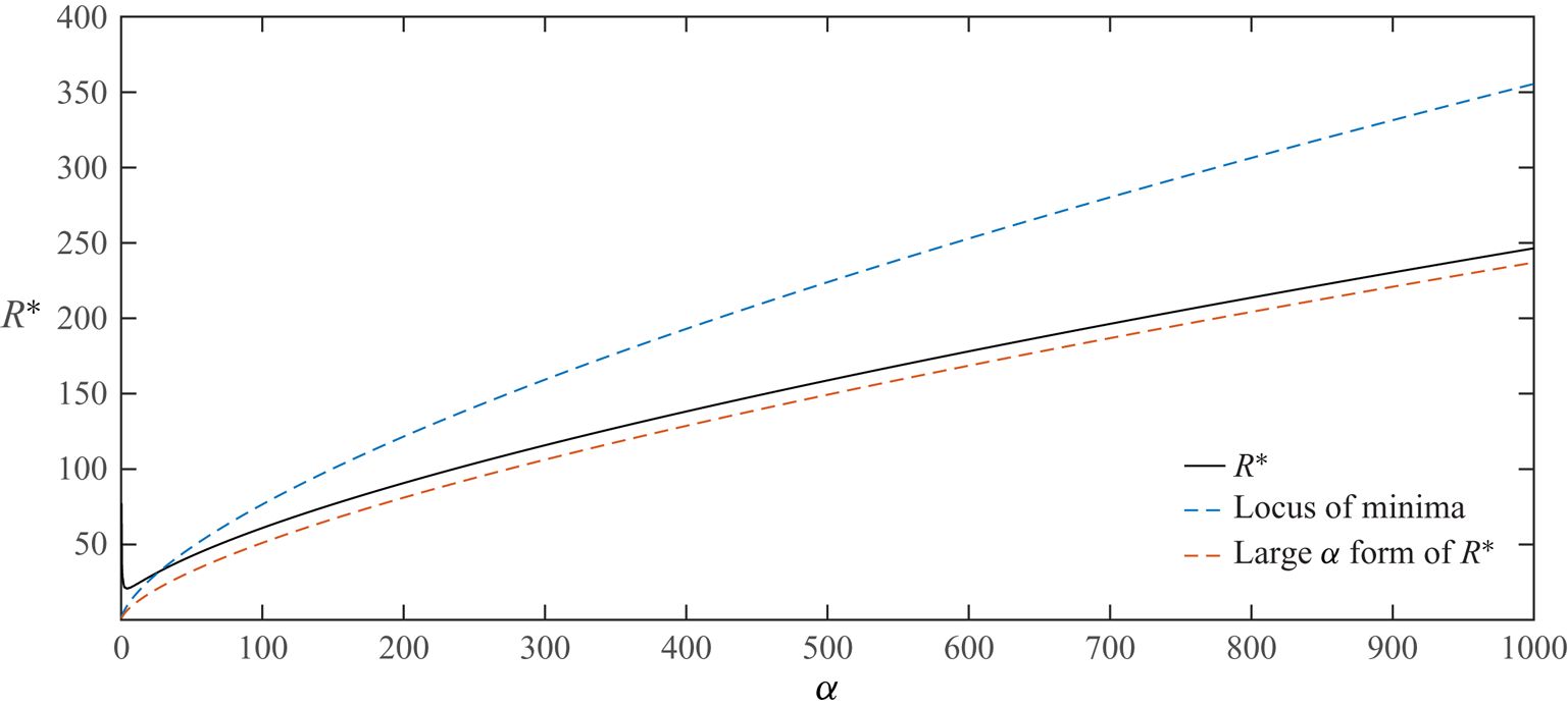
 \begin{equation} R^*\simeq \frac{\alpha^{2/3}}{ 2^{1/3}5[\textrm{Ai}'(0)]^2 }\simeq 2.37 \alpha^{2/3}. \end{equation}
On the other hand, the locus of the minima on the different neutral curves found from (4.3) noting that  $N={\alpha }/{\sqrt {2}}$ is
 \begin{equation} R^*\simeq \frac{3\alpha^{2/3}}{ 2^{1/3}10[\textrm{Ai}'(0)]^2 }\simeq 3.55 \alpha^{2/3}. \end{equation}
Figure 4 shows the variation of the lowest value of  $R^*$ over all
  $N$ as a function of
  $\alpha$. Also shown are the two asymptotic forms (4.5) and (4.6). Suppose figure 3 is extended to large
  $\alpha$ and at any
  $\alpha$ the lowest
  $R^*$ over
  $N$ is traced out as
  $\alpha$ varies, then that curve has (4.5) rather than (4.6) as asymptote.

Figure 3. (a) The neutral curves in the  $R^*-\alpha$ plane for the first five modes in the two-dimensional roughness case. In (b),
  $R^*_c$, the minimum value of
  $R^*$ over
  $\alpha$, for the first fifteen modes is shown.


It is interesting to note that, although the instability we describe here satisfies a system closely related to that satisfied by a Taylor–Görtler instability, the left-hand and right-hand branch structures here scale differently from those found in Taylor–Görtler flows. It is also important to note that the streamwise vortex in the core given by (3.6) is independent of  $\alpha$ and depends only on the azimuthal mode number
  $N$. Thus the streamwise vortex instability induced by the wall waviness occurs at a wall amplitude which depends on the wall wavelength but the structure of the vortex is independent of that wavelength.
The prediction of the  $N=3$ mode as the most dangerous is consistent with the results of Loh & Blackburn (Reference Loh and Blackburn2011) who found that, except at relatively large wall amplitudes, the
  $N=3$ mode is the most dangerous mode. Note also that the axisymmetric mode found by Cotrell et al. (Reference Cotrell, McFadden and Alder2008) is significantly less unstable than the modes considered here or in Loh & Blackburn (Reference Loh and Blackburn2011). It should also be noted that axisymmetric modes cannot be supported by the VWI type of interaction we have considered here. We presume the axisymmetric mode is associated with regions of recirculation which appear in the wave troughs as
  $\epsilon$ increases. The asymptotic description of that mode therefore requires a solution of the interactive problem which develops when
  $\epsilon$ is of size
  $R^{-({1/3})}$. However, for a given small wall amplitude
  $\epsilon$, the VWI mode considered here becomes unstable at Reynolds numbers of order
  $\epsilon ^{-({3}/{2})}$ whereas the two-dimensional mode would not become unstable until
  $R$ is
  $O(\epsilon ^{-3})$. Hence, it appears that axisymmetric modes occur only in a regime where the non-axisymmetric ones considered here are massively unstable so that the flow is likely turbulent in that regime.
The dependence of the critical Reynolds number on  $\epsilon$ is found by inverting (3.32). For the most dangerous mode the
  $R-\epsilon$ dependence is therefore given by
 \begin{equation} R=\frac{[2R^*]^{{3}/{4}}}{\epsilon^{3/2} [3 \vert{\log \epsilon}\vert]^{3/4}}+\cdots\approx \frac{7.16}{\epsilon^{3/2} \vert{\log \epsilon}\vert^{3/4}}. \end{equation}
We will compare the above prediction with the results of Loh & Blackburn (Reference Loh and Blackburn2011) later when we discuss the relevance of our two- and three-dimensional predictions with previous work.
Figure 5 shows contours of the streamfunction for the roll flow  $(U,V)$ in the
  $r$–
$r$– $\theta$ plane and contours of the corresponding streak
  $W$ for the
  $N=1,2,3,4$ modes. We note that the streamwise vortex structure becomes progressively concentrated near the pipe wall as the azimuthal wavenumber
  $N$ increases. The roll structure shown for the
  $N=3$ mode is in good agreement with figure 5 of Loh & Blackburn (Reference Loh and Blackburn2011).

Figure 5. The streamwise vortex disturbance field for the two-dimensional roughness cases. The left-hand column shows contours of constant values of the streamwise velocity component  $W$. The right column shows the streamlines in the
  $r$–
$r$– $\theta$ plane for the roll flow
  $(U,V )$ given by (3.9) for the first five modes, i.e. modes
  $N=1,2,3,4,5$. Note that the contours are independent of
  $\alpha$.
Our analysis so far has been for the case of a single streamwise harmonic, we now show how the analysis is readily extended to more general roughness shapes. Suppose then that the pipe is defined in cylindrical polar coordinates  $(r, \theta , z)$ by
 \begin{equation} r=1+\epsilon f( z), \end{equation}
where the function  $f( z)$ is periodic in
  $z$ with period
  ${ 2 {\rm \pi}}/{\alpha }$ and satisfies
  $f_{min}=-1, f_{max}=1$. We write
 \begin{equation} f(z)=\sum_{n={-}\infty}^{\infty} f_n \exp({\textrm{i} n \alpha z}), \end{equation}
with  $f_0=0$. The coefficients
  $f_n$ for a particular pipe could be calculated by scanning the pipe surface; see for example Mughal & Ashworth (Reference Mughal and Ashworth2013) for a discussion of boundary-layer instabilities in flows over rough surfaces.
The instability mechanism we have described is driven by the interaction of the basic Poiseuille flow and the axial component of the streamwise vortex both modified by the wall undulations. Thus, at the order considered above, the contributions from interactions involving different streamwise wavenumbers is negligible. Therefore, in the more general case, (4.1) is replaced by a sum over all the axial wavenumbers. It follows that the neutral value of  $R^*$ for the more general roughness shape is given by
 \begin{equation} R^*= \frac{ (N+1)(N+2)} { 2^{1/3}5 \alpha^{4/3} N^2 [\textrm{Ai}'(0)]^2 \displaystyle\sum_{m={-}\infty}^{\infty}\frac{ f_m^2 m^{4/3} } {N^2+ m^2 \alpha^2}}. \end{equation}
Because the  $\alpha$ dependence of
  $R^*$ is now embedded in the summation we cannot predict the dependence of
  $\alpha$ on
  $N$ for the most unstable mode. Therefore, we cannot infer that the most dangerous azimuthal mode is the
  $N=3$ mode and, even when it is, the most dangerous streamwise wavenumber is not
  $3\sqrt {2}$. However, the form of the terms within the summation means that, even for roughness elements having step-function-like discontinuities for which the Fourier coefficients will decrease like
  $m^{-1}$, the dominant contribution will correspond to that from
  $m=1$ and so it is likely that the most dangerous mode will still have
  $N = 3$. For definiteness we now consider the roughness elements shown in figure 6.

Figure 6. Different types of roughness elements to be considered. (a,b) shows a square wave and pulse function, (c,d) shows sawtooth and triangular walls and (e,f) shows rectified sine wave and sine wave walls.
Having calculated the Fourier coefficients for each of the roughness shapes we calculate  $R^*$ as a function of
  $\alpha$ for
  $N=1,2,3,4,5,\ldots$. We found that, in fact, the
  $N=3$ mode remained the most dangerous mode in each case. Figure 7 shows the neutral curves for the roughness elements of figure 6. We see that the square wave is apparently the most dangerous shape and it leads to a critical value of
  $R^*$ which is about one half of its value for the single sine wave. In terms of
  $R-\epsilon$ the condition for instability the curves in figure 7 predict instability when
 \begin{equation} R> \frac{\phi}{\epsilon^{3/2} \vert{\log \epsilon}\vert^{3/4}}, \end{equation}
where  $4.59<\phi <10.9$ so that for a given small wall amplitude the shape of roughness likely can make about a factor of 2 difference in the critical Reynolds number. Once again we stress that the streamwise vortex structure is independent of the wavenumber
  $\alpha$ and so independent of the roughness shape and therefore the modes are still as indicated in figure 5.

Figure 7. The neutral curves for the most dangerous modes (all  $N=3$) for the two-dimensional roughness shapes shown in figure 6.
5. Three-dimensional roughness
If the azimuthal wavenumber of the roughness is non-zero, then there is not an analytical expression for  $R^*$ available and we must solve the eigenvalue problem (3.37) numerically. Note that (3.37) corresponds to the most general form of
  $\theta$ dependence for the streamwise vortex and, based on our results for the two-dimensional problem, we anticipate that for given values of
  $\alpha$ and
  $N$ there will be an infinite discrete spectrum of eigenvalues
  $R^*$. Here our interest is primarily in the most dangerous mode for the given values of
  $\alpha$ and
  $M$. The eigenvalue problem was solved using MATLAB. Negative values of
  $R^*$ are not physically relevant and so we are interested in the largest positive value of the eigenvalue
  ${1}/{R^*}$ which therefore, for given values of
  $\alpha , M$, gives instability at the least value of
  $R^*$. The eigenvalue problem was solved for both the even and odd modes and results for
  $M=1,2,3,4,5$ are shown in figure 8. We see that in both cases the
  $M=1$ roughness is the most unstable. However, by comparison with figure 3 we conclude that two-dimensional roughness is more unstable than three-dimensional roughness.

Figure 8. (a,b) The neutral curves for the even and odd modes in the  $\alpha -R^*$ plane for the three-dimensional roughness case with
  $M=1,2,3,4,5$.
We stress that in spite of the relative similarity between the results shown in figures 3 and 8 they are conveying different information. Figure 3 shows the neutral curves for the first five neutral modes for two-dimensional roughness whilst figure 8 shows the dependence of  $R^*$ on
  $\alpha$ for the most unstable odd and even modes for different values of
  $M$. We stress that for the three-dimensional case we do not specify an azimuthal wavenumber for the disturbance. Instead we have a sequence of eigenvalues
  $R^*$ with eigenfunctions distributed amongst the different values of
  $N$. Moving along any of the neutral curves in figure 8 the dominant Fourier term in the decomposition of the disturbance changes and there can be many slightly less unstable modes bunched in the vicinity of the most dangerous one. Thus for the even mode, the most unstable mode can jump to one with a quite different Fourier decomposition as
  $\alpha$ varies. The result of the jump in modes means that if figure 8 is enlarged discontinuities in slope along the curves can be seen where the jump occurs. In addition we observe that the most dangerous even mode for
  $M=4$ jumps discontinuously near
  $\alpha =14.5$. A careful investigation around that point shows that the branch to the left of the discontinuity has increasing slope before turning and developing for decreasing
  $\alpha$ as a less unstable mode. By contrast the right-hand part of the
  $M=4$ curve continues above both branches of the left-hand part of the curve as
  $\alpha$ decreases and so ceases to be the most unstable mode as
  $\alpha$ is decreased below
  $15.5$.
Figure 9 shows the variation of  $R^*_c$, the minimum value of
  $R^*$ over
  $\alpha$, for both the even and odd modes, we see that in each case the odd mode is the most unstable. That property holds for all higher values of
  $M$ investigated but not shown here. Since the odd mode is always the most unstable we will for the most part concentrate on that mode below.

Figure 9. The variation of  $R^*_c$ the minimum of
  $R^*$ over
  $\alpha$ for the first ten values of
  $M$ for the odd (red symbol) and even (blue symbol) modes.
The calculations uncovered significant differences between the eigenfunctions associated with the most unstable odd and even modes calculated from the more general form (3.6) and the simplified form where the Fourier decomposition of the disturbance involves only multiples of the roughness wavenumber  $M$. However, for the odd mode we find that the most unstable mode from the constrained expansion coincides with that from the full expansion. Hence the Fourier decomposition of the most dangerous odd mode contains only integer multiples of
  $M$. We see from (3.25)–(3.31) that it is
  $2M\theta$ rather than
  $M\theta$ that appears in the disturbance equations, therefore the odd mode corresponds to a
  $1/2$ subharmonic.
Our calculations show that, in contrast to the odd mode, the even mode has a more complex structure and in most instances the Fourier decomposition of the most unstable even mode contains non-integer multiples of the roughness wavenumber  $M$. In fact we find that for larger values of
  $M$ the even mode is typically dominated by the
  $M \pm 1$ Fourier components. The latter modes have almost equal and opposite values so the streamwise velocity disturbance for large
  $M$ is proportional to
  $\sin M\theta \sin \theta$ and the mode is more correctly described as a sideband instability; see for example Eckhaus (Reference Eckhaus1965).
If we choose a value for  $M$ and compute the values of
  $R^*$ corresponding to the most unstable odd and even modes at increasing values of
  $\alpha$ we find that, as shown in figure 8,
  $R^*$ will vary like
  $\alpha ^{2/3}$ for
  $\alpha$ large. In fact our calculations showed that in the large
  $\alpha$ limit the most unstable odd and even modes have the asymptotic form (4.5) found earlier for the two-dimensional case. Thus when the streamwise variation of the roughness varies much more quickly than the azimuthal variation the most unstable mode occurs at the same value of
  $R^*$ as the two-dimensional case. Thus if figure 8 is extended to higher values of
  $\alpha , M$ the neutral curves would have the curve
  $R^*\simeq 2.37 \alpha ^{2/3}$ as an envelope.
If we constrain the disturbances to contain only multiples of  $M$ in their Fourier decompositions then we must solve the simplified eigenvalue problem (3.40). For the odd mode that procedure invariably gives the same most unstable mode as the more general expansion. For the even mode that is not the case and the most unstable mode does not come from the simplified problem. However, the most unstable odd and even modes of the constrained problem once again adopt the asymptotic form (4.5) for large
  $\alpha$, but we stress that all solutions with increasing
  $\alpha$ do not have that property.
By neglecting the terms of order  ${1}/{M}$ in (3.38a,b) we can solve for the asymptotic eigenrelations given by (3.42a,b) and (3.43a,b). However, we stress that the resulting asymptotic form assumes the Fourier decomposition of the disturbance involves only multiples of
  $M$ and so does not necessarily connect with the most unstable even or odd mode at lower
  $\alpha$. Figure 10 shows the variations of
  $R_e^+, R_o^+$ for a range of values of the scaled wavenumber
  $\alpha ^+$. We see that the predicted values have the same asymptotic form for large
  $\alpha ^+$; in fact numerically it was found that, as can be anticipated from the above discussion,
  $R_e^+, R_o^+$ both behave like
  $2.37 [\alpha ^+]^{2/3}$ for large
  $\alpha ^+$. Figure 10 shows that in the high
  $M$ limit the odd mode remains the most unstable with instability occurring first at
  $(\alpha ^+,R^+_{ o})=(2.91,9.03)$ whilst the even mode becomes unstable when
  $(\alpha ^+,R^+_{ e})=(3.75,10.04)$ We note also that the even mode has a single minimum whilst the odd mode has two.

Figure 10. The odd and even functions  $R^+_{ e}, R^+_{ o}$ for a range of values of
  $\alpha ^+$.
Figure 11 shows a comparison of the  $\alpha -R^*$ dependence of the most unstable odd and even modes found by solving the full eigenvalue problem with the asymptotic forms (3.42a,b) and (3.43a,b) using the data of figure 10. We see that at large
  $M$ the most unstable even and odd mode neutral curves are remarkably close together over the whole range of
  $\alpha$. The asymptotic prediction of the curve for odd mode curve agrees almost perfectly with the full solutions, by contrast the asymptotic prediction for the even mode agrees only at large
  $M$. This is because the asymptotic solutions we constructed assumed the Fourier decomposition of the disturbance field involved only multiples of
  $M$. For the odd mode that property is shared by the solution of the full problem assuming no special structure. However, the even mode solution of the full problem does not share the same special structure. Since the odd mode is always the most unstable we do not pursue alternative large
  $M$ asymptotic descriptions of the modes here.

Figure 11. Comparison between odd and even modes for  $M=100,200$ with the large
  $M$ asymptotic result for the odd mode.
Now, let us discuss the velocity fields associated with the even and odd modes. Figures 12 and 13 show the contours of the streamfunction and axial velocity of the most dangerous odd and even modes for  $M=1,2,3,4,5$. In each case the eigenfunctions are evaluated at the minimum points of the neutral curves. We see that the flow fields tend to become more regular at the higher values of
  $M$; indeed the disturbance field is then similar to the two-dimensional case. This is because the critical configuration occurs at progressively higher values of
  $\alpha$ as
  $M$ increases and thus takes on the more regular properties found in the two-dimensional case.

Figure 12. Contours for the axial velocity (a,c,e,g,i) and streamwise vortex streamfunction (b,d,f,h,j) for the even modes at the minima in figure 8. Results are shown in the order  $M=1,2,3,4,5$ from top to bottom.

Figure 13. Contours for the axial velocity (a,c,e,g,i) and streamwise vortex streamfunction (b,d,f,h,j) for the odd modes at the minima in figure 8. Results are shown in the order  $M=1,2,3,4,5$ from top to bottom.
The results found above show that for three-dimensional roughness the odd mode is always more unstable than the corresponding even one, but both are less unstable than the most dangerous mode for the case of two-dimensional roughness. Thus three-dimensional roughness with  $M=1$ gives instability whenever
  $R^* >26.02$ whereas two-dimensional roughness gives instability when
  $R^*> 20.70$.
For given small values of  $\epsilon$ the corresponding neutral values of
  $R$ are calculated as indicated in (4.7). Figure 14 shows the
  $\alpha -R$ dependence for the most dangerous two and three-dimensional roughness cases. Also in the figure we have plotted the results of Cotrell et al. (Reference Cotrell, McFadden and Alder2008) who investigated the instability of two-dimensional roughness to two-dimensional disturbances. We see that such modes are significantly less unstable. In addition the numerical results of Loh & Blackburn (Reference Loh and Blackburn2011) on two-dimensional roughness are shown for
  $\alpha =4,6$. The latter two values are comparable to the critical values of
  $\alpha$ we obtained for the two and three-dimensional roughness cases. The results are increasingly consistent with the asymptotic results as
  $\epsilon$ decreases and show the same trend as the asymptotic results until
  $\epsilon$ is about
  $0.35$ where the full numerical calculations give increasing values of
  $R$ as
  $\epsilon$ decreases.

Figure 14. Comparison of theoretical predictions with previous numerical work and experiment.
Figure 14 also includes experimental results taken from figure 10 of Kandlikar (Reference Kandlikar2008). The results indicated by the blue and red crosses at each  $\epsilon$ correspond to measurements in water and air respectively. The agreement with the asymptotic predictions is excellent, this might be fortuitous since the full numerical results of Loh & Blackburn (Reference Loh and Blackburn2011), which one might expect to be in better agreement with experiment, are less consistent with experiments.
6. The limits of small and large scale roughness
6.1. Small scale roughness and a universal criterion for roughness induced instability
In the previous sections we have described the instability of Hagen–Poiseuille flow caused by wall roughness varying on the same length scale as the pipe radius. We have shown that instability will occur when
 \begin{equation} R \ge \frac{[2R^*(\alpha, M)]^{{3}/{4}}}{\epsilon^{3/2} [3 \vert{\log \epsilon}\vert]^{3/4}}+\cdots, \end{equation}
with, in the most dangerous configurations,  $R^*=20.7$ and
  $26.02$ for two and three-dimensional roughness respectively. In both the two and three-dimensional cases in the limit of large
  $\alpha$ the lowest value of
  $R^*$ at which instability occurs has the asymptotic dependence
  $R^* \simeq 2.37 \alpha ^{2/3}$. However, as indicated in figure 8, the rate at which that limit is approached in the three-dimensional case depends on
  $M$.
$M$.
It is useful at this stage to express (6.1) in an alternative form. In dimensional form the radius of the pipe can be taken as  $a(1+2\epsilon \cos M \theta \cos {\alpha z^*}/{a})$ where
  $z^*$ is the dimensional length in the streamwise direction. The dimensional wavelength of the radius variations in the streamwise direction
  $b$ and the wave height
  $h$ are given by
 \begin{equation} b=\frac{2 {\rm \pi}a}{\alpha},\quad h=2 \epsilon a. \end{equation}
If the maximum streamwise velocity in the straight pipe is  $U_0$ then the friction velocity
  $u_{\tau }$ is given by
  $u_{\tau }=\sqrt {{\nu U_0}/{a}}$. We define
  $R_b$, a Reynolds number based on the streamwise wall wavelength
  $b$ and the frictional velocity, by writing
 \begin{equation} R_b=\frac{u_{\tau}b}{\nu}=\frac{b\sqrt{R}}{a}. \end{equation}
Thus, since  ${a}/{h}\gg 1$, we can write (6.1) in the form
 \begin{equation} R_b \ge \frac{b}{a^{1/4} h^{3/4}} \left(\frac{8R^*(\alpha, M)}{3 \log \dfrac{a}{h}} \right)^{3/8}. \end{equation}
Now, we suppose that the roughness operates on a smaller length scale, that would likely be the case if it is a result of manufacturing imperfections rather than ‘designed roughness’. If the roughness length scales in the streamwise and azimuthal directions decrease at the same rate then we need to consider the structure of  $R^*(\alpha , M)$ in the limit
  $\alpha , M \rightarrow \infty ,$ with
  ${\alpha }/{M}$ held fixed. This is precisely the regime discussed earlier in § 3; see the discussion around (3.40) and (3.42a,b). We recall that for modes having energy only in Fourier modes corresponding to integer multiples of
  $M$ the even and odd function
  $R^+_o, R^+_e$ are as shown in figure 10. We now consider only the odd mode since we found that it is always the most unstable and can be described by the constrained Fourier decomposition. Thus if we concentrate on the odd mode we replace
  $R^*$ in (6.4) by
 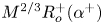 $M^{2/3}R_o^+(\alpha ^+)$ where
  $\alpha =\alpha ^+M$ to give the condition
 \begin{equation} R_b \ge \frac{bM^{1/2}}{a^{1}/{4} h^{3/4}} \left( \frac{8R^+_o(\alpha^+)}{3 \log \dfrac{a}{h}} \right)^{3/8}. \end{equation}
This is the condition for instability when the roughness is on a length scale that is small compared to the pipe radius with  $R^+_o$ given in figure 10; the minimum occurs when
  $R^+_o=9.03$. Now suppose that the roughness length scale in the axial direction is short compared to that in the azimuthal direction. In that case
  $\alpha^+\gg1$ and
  $R^+_o\simeq 2.37( \alpha^+)^{2/3}$ and (6.5) becomes
 \begin{equation}R_b \ge \frac{3.16 \left[\dfrac{b}{h}\right]^{3/4}}{\left(\log \left[\dfrac{a}{b}\right]+ \log\left[\dfrac{b}{h}\right]\right)^{3/8}}. \end{equation}
 Thus, the condition for instability in this case depends only weakly on the pipe radius through the logarithmic term in the denominator and, if  ${a}/{b} \ll {b}/{h}$, the condition becomes
 \begin{equation} R_b \ge 3.16 \frac{\left[\dfrac{b}{h}\right]^{3/4}}{\log\left[\dfrac{b}{h}\right] ^{3/8}}. \end{equation}
This condition is now independent of the pipe radius and applies to short scale roughness varying more quickly in the streamwise direction. The condition also applies to short scale two-dimensional roughness, and being independent of the pipe radius it is a universal result which can for example be derived from the results of Hall (Reference Hall2020) for channel flows.
6.2. Roughness on a long length scale
Now let us make some observations about the situation when the streamwise variation of the roughness is on a length scale large compared to the pipe radius. We will consider only the two-dimensional case. We see from (4.1) that in the limit of small  $\alpha$
 \begin{equation} R^* \simeq \frac{C(N)}{\alpha^{4/3}}, \end{equation}
where
 \begin{equation} C(N)=\frac{ (N+1)(N+2)} { 2^{1/3} 5 \textrm{Ai}'(0) ^2}. \end{equation}
It follows that at small values of  $\alpha$ the
  $N=1$ mode is the most dangerous mode. In terms of
  $h,b$ the dimensional height and wavelength of the wall undulations, instability in the two-dimensional case thus occurs when
 \begin{equation} \frac{h}{a}>\frac{ 2\sqrt{C(1)}\left[\dfrac{b}{a}\right]^{2/3}}{(2{\rm \pi})^{2/3}R^{2/3}\sqrt{\log R}}. \end{equation}
In this limit  ${h}/{a}\ll {b}/{a}$ so that in the above formula we can replace
  $\log R$ by
  $\log [{b}/{a}]$. The authors are not aware of experimental or numerical predictions of the critical wave height
  $h$ in this parameter range. It is of interest to speculate about what the above result implies for boundary layers where there has been much interest in the effects of waves on transition, see for example Fage (Reference Fage1943) and Carmichael (Reference Carmichael1959).
In the boundary-layer case, boundary-layer growth somewhat complicates the issue but, if we assume that the left-hand branch structure  $R^* \simeq {C(N)}/{\alpha ^{4/3}}$ remains intact in the presence of non-parallel effects, we can draw some conclusions. Note that we know from Denier, Hall & Seddougui (Reference Denier, Hall and Seddougui1991) that the left-hand branch structure of Görtler vortices expected on the basis of Taylor vortex theory remains intact when non-parallel effects are taken care of.
In the boundary-layer case the appropriate Reynolds number is based on the local boundary-layer thickness rather than pipe radius  $a$. If we write the condition for instability in terms of the Reynolds number
  $R$ based on chord length scale
  $L$ then we find instability occurs when
 \begin{equation} \frac{h}{L}> \frac{F \left[\dfrac{b}{L}\right]^{2/3}}{R^{7/6}\sqrt{\log \left[\dfrac{b}{L}\right]}}, \end{equation}
where  $F$ is a constant dependent on the form of the initial disturbance. By comparison with experimental results, Fage (Reference Fage1943) arrived at the result
 \begin{equation} \frac{h}{L}> \frac{G \left[\dfrac{b}{L}\right]^{1/2}}{R^{3/2}}, \end{equation}
where  $G$ is a constant. Subsequent work by Carmichael, Whites & Pfenninger (Reference Carmichael, Whites and Pfenninger1957) and Carmichael & Pfenninger (Reference Carmichael and Pfenninger1959) was broadly in agreement with Fage's results and certainly their experiments supported the result that the critical configuration has
  ${h^2}/{b}$ a constant. By contrast (6.12) predicts
  ${h^2}/{b^{4/3}}$ is constant, whilst there is a factor
  $b^{1/6}$ different between the present results and experiments the square root of the logarithmic term in the denominator of (6.12) partially accounts for that factor. However, there is a more significant factor of
  $R^{1/3}$ power between the two equations. Nevertheless, the overall trend of the two results is consistent and it should be pointed out that (6.12) was derived on the basis of a small number of experiments on wall deformations of different shapes.
7. Conclusion
We have described a VWI instability mechanism which governs the growth of streamwise vortex perturbations induced by wall undulations. The instability is operational when the Reynolds number satisfies (6.1) or, equivalently, (6.4) in terms of the Reynolds number based on friction velocity and streamwise wall wavelength. If the radius variations are on a shorter length scale than the pipe radius then the condition simplifies to (6.5). Moreover, when azimuthal variations are slow compared to the axial ones, or when they are absent, (6.5) can be reduced to (6.7) which is independent of the pipe radius. Therefore, (6.7) is a universal result which applies to any fully developed pipe or channel flows. It should be noted that the instability mechanism can only occur when axial variations are present so that azimuthal radius variations alone cannot induce the VWI mechanism. If only azimuthal perturbations are present the basic state is a unidirectional flow depending on the two variables in the plane perpendicular to the axis. In the absence of the mechanism described here instability will likely require wall amplitudes comparable with the radius of the pipe.
Our results are broadly consistent with the numerical results of Loh & Blackburn (Reference Loh and Blackburn2011) and predict instability before the axisymmetric mode of Cotrell et al. (Reference Cotrell, McFadden and Alder2008) becomes unstable. The latter authors also argue that instability is only possible when the wall undulations are sufficiently large to cause reversed flow in the troughs of the pipe wall. For small amplitudes reversed flow only occurs in the interactive regime  $\epsilon =O(R^{-({1/3})})$ which would mean that for a given small value of
  $\epsilon$ instability occurs only when
  $R>{d}/{\epsilon ^3}$, however, the curve fit given by Cotrell et al. (Reference Cotrell, McFadden and Alder2008) has instability when the Reynolds number is
  $O(\epsilon ^{-1})$. The reason for the expected scaling and the curve fit of the latter authors differing is perhaps because their results were at values of
  $\epsilon$ too large for the small
  $\epsilon$ asymptotic to be a good approximation. However, it should also be noted that Cotrell et al. (Reference Cotrell, McFadden and Alder2008) reported that, in an axisymmetric pipe, three-dimensional modes are less unstable than two-dimensional ones. That result is at odds with our results and those given by Loh & Blackburn (Reference Loh and Blackburn2011).
The VWI mechanism described here can be extended to the situation when the axial undulations contain a number of Fourier modes. We have only investigated the more general situation when the wall undulations are axisymmetric but the method used in § 4 is readily extended to the more general case. For the cases investigated in § 4 we found that step function roughness was the most destabilising, but even then the critical value of  $R^*$ needed for instability is only about one half of its value for the pure sine wave case so the actual shape of the roughness appears not to be crucial. The roughness we considered also contained a single Fourier mode in the
  $\theta$ direction, the more general case could be considered and in that case the matrix
  ${{\boldsymbol{\mathsf{A}}}}$ in (3.37) becomes full.
There is an important difference in our results for two and three-dimensional wall undulations. In the first case we found that there is an infinite set of unstable modes and that the  $N=3$ azimuthal mode is the most dangerous one with the corresponding wall undulation wavenumber given by
  $\alpha =3\sqrt {2}$. Interestingly the fact that the critical Reynolds numbers for the
  $N=2,3,4,5$ modes are quite close together is consistent with exact coherent structure solutions in smooth pipes; see Eckhardt et al. (Reference Eckhardt, Schneider, Hof and Westerweel2007) or the discussion in Wedin & Kerswell (Reference Wedin and Kerswell2004). However, it should be noted that the exact coherent structures we refer to support waves which travel downstream with a non-zero speed whereas the waves implicated in the instability mechanism discussed here are stationary. We presume that the similar importance of the
  $N=2,3,4,5$ modes in what are distinct physical problems is that those azimuthal modes decay at similar rates in smooth pipes. In the present problem the wall undulations destabilise these modes whereas in the exact coherent structure context those streamwise modes are reinforced by the VWI mechanisms within their critical layers. It should also be pointed out that the
  $N=1$ mode which is known from Schmid & Henningson (Reference Schmid and Henningson1994) to be the most rapidly growing transient mode is significantly more stable than the
  $N=2,3,4,5$ modes and plays a less prominent role in the exact coherent structure context.
In the case of three-dimensional undulations we computed the most dangerous mode which now has energy distributed in a number of azimuthal wavenumbers. We found that wall undulations with  $M=1$ give the most unstable even and odd modes. We found that, in general, the most dangerous mode, the odd one, has energy only in modes corresponding to integer multiples of
  $M$. At finite values of
  $\alpha$ we found that two-dimensional roughness was always more unstable than three-dimensional roughness. However, in the limit of short scale roughness with
  $M, \alpha$ large we found that at leading-order instability occurred at the same
  $R^*$ for the two and three-dimensional cases. The conclusion is of course that roughness in the form of pipe radius variations need only occur at quite tiny amplitudes in the axial direction to produce instability.
Acknowledgements
The authors wish to thank the referees for their helpful comments on the first draft of this paper.
Funding
This work was supported by the Australian Research Council (ARC DP 170104703).
Declaration of interests
The authors report no conflict of interest.
Appendix A. Evaluation of the elements of the matrix  ${{\boldsymbol{\mathsf{A}}}}$

Here, we will derive expressions for the constants  $a_N, b_N, c_N, d_N$ introduced in § 3 for even modes where streamwise velocity component of the vortex is an even function of
  $\theta$. In the first instance we suppose that
  $M\ne 0.$ For convenience, we define a sequence
  $\lambda _N, N=0,\pm 1,\pm 2,\ldots$ by first expanding
  $\lambda (\theta )={W'(1, \theta )}$ in the form
 \begin{equation} \lambda=\sum_{N=1}^{\infty} \lambda_N \cos N\theta \end{equation}
and then taking  $\lambda _N=0, N<1$. The first step is to solve for
  $S(\theta )$ which satisfies (3.25). By substitution it is easily seen that
 \begin{gather} S(\theta)=\sum_{N=1}^{\infty}\alpha_n \cos M \theta \cos N \theta+\beta_N \sin M \theta \sin N \theta, \end{gather}
 \begin{gather}\frac{\alpha_N}{\lambda_N}=\hat{\alpha}_N=\frac{ {5}{ }(N^2+M^2+\alpha^2)-\dfrac{ {9}{ }M^2N^2}{\alpha^2+M^2}} {(N^2+M^2+\alpha^2)^2-4M^2N^2 }, \end{gather}
 \begin{gather}\frac{\beta_N}{\lambda_N} =\hat{\beta}_N= \frac{(N^2+M^2+\alpha^2)\hat{\alpha}_N- {5}{ } }{2MN}. \end{gather}
Using the above form for  $S(\theta )$ we can then compute the functions
  $S'(\theta )\cos M\theta , S (\theta )$ appearing in (3.22) to give
 \begin{gather} Q_1(\theta)= \frac{1}{\mu}\sum_{N=1}^{\infty}[a_N \lambda_N+b_N \lambda_{N-2M}+c_N\lambda_{N+2M}+d_N\lambda_{2M-N}]\sin N \theta \end{gather}
 \begin{gather}\frac{2a_N}{\alpha^2+M^2}={-}( { {\alpha}} ^2+3M^2)(M \hat{\beta}_N-N \widehat{{\alpha}}_N)-2M {\alpha}^2 \widehat{{\beta}}_N \end{gather}
 \begin{gather}\frac{4b_N}{\alpha^2+M^2}={-}(\hat{\alpha}_{N-2M}-\hat{\beta}_{N-2M})[(M-N)(\alpha^2+3M^2)+2M\alpha^2], \end{gather}
 \begin{gather}\frac{4c_N}{\alpha^2+M^2}={-}(\hat{\alpha}_{N+2M}+\hat{\beta}_{N+2M})[-(M+N)(\alpha^2+3M^2)-2M\alpha^2], \end{gather}
 \begin{gather}\frac{4d_N}{\alpha^2+M^2}={-}(\hat{\alpha}_{2M-N}+\hat{\beta}_{2M-N})[(M-N)(\alpha^2+3M^2)+2M\alpha^2]. \end{gather}
Similarly, we can show that
 \begin{equation} Q_2(\theta)=\frac{1}{\mu}\sum_{N=1}^{\infty} [e_N\lambda_N+ f_N\lambda_{N-2M}+g_N \lambda_{N+2M}+h_N\lambda_{2M-N}]\sin N \theta, \end{equation}
where
 \begin{equation} \left.\begin{gathered} e_N={-}\frac{3}{4}M^2N,\quad f_N=h_N=\frac{3M}{8}(6\alpha^2+MN-4M^2),\\ g_N={-}\frac{3M}{8}(6\alpha^2-MN-4M^2). \end{gathered}\right\} \end{equation}
We then define
 \begin{gather} A_N={-}\frac{2^{{4}/{3}} \alpha^{4/3}\textrm{Ai}'^2(0)}{ (\alpha^2+M^2)^2}(a_N+e_N), \end{gather}
 \begin{gather}B_N={-}\frac{ 2^{4/3} \alpha^{{4}/{3}}\textrm{Ai}'^2(0)}{ (\alpha^2+M^2)^2}(b_N+f_N), \end{gather}
 \begin{gather}C_N={-}\frac{ 2^{4/3} \alpha^{{4}/{3}}\textrm{Ai}'^2(0)}{ (\alpha^2+M^2)^2}(c_N+g_N), \end{gather}
 \begin{gather}D_N={-}\frac{ 2^{4/3} \alpha^{{4}/{3}}\textrm{Ai}'^2(0)}{ (\alpha^2+M^2)^2}(d_N+h_N). \end{gather}
The matrix  ${{\boldsymbol{\mathsf{B}}}}$ introduced in § 3 has then all elements zero except for:
(a) The main diagonal has
$B_{NN}=A_N, N\ne M$ and $B_{MM}=A_{MM}+D_{MM}$.(b) The
$(2M+N,N)$ element for $N=1,2,\ldots$ is $C_N$.(c) The
$(2M+N, N)$ element for $N=1,2,\ldots$ is $B_N$.(d) The
$(N, 2M-N)$ element for $N=1,2,\ldots ,2M-1$ is $D_N$.
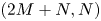


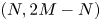

In the case  $M=0$ the matrix
  ${\boldsymbol{\mathsf{B}}}$ has all off-diagonal elements zero and the diagonal element
  $B_{NN}$ is given by
 \begin{equation} B_{NN}=\frac{2^{4/3}N \alpha^{4/3}\textrm{Ai}'^2(0) }{\alpha^2+N^2}. \end{equation}


