


1.0 INTRODUCTION
Gravity gradient satellites have long been a practical solution for Earth observation and Earth science missions. The gravity gradient satellite is generally formed by a main-sat and a sub-sat (detector) joined by a coilable mast, the length of which is within the range of 2–5m. In order to explore the global distribution of spatial physical parameters, the gravity gradient microsatellite is subject to the problem of the orbital transfer. Normally, conventional orbital transfers can be utilised, such as the Hohmann orbital transfer or the bielliptical orbital transfer. Whereas, impulse orbital transfers have several limitations; for example, the impulse thruster may lead to the vibration of the coilable mast, which is adverse to the attitude control of the gravity gradient microsatellite. With the progress of the micro-thrust technology, a small, continuous and constant thrust becomes a practical and effective method, which possesses merits such as low control requirements, high safety, and repeatability.
In orbital transfer, in order to save on the cost, power, weight and complexity of the system, a magnetorquer is normally adopted to provide the control torque. Several control methods have been developed for the attitude acquisition, manoeuvre and stabilisation of magnetic actuated satellites during the last decades(Reference Burton, Rock, Springmann and Cutler1–Reference Walker and Putman5). The well-known B-dot control law was proposed early in 1972(Reference Rodriquez-Vazquez, Martin-Prats and Bernelli-Zazzer6). In addition, because the magnetic control torque lies in a two-dimensional plane orthogonal to the magnetic field, the relevant research is mainly focused on the stability analysis of magnetic control laws. The local asymptotic stability is easily addressed(Reference Ovchinnikov, Roldugin, Penkov, Tkachev and Mashtakov7–Reference Huang and Yan9), and the global asymptotic stability is proved to be possible when the magnetic field variation is sufficient along a complete orbit(Reference Zhou, Huang, Wang and Sun10–Reference Sofyali, Jafarov and Wisniewski12).
In spite of a number of studies in the aforementioned literature, the control performance is still greatly influenced by the magnetic constraint. In this article, the unique features of the proposed tracking control are mainly shown in two aspects: (1) According to the analysis of the combined forcing action of the gravity and the constant thrust, an expected attitude trajectory is proposed. Based on the expected trajectory, the torque produced by the thrust can be compensated by the torque produced by the gravity; hence, the trajectory is stable and reduces the energy consumption of the controller. (2) An auxiliary compensator is proposed, and a sliding mode control method, based on the compensator, is presented. Due to the boundedness of the control error, the magnetic constraint compensator is dissipative; as the sliding surface maintains at zero, attitude angles realise the tracking of the expected attitude trajectory, and the system is asymptotically stable.
In this paper, in Section 2.0, the problem is formulated; in Section 3.0, the dynamic model is established; in Section 4.0, an expected attitude trajectory is derived, and a method of the magnetic sliding mode control is presented; in Section 5.0, a numerical case is studied to demonstrate the effectiveness of the proposed control.
2.0 PROBLEM FORMULATION
The study on the magnetic attitude tracking control is mainly applied to a gravity gradient microsatellite in orbital transfer, which can be adopted for the environment exploration of the atmosphere or the ionised layer. In order to obtain the large-scale three-dimensional spatial environment data, the gravity gradient microsatellite is subjected to the problem of the orbital transfer.
In orbital transfer, a continuous thrust is imposed on the gravity gradient microsatellite (Figure 1), which is completely different from the traditional gravity gradient microsatellite in a Keplerian orbit. When the torque generated by the thrust is close to the gravity gradient torque, the equilibrium positions of attitude angles will be decided by the geocentric distance, the thrust, and the length of the coilable mast. Besides, as the thrust is positioned along a settled direction, the bifurcation and resonance phenomena may occur. It might arouse not only the attitude disorder, but also the strong vibration of the coilable mast.
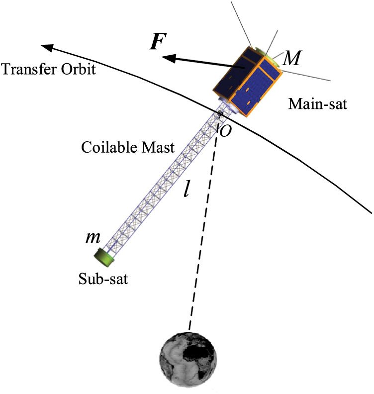
Figure 1. The description of the gravity gradient microsatellite.
In order to inhibit the pendular motion of the gravity gradient microsatellite in orbital transfer, an effective attitude tracking controller should be implemented. Besides, in order to reduce cost, power, weight and system complexity, a magnetorquer can be installed in the main-sat. Considering that a constant thrust along the transversal direction can be applied to the orbital transfer between two circular low Earth orbits (LEOs)(Reference Zhu and Wang13), a case of the transversal orbital transfer is mainly studied in the paper.
3.0 DYNAMIC MODEL
3.1 Coordinate frames
Let Ex’y’z’ be the geocentric inertial frame. Its origin E is the mass center of the Earth. The axis Ex’ points to the first Aries point, the axis Ey’ is in the equatorial plane and the coordinate system is right-hand oriented.
Subsequently, let Oxyz be the orbital frame with the origin at the mass center of the microsatellite O. The Oz axis points to the mass center of the Earth E, the Ox axis is normal to the Oz axis in the orbital plane and points along the direction of increasing polar angle u and the coordinate system is right-hand oriented.
Afterwards, let  $Ox_oy_oz_o$ be the original frame with the origin at the mass center O. The axes are assumed to coincide with the microsatellite’s principal inertia axes.
3.2 Attitude dynamics
Because the gravity gradient microsatellite is regarded as a rigid body, the attitude dynamic equation can be expressed as
 \begin{equation}{{\bf{I}}{\dot{\bf\omega}}} = {\bf{f}}\left( {{{\bf\omega}},t} \right) + \Delta {{\bf{f}}}\left( {{\bf\omega},t} \right) + \Delta {\bf{d}}\left( t \right)+ {\bf{M}}_C\end{equation}
where  ${{\bf{f}}}\left( {{{\bf\omega}},t} \right) = - {{{\bf\omega}}^ \times }{I{\bf\omega}} + {{{\bf{M}}}_G} + {{{\bf{M}}}_F}$,
  ${{\bf{I}}}$ is the inertial matrix and
  ${{\bf\omega}} = {[{\omega _x},{\omega_y},{\omega _{\rm{z}}}]^{\rm{T}}}$ is the angular velocity vector. The notation
  ${{{\bf\omega}}^ \times }$ for the vector
  ${\bf\omega}$ is used to denote the following skew-symmetric matrix:
 \begin{equation}{{{\bf\omega}}^ \times } = \left[ {\begin{array}{*{20}{c}}0&{ - {\omega _z}}&{{\omega _y}}\\{{\omega _z}}&0&{ - {\omega _x}}\\{ - {\omega _y}}&{{\omega _x}}&0\end{array}} \right]\label{eqn2}\end{equation}
Besides,  ${{{\bf{M}}}_G}$ and
  ${{{\bf{M}}}_F}$ are the torques produced by the gravity and the thrust, respectively.
  ${{{\bf{M}}}_C}$ is the control torque produced by the magnetorquer.
  $\Delta {{\bf{f}}}\left( {{{\bf{x}}},t} \right)$ represents the system uncertainty and
  ${\left\| {\Delta {{\bf{f}}}\left( {{\bf{\omega}},t} \right)} \right\|_\infty } = \Delta{f_{\max }}\left( {{\bf{\omega}},t} \right)$.
  $\Delta {\bf{d}}$ is the external torque vector, which involves the atmosphere drag torque and the solar pressure torque, and
  ${\left\| {\Delta {\bf{d}}\left( t \right)} \right\|_\infty } = \Delta {d_{\max }}\left( t \right)$.
The attitude kinematic equation can be described as
 \begin{equation}{\dot{\bf{\Phi}}} = {\bf{R}}\left( {\bf{\Phi}} \right){{{\bf\omega}}_r}\label{eqn3}\end{equation}
where  ${\bf{\Phi}} = {\left[ {\psi ,\theta ,\phi } \right]^T}$ is the attitude angle vector.
  $\psi$,
  $\theta$ and
  $\phi$ are the yaw angle, the pitch angle and the roll angle, respectively. The definition of attitude angles satisfies
  $3 - 2 - 1$ rotation(Reference Chovotov14).
  ${{{\bf\omega}}_r} = {{\bf\omega}} - {{{\bf\omega}}_o} = {\left[ {{\omega _{rx}},{\omega _{ry}},{\omega _{ry}}} \right]^T}$ is the relative angular velocity with respect to the orbital frame, and
  ${{{\bf\omega}}_o}$ is the angular velocity of the orbital frame.
  ${\bf{R}}\left( {\bf{\Phi}} \right)$ can be expressed as
 \begin{equation}{\bf{R}}\left( {\bf{\Phi}} \right) = \left[ {\begin{array}{*{20}{c}}0&&&{\sec \theta \sin \varphi }&&&{\sec \theta \cos \varphi }\\0&&&{\cos \varphi }&&&{\sin \varphi }\\1&&&{\tan \theta \sin \varphi }&&&{\tan \theta \cos \varphi }\end{array}} \right]\label{eqn4}\end{equation}
The control torque  ${\bf{M}}_C$ produced by the interaction of the geomagnetic field and the magnetic dipole moment is determined by
 \begin{equation}{{{\bf{M}}}_C} = {{\bf{U}}} \times {{\bf{B}}}\label{eqn5}\end{equation}
where  ${\bf{U}}$ is the magnetic dipole moment generated by the magnetorquer, and
  ${\bf{B}}$ represents the time-varying geomagnetic field vector.
3.3 Motion of the center of mass
According to Ref. [13], if a small, continuous, constant thrust imposed on the mass center is along the transversal direction, the time t and the geocentric distance r can be expressed as
 \begin{equation}t \approx \frac{1}{{{\omega_o}}}\left[ {u + \frac{{{f_u}}}{{2\omega_o^2{r_0}}}\left( {3{u^2} + 8\cos u - 8} \right)} \right]\label{eqn6}\end{equation}
 \begin{equation}r \approx {r_0}\left[ {1 + \frac{{2{f_u}}}{{\omega _o^2{r_0}}}\left( {u - \sin u} \right)} \right]\label{eqn7}\end{equation}
where  $\omega_o = \sqrt {\mu r_0^{ - 3}}$,
  $r_0$ represents the initial value of the geocentric distance. The value of the transversal thrust acceleration
  ${f_u} = F{\left( {M + m} \right)^{ - 1}}$ and F is the value of the electric thrust
  ${\bf{F}}$.
Remark 1
In Ref. [13], the motion equation in the polar coordinate system is adopted to derive the time t and the geocentric distance r as functions of the polar angle u, which is helpful for the orbit trajectory design, but cannot be directly used for analytical solutions of attitude angles. Thus, in order to obtain the motion of the center of mass, the polar angle u and the geocentric distance r, as functions of the time t, should be derived.
By performing some cumbersome algebraic work, the polar angle u and the geocentric distance r can be expressed as
 \begin{equation}u \approx {u_0} + \omega_o t - \frac{{3{f_u}}}{{2{r_0}}}{t^2} - \frac{{4{f_u}}}{{{\omega_o ^2}{r_0}}}\cos \omega_o t + \frac{{4{f_u}}}{{{\omega_o ^2}{r_0}}}\label{eqn8}\end{equation}
 \begin{equation}r \approx {r_0} + \frac{{2{f_u}}}{\omega_o }t - \frac{{2{f_u}}}{{{\omega_o ^2}}}\sin \omega_o t\label{eqn9}\end{equation}
where  $u_0$ represents the initial value of the polar angle.
When  $u-u_0=2n\pi$, the orbital trajectory of the mass center returns to a circular orbit. The transfer time T and the transversal thrust acceleration
  $f_u$ can be derived as
 \begin{equation}T \approx \frac{{2n\pi }}{\omega_u }\label{eqn10}\end{equation}
 \begin{equation}{f_u} \approx \frac{{{\omega_u ^2}\left( {{r_f} - {r_0}} \right)}}{{4n\pi }}\label{eqn11}\end{equation}
where  $r_0$ and
  $r_f$ are geocentric distances of initial and final circular orbits, respectively.
4.0 SLIDING MODE ATTITUDE TRACKING CONTROL
4.1 Expected attitude trajectory
With respect to the rotation around the axis of the coilable mast, the effect of the combined action of two forcing terms (the gravity gradient torque and the thrust torque) on the pendular motion of the gravity gradient microsatellite behaves more obvious and significant. Besides, the effect of the rotation about the axis of the coilable mast on the pendular motion is very small. Thus, a dumbbell model is adopted to underline physical effects in the problem and to design an expected attitude trajectory (Fig. 3).

Figure 3. The dumbbell model of the gravity gradient microsatellite.
Compared with the main-sat and the sub-sat, the mass of the coilable mast is very small and the length of the coilable mast is very long; hence, the mass of the coilable mast is neglected. The gravity gradient microsatellite is formed by two end masses joined by a rigid rod ignoring mass, elastic strain and damping. Attitude angles  $\theta$ (pitch angle) and
  $\phi$ (roll angle) can be defined by the projection of the unit vector
  ${\bf{l}}$ in the orbital frame (Fig. 2). The unit vector
  ${\bf{l}}$ is expressed as
 \begin{equation}{{\bf{l}}} = {{\bf{i}}}\cos \phi \cos \theta - {{\bf{j}}}\sin \phi + {{\bf{k}}}\cos \phi \sin \theta\label{eqn12}\end{equation}
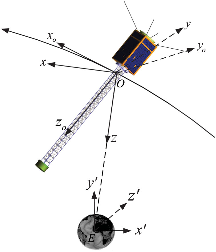
Figure 2. Co-ordinate frames.
According to the momentum theorem, without attitude control, the attitude dynamic equation can be expressed as
 \begin{equation}\frac{{d{{\bf{H}}}}}{{dt}} = {{{\bf{M}}}_G} + {{{\bf{M}}}_F}\label{eqn13}\end{equation}
where  ${\bf{M}}_G$ and
  ${\bf{M}}_F$ are the torques produced by the gravity gradient and the thrust, respectively. In the angular momentum
  ${{\bf{H}}} = {{\bf{I}}} \times {{\bf\omega}}$,
  ${{\bf{I}}}$ is the central inertia tensor and the angular velocity vector
  ${{\bf\omega}} = {\bf{l}} \times \dot{{\bf{l}}}$.
The torque  ${\bf{M}}_G$ is written as
 \begin{equation}{{{\bf{M}}}_G} \approx 3\mu {r^{ - 3}}{{\bf{k}}} \times \left( {{{\bf{I}}} \cdot {{\bf{k}}}} \right) = 3\mu {r^{ - 3}}I\left( {{{\bf{l}}} \times {{\bf{k}}}} \right)\left( {{{\bf{l}}} \cdot {{\bf{k}}}} \right)\label{eqn14}\end{equation}
where r is the geocentric distance,  $\mu = 3.986 \times {10^5}{\rm k}{{\rm m}^3}/{{\rm s}^2}$ is the gravitational constant of the Earth and
  $I = Mm{\left( {M + m} \right)^{ - 1}}{l^2}$.
The torque  ${\bf{M}}_F$ is written as
 \begin{equation}{{\bf{M}}_F} = - lm{\left( {M + m} \right)^{ - 1}}{{\bf{F}}} \times {{\bf{l}}}\label{eqn15}\end{equation}
By performing some cumbersome algebraic work, dynamic equations can be obtained as
 \begin{equation}\ddot \theta = - {f_u}{\tilde l^{ - 1}}\cos \theta {\left( {\cos \phi } \right)^{ - 1}} - 3\mu {r^{ - 3}}\cos \theta \sin \theta - 2\left( {\dot u - \dot \theta } \right)\dot \phi \tan \phi + \ddot u\label{eqn16}\end{equation}
 \begin{equation}\ddot \phi = \left[ {{f_u}{{\tilde l}^{ - 1}}\sin \theta - 3\mu {r^{ - 3}}{{\cos }^2}\theta \cos \phi - {{\left( {\dot u - \dot \theta } \right)}^2}\cos \phi } \right]\sin \phi\label{eqn17}\end{equation}
where  $\tilde l = lM{\left( {M + m} \right)^{ - 1}}$.
In the dynamic model, the equilibrium position of  $\phi \equiv 0$ exists; besides, as the initial value of the roll angle is very small, the coupling of the pitch angle
  $\theta$ and the roll angle
  $\phi$ is not obvious in orbital transfer. Hence, the properties of equilibrium positions of the pitch angle
  $\theta$ can be obtained in Table 1, where
  ${k_u} = {f_u}{r^3}{\left( {3\mu \tilde l} \right)^{ - 1}}$.
Table 1 Properties of equilibrium positions of the pitch angle  $\theta$

In this paper, it is assumed that at any certain moment, the parameter  $k_u$ is constant, and the equilibrium position derived for this condition is defined as the expected attitude angle at this moment.
Definition 1 Considering the time-varying geocentric distance  $r\left( t \right)$ and the thrust acceleration component
  ${f_u}$, at the moment of
  $t = \tau $, the value of
  $r\left( t \right)$ is
  ${\left. r \right|_{t = \tau }}$. In the orbital transfer between two co-planar orbits, the expected pitch angle
  ${\theta _c}\left( t \right)$ and the roll angle
  ${\phi_c} \left(t\right)$ (the expected attitude trajectory) are defined as
 \begin{equation}\begin{array}{l}{\left. {{\theta _c}\left( t \right)} \right|_{t = \tau }} = \left\{ {{{\tilde \theta }_e} \in {\theta _e}:{k_u} = {f_u}{{\left( {{{\left. r \right|}_{t{ = _\tau }}}} \right)}^3}\left( {3\mu {{\tilde l}}} \right)^{-1}} \right\}\\{\left. {{\phi _c}\left( t \right)} \right|_{t = \tau }} \equiv 0\end{array}\label{eqn18}\end{equation}
where  ${{{\tilde \theta }_e}}$ is a stable center of the equilibrium position
  $\theta_e$.
Remark 2 The designed trajectory helps avoid the attitude disorder of the gravity gradient microsatellite. Besides, as the pitch angle  $\theta$ approaches to the expected attitude trajectory, the torque
  ${\bf{M}}_F$ can be compensated by the torque
  ${\bf{M}}_G$; thus, it effectively reduces the energy consumption of the attitude controller.
4.2 Magnetic attitude tracking control
In engineering, the control torque  ${\bf{M}}_C$ generated by the magnetorquer is constrained in the plane, which is perpendicular to the local geomagnetic field vector, so it is impossible to obtain an arbitrary ideal magnetic control torque
  ${{\tilde{{\bf{M}}}}}_C$.
To address the problem, the magnetic dipole moment  ${\bf{U}}$ can be applied as
 \begin{equation}{{\bf{U}}} = -\frac{{{{{\tilde{{\bf{M}}}}}_C} \times {{\bf{B}}}}}{{{{\left\| {{\bf{B}}} \right\|}^2}}}\label{eqn19}\end{equation}
Thereby, the actual magnetic control torque acting on the gravity gradient microsatellite is given as
 \begin{equation}{{{\bf{M}}}_C} = - \frac{{{{{\tilde{{\bf{M}}}}}_C} \times {{\bf{B}}}}}{{{{\left\| {{\bf{B}}} \right\|}^2}}} \times {{\bf{B}}}\label{eqn20}\end{equation}
 ${\bf{M}}_C$ is a component of
  $\tilde {{\bf{M}}}_C$ and is perpendicular to
  ${\bf{B}}$. The geometric relation among
  ${\bf{B}}$,
  ${\bf{U}}$,
  $\tilde {{\bf{M}}}_C$ and
  ${{\bf{M}}}_C$ is illustrated in Fig. 4. The control torque is expressed as
  ${{{\bf{M}}}_C} = {\bf{\Gamma} _B}{{\tilde{{\bf{M}}}}_C}$, where
  ${\bf{\Gamma} _B}$ is a singular matrix.

Figure 4. The geometric relation among  ${\bf{B}}$,
  ${\bf{U}}$,
  $\tilde {{\bf{M}}}_C$ and
  ${{\bf{M}}}_C.$
Remark 3 The control torque generated by the magnetorquer is constrained by the magnetic field, so the controllability of the designed controller cannot be guaranteed in the global field; however, if the value of the angular velocity  ${\bf\omega}$ is small and
  $0 \lt \mathop {\lim }\limits_{T \to \infty } \frac{1}{T}\int_0^T {{\bf{\Gamma} _B}dt} \lt {{{\bf{I}}}_3}$, the attitude of the gravity gradient microsatellite can be controlled(Reference Lovera and Astolfi11).
Obviously, the global stability of the system in existing control methods depends on  ${\bf\omega}$ and
  $\bf{\Gamma}_B$ to a large extent, and the control performance is greatly influenced by the magnetic constraint. In order to solve the problem, an auxiliary compensator is designed in this paper, and a compensator-based sliding mode control is presented.
The basic idea of the auxiliary compensator is to introduce control modifications in order to recover, as much as possible, the performance induced by a previous design carried out on the basis of the unconstrained (without magnetic constraint) system. Thus, the general principle of the control scheme is depicted in Fig. 5. The auxiliary compensator is driven by the difference  $\Delta {\bf{M}}_C$ between the constrained and unconstrained control signals (
 ${\bf{M}}_C$ and
  $\tilde{{\bf{M}}}_C$). The auxiliary compensator itself emits one signal
  $\bf{\lambda}$, which is directly fed into the improved controller. It is not easy to realise the attitude tracking (
 $\bf{\Phi} -\bf{\Phi}_c \to 0$) directly in the presence of the magnetic constraint, but a controller can be designed to make
  $\bf{\Phi} -\bf{\Phi}_c + \bf{\lambda}$ approach zero. Besides, the designed auxiliary compensator can realise
  $\bf{\lambda} \to 0$ if
  $\Delta {\bf{M}}_C$ is bounded. Then, the stability of the system can be ensured.

Figure 5. The principle of closed-loop control.
The adaptive auxiliary compensator is designed as
 \begin{equation}{\dot{\bf{\lambda}}} = {{\bf{A}}\bf{\lambda}} + {{\bf{C}}}\Delta {{{\bf{M}}}_C}\label{eqn21}\end{equation}
where  ${\bf{\lambda}} = {\left[ {{\lambda _1},{\lambda _2},{\lambda _3},{\lambda _4},{\lambda _5},{\lambda _6}} \right]^T}$,
  ${\bf{A}}$ and
  ${\bf{C}}$ are written as
 \begin{equation}{{\bf{A}}} = \left[ {\begin{array}{*{20}{c}}{ - {a_1}}&1&0&0&0&0\\0&{ - {a_2}}&0&0&0&0\\0&0&{ - {a_3}}&1&0&0\\0&0&0&{ - {a_4}}&0&0\\0&0&0&0&{ - {a_5}}&1\\0&0&0&0&0&{ - {a_6}}\end{array}} \right],\;{{\bf{C}}} = \left[ {\begin{array}{*{20}{c}}0&0&0\\{{c_1}}&0&0\\0&0&0\\0&{{c_2}}&0\\0&0&0\\0&0&{{c_3}}\end{array}} \right]\label{eqn22}\end{equation}
Remark 4 To ensure that  ${\lambda _i} \to 0\;\left( {i = 1,2, \cdots ,6} \right)$,
  ${\bf{A}}$ should be Hurwitz; in other words,
  ${a_i} > 0\;\left( {i = 1,2, \cdots ,6} \right)$. Besides, in order to avoid the instability aroused by
  $\Delta {{{\bf{M}}}_C}$ that is too large,
  ${a_i}$ needs to be large enough(Reference Bechlioulis and Rovithakis15).
Lemma 1 (Reference Vadali16) The sliding surface is designed as
 \begin{equation}{{\bf{s}}} = \left( {{{{\bf\omega}}_r} - {{{\bf\omega}}_{rc}}} \right) + {k_q}\left( {{{{\bf{q}}}_r} - {{{\bf{q}}}_{rc}}} \right)\label{eqn23}\end{equation}
where  $\bf{\omega} _{rc}={[0,0,0]^T}$ is the expected angular velocity, and
  ${{{\bf{Q}}}_c} = {\left[ {{{{q}}_{1c}},{{{\bf{q}}}_{rc}}} \right]^T}$ is the expected unit attitude quaternion. If
  ${{\bf{s}}} \equiv {[0,0,0]^T}$, the attitude quaternion
  ${\bf{Q}}$ exponentially converges to
  ${\bf{Q}}_c$.
Based on Lemma 1, the improved sliding surface  $\tilde{{\bf{s}}}$ is designed as
 \begin{equation}{\tilde{{\bf{s}}}} = {{\bf{s}}} + {{{\bf{s}}}_\lambda }\label{eqn24}\end{equation}
where  ${{{\bf{s}}}_\lambda } = {\left[ {{{\dot \lambda }_1},{{\dot \lambda }_3},{{\dot \lambda }_5}} \right]^T} + {k_q}{\left[ {{\lambda _1},{\lambda _3},{\lambda _5}} \right]^T}$.
Theorem 1 Considering the system described by Equation (1) and Definition 1, if a sliding mode controller is designed as
 \begin{equation}{{\tilde{{\bf{M}}}}_C} = -{{\bf{f}}}\left( {{{\bf\omega}},t} \right) - {{\bf{I}}}\bf{\xi}- {\bf{I}}{{\dot{{\bf{s}}}}_\lambda } - {k_s}{\tilde{{\bf{s}}}} - \eta {\mathop{\rm sgn}} \left( {\tilde{{\bf{s}}}} \right)\label{eqn25}\end{equation}
 \begin{equation}{{{\bf{M}}}_C} = - \left( {{{{{{\tilde{{\bf{M}}}}}_C} \times {{\bf{B}}}} \mathord{\left/ {\vphantom {{{{{\tilde{{\bf{M}}}}}_C} \times {{\bf{B}}}} {{{\left\| {{\bf{B}}} \right\|}^2}}}} \right.} {{{\left\| {{\bf{B}}} \right\|}^2}}}} \right) \times {{\bf{B}}}\label{eqn26}\end{equation}
where  $\eta \gt \Delta{f_{\max }}\left( {{\bf{\omega}},t} \right) + \Delta{d_{\max }}\left( t \right)$ and
  ${\bf{\xi}} = - {{{\dot{\bf\omega}}}_o} + \frac{1}{2}{k_q}\left( {{q_1}{{{\bf\omega}}_r} - {{\bf\omega}}_r^ \times {{{\bf{q}}}_r}} \right)$, then attitude angles will track the expected attitude trajectory
  ${{\bf{\Phi}}_c} = {\left[ {{\psi _c}\left( t \right),{\theta _c}\left( t \right),{\phi _c}\left( t \right)} \right]^T}$.
Proof
The Lyapunov function is designed as
 \begin{equation}V = \frac{1}{2}{{\tilde{{\bf{s}}}}^T}{\bf{I}}{\tilde{{\bf{s}}}}\label{eqn27}\end{equation}
Considering the designed controller, the derivative of the Lyapunov function can be obtained as
 \begin{equation}\begin{array}{l}\dot V = {{\tilde{{\bf{s}}}}^T}{\bf{I}}{\dot{\tilde{{\bf{s}}}}} = {{\tilde{{\bf{s}}}}^T}\left( {{\bf{I}}{{\dot{\bf\omega}}} + {\bf{I}}{\bf{\xi}}}+ {\bf{I}}{{\dot{{\bf{s}}}}_\lambda } \right)\\[6pt]\;\;\; = {{\tilde{{\bf{s}}}}^T}\left[ {\Delta {{\bf{f}}}\left( {{{\bf\omega}},t} \right) + \Delta {\bf{d}}\left( t \right) - {k_s}{\tilde{{\bf{s}}}} - \eta {\rm{sgn}}\left( {\tilde{{\bf{s}}}} \right)} \right]\\[6pt]\;\;\; = - {k_s}{{\tilde{{\bf{s}}}}^T}{\tilde{{\bf{s}}}} + {{\tilde{{\bf{s}}}}^T}\left[ {\Delta {{\bf{f}}}\left( {\omega ,t} \right) + \Delta {\bf{d}}\left( t \right)} \right] - \eta {\left\| {\tilde{{\bf{s}}}} \right\|_1}\end{array}\label{eqn28}\end{equation}
As  $\eta > \Delta{f_{\max }}\left( {{\bf{\omega}},t} \right) + \Delta{d_{\max }}\left( t \right)$,
  $\dot V \le 0$. If and only if
  ${\tilde{{\bf{s}}}} = {[0,0,0]^T}$,
  $\dot V=0$.
Remark 5 Initially, the Lyapunov function V is bounded. In light of Equations (27) and (28),  $\Delta {{{\bf{M}}}_C}$ can be bounded when
  $t \to \infty$. By setting
  ${\bf{A}}$,
  ${\lambda _i} \to 0 \;\left( {i = 1,2, \cdots ,6} \right)$ can be realised(Reference Bechlioulis and Rovithakis15); thus, as
  ${{\tilde{{\bf{s}}}} }\to 0$,
  $\bf{\Phi} \to {\bf{\Phi} _c}$.
Remark 6 It should be noted that as the pitch angle  $\theta$ approaches the expected attitude trajectory, the torque
  ${\bf{M}}_F$ can be compensated by the torque
  ${\bf{M}}_G$. At this moment,
  $\tilde {{\bf{M}}}_C$ approaches zero and
  $\Delta {\bf{M}}_C \to 0$.
5.0 CASE STUDY
In engineering, the gravity gradient microsatellite is mainly utilised to explore the space environment in a LEO. The orbit altitude is within the range of 400–800km. In order to obtain global spatial data, it is requested to increase the orbit altitude by at least 0.1–1km in orbital transfer. The electric thrust imposed on the main-sat is within the range of  $0.1$–100mN; accordingly, the torque produced by the thrust varies within the range of
  $10^{-5}$–
 $10^{-2}$N
  $\cdot$ m. The torque produced by the gravity approaches to
  $10^{-5}$N
  $\cdot$ m. The external torques (the atmosphere drag torque and the solar pressure torque) are within the range of
  $10^{-7}$–
 $10^{-6}$N
  $\cdot$ m.
Without loss of generality, the geocentric distance of the initial circular orbit is 7000km. The thrust F is  $0.1$mN and always along the transversal direction of the mass center. The masses of the main-sat and the sub-sat are 30 and 5kg, respectively. The length of the coilable mast is 2m. Based on the dumbbell model, the momentum of inertia
  $I=17.14$kg
  $\cdot$ m
 $^2$; meanwhile, the inertial matrix
  ${\bf{I}} \approx diag\{ 18.141,\;18.141,\;0.458\}$
  $\textrm{kg} \cdot {m^2}$ in the rigid body model. Initially, attitude angles
  $\psi$,
  $\theta$ and
  $\phi$ are
  $1^\circ$,
  $1^\circ$ and
  $1^\circ$, respectively. Controller parameters are selected as
  ${k_q} = 1.25 \times {10^{ - 3}}$,
  ${k_s} = 7.5 \times {10^{ - 2}}$,
  $\eta = 1 \times {10^{ - 6}}$,
  ${a_i} = 1\;\left( {i = 1,2, \cdots ,6} \right)$ and
  ${c_j} = 1\;\left( {j = 1,2,3} \right)$.
As shown in Fig. 6, when the thrust imposed on the gravity gradient microsatellite is along the transversal direction, the geocentric distance will be increased by 31m per orbit period. If the controller is not adopted,  $\psi$ and
  $\phi$ will dramatically change within the range of
  $-60^\circ\sim 180^\circ$ and
  $-180^\circ \sim 60^\circ$ in the first ten orbit periods, respectively; meanwhile,
  $\theta$ maintains the periodical motion within a large range of
  $-90^\circ \sim 0^\circ$, which goes against the flight safety of the gravity gradient microsatellite. In order to inhibit the serious pendular motion, the designed magnetic attitude tracking control is implemented in orbital transfer.
  $\psi$ and
  $\phi$ vary in a small range and approach
  $0^\circ$; in the meantime,
  $\theta$ gradually converges to the expected attitude trajectory.
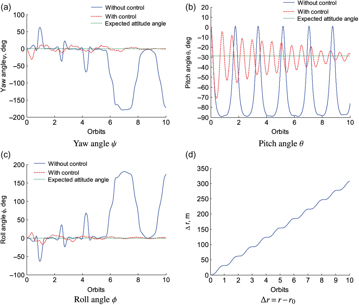
Figure 6. The comparison between the controlled and uncontrolled systems.
Remark 7 According to Definition 1, the expected pitch angle  $\theta_c$ is time varying, because the geocentric distance r is increased in orbital transfer. Initially,
  $\theta_c \approx -28.5589^\circ$. In the 10th orbit period,
  $\theta_c$ approaches
  $-28.5629^\circ$. The change of
  $\theta_c$ is not obvious in the figure, which is conducive for the flight safety.
To demonstrate the improvement in performance from the auxiliary compensator, both cases, with and without the compensator, are studied in Fig. 7. In the case without the compensator, the auxiliary compensator is not adopted, and  ${\bf{s}}_\lambda$ is not considered in Theorem 1. Meanwhile, other control parameters remain unchanged. Obviously, with respect to the case with the compensator, attitude angles vary within a larger range; in addition, in the last four orbit periods, the attitude tracking speed is slow, and the control performance is not good.
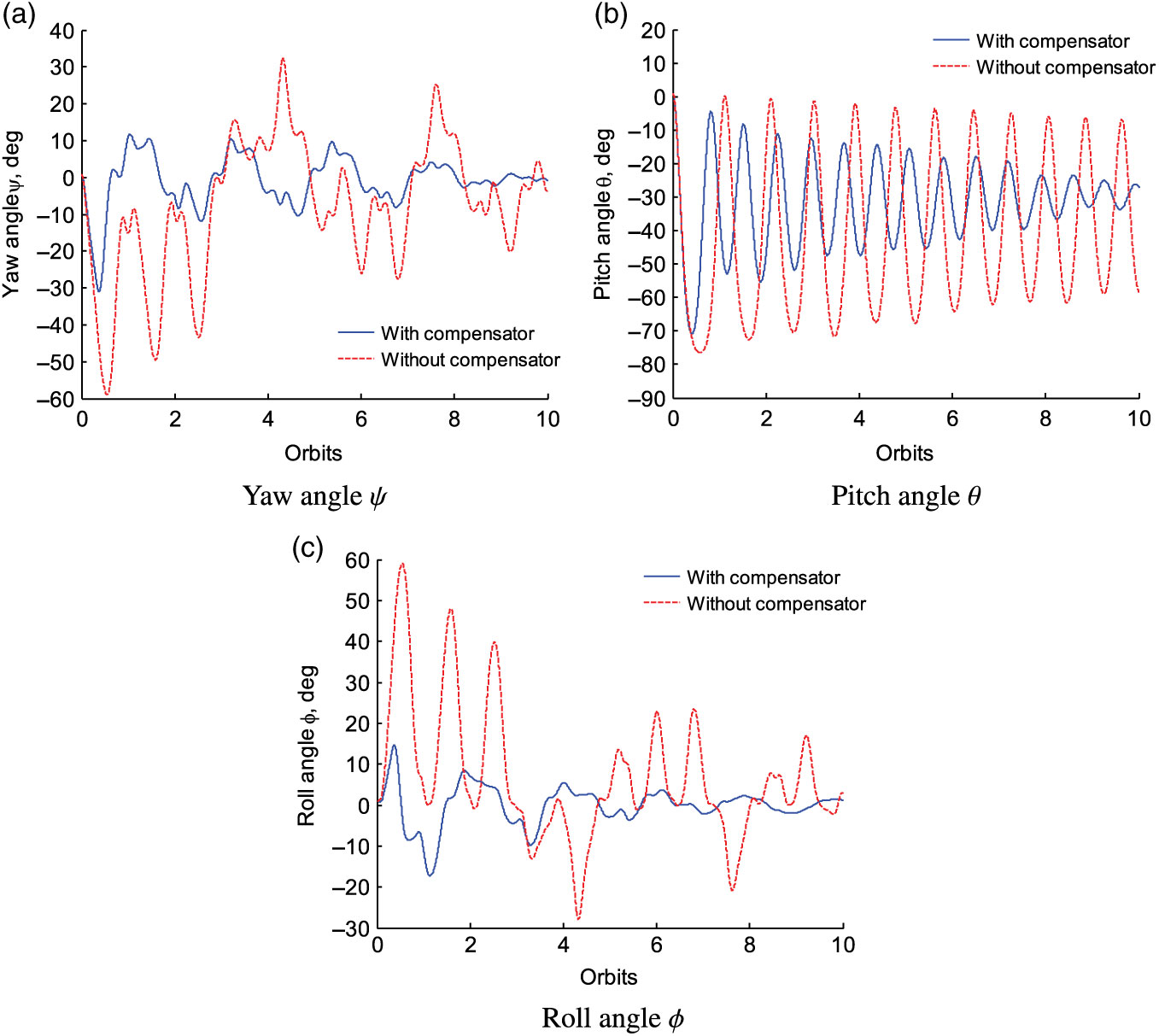
Figure 7. Control results with and without compensator.
As shown in Fig. 8, with the compensator,  $M_C$ and
  $\Delta M_C$ gradually tend to 0N
  $\cdot$ m. After the 8th orbit period, torque components
  ${M_{Fx}} \approx 0$N
  $\cdot$ m,
  ${M_{Fz}} \approx 0$N
  $\cdot$ m,
  ${M_{Gx}} \approx 0$N
  $\cdot$ m and
  ${M_{Gz}} \approx 0$N
  $\cdot$ m; meanwhile,
  ${M_{Fy}}$ and
  ${M_{Gy}}$ approach
  $-2.51 \times {10^{ - 5}}$N
  $\cdot$ m and
  $2.58 \times {10^{ - 5}}$N
  $\cdot$ m, respectively. It is clear that the torque
  ${\bf{M}}_F$ can be compensated by the torque
  ${\bf{M}}_G$, and the error
  $0.07\times {10^{ - 5}}$N
  $\cdot$ m is caused by the the momentum of inertia difference between the dumbbell model and the rigid body model.
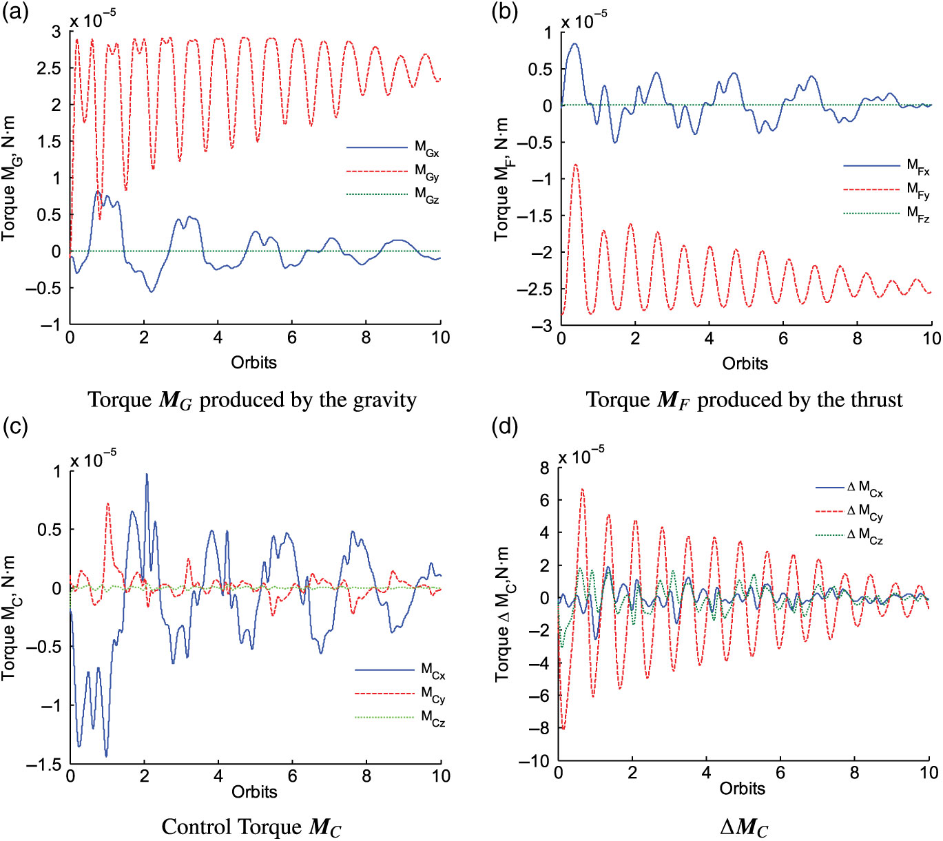
Figure 8. The time responses of torques  ${\bf{M}}_G$,
  ${\bf{M}}_F$,
  ${\bf{M}}_C$ and
  $\Delta {\bf{M}}_C.$
6.0 CONCLUSIONS
Based on a series of analyses and simulations, the following conclusions can be drawn:
(1) If a transversal electric thrust is applied to the gravity gradient microsatellite in an orbital transfer, the equilibrium position of the pitch angle  $\theta$ exists; besides, the number and stability of the equilibrium position are closely related to r, M, m, l and F;
(2) As the pitch angle approaches the proposed expected attitude trajectory, the torque  ${\bf{M}}_F$ can be compensated by the torque
  ${\bf{M}}_G$, which can help reduce the energy consumption and avoid the attitude disorder;
(3) The method of the magnetic control presented in this paper can address the attitude tracking control problem subject to the magnetic constraint. The proposed sliding mode control based on the auxiliary compensator is conducive for enhancing the robustness and stability of the system.
In general, the proposed magnetic attitude tracking control scheme is beneficial for avoiding the attitude disorder and to reduce the energy consumption of the magnetorquer, which can provide a reference for research on the gravity gradient microsatellite in orbital transfer.
ACKNOWLEDGEMENTS
This research was funded by the National Natural Science Foundation of China under Grant No. 11602008 and Grant No. 11572016.


