2. Model and Problem Formulation

Suppose that an insurance company has two dependent classes of insurance business such as motor and life insurance. Let {X _i , i≥1} be the claim size random variables for the first class following a common distribution F _X (x) with F _X (x)=0 for x≤0, and 0<F _X (x)≤1 for x>0; and {Y _i , i≥1} be the claim size random variables for the second class following a common distribution F _Y (y) with F _Y (y)=0 for y≤0, 0<F _Y (y)≤1 for y>0. Then, the aggregate claims process generated from these two classes of business is given by

$$S_{t} {\equals}S_{1} (t){\plus}S_{2} (t){\equals}\mathop \sum\limits_{i{\equals}1}^{N_{1} (t){\plus}N(t)} X_{i} {\plus}\mathop \sum\limits_{i{\equals}1}^{N_{2} (t){\plus}N(t)} Y_{i} $$

where N _i (t)+N(t) (i=1, 2) is the claim number process for class i (i=1, 2), and N ₁(t), N ₂(t) and N(t) are three independent Poisson processes with parameters λ ₁, λ ₂ and λ, respectively. Assume that X _i and Y _i are independent claim size random variables, and that they are independent of N ₁(t), N ₂(t) and N(t). It is obvious that the dependence of the two classes of business is due to a common shock governed by the counting process N(t).

We allow the insurance company to continuously reinsure a fraction of its claim with the retention levels q ₁(⋅)∈[0,1] and q ₂(⋅)∈[0,1] for X _i and Y _i , respectively, and the reinsurance premium rate at time t is δ(q ₁(⋅), q ₂(⋅)). Let {U _t , t≥0} denote the associated surplus process, i.e., U _t is the surplus of the insurer at time t under the strategy (q ₁(U _t ), q ₂(U _t )). This controlled surplus process can be given by

(2.1) $$dU_{t} {\equals}\left( {c{\minus}\delta (q_{1} \left( {U_{t} } \right),q_{2} \left( {U_{t} } \right)} \right)dt{\minus}q_{1} \left( {U_{t} } \right)dS_{1} \left( t \right){\minus}q_{2} \left( {U_{t} } \right)dS_{2} \left( t \right)$$

where the constant c is the premium rate. Moreover, from Grandell (Reference Grandell1991), we know that the Brownian motion risk model given by

$$\hat{S}_{1} \left( t \right){\equals}a_{1} {}^{t} {\minus}b_{1} B_{{1t}} $$

with a ₁=(λ ₁+λ)E(X) and $b_{1}^{2} {\equals}\left( {\lambda _{1} {\plus}\lambda } \right)E\left( {X^{2} } \right)$ can be seen as a diffusion approximation to the compound Poisson process S ₁(t). Similarly,

$$\hat{S}_{2} (t){\equals}a_{2} t{\minus}b_{2} B_{{2t}} $$

with a ₂=(λ ₂ + λ)E(Y) and $b_{2}^{2} {\equals}\left( {\lambda _{2} {\plus}\lambda } \right)E\left( {Y^{2} } \right)$ can be treated as a diffusion approximation to the compound Poisson process S ₂(t). Here, B _1t and B _2t are standard Brownian motions with the correlation coefficient

$$\rho {\equals}{{\lambda E\left( X \right)E\left( Y \right)} \over {\sqrt {\left( {\lambda _{1} {\plus}\lambda } \right)E\left( {X^{2} } \right)\left( {\lambda _{2} {\plus}\lambda } \right)E\left( {Y^{2} } \right)} }}$$

Thus, E[B _1t B _2t ]=ρt. With expected value principle:

$$c{\equals}\left( {1{\plus}\theta _{1} } \right)a_{1} {\plus}\left( {1{\plus}\theta _{2} } \right)a_{2} $$

and the reinsurance premium rate at time t is

$$\delta \left( {q_{1} \left( {U_{t} } \right),q_{2} \left( {U_{t} } \right)} \right){\equals}\left( {1{\plus}\eta _{1} } \right)\left( {1{\minus}q_{1} \left( {U_{t} } \right)} \right)a_{1} {\plus}\left( {1{\plus}\eta _{2} } \right)\left( {1{\minus}q_{2} \left( {U_{t} } \right)} \right)a_{2} $$

where θ _i (i=1, 2) and η _i (i=1, 2) are the insurer’s and reinsurer’s safety loading of the two classes of the insurance business, respectively. Without loss of generality, we assume that η _i ≥θ _i , and η _i >θ _i holds at least for one i (i=1,2), otherwise the problem becomes trivial.

Replace S _i (t)(i=1, 2) by $\hat{S}_{i} (t){\rm }(i{\equals}1,2)$ in (2.1). Furthermore, we assume that the insurer is allowed to invest all its surplus in a risk-free asset (bond or bank account) with interest rate r. Then the process evolves as

$$\eqalignno{ d\hat{U}_{t} {\equals} &#x0026; \left[ {r\hat{U}_{t} {\plus}a_{1} \left( {\theta _{1} {\minus}\eta _{1} {\plus}\eta _{1} q_{1} \left( {\hat{U}_{t} } \right)} \right)} \right.\left. {{\plus}a_{2} \left( {\theta _{2} {\minus}\eta _{2} {\plus}\eta _{2} q_{2} \left( {\hat{U}_{t} } \right)} \right)} \right]dt \cr &#x0026; {\rm }{\plus} b_{1} q_{1} \left( {\hat{U}_{t} } \right)dB_{{1t}} {\plus}b_{2} q_{2} \left( {\hat{U}_{t} } \right)dB_{{2t}} $$

or equivalently:

(2.2) $$\eqalignno{ d\hat{U}_{t} {\equals} &#x0026; \left[ {r\hat{U}_{t} {\plus}a_{1} \left( {\theta _{1} {\minus}\eta _{1} {\plus}\eta _{1} q_{1} \left( {\hat{U}_{t} } \right)} \right){\plus}a_{2} \left( {\theta _{2} {\minus}\eta _{2} {\plus}\eta _{2} q_{2} \left( {\hat{U}_{t} } \right)} \right)} \right]dt \cr &#x0026; {\rm }{\plus} \sqrt {b_{1}^{2} q_{1}^{2} \left( {\hat{U}_{t} } \right){\plus}b_{2}^{2} q_{2}^{2} \left( {\hat{U}_{t} } \right){\plus}2b_{1} b_{2} q_{1} \left( {\hat{U}_{t} } \right)q_{2} \left( {\hat{U}_{t} } \right)\rho } dB_{t} $$

with $\hat{U}_{0} {\equals}u$ and $B_{t} $ is a standard Brownian motion. The similar model has also been studied in the literature; see, for example, Yuen et al. (Reference Yuen, Liang and Zhou2015), Liang & Yuen (Reference Liang and Yuen2016), Bi et al. (Reference Bi, Liang and Xu2016) and the references therein.

Define the maximum surplus value M _t at time t by

$$M_{t} {\equals}{\rm max}\left\{ {\mathop{{{\rm sup}}}\limits_{{0\leq s\leq t}} \hat{U}_{s} ,M_{0} } \right\}$$

where M ₀=m>0. Note that we allow the surplus process to have a financial past, and that m is no less than the initial surplus u by definition. We mean that when the value of the surplus process reaches α∈[0,1) times its maximum value, then drawdown occurs. Define the corresponding hitting time by

$$\tau _{\alpha } \,\colon\,\,{\equals}{\rm inf}\left\{ {t\geq 0\,\colon\,\hat{U}_{t} \leq \alpha M_{t} } \right\}$$

We can see that, if α=0, then we are in the case of minimising the probability of ruin for the fixed ruin level 0. Besides, if the value of the investment fund is big enough, say, at least

$${{a_{1} \left( {\eta _{1} {\minus}\theta _{1} } \right){\plus}a_{2} \left( {\eta _{2} {\minus}\theta _{2} } \right)} \over r}$$

then the insurer can transfer all the risk, and the surplus value will never decrease, i.e., drawdown cannot occur in this case. We generalise from this case in the following Remark 2.1.

$$u_{s} {\equals}{{a_{1} \left( {\eta _{1} {\minus}\theta _{1} } \right){\plus}a_{2} \left( {\eta _{2} {\minus}\theta _{2} } \right)} \over r}$$

such that

$$a_{1} \left( {\theta _{1} {\minus}\eta _{1} } \right){\plus}a_{2} \left( {\theta _{2} {\minus}\eta _{2} } \right){\plus}ru\,\gt\,0,{\rm for}\,{\rm all}\,u\,\gt\,u_{s} $$

and

$$a_{1} \left( {\theta _{1} {\minus}\eta _{1} } \right){\plus}a_{2} \left( {\theta _{2} {\minus}\eta _{2} } \right){\plus}ru\,\lt\,0,{\rm for}\,{\rm all}\,u\,\lt\,u_{s} $$

If $\hat{U}_{0} {\equals}u\geq u_{s} $ , then we can set $q_{1}^{{\rm {\asterisk}}} (\hat{U}_{t} ){\equals}0$ , $q_{2}^{{\rm {\asterisk}}} (\hat{U}_{t} ){\equals}0$ for all t≥0, which implies

$$d\hat{U}_{t} {\equals}\left[ {r\hat{U}_{t} {\plus}a_{1} (\theta _{1} {\minus}\eta _{1} ){\plus}a_{2} (\theta _{2} {\minus}\eta _{2} )} \right]dt\geq 0$$

Under this reinsurance strategy, the value of the surplus process is non-decreasing, so drawdown will never occur. For this reason, we call u _s safe level as defined in Angoshtari et al. (Reference Angoshtari, Bayraktar and Young2016a ).

In the following definition, we give the admissible set of $$\left( {q_{1} \left( {\hat{U}_{t} } \right),q_{2} \left( {\hat{U}_{t} } \right)} \right)$$ .

The set of all admissible strategies is denoted by ${\cal D}$ .

Now assume that the insurer is interested in minimising the probability of drawdown, we denote the minimum probability of drawdown by ϕ(u, m), which depends on the initial surplus u and the maximum (past) value m. Specifically, ϕ is the minimum probability of τ _α <∞, thus, we derive the objective function

$$J^{{q_{1} ,q_{2} }} \left( {u,m} \right){\equals}{\bf{P}} ^{{u,m}} \left( {\tau _{\alpha } \,\lt\,\infty} \right){\equals}{\bf E}^{{u,m}} \left( {{\bf 1}_{{\left\{ {\tau _{\alpha } \,\lt\,\infty} \right\}}} } \right)$$

Here, P ^u,m and E ^u,m denote the probability and expectation, respectively, conditional on $\hat{U}_{0} {\equals}u$ and $M_{0} {\equals}m$ . Then, the corresponding value function is given by

$$\phi (u,m){\equals}\mathop{{{\rm inf}}}\limits_{{q_{1} ,q_{2} \in{\cal D}}} J^{{q_{1} ,q_{2} }} (u,m)$$

3. Minimising the Probability of Drawdown When m≥u _s

We first consider the case for which m≥u _s . Note that if αm>u _s , then the probability of drawdown ϕ(u,m)=1 for all u≤αm, and when u≤αm, we have u>u _s , then according to Remark 2.1, the value of the surplus will consistently increase, and thus the probability of drawdown ϕ(u,m)=0 for all u >αm. In the following context, we shall investigate the case of αm≤u _s in detail. When $\hat{U}_{0} {\equals}u\geq u_{s} $ , the drawdown is impossible; and when $\hat{U}_{0} {\equals}u\leq \alpha m$ , then the drawdown has occurred and the game is over. Therefore, we assume that $\hat{U}_{0} {\equals}u\in[\alpha m,u_{s} ]$ . $\hat{U}_{0} {\equals}u\leq u_{s} $ implies that either $\hat{U}_{t} \,\lt\,u_{s} $ almost surely, for all t≥0, or $\hat{U}_{t} {\equals}u_{s} $ for some t>0. Since $m\geq u_{s} $ , M _t =m holds almost surely for all t≥0. Therefore, avoiding drawdown is equivalent to avoiding ruin with a (fixed) ruin level of αm.

From Bäuerle & Bayraktar (Reference Bäuerle and Bayraktar2014), we can see that the optimal proportional reinsurance strategy with no constraint is the one that maximises the ratio of the drift of the surplus process to its volatility squared in (2.2). Thus, when the arguments u and m indicate the initial surplus and the maximum (past) value, respectively, the Proposition 3.1 can be derived.

(3.1) $$ \scale98% { \left\{ \matrix{ \hat{q}_{1} (u){\equals}{{2\left[ {{\rm \Delta }_{1} {\plus}ru} \right]\left( {a_{2} \eta _{2} \rho b_{1} b_{2} {\minus}a_{1} \eta _{1} b_{2}^{2} } \right)} \over {{\rm \Delta }_{2} }} \hfill \cr \hat{q}_{2} (u){\equals}{{2\left[ {{\rm \Delta }_{1} {\plus}ru} \right]\left( {a_{1} \eta _{1} \rho b_{1} b_{2} {\minus}a_{2} \eta _{2} b_{1}^{2} } \right)} \over {{\rm \Delta }_{2} }} \hfill \cr} \right.$$

in which Δ₁ and Δ₂ are defined by

(3.2) $$\left\{ \matrix{ {\rm \Delta }_{1} {\equals}a_{1} \left( {\theta _{1} {\minus}\eta _{1} } \right){\plus}a_{2} \left( {\theta _{2} {\minus}\eta _{2} } \right)\,\lt\,0 \hfill \cr {\rm \Delta }_{2} {\equals}b_{1}^{2} a_{2}^{2} \eta _{2}^{2} {\plus}b_{2}^{2} a_{1}^{2} \eta _{1}^{2} {\minus}2b_{1} b_{2} a_{1} a_{2} \eta _{1} \eta _{2} \rho \,\gt\,0 \hfill \cr} \right.$$

(3.3) $$\xi (u){\equals}{{\mu \left( {u,q_{1} ,q_{2} } \right)} \over {\sigma ^{2} \left( {u,q_{1} ,q_{2} } \right)}}{\equals}{{a_{1} \left( {\theta _{1} {\minus}\eta _{1} {\plus}\eta _{1} q_{1} \left( u \right)} \right){\plus}a_{2} \left( {\theta _{2} {\minus}\eta _{2} {\plus}\eta _{2} q_{2} \left( u \right)} \right){\plus}ru} \over {b_{1}^{2} q_{1}^{2} \left( u \right){\plus}b_{2}^{2} q_{2}^{2} \left( u \right){\plus}2b_{1} b_{2} q_{1} \left( u \right)q_{2} \left( u \right)\rho }}$$

Differentiating ξ(u) with respect to q ₁(u) and q ₂(u), respectively, we have

$$ \scale98% { \left\{ \matrix{ a_{1} \eta _{1} \left( {b_{1}^{2} \hat{q}_{1}^{2} \left( u \right){\plus}b_{2}^{2} \hat{q}_{2}^{2} \left( u \right){\plus}2b_{1} b_{2} \hat{q}_{1} \left( u \right)\hat{q}_{2} \left( u \right)\rho } \right) \hfill \cr {\minus}\left[ {a_{1} \left( {\theta _{1} {\minus}\eta _{1} {\plus}\eta _{1} \hat{q}_{1} \left( u \right)} \right){\plus}a_{2} \left( {\theta _{2} {\minus}\eta _{2} {\plus}\eta _{2} \hat{q}_{2} \left( u \right)} \right){\plus}ru} \right]\left( {2\hat{q}_{1} \left( u \right)b_{1}^{2} {\plus}2\hat{q}_{2} \left( u \right)b_{1} b_{2} \rho } \right){\equals}0 \hfill \cr a_{2} \eta _{2} \left( {b_{1}^{2} \hat{q}_{1}^{2} \left( u \right){\plus}b_{2}^{2} \hat{q}_{2}^{2} \left( u \right){\plus}2b_{1} b_{2} \hat{q}_{1} \left( u \right)\hat{q}_{2} \left( u \right)\rho } \right) \hfill \cr {\minus}\left[ {a_{1} \left( {\theta _{1} {\minus}\eta _{1} {\plus}\eta _{1} \hat{q}_{1} \left( u \right)} \right){\plus}a_{2} \left( {\theta _{2} {\minus}\eta _{2} {\plus}\eta _{2} \hat{q}_{2} \left( u \right)} \right){\plus}ru} \right]\left( {2\hat{q}_{2} \left( u \right)b_{2}^{2} {\plus}2\hat{q}_{1} \left( u \right)b_{1} b_{2} \rho } \right){\equals}0 \hfill \cr} \right.$$

Solving these equations yields the solution (3.1).

On the other hand, by the technique of stochastic control theory and the corresponding HJB equation, we can also get the candidate optimiser (see e.g., (4.3)) along the same lines in section 4, which is exactly the same as the one in (3.1). Therefore, we can directly come to the conclusion that the solution given by (3.1) is indeed the optimal proportional reinsurance strategy for the case with no constraint.□

From Bäuerle & Bayraktar (Reference Bäuerle and Bayraktar2014, theorem 4.1) and Karatzas & Shreve(Reference Karatzas and Shreve1991: 339), we have the following lemma.

$$\phi (u,m){\equals}1{\minus}{{g(u,m)} \over {g(u_{s} ,m)}}$$

where g is defined by

(3.4) $$g(u,m){\equals}{\int}_{\alpha m}^u {{\rm exp}} \left\{ {{\minus}2{\int}_{\alpha m}^y {\xi \left( w \right)dw} {\rm \ztbnd }} \right\}dy.$$

Note that g in (3.4) is the scale function associated with the diffusion process in (2.2).

Next, we shall focus on discussing the optimal reinsurance strategy which minimises the probability of drawdown when m≥u _s .

Because of the constraints of $\left( {q_{1}^{{\rm {\asterisk}}} \left( u \right),q_{2}^{{\rm {\asterisk}}} \left( u \right)} \right)$ and the result of $${{{{a_{2} b_{1} } \over {a_{1} \rho b_{2} }}\eta _{2} } \mathord{\left/ {\vphantom {{{{a_{2} b_{1} } \over {a_{1} \rho b_{2} }}\eta _{2} } {{{a_{2} \rho b_{1} } \over {a_{1} b_{2} }}\eta _{2} {\equals}{1 \over {\rho ^{2} }}\,\gt\,1}}} \right. \kern-\nulldelimiterspace} {{{a_{2} \rho b_{1} } \over {a_{1} b_{2} }}\eta _{2} {\equals}{1 \over {\rho ^{2} }}\,\gt\,1}}$$ , to get the optimal strategy and the minimum probability of drawdown, we need to discuss the following three cases:

$$\left\{ {\matrix{ {{\rm Case}\quad 1\,\colon\,\quad {{a_{2} \rho b_{1} } \over {a_{1} b_{2} }}\eta _{2} \,\lt\,\eta _{1} \,\lt\,{{a_{2} b_{1} } \over {a_{1} \rho b_{2} }}\eta _{2} } &#x0026; {\left( {{\rm i}{\rm .e}{\rm .,}\hat{q}_{1} \left( u \right)\,\gt\,0,\hat{q}_{2} \left( u \right)\,\gt\,0} \right)} \cr \hskip-38pt {{\rm Case}\quad 2\,\colon\,\quad \eta _{1} \leq {{a_{2} \rho b_{1} } \over {a_{1} b_{2} }}\eta _{2} } &#x0026; {\left( {{\rm i}{\rm .e}{\rm .,}\hat{q}_{1} \left( u \right)\leq 0,\hat{q}_{2} \left( u \right)\,\gt\,0} \right)} \cr \hskip-38pt {{\rm Case}\quad 3\,\colon\,\quad \eta _{1} \geq {{a_{2} b_{1} } \over {a_{1} \rho b_{2} }}\eta _{2} } &#x0026; {\left( {{\rm i}{\rm .e}{\rm .,}\hat{q}_{1} \left( u \right)\,\gt\,0,\hat{q}_{2} \left( u \right)\leq 0} \right)} \cr } } \right.$$

Since the proof of Case 3 is similar to Case 2, in the following context, we just need to present the proof of Case 1 and Case 2 in detail.

Case 1: ${{a_{2} \rho b_{1} } \over {a_{1} b_{2} }}\eta _{2} \,\lt\,\eta _{1} \,\lt\,{{a_{2} b_{1} } \over {a_{1} \rho b_{2} }}\eta _{2} $ .

In this case, $\hat{q}_{1} (u)\,\gt\,0$ and $\hat{q}_{2} (u)\,\gt\,0$ . Let

$$\left\{ \matrix{ u_{1} {\equals}{1 \over r}\left[ {{{{\rm \Delta }_{2} } \over {2\left( {a_{2} {\rm \eta }_{2} \rho b_{1} b_{2} {\minus}a_{1} \eta _{1} b_{2}^{2} } \right)}}{\minus}{\rm \Delta }_{1} } \right] \hfill \cr u_{2} {\equals}{1 \over r}\left[ {{{{\rm \Delta }_{2} } \over {2\left( {a_{1} \eta _{1} \rho b_{1} b_{2} {\minus}a_{2} \eta _{2} b_{1}^{2} } \right)}}{\minus}{\rm \Delta }_{1} } \right] \hfill \cr} \right.$$

It’s easy to see that $\hat{q}_{1} (u_{1} ){\equals}1$ , $\hat{q}_{2} (u_{2} ){\equals}1$ .

For convenience, we assume that u ₁<u ₂ as similar results can be obtained for u ₁>u ₂. From (3.1), we can see that $\hat{q}_{1} (u)$ , $\hat{q}_{2} (u)$ are decreasing functions w.r.t. u. Thus, when u ₂≤u≤u _s , we have $0\leq \hat{q}_{1} (u)\,\lt\,1$ , $0\leq \hat{q}_{2} (u)\leq 1$ , and hence $q_{1}^{{\rm {\asterisk}}} (u){\equals}\hat{q}_{1} (u)$ , $q_{2}^{{\rm {\asterisk}}} (u){\equals}\hat{q}_{2} (u)$ . One can show that, under this optimal reinsurance strategy given in (3.1), we have

(3.5) $$\xi _{{11}} (u){\equals}{{\mu \left( {u,q_{1}^{{\rm {\asterisk}}} ,q_{2}^{{\rm {\asterisk}}} } \right)} \over {\sigma ^{2} \left( {u,{\it q}_{1}^{{\rm {\asterisk}}} ,q_{2}^{{\rm {\asterisk}}} } \right)}}{\equals}{{{\rm \Delta }_{2} } \over {4\left( {{\minus}{\rm \Delta }_{1} {\minus}ru} \right)b_{1}^{2} \, b_{2}^{2} \left( {1{\minus}\rho ^{2} } \right)}}$$

On the other hand, when $u\leq u_{2} $ , we obtain $\hat{q}_{2} (u)\geq 1$ . Then we have to choose $q_{2}^{{\rm {\asterisk}}} (u){\equals}1$ . Inserting $q_{2}^{{\rm {\asterisk}}} (u){\equals}1$ into (3.3) and maximising the ratio of the drift of the surplus process to its volatility squared, we can get

(3.6) $$\tilde{q}_{1} (u){\equals}{{{\minus}\left( {{\rm \Delta }_{1} {\plus}a_{2} \eta _{2} {\plus}ru} \right){\plus}\sqrt {\left( {B{\plus}ru} \right)^{2} {\minus}4AC} } \over {a_{1} \eta _{1} }}$$

in which A, B, C are defined by

(3.7) $$\left\{ \matrix{ A{\equals}{\minus}{{a_{1}^{2} \eta _{1}^{2} } \over {2b_{1}^{2} }} \hfill \cr B{\equals}a_{1} \left( {\theta _{1} {\minus}\eta _{1} {\minus}{{\rho b_{2} \eta _{1} } \over {b_{1} }}} \right){\plus}a_{2} \theta _{2} \hfill \cr C{\equals}{1 \over 2}b_{2}^{2} \left( {1{\minus}\rho ^{2} } \right) \hfill \cr} \right.$$

From (3.6), we know that $\tilde{q}_{1} (u)$ is also a decreasing function w.r.t. u and when

$$\tilde{u}_{1} {\equals}{1 \over r}\left[ {{{a_{1} \eta _{1} \left( {b_{2}^{2} {\minus}b_{1}^{2} } \right)} \over {2\left( {b_{1}^{2} {\plus}b_{1} b_{2} \rho } \right)}}{\minus}\left( {{\rm \Delta }_{1} {\plus}a_{2} \eta _{2} } \right)} \right]$$

we have $\tilde{q}_{1} (\tilde{u}_{1} ){\equals}1$ . Before we continue our analysis on the optimal results with constraint, we present the following Lemma first.

Proof. Note that

$$\eqalignno{ u_{2} {\minus}\tilde{u}_{1} {\equals} &#x0026; {1 \over r}\left[ {{{{\rm \Delta }_{2} } \over {2\left( {a_{1} \eta _{1} \rho b_{1} b_{2} {\minus}a_{2} \eta _{2} b_{1}^{2} } \right)}}{\minus}{\rm \Delta }_{1} } \right]{\minus}{1 \over r}\left[ {{{a_{1} \eta _{1} \left( {b_{2}^{2} {\minus}b_{1}^{2} } \right)} \over {2\left( {b_{1}^{2} {\plus}b_{1} b_{2} \rho } \right)}}{\minus}\left( {{\rm \Delta }_{1} {\plus}a_{2} \eta _{2} } \right)} \right] \cr {\equals} &#x0026; {{b_{1}^{4} a_{2}^{2} \eta _{2}^{2} {\plus}b_{1}^{3} b_{2} \rho a_{2}^{2} \eta _{2}^{2} {\plus}a_{1} a_{2} \eta _{1} \eta _{2} b_{1}^{4} {\minus}b_{1}^{2} b_{2}^{2} a_{1}^{2} \eta _{1}^{2} {\minus}a_{1}^{2} \eta _{1}^{2} b_{1}^{3} b_{2} \rho {\minus}a_{1} a_{2} \eta _{1} \eta _{2} b_{1}^{2} b_{2}^{2} } \over {2r\left( {b_{1}^{2} {\plus}b_{1} b_{2} \rho } \right)\left( {a_{2} \eta _{2} b_{1}^{2} {\minus}a_{1} \eta _{1} \rho b_{1} b_{2} } \right)}} $$

Because of the assumption of u ₁<u ₂, we have

$$a_{2} \eta _{2} b_{1}^{2} {\minus}a_{1} \eta _{1} \rho b_{1} b_{2} \,\gt\,a_{1} \eta _{1} b_{2}^{2} {\minus}a_{2} \eta _{2} \rho b_{1} b_{2} $$

then,

$$ \eqalignno{ &#x0026; {\rm }b_{1}^{4} a_{2}^{2} \eta _{2}^{2} {\plus}b_{1}^{3} b_{2} \rho a_{2}^{2} \eta _{2}^{2} {\plus}a_{1} a_{2} \eta _{1} \eta _{2} b_{1}^{4} {\minus}b_{1}^{2} b_{2}^{2} a_{1}^{2} \eta _{1}^{2} {\minus}a_{1}^{2} \eta _{1}^{2} b_{1}^{3} b_{2} \rho {\minus}a_{1} a_{2} \eta _{1} \eta _{2} b_{1}^{2} b_{2}^{2} \cr &#x0026; \,\gt\,b_{1}^{2} \left( {a_{1} \eta _{1} b_{2}^{2} {\plus}a_{1} \eta _{1} \rho b_{1} b_{2} } \right){\plus}a_{1} a_{2} \eta _{1} \eta _{2} b_{1}^{4} {\minus}b_{1}^{2} b_{2}^{2} a_{1}^{2} \eta _{1}^{2} {\minus}a_{1}^{2} \eta _{1}^{2} b_{1}^{3} b_{2} \rho {\minus}a_{1} a_{2} \eta _{1} \eta _{2} b_{1}^{2} b_{2}^{2} \cr &#x0026; {\equals}a_{1} a_{2} \eta _{1} \eta _{2} b_{1}^{4} {\minus}b_{1}^{2} b_{2}^{2} a_{1}^{2} \eta _{1}^{2} {\plus}a_{1} \eta _{1} a_{2} \eta _{2} b_{1}^{3} b_{2} \rho {\minus}a_{1}^{2} \eta _{1}^{2} b_{1}^{3} b_{2} \rho \cr &#x0026; \,\gt\,a_{1} \eta _{1} b_{1}^{2} \left( {a_{1} \eta _{1} \rho b_{1} b_{2} {\minus}a_{2} \eta _{2} \rho b_{1} b_{2} } \right){\minus}a_{1} \eta _{1} b_{1}^{2} \left( {a_{1} \eta _{1} \rho b_{1} b_{2} {\minus}a_{2} \eta _{2} \rho b_{1} b_{2} } \right) {\equals}0 $$

In Case 1, it’s clear that

$$2r\left( {b_{1}^{2} {\plus}b_{1} b_{2} \rho } \right)\left( {a_{2} \eta _{2} b_{1}^{2} {\minus}a_{1} \eta _{1} \rho b_{1} b_{2} } \right)\,\gt\,0$$

then we have $\tilde{u}_{1} \,\lt\,u_{2} .$ □

Therefore, when $\tilde{u}_{1} \leq u\leq u_{2} $ , we have $0\,\lt\,\tilde{q}_{1} (u)\leq 1$ , thus $q_{1}^{{\rm {\asterisk}}} (u){\equals}\tilde{q}_{1} (u)$ . Under the optimal reinsurance strategy of $(q_{1}^{{\rm {\asterisk}}} (u),q_{2}^{{\rm {\asterisk}}} (u)){\equals}(\tilde{q}_{1} (u),1)$ , it follows that

(3.8) $$\xi _{{12}} (u){\equals}{{\mu \left( {u,q_{1}^{{\rm {\asterisk}}} ,q_{2}^{{\rm {\asterisk}}} } \right)} \over {\sigma ^{2} \left( {u,q_{1}^{{\rm {\asterisk}}} ,q_{2}^{{\rm {\asterisk}}} } \right)}}{\equals}{{{\minus}2A\sqrt {\left( {B{\plus}ru} \right)^{2} {\minus}4AC} } \over {\left[ {{\minus}(B{\plus}ru){\plus}\sqrt {\left( {B{\plus}ru} \right)^{2} {\minus}4AC} } \right]^{2} {\minus}4AC}}$$

Finally, when $\alpha m\leq u\leq \tilde{u}_{1} $ , we have to choose $q_{1}^{{\rm {\asterisk}}} (u){\equals}1$ and $q_{2}^{{\rm {\asterisk}}} (u){\equals}1$ . Inserting $\left( {q_{1}^{{\rm {\asterisk}}} (u),q_{2}^{{\rm {\asterisk}}} (u)} \right){\equals}\left( {1,1} \right)$ into (3.3), and we obtain

(3.9) $$\xi _{{13}} (u){\equals}{{\mu \left( {u,q_{1}^{{\rm {\asterisk}}} ,q_{2}^{{\rm {\asterisk}}} } \right)} \over {\sigma ^{2} \left( {u,q_{1}^{{\rm {\asterisk}}} ,q_{2}^{{\rm {\asterisk}}} } \right)}}{\equals}{{a_{1} \theta _{1} {\plus}a_{2} \theta _{2} {\plus}ru} \over {b_{1}^{2} {\plus}b_{2}^{2} {\plus}2\rho b_{1} b_{2} }}$$

To summarise, we give the optimal reinsurance strategy and the corresponding minimum probability of drawdown for the case of m≥u _s with ${{a_{2} \rho b_{1} } \over {a_{1} b_{2} }}\eta _{2} \,\lt\,\eta _{1} \,\lt\,{{a_{2} b_{1} } \over {a_{1} \rho b_{2} }}\eta _{2} $ in Theorem 3.1.

$$\phi (u,m){\equals}\left\{ {\matrix{ {1{\minus}{{g_{{11}} (u,m)} \over {g_{{13}} (u_{s} ,m)}},} &#x0026; {\alpha m\leq u\,\lt\,{\rm max}(\alpha m,\tilde{u}_{1} )} \cr {1{\minus}{{g_{{12}} (u,m)} \over {g_{{13}} (u_{s} ,m)}},} &#x0026; {{\rm max}(\alpha m,\tilde{u}_{1} )\leq u\,\lt\,{\rm max}(\alpha m,u_{2} )} \cr {1{\minus}{{g_{{13}} (u,m)} \over {g_{{13}} (u_{s} ,m)}},} &#x0026; {{\rm max}(\alpha m,u_{2} )\leq u\leq u_{s} } \cr } } \right.$$

and the optimal reinsurance strategy is

$$\left( {q_{1}^{{\rm {\asterisk}}} ,q_{2}^{{\rm {\asterisk}}} } \right){\equals}\left\{ {\matrix{ {\left( {1,1} \right),}\hfill &#x0026; {\alpha m\leq u\,\lt\,{\rm max}(\alpha m,\tilde{u}_{1} )} \cr {(\tilde{q}_{1} (u),1),}\hfill &#x0026; {{\rm max}(\alpha m,\tilde{u}_{1} )\leq u\,\lt\,{\rm max}(\alpha m,u_{2} )} \cr {(\hat{q}_{1} (u),\hat{q}_{2} (u)),} &#x0026; {{\rm max}(\alpha m,u_{2} )\leq u\leq u_{s} } \cr } } \right.$$

in which g _1i (u,m) (i=1,2,3) are defined by

(3.10) $$\eqalignno{ \scale98% \left\{ \matrix{ g_{{11}} (u,m){\equals}{\int}_{\alpha m}^u {{\rm exp}} \left\{ {{\minus}2{\int}_{\alpha m}^y {\xi _{{13}} (w)dw} {\rm \ztbnd }} \right\}dy,\hfill \cr g_{{12}} (u,m){\equals}{\int}_{\alpha m}^{\alpha m\vee\tilde{u}_{1} } {{\rm exp}} \left\{ {{\minus}2{\int}_{\alpha m}^y {\xi _{{13}} (w)dw} } \right\}dy\hfill \cr \hskip45pt {\plus}{\int}_{\alpha m\vee\tilde{u}_{1} }^u {{\rm exp}} \left\{ {{\minus}2\left( {{\int}_{\alpha m}^{\alpha m\vee\tilde{u}_{1} } {\xi _{{13}} (w){\plus}} {\int}_{\alpha m\vee\tilde{u}_{1} }^y {\xi _{{12}} (w)} } \right)dw} \right\}dy \hfill\cr g_{{13}} (u,m){\equals}{\int}_{\alpha m}^{\alpha m\vee\tilde{u}_{1} } {{\rm exp}} \left\{ {{\minus}2{\int}_{\alpha m}^y {\xi _{{13}} (w)dw} {\rm \ztbnd }} \right\}dy \hfill\cr \hskip45pt {\plus}{\int}_{\alpha m\vee\tilde{u}_{1} }^{\alpha m\vee u_{2} } {{\rm exp}} \left\{ {{\minus}2\left( {{\int}_{\alpha m}^{\alpha m\vee\tilde{u}_{1} } {\xi _{{13}} (w){\plus}} {\int}_{\alpha m\vee\tilde{u}_{1} }^y {\xi _{{12}} (w)} } \right)dw} \right\}dy \hfill\cr \hskip45pt {\plus}{\int}_{\alpha m\vee u_{2} }^u {{\rm exp}} \left\{ {{\minus}2\left( {{\int}_{\alpha m}^{\alpha m\vee u_{1} } {\xi _{{13}} (w)} {\plus}{\int}_{\alpha m\vee\tilde{u}_{1} }^{\alpha m\vee u_{2} } {\xi _{{12}} (w){\plus}} {\int}_{\alpha m\vee u_{2} }^y {\xi _{{11}} (w)} } \right)dw} \right\}dy $$

By the same way, we can get the optimal results for the other two cases as follows:

Case 2: $\eta _{1} \leq {{a_{2} \rho b_{1} } \over {a_{1} b_{2} }}\eta _{2} $ .

In this case, $\hat{q}_{1} (u)\leq 0$ , $\hat{q}_{2} (u)\,\gt\,0$ . Then we have to choose $q_{1}^{{\rm {\asterisk}}} (u){\equals}0$ , and thus we derive the minimiser

(3.11) $$\bar{q}_{2} (u){\equals}{{{\minus}2\left( {{\rm \Delta }_{1} {\plus}ru} \right)} \over {a_{2} \eta _{2} }}$$

Let

(3.12) $$u_{2}^{{\rm '}} {\equals}{1 \over {2r}}\left( {{\minus}a_{2} \eta _{2} {\minus}2{\rm \Delta }_{1} } \right)$$

it is easy to see that $\bar{q}_{2} (u_{2}^{{\rm '}} ){\equals}1$ .

In particular, when $u_{2}^{{\rm '}} \leq u\leq u_{s} $ , we have $0\leq \bar{q}_{2} (u)\leq 1$ , then it follows that $q_{2}^{{\rm {\asterisk}}} (u){\equals}\bar{q}_{2} (u)$ . Under the optimal reinsurance strategy $\left( {q_{1}^{{\rm {\asterisk}}} (u),q_{2}^{{\rm {\asterisk}}} (u)} \right){\equals}\left( {0,\bar{q}_{2} (u)} \right)$ , we have

(3.13) $$\xi _{{21}} (u){\equals}{{\mu \left( {u,q_{1}^{{\rm {\asterisk}}} ,q_{2}^{{\rm {\asterisk}}} } \right)} \over {\sigma ^{2} \left( {u,q_{1}^{{\rm {\asterisk}}} ,q_{2}^{{\rm {\asterisk}}} } \right)}}{\equals}{\minus}{{a_{2}^{2} \eta _{2}^{2} } \over {4b_{2}^{2} \left( {{\rm \Delta }_{1} {\plus}ru} \right)}}$$

However, when $\alpha m\leq u\leq u_{2}^{{\rm '}} $ , we have $\bar{q}_{2} (u)\geq 1$ , thus we have to choose $q_{2}^{{\rm {\asterisk}}} (u){\equals}1$ , and then we obtain

(3.14) $$\xi _{{22}} (u){\equals}{{\mu \left( {u,q_{1}^{{\rm {\asterisk}}} ,q_{2}^{{\rm {\asterisk}}} } \right)} \over {\sigma ^{2} \left( {u,q_{1}^{{\rm {\asterisk}}} ,q_{2}^{{\rm {\asterisk}}} } \right)}}{\equals}{\minus}{{{\rm \Delta }_{1} {\plus}a_{2} \eta _{2} {\plus}ru} \over {b_{2}^{2} }}$$

Therefore, we have the following theorem:

$$\phi (u,m){\equals}\left\{ {\matrix{ {1{\minus}{{g_{{21}} (u,m)} \over {g_{{22}} (u_{s} ,m)}},} &#x0026; {\alpha m\leq u\,\lt\,{\rm max}\left( {\alpha m,u_{2}^{{\rm '}} } \right)} \cr {1{\minus}{{g_{{22}} (u,m)} \over {g_{{22}} (u_{s} ,m)}},} &#x0026; {{\rm max}\left( {\alpha m,u_{2}^{{\rm '}} } \right)\leq u\leq u_{s} } \cr } } \right.$$

and the optimal reinsurance strategy is

$$\left( {q_{1}^{{\rm {\asterisk}}} ,q_{2}^{{\rm {\asterisk}}} } \right){\equals}\left\{ {\matrix{ {\left( {0,1} \right),}\hfill &#x0026; {\alpha m\leq u\,\lt\,{\rm max}(\alpha m,u_{2}^{{\rm '}} )} \cr {(0,\bar{q}_{2} (u)),} &#x0026; {{\rm max}(\alpha m,u_{2}^{{\rm '}} )\leq u\leq u_{s} } \cr } } \right.$$

in which g _2i (u,m)(i=1,2) are defined by

(3.15) $$\left\{ \matrix{ g_{{21}} (u,m){\equals}{\int}_{\alpha m}^u {{\rm exp}} \left\{ {{\minus}2{\int}_{\alpha m}^y {\xi _{{22}} (w)dw} } \right\}dy, \hfill \cr g_{{22}} (u,m){\equals}{\int}_{\alpha m}^{\alpha m\vee u_{2}^{{\rm '}} } {{\rm exp}} \left\{ {{\minus}2{\int}_{\alpha m}^y {\xi _{{22}} (w)dw} } \right\}dy \hfill \cr {\plus}{\int}_{\alpha m\vee u_{2}^{{\rm '}} }^u {{\rm exp}} \left\{ {{\minus}2\left( {{\int}_{\alpha m}^{\alpha m\vee u_{2}^{{\rm '}} } {\xi _{{22}} (w)} {\plus}{\int}_{\alpha m\vee u_{2}^{{\rm '}} }^y {\xi _{{21}} (w)} } \right)dw} \right\}dy \hfill \cr} \right.$$

We can see that ϕ(u,m) in this case also satisfies the properties in Remark 3.1.

Case 3: $\eta _{1} \geq {{a_{2} b_{1} } \over {a_{1} \rho b_{2} }}\eta _{2} $ .

In this case, $\hat{q}_{1} (u)\,\gt\,0$ , $\hat{q}_{2} (u)\leq 0$ . Along the same lines in Case 2, we can get the following result:

$$h(u,m){\equals}\left\{ {\matrix{ {1{\minus}{{g_{{31}} (u,m)} \over {g_{{32}} (u_{s} ,m)}},} &#x0026; {\alpha m\leq u\,\lt\,{\rm max}\left( {\alpha m,u_{1}^{{\rm '}} } \right)} \cr {1{\minus}{{g_{{32}} (u,m)} \over {g_{{32}} (u_{s} ,m)}},} &#x0026; {{\rm max}\left( {\alpha m,u_{1}^{{\rm '}} } \right)\leq u\leq u_{s} } \cr } } \right.$$

and the optimal reinsurance strategy is

$$\left( {q_{1}^{{\rm {\asterisk}}} ,q_{2}^{{\rm {\asterisk}}} } \right){\equals}\left\{ {\matrix{ {\left( {1,0} \right),}\hfill &#x0026; {\alpha m\leq u\,\lt\,{\rm max}\left( {\alpha m,u_{1}^{{\rm '}} } \right)} \cr {\left( {\bar{q}_{1} (u),0} \right),} &#x0026; {{\rm max}\left( {\alpha m,u_{1}^{{\rm '}} } \right)\leq u\leq u_{s} } \cr } } \right.$$

in which g _3i (u,m)(i=1,2) are defined by

(3.16) $$\left\{ \matrix{ g_{{31}} (u,m){\equals}{\int}_{\alpha m}^u {{\rm exp}} \left\{ {{\minus}2{\int}_{\alpha m}^y {\xi _{{32}} (w)dw} {\rm \ztbnd }} \right\}dy, \hfill \cr g_{{32}} (u,m){\equals}{\int}_{\alpha m}^{\alpha m\vee u_{1}^{{\rm '}} } {{\rm exp}} \left\{ {{\minus}2{\int}_{\alpha m}^y {\xi _{{32}} (w)dw} {\rm \ztbnd }} \right\}dy \hfill \cr \hskip45pt {\plus}{\int}_{\alpha m\vee u_{1}^{{\rm '}} }^u {{\rm exp}} \left\{ {{\minus}2\left( {{\int}_{\alpha m}^{\alpha m\vee u_{1}^{{\rm '}} } {\xi _{{32}} (w){\plus}} {\int}_{\alpha m\vee u_{1}^{{\rm '}} }^y {\xi _{{31}} (w)} {\rm \ztbnd }} \right)dw} \right\}dy \hfill \cr} \right.$$

and ξ _3i (i=1,2), $u_{1}^{{\rm '}} $ and $\bar{q}_{1} (u)$ are given by

(3.17) $$\left\{ {\matrix{ {\xi _{{31}} (u){\equals}{\minus}{{a_{1}^{2} \eta _{1}^{2} } \over {4b_{1}^{2} \left( {{\rm \Delta }_{1} {\plus}ru} \right)}}} \cr {\xi _{{32}} (u){\equals}{\minus}{{{\rm \Delta }_{1} {\plus}a_{1} \eta _{1} {\plus}ru} \over {b_{1}^{2} }}} \cr \hskip35pt {u_{1}^{{\rm '}} {\equals}{1 \over {2r}}\left( {{\minus}a_{1} \eta _{1} {\minus}2{\rm \Delta }_{1} } \right)} \cr \hskip-9pt {\bar{q}_{1} (u){\equals}{{{\minus}2({\rm \Delta }_{1} {\plus}ru)} \over {a_{2} \eta _{2} }}} \cr } } \right.$$

4. Minimising the Probability of Drawdown When m<u _s

In the previous section, we show the minimum probability of drawdown and the corresponding optimal strategy for the case of m≥u _s . In this section, we will consider the same problem for the case of m<u _s . Since M _t can be larger than m, i.e., the level that we set is not necessarily a fixed one, the special method in Bäuerle & Bayraktar (Reference Bäuerle and Bayraktar2014) does not apply anymore. Therefore, following the analysis of Chen et al. (Reference Chen, Landriault, Li and Li2015) and Angoshtari et al. (2016a, 2016 Reference Angoshtari, Bayraktar and Youngb ), we use the technique of stochastic control theory and the corresponding HJB equation to tackle the optimal problem.

Again, we only need to consider function f on the domain ${\cal O}\,\colon\,{\equals}\{ (u,m)\in(R^{{\plus}} )^{2} \,\colon\,\alpha m\leq u\leq m,m\,\lt\,u_{s} \} $ . Let C ^2,1 denote the space of f(u,m) such that f and its partial derivatives f _u , f _uu , f _m are continuous on ${\cal O}$ . It follows from the standard arguments that if the value function ϕ(u,m)∈C ^2,1, then ϕ satisfies the following HJB equation:

$$\mathop{{{\rm inf}}}\limits_{{q_{1} ,q_{2} \in{\cal D}}} {\cal A}^{{q_{1} ,q_{2} }} \phi (u,m){\equals}0$$

where

(4.1) $$\eqalignno{ {\cal A}^{{q_{1} q_{2} }} \phi (u,m){\equals} &#x0026; \left[ {ru{\plus}a_{1} (\theta _{1} {\minus}\eta _{1} {\plus}\eta _{1} q_{1} (u)){\plus}a_{2} (\theta _{2} {\minus}\eta _{2} {\plus}\eta _{2} q_{2} (u))} \right]\phi _{u} \cr {\rm }{\plus} &#x0026; {1 \over 2}\left( {q_{1}^{2} (u)b_{1}^{2} {\plus}q_{2}^{2} (u)b_{2}^{2} {\plus}2\rho b_{1} b_{2} q_{1} (u)q_{2} (u)} \right)\phi _{{uu}} $$

Applying the method of Angoshtari et al. (Reference Angoshtari, Bayraktar and Young2016a ), we can get the following Verification Theorem.

Then, h(u,m)≤ϕ(u,m) on ${\cal O}$ . Furthermore, suppose that the function h satisfies the conditions mentioned above in such a way that conditions (iii) and (vi) hold with equality for some admissible strategy $(q_{1}^{{\rm {\asterisk}}} (u)$ , $q_{2}^{{\rm {\asterisk}}} (u))$ , which is defined in feedback form $(q_{1}^{{\rm {\asterisk}}} (\hat{U}_{t} ),q_{2}^{{\rm {\asterisk}}} (\hat{U}_{t} ))$ . Then, we have h(u,m)=ϕ(u,m) on ${\cal O}$ , and $(q_{1}^{{\rm {\asterisk}}} (u)$ , $q_{2}^{{\rm {\asterisk}}} (u))$ is the optimal reinsurance strategy.

For convenience, we denote

$$\hat{f}\left( {q_{1} (u),q_{2} (u)} \right){\equals}\left( {a_{1} \eta _{1} q_{1} (u){\plus}a_{2} \eta _{2} q_{2} (u)} \right)h_{u} {\plus}{1 \over 2}\left( {q_{1}^{2} (u)b_{1}^{2} {\plus}q_{2}^{2} (u)b_{2}^{2} {\plus}2\rho b_{1} b_{2} q_{1} (u)q_{2} (u)} \right)h_{{uu}} $$

Differentiating $\hat{f}(q_{1} (u),q_{2} (u))$ w.r.t q _i (u) (i=1,2) yields

$$\left\{ \matrix{ {{\partial ^{2} \hat{f}} \over {\partial q_{1}^{2} (u)}}{\equals}b_{1}^{2} h_{{uu}} ,{\rm }{{\partial ^{2} \hat{f}} \over {\partial q_{2}^{2} (u)}}{\equals}b_{2}^{2} h_{{uu}} \hfill \cr {{\partial ^{2} \hat{f}} \over {\partial q_{1} (u)\partial q_{2} (u)}}{\equals}\rho b_{1} b_{2} h_{{uu}} \hfill \cr} \right.$$

It is not difficult to see that the Hessian matrix of $\hat{f}$ is positive definite, and thus $\hat{f}(q_{1} (u),q_{2} (u))$ is a convex function with respect to q _i (u) (i=1,2). Therefore, the minimiser of $\hat{f}(q_{1} (u),q_{2} (u))$ is obtained at

(4.2) $$\left\{ \matrix{ \hat{q}_{1} (u){\equals}{{\rho b_{1} b_{2} a_{2} \eta _{2} {\minus}b_{2}^{2} a_{1} \eta _{1} } \over {b_{1}^{2} b_{2}^{2} \left( {1{\minus}\rho ^{2} } \right)}}{{h_{u} } \over {h_{{uu}} }} \hfill \cr \hat{q}_{2} (u){\equals}{{\rho b_{1} b_{2} a_{1} \eta _{1} {\minus}b_{1}^{2} a_{2} \eta _{2} } \over {b_{1}^{2} b_{2}^{2} \left( {1{\minus}\rho ^{2} } \right)}}{{h_{u} } \over {h_{{uu}} }} \hfill \cr} \right.$$

If Theorem 4.1 (1) holds, we must have ${{h_{u} } \over {h_{{uu}} }}\leq 0$ . Because of the constraints of $(q_{1}^{{\rm {\asterisk}}} ,q_{2}^{{\rm {\asterisk}}} )$ and the result of ${{a_{2} b_{1} } \over {a_{1} \rho b_{2} }}\eta _{2} \,/\,{{a_{2} \rho b_{1} } \over {a_{1} b_{2} }}\eta _{2} {\equals}{1 \over {\rho ^{2} }}\,\gt\,1$ , we also need to discuss the three cases mentioned in the previous section.

Case 1: ${{a_{2} \rho b_{1} } \over {a_{1} b_{2} }}\eta _{2} \,\lt\,\eta _{1} \,\lt\,{{a_{2} b_{1} } \over {a_{1} \rho b_{2} }}\eta _{2} $ .

In this case, $\hat{q}_{1} (u)\,\gt\,0$ , $\hat{q}_{2} (u)\,\gt\,0$ . If $0\leq \hat{q}_{1} (u)\leq 1$ and $0\leq \hat{q}_{2} (u)\leq 1$ hold, then $q_{1}^{{\rm {\asterisk}}} (u){\equals}\hat{q}_{1} (u)$ , $q_{2}^{{\rm {\asterisk}}} (u){\equals}\hat{q}_{2} (u)$ . Inserting $\left( {q_{1}^{{\rm {\asterisk}}} (u),q_{2}^{{\rm {\asterisk}}} (u)} \right){\equals}\left( {\hat{q}_{1} (u),\hat{q}_{2} (u)} \right)$ into (4.1) and putting ${\cal A}^{{q_{1} ,q_{2} }} h(u,m){\equals}0$ , we obtain

$${{h_{u} } \over {h_{{uu}} }}{\equals}{\minus}{1 \over {2\xi _{{11}} (u)}}$$

in which ξ ₁₁(u) is defined by (3.5). Substituting ${{h_{u} } \over {h_{{uu}} }}$ back into (4.2), then we have

(4.3) $$\left\{ \matrix{ \hat{q}_{1} (u){\equals}{{2\left[ {{\rm \Delta }_{1} {\plus}ru} \right]\left( {a_{2} \eta _{2} \rho b_{1} b_{2} {\minus}a_{1} \eta _{1} b_{2}^{2} } \right)} \over {{\rm \Delta }_{2} }} \hfill \cr \hat{q}_{2} (u){\equals}{{2\left[ {{\rm \Delta }_{1} {\plus}ru} \right]\left( {a_{1} \eta _{1} \rho b_{1} b_{2} {\minus}a_{2} \eta _{2} b_{1}^{2} } \right)} \over {{\rm \Delta }_{2} }} \hfill \cr} \right.$$

which is identical to (3.1) and satisfies $\hat{q}_{1} (u_{1} ){\equals}1$ and $\hat{q}_{2} (u_{2} ){\equals}1$ .

Here, we also suppose that u ₁<u ₂. Along the same lines, we can get the results for u ₁>u ₂. Thus, when $0\leq \hat{q}_{1} (u)\leq 1$ , $0\leq \hat{q}_{2} (u)\leq 1$ , we have u ₂≤u≤u _s . On the other hand, if $0\leq \hat{q}_{1} (u)\leq 1$ and $\hat{q}_{2} (u)\,\gt\,1$ , then we have to choose $q_{2}^{{\rm {\asterisk}}} (u){\equals}1$ , and derive the minimiser

$$\tilde{q}_{1} (u){\equals}{\minus}{{\rho b_{2} } \over {b_{1} }}{\minus}{{a_{1} \eta _{1} } \over {b_{1}^{2} }}{{h_{u} } \over {h_{{uu}} }}$$

Therefore, when $0\leq \tilde{q}_{1} (u)\leq 1$ , we have $q_{1}^{{\rm {\asterisk}}} (u){\equals}\tilde{q}_{1} (u)$ , $q_{2}^{{\rm {\asterisk}}} (u){\equals}1$ . Substituting them into (4.1) and letting ${\cal A}h(u,m){\equals}0$ , we get

$${{h_{u} } \over {h_{{uu}} }}{\equals}{\minus}{1 \over {2\xi _{{12}} (u)}}$$

in which ξ ₁₂(u) is defined by (3.8). Then it is easy to show that

$$\tilde{q}_{1} (u){\equals}{{{\minus}\left( {{\rm \Delta }_{1} {\plus}a_{2} \eta _{2} {\plus}ru} \right){\plus}\sqrt {(B{\plus}ru)^{2} {\minus}4AC} } \over {a_{1} \eta _{1} }}$$

Under the assumption of u ₁<u ₂, we come to the conclusion that $\tilde{u}_{1} \leq u\,\lt\,u_{2} $ when $0\leq \tilde{q}_{1} (u)\leq 1$ holds. Finally, if $\tilde{q}_{1} (u)\,\gt\,1$ , then we have to choose $q_{1}^{{\rm {\asterisk}}} (u){\equals}1$ . Inserting $(q_{1}^{{\rm {\asterisk}}} (u),q_{2}^{{\rm {\asterisk}}} (u)){\equals}(1,1)$ into (4.1) yields

$${{h_{u} } \over {h_{{uu}} }}{\equals}{\minus}{1 \over {2\xi _{{13}} (u)}}$$

in which ξ ₁₃(u) is defined by (3.9). In this case, we can get $\alpha m\leq u\,\lt\,\tilde{u}_{1} $ . It is clear that the optimal reinsurance strategy in this case equals to the one when m≥u _s .

Now considering the following boundary-value problem, we wish to find a solution at which a certain function is minimised according to Theorem 4.1. When αm≤u≤m≤u _s , we have

(4.4) $$\left\{ \matrix{ {{h_{u} } \over {h_{{uu}} }}{\equals}{\minus}{1 \over {2\xi (u)}} \hfill \cr h(u_{s} ,u_{s} ){\equals}0,h_{m} (m,m){\equals}0 \hfill \cr h(\alpha m,m){\equals}1 \hfill \cr} \right.$$

We first present the solution of (4.4) for m∈[max(αm,u ₂),u _s ) in the next proposition, the solutions for the other two cases of $m\in[{\rm max}(\alpha m,\tilde{u}_{1} ),{\rm max}(\alpha m,u_{2} ))$ and $m\in[\alpha m,{\rm max}(\alpha m,\tilde{u}_{1} ))$ can be derived by the same way.

$$h(u,m){\equals}\left\{ {\matrix{ {1{\minus}{\rm exp}\left\{ {{\int}_m^{u_{s} } {{\minus}f_{{13}} (y)dy} } \right\} \cdot {{g_{{11}} (u,m)} \over {g_{{13}} (u_{s} ,u_{s} )}},} &#x0026; {\alpha m\leq u\,\lt\,{\rm max}(\alpha m,\tilde{u}_{1} )} \hfill \cr {1{\minus}{\rm exp}\left\{ {{\int}_m^{u_{s} } {{\minus}f_{{13}} (y)dy} } \right\} \cdot {{g_{{12}} (u,m)} \over {g_{{13}} (u_{s} ,u_{s} )}},} &#x0026; {{\rm max}(\alpha m,\tilde{u}_{1} )\leq u\,\lt\,{\rm max}(\alpha m,u_{2} )} \cr {1{\minus}{\rm exp}\left\{ {{\int}_m^{u_{s} } {{\minus}f_{{13}} (y)dy} } \right\} \cdot {{g_{{13}} (u,m)} \over {g_{{13}} (u_{s} ,u_{s} )}},} &#x0026; {{\rm max}(\alpha m,u_{2} )\leq u\leq m\,\lt\,u_{s} }\hfill \cr } } \right.$$

in which g _1i (i=1,2,3) are given in (3.10), and f ₁₃ is defined by

(4.5) $$f_{{13}} (y){\equals}\left\{ {\matrix{ {\alpha \left[ {{1 \over {g_{{13}} (y,y)}}{\minus}2\xi _{{11}} (\alpha y)} \right],} &#x0026; {{\rm if}\,u_{2} \,\lt\,\alpha m} \hfill \cr {\alpha \left[ {{1 \over {g_{{13}} (y,y)}}{\minus}2\xi _{{12}} (\alpha y)} \right],} &#x0026; {{\rm if}\,\tilde{u}_{1} \leq \alpha m\leq u_{2} } \cr {\alpha \left[ {{1 \over {g_{{13}} (y,y)}}{\minus}2\xi _{{13}} ({\rm \alpha }y)} \right],} &#x0026; {{\rm if}\,\alpha m\,\lt\,\tilde{u}_{1} } \hfill \cr } } \right.$$

Proof. Because of h in (4.4) satisfying the differential equation as well as the boundary conditions, taking the integral of h _u over [αm,u], we get

$$h(u,m){\equals}1{\plus}c_{1} (m)g(u,m)$$

where g(u,m) is given in (3.4) and c ₁(m) is a function of m to be determined.

Differentiating h w.r.t m, it follows that

$$\eqalignno{ h_{m} (u,m){\equals} &#x0026; c_{1}^{{\rm '}} (m)g(u,m){\plus}c_{1} (m)g^{{\rm '}} (u,m) \cr {\equals} &#x0026; c_{1}^{{\rm '}} (m)g(u,m){\plus}c_{1} (m)(2\alpha \xi (\alpha m)g(u,m){\minus}\alpha ) $$

Next, we discuss the solution on cases. When max(αm,u ₂)≤u≤m≤u _s , we have

$$h(u,m){\equals}1{\plus}c_{1} (m)g_{{13}} (u,m)$$

with

$$c_{1} (u_{s} ){\equals}{\minus}{1 \over {g_{{13}} (u_{s} ,u_{s} )}}$$

Since h _m (m,m)=0, one can show that

$$c_{1} (m){\equals}{\minus}{1 \over {g_{{13}} (u_{s} ,u_{s} )}}{\rm exp}\left\{ {{\int}_m^{u_{s} } {{\rm \ztbnd }{\minus}f_{{13}} (y)dy} } \right\}$$

with f ₁₃ given by (4.5). It then follows that

$$h(u,m){\equals}1{\minus}{\rm exp}\left\{ {{\int}_m^{u_{s} } {{\minus}f_{{13}} (y)dy} } \right\} \cdot {{g_{{13}} (u,m)} \over {g_{{13}} (u_{s} ,u_{s} )}}$$

According to the continuity of h, the result for the other two cases, i.e., ${\rm max}(\alpha m,\tilde{u}_{1} )\leq u\,\lt\,{\rm max}(\alpha m,u_{2} )$ and $\alpha m\leq u\,\lt\,{\rm max}(\alpha m,\tilde{u}_{1} )$ , can be obtained along the same lines. We complete the proof.□

Combining the results of Theorem 4.1 and Proposition 4.1, we get the following theorem:

$$\phi (u,m){\equals}\left\{ {\matrix{ {1{\minus}k_{{13}} (m) \cdot {{g_{{11}} (u,m)} \over {g_{{13}} (u_{s} ,u_{s} )}},} &#x0026; {\alpha m\leq u\,\lt\,{\rm max}(\alpha m,\tilde{u}_{1} )} \cr {1{\minus}k_{{13}} (m) \cdot {{g_{{12}} (u,m)} \over {g_{{13}} (u_{s} ,u_{s} )}},} &#x0026; {{\rm max}(\alpha m,\tilde{u}_{1} )\leq u\,\lt\,{\rm max}(\alpha m,u_{2} )} \cr {1{\minus}k_{{13}} (m) \cdot {{g_{{13}} (u,{\rm m})} \over {g_{{13}} (u_{s} ,u_{s} )}},} &#x0026; {{\rm max}(\alpha m,u_{2} )\leq u\leq m\,\lt\,u_{s} } \cr } } \right.$$

in which

$$k_{{13}} (m){\equals}{\rm exp}\left\{ {{\int}_m^{u_{s} } {{\minus}f_{{13}} (y)dy} } \right\}$$

1. (ii) if ${\rm max}\,(\alpha m,\,\tilde {u} _{1})\le m \,\lt\, {\rm max}(\alpha m,\tilde{u}_{2} )$ , for any u∈[αm,m], the minimum probability of drawdown for the surplus process (2.2) is given by

   $$\phi (u,m){\equals}\left\{ {\matrix{ {1{\minus}k_{{12}} (m) \cdot {{g_{{11}} (u,m)} \over {g_{{13}} (u_{s} ,u_{s} )}},} &#x0026; {\alpha m\leq u\,\lt\,{\rm max}(\alpha m,\tilde{u}_{1} )} \cr {1{\minus}k_{{12}} (m) \cdot {{g_{{12}} (u,m)} \over {g_{{13}} (u_{s} ,u_{s} )}},} &#x0026; {{\rm max}(\alpha m,\tilde{u}_{1} )\leq u\leq m\,\lt\,u_{2} } \cr } } \right.$$
   in which
   (4.6) $$k_{{12}} (m){\equals}{\rm exp}\left\{ {\left( {{\int}_m^{u_{2} } {{\minus}f_{{12}} (y){\minus}} {\int}_{u_{2} }^{u_{s} } {f_{{13}} (y)} } \right)dy} \right\}$$
   with
   $$f_{{12}} (y){\equals}\left\{ {\matrix{ {\alpha \left[ {{1 \over {g_{{12}} (y,y)}}{\minus}2\xi _{{12}} (\alpha y)} \right],} &#x0026; {{\rm if}\,\tilde{u}_{1} \leq \alpha m} \cr {\alpha \left[ {{1 \over {g_{{12}} (y,y)}}{\minus}2\xi _{{13}} (\alpha y)} \right],} &#x0026; {{\rm if}\,\alpha m\,\lt\,\tilde{u}_{1} } \cr } } \right.$$

2. (iii) if αm≤m<max( $\alpha m,\tilde{u}_{1} $ ), for any u∈[αm,m], the minimum probability of drawdown for the surplus process (2.2) is given by

$$\phi (u,m){\equals}1{\minus}k_{{11}} (m) \cdot {{g_{{11}} (u,m)} \over {g_{{13}} (u_{s} ,u_{s} )}}$$

in which

(4.7) $$k_{{11}} (m){\equals}{\rm exp}\left\{ {\left( {{\int}_m^{\tilde{u}_{1} } {{\minus}f_{{11}} (y){\minus}} {\int}_{\tilde{u}_{1} }^{u_{2} } {f_{{12}} (y){\minus}} {\int}_{u_{2} }^{u_{s} } {f_{{13}} (y)} } \right)dy} \right\}$$

with

$$f_{{11}} (y){\equals}\alpha \left[ {{1 \over {g_{{11}} (y,y)}}{\minus}2\xi _{{13}} (\alpha y)} \right]$$

Also, the corresponding optimal reinsurance strategy has the form

(4.8) $$\left( {q_{1}^{{\rm {\asterisk}}} ,q_{2}^{{\rm {\asterisk}}} } \right){\equals}\left\{ {\matrix{ {\left( {1,1} \right),} &#x0026; {\alpha m\leq u\leq m\,\lt\,{\rm max}(\alpha m,\tilde{u}_{1} )} \cr {(\tilde{q}_{1} (u),1),} &#x0026; {{\rm max}(\alpha m,\tilde{u}_{1} )\leq u\leq m\,\lt\,{\rm max}(\alpha m,u_{2} )} \cr {(\hat{q}_{1} (u),\hat{q}_{2} (u)),} &#x0026; {{\rm max}(\alpha m,u_{2} )\leq u\leq m\,\lt\,u_{s} } \cr } } \right.$$

Proof. Given the results of Proposition 4.1, it is not difficult to see that h satisfies Conditions (iv), (v) and (vi) of Theorem 4.1. Besides, in Appendix A, we prove that h(u,m) is a non-increasing convex function in u but an increasing function in m. The only item remaining to show is that h as well as its derivatives w.r.t. u and m is continuous at $u{\equals}\tilde{u}_{1} $ , u=u ₂, $m{\equals}\tilde{u}_{1} $ and m=u ₂. We give the proof of these properties in Appendix B. Then, h also satisfies Conditions (i), (ii) and (iii). Therefore, we have ϕ=h with the optimal reinsurance strategy $\left( {q_{1}^{{\rm {\asterisk}}} ,q_{2}^{{\rm {\asterisk}}} } \right)$ given in (4.8).□

Case 2: $\eta _{1} \leq {{a_{2} \rho b_{1} } \over {a_{1} b_{2} }}\eta _{2} $ .

In this case, $\hat{q}_{1} (u)\leq 0$ , $\hat{q}_{2} (u)\,\gt\,0$ . The analysis is similar to Case 1, thus we give the following theorem directly:

$$\phi (u,m){\equals}\left\{ {\matrix{ {1{\minus}k_{{22}} (m) \cdot {{g_{{21}} (u,m)} \over {g_{{22}} (u_{s} ,u_{s} )}},} &#x0026; {\alpha m\leq u\,\lt\,{\rm max}\left( {\alpha m,u_{2}^{{\rm '}} } \right)} \cr {1{\minus}k_{{22}} (m) \cdot {{g_{{22}} (u,m)} \over {g_{{22}} (u_{s} ,u_{s} )}},} &#x0026; {{\rm max}\left( {\alpha m,u_{2}^{{\rm '}} } \right)\leq u\leq m\,\lt\,u_{s} } \cr } } \right.$$

in which

$$k_{{22}} (m){\equals}{\rm exp}\left\{ {{\int}_m^{u_{s} } {{\minus}f_{{22}} (y)dy} } \right\}$$

with

$$f_{{22}} (y){\equals}\left\{ {\matrix{ {\alpha \left[ {{1 \over {g_{{22}} (y,y)}}{\minus}2\xi _{{21}} (\alpha y)} \right],} &#x0026; {{\rm if}\,u_{2}^{{\rm '}} \leq \alpha m} \cr {\alpha \left[ {{1 \over {g_{{22}} (y,y)}}{\minus}2\xi _{{22}} (\alpha y)} \right],} &#x0026; {{\rm if}\,\alpha m\,\lt\,u_{2}^{{\rm '}} } \cr } } \right.$$

(ii) if $\alpha m\leq m\,\lt\,{\rm max}(\alpha m,u_{2}^{{\rm '}} )$ , for any u∈[αm,m], the minimum probability of drawdown for the surplus process (2.2) is given by

$$\phi (u,m){\equals}1{\minus}k_{{21}} (m) \cdot {{g_{{21}} (u,m)} \over {g_{{22}} (u_{s} ,u_{s} )}}$$

in which

$$k_{{21}} (m){\equals}{\rm exp}\left\{ {\left( {{\int}_m^{u_{2}^{{\rm '}} } {{\minus}f_{{21}} (y)} {\minus}{\int}_{u_{2}^{{\rm '}} }^{u_{s} } {f_{{22}} (y)} } \right)dy} \right\}$$

with

$$f_{{21}} (y){\equals}\alpha \left[ {{1 \over {g_{{21}} (y,y)}}{\minus}2\xi _{{22}} (\alpha y)} \right]$$

Also, the optimal reinsurance strategy is

$$\left( {q_{1}^{{\rm {\asterisk}}} ,q_{2}^{{\rm {\asterisk}}} } \right){\equals}\left\{ {\matrix{ {\left( {0,1} \right),} \hfill &#x0026; {\alpha m\leq u\leq m\,\lt\,{\rm max}\left( {\alpha m,u_{2}^{{\rm '}} } \right)} \cr {(0,\bar{q}_{2} (u)),} &#x0026; {{\rm max}(\alpha m,u_{2}^{{\rm '}} )\leq u\leq m\,\lt\,u_{s} } \hfill \cr } } \right.$$

Proof. The proof is similar to Theorem 4.2, thus, we omit the details here.□

Case 3: $\eta _{1} \geq {{a_{2} b_{1} } \over {a_{1} \rho b_{2} }}\eta _{2} $ .

In this case, $\hat{q}_{1} (u)\,\gt\,0$ , $\hat{q}_{2} (u)\leq 0$ . Then we can get the following result:

$$\phi (u,m){\equals}\left\{ {\matrix{ {1{\minus}k_{{32}} (m) \cdot {{g_{{31}} (u,m)} \over {g_{{32}} (u_{s} ,u_{s} )}},} &#x0026; {\alpha m\leq u\,\lt\,{\rm max}\left( {\alpha m,u_{1}^{{\rm '}} } \right)} \hfill \cr {1{\minus}k_{{32}} (m) \cdot {{g_{{32}} (u,m)} \over {g_{{32}} (u_{s} ,u_{s} )}},} &#x0026; {{\rm max}\left( {\alpha m,u_{1}^{{\rm '}} } \right)\leq u\leq m\,\lt\,u_{s} } \cr } } \right.$$

in which

$$k_{{32}} (m){\equals}{\rm exp}\left\{ {{\int}_m^{u_{s} } {{\minus}f_{{32}} (y)dy} } \right\}$$

with

$$f_{{32}} (y){\equals}\left\{ {\matrix{ {\alpha \left[ {{1 \over {g_{{32}} (y,y)}}{\minus}2\xi _{{31}} (\alpha y)} \right],} &#x0026; {{\rm if}\,u_{1}^{{\rm '}} \leq \alpha m} \cr {\alpha \left[ {{1 \over {g_{{32}} (y,y)}}{\minus}2\xi _{{32}} (\alpha y)} \right],} &#x0026; {{\rm if}\,\alpha m\leq u_{1}^{{\rm '}} } \cr } } \right.$$

1. (ii) if $\alpha m\leq m\,\lt\,{\rm max}(\alpha m,u_{1}^{'} )$ , for any u∈[αm,m], the minimum probability of drawdown for the surplus process (2.2) is

$$\phi (u,m){\equals}1{\minus}k_{{31}} (m) \cdot {{g_{{31}} (u,m)} \over {g_{{32}} (u_{s} ,u_{s} )}}$$

in which

$$k_{{31}} (m){\equals}{\rm exp}\left\{ {\left( {{\int}_m^{u_{1}^{{\rm '}} } {{\minus}f_{{31}} (y){\minus}{\int}_{u_{1}^{{\rm '}} }^{u_{s} } {{\rm \ztbnd }f_{{32}} (y)} } } \right)dy} \right\}$$

with

$$f_{{31}} (y){\equals}\alpha \left[ {{1 \over {g_{{31}} (y,y)}}{\minus}2\xi _{{32}} (\alpha y)} \right]$$

Also, the optimal reinsurance strategy is

$$\left( {q_{1}^{{\rm {\asterisk}}} ,q_{2}^{{\rm {\asterisk}}} } \right){\equals}\left\{ {\matrix{ {\left( {1,0} \right),} \hfill &#x0026; {\alpha m\leq u\leq m\,\lt\,(\alpha m,u_{1}^{{\rm '}} )} \cr {(\bar{q}_{1} (u),0),} &#x0026; {{\rm max}(\alpha m,u_{1}^{{\rm '}} )\leq u\leq m\,\lt\,u_{s} } \cr } } \right.$$

In the following proposition, we investigate the behaviour of the process U _t in a special case. We find that the optimal reinsurance strategy will never achieve the safe level u _s with positive probability before reaching the (moving) lower bound αm.

$$\left\{ \matrix{ q_{1}^{{\rm {\asterisk}}} (u){\equals}{{[{\rm \Delta }_{1} {\plus}ru]\left( {a_{2} \eta _{2} \rho b_{1} b_{2} {\minus}a_{1} \eta _{1} b_{2}^{2} } \right)} \over {{\rm \Delta }_{2} }} \hfill \cr q_{2}^{{\rm {\asterisk}}} (u){\equals}{{[{\rm \Delta }_{1} {\plus}ru]\left( {a_{1} \eta _{1} \rho b_{1} b_{2} {\minus}a_{2} \eta _{2} b_{1}^{2} } \right)} \over {{\rm \Delta }_{2} }} \hfill \cr} \right.$$

for u<αm. Define

$${\bf b}(u){\equals}ru{\plus}a_{1} \left( {\theta _{1} {\minus}\eta _{1} {\plus}\eta _{1} q_{1}^{{\rm {\asterisk}}} (u)} \right){\plus}a_{2} \left( {\theta _{2} {\minus}\eta _{2} {\plus}\eta _{2} q_{2}^{{\rm {\asterisk}}} (u)} \right)$$

and

$${\bf s}^{2} (u){\equals}\left( {q_{1}^{{\rm {\asterisk}}} (u)} \right)^{2} b_{1}^{2} {\plus}\left( {q_{2}^{{\rm {\asterisk}}} (u)} \right)^{2} b_{2}^{2} {\plus}2\rho b_{1} b_{2} q_{1}^{{\rm {\asterisk}}} (u)q_{2}^{{\rm {\asterisk}}} (u)$$

Let

$$p(u){\equals}{\int}_{\alpha m}^u {{\rm exp}} \left( {{\minus}2{\int}_{\alpha m}^y {{{{\bf b}(z)} \over {\bf s^{2} (z)}}dz} } \right)dy$$

be the scale function, and

$$v(u,m){\equals}{\int}_{\alpha m}^u {p^{{\rm '}} (x)} {\int}_{\alpha m}^x {{{2dz} \over {p^{{\rm '}} (z){\bf s}^{2} (z)}}dx{\equals}} {\int}_{\alpha m}^u {\left( {p(u){\minus}p(x)} \right)} {2 \over {p^{{\rm '}} (x){\bf s}^{2} (x)}}dx$$

Now we want to show that v(−∞,m)=v(u _s ,m)=∞.

Note that b(u)=0 for u<αm, then $$p({\minus}\infty){\equals}{\int}_{\alpha m}^{{\minus}\infty} {1dy{\equals}{\minus}\infty} $$ . It follows from (5.74) of Karatzas & Shreve (Reference Karatzas and Shreve1991: 348) that v(−∞,m)=∞. Besides, when $\tilde{u}_{1} \,\lt\,u_{2} \,\lt\,\alpha m$ , it is not difficult to find that $\left( {q_{1}^{{\rm {\asterisk}}} ,q_{2}^{{\rm {\asterisk}}} } \right){\equals}\left( {\hat{q}_{1} ,\hat{q}_{2} } \right)$ for any u∈[αm,u _s ], thus

$${{\bf b(u)} \over {\bf s^{2} (u)}}{\equals}\xi _{{11}} (u){\equals}{{{\rm \Delta }_{2} } \over {4\left( {{\minus}{\rm \Delta }_{1} {\minus}ru} \right)b_{1}^{2} \, b_{2}^{2} (1{\minus}\rho ^{2} )}}$$

Let

$$d{\equals}{{{\rm \Delta }_{2} } \over {2rb_{1}^{2} b_{2}^{2} (1{\minus}\rho ^{2} )}}\,\gt\,0$$

then we have

$$\eqalignno{ p(u_{s} ){\minus} p(x) &#x0026; {\equals}{\int}_x^{u_{s} } {{\rm exp}} \left\{ {{\int}_{\alpha m}^y {{d \over {z{\minus}u_{s} }}dz} } \right\}dy \cr &#x0026; {\equals} {1 \over {d{\plus}1}}{{(u_{s} {\minus}x)^{{d{\plus}1}} } \over {(u_{s} {\minus}\alpha m)^{d} }} $$

and

$${2 \over {p^{{\rm '}} (x) \bf s^{2} (x)}}{\equals}{{d(u_{s} {\minus}\alpha m)^{d} } \over {r(us{\minus}x)^{{d{\plus}2}} }}$$

Therefore, we can see that

$$\eqalignno{ v(u_{s} ,m){\equals} &#x0026; {\int}_{\alpha m}^{u_{s} } {(p(u_{s} ){\minus}p(x))} {2 \over {p^{{\rm '}} (x)s^{2} (x)}}dx \cr {\equals} &#x0026; {d \over {r(d{\plus}1)}}{\int}_{\alpha m}^{u_{s} } {{1 \over {(u_{s} {\minus}x)}}dx{\equals}\infty} $$

Then it follows from Feller’s test for explosions (Theorem 5.5.29 of Karatzas & Shreve, Reference Karatzas and Shreve1991: 348) that $P(\tau _{s}^{{\rm {\asterisk}}} \,\lt\,\tau _{\alpha }^{{\rm {\asterisk}}} ){\equals}0$ .□

Let $\tau {\equals}\tau _{\alpha }^{{\rm {\asterisk}}} \wedge\tau _{s}^{{\rm {\asterisk}}} $ denote the first hitting time of αm and u _s when the initial surplus u lies in (αm,u _s ). From proposition 5.5.32 of Karatzas & Shreve (Reference Karatzas and Shreve1991: 350) and the result of v(u _s ,m)=∞, we can derive that 0<P(τ<∞)<1. Furthermore, in combination with the Proposition 4.2, we can see that either drawdown occurs with probability ϕ(u,m)=P(τ<∞) or the optimal controlled surplus value lies strictly between αm and u _s , for all time, with probability of 1−ϕ(u,m). The similar conclusion is also derived in Angoshtari et al.(2016 Reference Angoshtari, Bayraktar and Younga ).

5. Numerical Examples

In this section, we assume that the insurer has two lines of business: one is heavy-tailed risk, and the other is light-tailed risk. Let

$$F_{X} (x){\equals}1{\minus}{1 \over {(x{\plus}1)^{3} }},x\geq 0\, \minus \,F_{Y} (y){\equals}1{\minus}e^{{{\minus}2y}} ,y\geq 0$$

Then we have $E(X){\equals}{1 \over 2}$ , $E(Y){\equals}{1 \over 2}$ , E(X ²)=1, $E(Y^{2} ){\equals}{1 \over 2}$ . In the following examples, we perform five examples to show the effect of different parameters on the optimal results. In these examples, we only consider the case of ${{a_{2} \rho b_{1} } \over {a_{1} b_{2} }}\eta _{2} \,\lt\,\eta _{1} \,\lt\,{{a_{2} b_{1} } \over {a_{1} \rho b_{2} }}\eta _{2} $ .

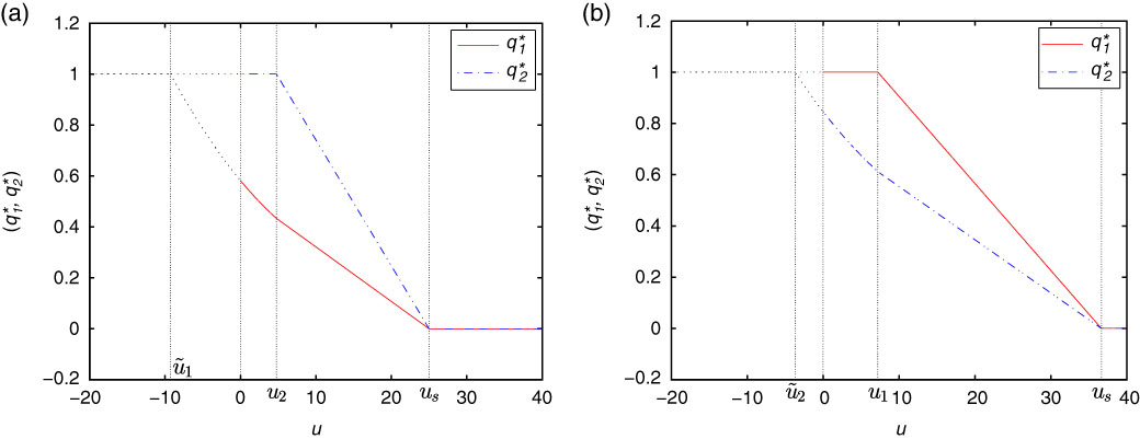
Figure 1 The influence of u on the optimal reinsurance strategy.

From Figure 1, we can see that the optimal reinsurance strategy $\left( {q_{1}^{{\rm {\asterisk}}} ,q_{2}^{{\rm {\asterisk}}} } \right)$ decreases as u increases. It is to be expected, since, according to (3.1) and (3.6), we can prove that $q_{1}^{{\rm {\asterisk}}} $ and $q_{2}^{{\rm {\asterisk}}} $ are decreasing and continuous functions w.r.t. u. Furthermore, we can observe from Figure 1(a) that $q_{1}^{{\rm {\asterisk}}} $ is always less than $q_{2}^{{\rm {\asterisk}}} $ when the two lines have the same safety loading for insurer as well as for reinsurer, say, η ₁=η ₂=0.22. It is also natural consequence since the insurer always tries to keep a smaller retention level for the heavy-tailed risk business. However, when the reinsurer’s safety loading in the first line is much larger than the one in the second, say, η ₁=0.4 and η ₂=0.15, it is reasonable for the insurer to keep a smaller retention level for the cheaper one (see Figure 1(b)).

Figure 2 The influence of m and λ on the minimum probability of drawdown.

Figure 2 shows that the minimum probability of drawdown ϕ(u,m) satisfies the boundary conditions: ϕ(am,m)=1 and ϕ(u _s ,m)=0. Besides, we can see that ϕ(u,m) is a decreasing function w.r.t. u but an increasing function w.r.t. m and λ. They are natural consequences, since, when the value of the surplus increases toward u _s , the insurer can transfer all the risk to reinsurer, and thus the wealth will never decrease, then drawdown cannot happen. However, the drawdown level increases as the maximum (past) value m increases (See Figure 2(a)), and a greater value of λ means a greater value of expected claim number as well as safe level, which both could make drawdown more likely (See Figure 2(b)).

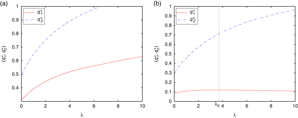
Figure 3 The influence of λ on the optimal reinsurance strategy.

From Figure 3(a) with η ₁=0.25 and η ₂=0.2, we can see that the optimal reinsurance strategy increases when λ increases, which implies that even though the greater value of λ means a greater value of expected claim number, the insurer still chooses to retain a larger share of each claim because of the expensive reinsurance cost. However, when the reinsurance premium is small enough, the insurer would rather retain a less share of the claim when the expected claim number becomes larger. This kind of property is shown in Figure 3(b) with η ₁=0.14 and η ₂=0.25, where a greater value of λ(>λ ₀) yields a less value of the optimal reinsurance strategy $q_{1}^{{\rm {\asterisk}}} $ . Besides, it is not difficult to see that the optimal reinsurance strategy $q_{2}^{{\rm {\asterisk}}} $ in Figure 3(a) increases faster than the one in Figure 3(b) when λ increases, which shows once more that the reinsurer’s safety loading has a direct impact on the optimal reinsurance strategy.

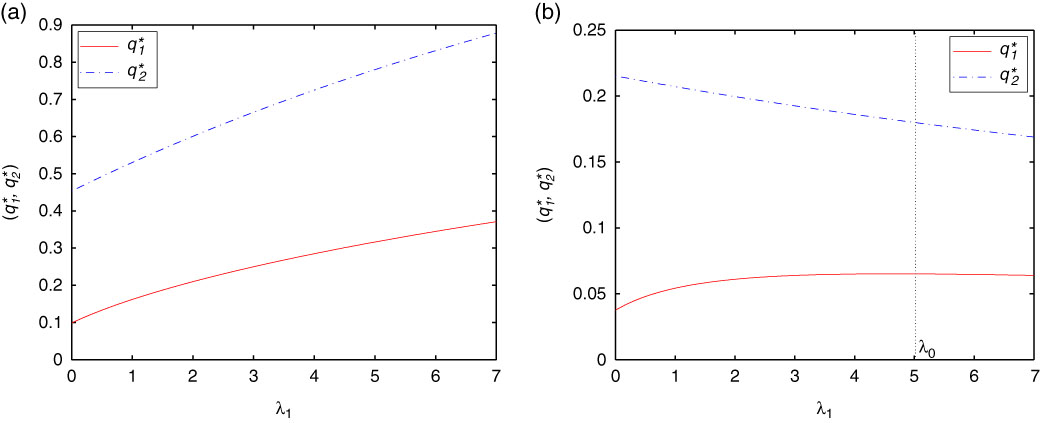
Figure 4 The influence of λ ₁ on the optimal reinsurance strategy.

From Figure 4(a) with η ₁=0.21 and η ₂=0.23, we can see that a greater value of λ ₁ yields greater values of the optimal reinsurance strategy $q_{1}^{{\rm {\asterisk}}} $ and ${\rm q}_{2}^{{\rm {\asterisk}}} $ . It makes sense because the reinsurance premium is much more expensive in this case, the insurer would rather retain a larger share of each claim even though a greater value of λ ₁ implies a larger insurance risk. However, when the reinsurer’s safety loading is small enough, say η ₁=0.1 and η ₂=0.12 as in Figure 4(b), to reduce the risk, the insurer tends to purchase more reinsurance for class 2 because of the cheap reinsurance premium. Meanwhile, since $q_{1}^{{\rm {\asterisk}}} $ is much more sensitive to λ ₁ than $q_{2}^{{\rm {\asterisk}}} $ , there is a trade-off in allowing q ₁ to increase or decrease. When λ ₁ is not large enough, say λ ₁<λ ₀, the insurer prefers to retain a greater share of each claim as λ ₁ increases, which could help increase the premium income. However, a greater value of λ ₁ also implies a larger insurance risk, when λ ₁ is large enough, say λ ₁>λ ₀, the insurer needs to reduce the risk of its insurance portfolios by transferring more risk to the reinsurer.

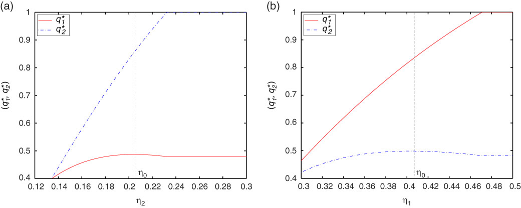
Figure 5 The influence of η ₁ and η ₂ on the optimal reinsurance strategy.

Figure 5 further investigates the influence of the reinsurer’s safety loadings, i.e., η ₁ and η ₂ on optimal reinsurance strategy. It is easy to see that a greater value of η _i (i=1,2) yields a greater value of $q_{i}^{{\rm {\asterisk}}} (i{\equals}1,2)$ , which illustrates the intuitive observation that if the reinsurance premium increases, the insurer would rather retain a greater share of each claim by purchasing less reinsurance. We also see that as the value of η ₁(η ₂) increases, the retention level of the other class first increases and then decreases after reaching a certain level (say, η ₀). These observations are kind of reasonable. When the company keep buying less and less reinsurance for one class, it eventually needs to reduce the risk of its insurance portfolios by buying a bit more reinsurance for another class.