


1. Introduction
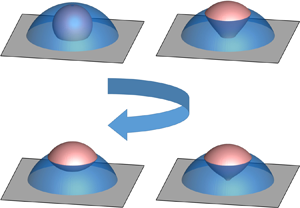
Compound sessile drops have gained considerable attention due to their potential uses in pharmaceutical formulations (Zarzar et al. Reference Zarzar, Sresht, Sletten, Kalow, Blanschtein and Swager2015), drug delivery (Sundararajan et al. Reference Sundararajan, Wang, Rosen, Procopio and Rosenberg2017) and inkjet printing (Keller et al. Reference Keller, Yakovlev, Grachova and Vinogradov2018). Here, the compound sessile drops refer to the drops comprised of two or more immiscible fluids and sticking to a plate substrate. The geometry of compound sessile drops at equilibrium is of great importance in industrial applications, and can exhibit a variety of complicated morphological configurations. The multiphase system involving ternary fluids in contact with a solid in figure 1 shows a good example, and it is also the focus of present paper. In this system, a compound sessile drop consisting of two fluids is immersed in a third, mutually immiscible liquid, and the morphological configurations include encapsulation, lens, collars and Janus, to name but a few. They are distinguishable by the relative position of the component droplets of the compound drop and whether the component droplets are in contact with the substrate.

Figure 1. Morphological configurations of compound sessile drops resting on a flat substrate: (a) encapsulation, (b) lens, (c) collars and (d) Janus, which are also referred thereafter to as configurations  $E$,
$E$,  $L$,
$L$,  $C$ and
  $J$, respectively. Solid lines represent the surface of the component droplet 1 (made up of fluid 1), while dashed lines represent the surface of the component droplet 2 (made up of fluid 2).
For each configuration, the geometry of the compound sessile drop at the equilibrium state is generally dictated by the minimization of the system energy, or more precisely, is related to the physical parameters including interfacial tensions, wettability of the substrate, volume of the compound drop, volume ratio of the two component droplets and gravity. Based on the Young–Laplace equation, Mahadevan, Assa-bedia & Pomeau (Reference Mahadevan, Assa-bedia and Pomeau2002) provided the analytical expression of geometrical relations in the absence of gravity for two configurations of compound sessile drops, i.e. encapsulation and lens. Neeson et al. (Reference Neeson, Tabor, Grieser, Dagastine and Chan2012) presented a theoretical description of the drop geometry in the collars configuration, for compound sessile drops with negligible gravitational effect. Furthermore, their theoretical prediction of the drop shape at equilibrium in the collars configuration was found to agree well with that in experiments, in particular when the compound sessile drops are significantly below the capillary length. Li et al. (Reference Li, Del Hierro, Di and Zuo2020a) theoretically investigated the equilibrium shape of a pendent compound droplet in the lens configuration, on which the gravitational force plays an important role. On the other hand, it is noteworthy that given the physical parameters for a compound sessile drop, its geometry at equilibrium cannot be uniquely determined. This is mainly due to the fact that multiple configurations could be stable for the same fluid parameters. Therefore, the configuration of a compound sessile drop depends on the way of generating it.
It has been reported in experiments that the transition between the morphological configurations might occur when the fluid parameters were changed. Neeson et al. (Reference Neeson, Tabor, Grieser, Dagastine and Chan2012) found that if one component of a compound sessile drop can evaporate, the resulting change of the volume ratio can lead to the configuration transition, e.g. from Janus to collars or from lens to collars. Iqbal et al. (Reference Iqbal, Dhiman, Sen and Shen2017) further studied the suspension of small oil droplets at the top of the water droplets for a variety of volume ratios between the oil and water droplets, and observed that there exists a critical volume ratio, above which the lens configuration would transit to Janus. Bansal & Sen (Reference Bansal and Sen2017) actuated the oscillations of concentric compound drops of water surrounded by an oil shell using electrowetting, which promotes the configuration transition from encapsulation to collars. To assess the onset of configuration transition from the theoretical point of view, Mahadevan et al. (Reference Mahadevan, Assa-bedia and Pomeau2002) presented a geometrical criterion, i.e. the merging of four phases along a single contact line in the encapsulation configuration, which would lead to the configuration transition from encapsulation to lens. These findings suggest the potential of controlling the configuration transition and reconfiguring the compound sessile drops in industrial applications. However, it needs systematic studies to identify all the critical conditions for the configuration transition to occur, and to determine the configuration and geometry of the compound sessile drops at equilibrium after the configuration transition takes place.
In this paper, we investigate the configuration transitions of compound sessile drops by theoretical analysis and numerical simulations, in particular among the axisymmetric configurations, i.e. encapsulation, lens and collars. In the present study, we do not consider the effect of gravity, as the size of the drops considered is much smaller than the capillary length. Here, the capillary length for the ternary fluids is defined as  $l_c=\min \{ \sqrt {{\sigma _{ij}}/{|\rho _i-\rho _j|g}}\}$, where
  $\rho _i$ and
  $\rho _j$ are the density of the fluid
  $i$ and fluid
  $j$, respectively,
  $g$ the gravity,
  $\sigma _{ij}$ the interface tension coefficient between the fluid
  $i$ and fluid
  $j$, the subscripts
  $\{i, j\} = \{1, 2, 3\}$ and
  $i\ne j$. The substrate is assumed to be very smooth and chemically homogeneous, and thus the effect of contact angle hysteresis is also neglected. The configuration transitions are caused by varying the wettability of the substrate (specifically
  $\theta _{23}$, which exists in all the configurations, see figure 1d) and the volume ratio of the two component droplets (
 $\lambda$), in the range of
  $\lambda \in [0, 1]$ and
  $\theta _{23} \in [55^{\circ }, 125^{\circ }]$. The geometry of the compound sessile drop at equilibrium in the respective configurations is obtained by solving the related interface equations derived from the Young–Laplace equation. Here, the initial state is very important in solving the interface equations, since different final states could be reached from different initial states. A ternary-fluid diffuse-interface method is used to simulate the dynamics of configuration transition, and to examine the eventual configuration and geometry of the drop. The theoretical analysis allows us to evaluate the criteria for the onset of configuration transition, establish the boundaries in the parameter space within which the respective configuration can hold, and identify the irreversible and reversible configuration transitions. In particular, we find that the geometrical criteria are not sufficient to describe the configuration transitions. With the help of numerical simulations, we reveal the dynamic behaviours of configuration transitions that are not accessible to theoretical analysis, and assess the theoretical prediction of the drop geometry at equilibrium after the occurrence of configuration transition. Furthermore, we discuss the feasibility in the controllable reconfiguration of the compound sessile drops, and also provide a theoretical way of how to achieve this ultimate purpose.
2. Problem statement and methodology
2.1. Problem statement
We investigate here the configuration transition of compound sessile drops on a flat substrate, in which the compound sessile drop consists of two immiscible fluids, immersed in a third one. We mainly concentrate on the axisymmetric configurations of the compound sessile drop, including encapsulation, lens and collars, namely configurations  $E$,
$E$,  $L$ and
  $C$, respectively; a sketch of these configurations can be seen in figure 1(a–c). These configurations of compound sessile drops are primarily defined according to the relative position of its component droplets and whether the component droplets are in contact with the substrate. In the encapsulation configuration, the droplet of fluid 1 (namely droplet 1) is wrapped by the droplet of fluid 2 (namely droplet 2) in an axisymmetric manner, and both droplets are in contact with the substrate (figure 1a). In the lens configuration, droplet 1 floats on the top of droplet 2 that is in contact with the solid substrate (figure 1b). In the collars configuration, droplet 1 is partially immersed in droplet 2, and both droplets are in contact with the substrate (figure 1c). In each configuration, the relative significance of droplet volume can be measured by the volume ratio of droplet 1 to the compound drop,
  $\lambda$, and thus the volume ratio of droplet 2 is
  $1-\lambda$. It is noteworthy that the positions of fluid 1 and fluid 2 can be swapped in the configurations listed in figure 1(a–c).
The compound sessile drops considered are supposed to be sufficiently small so that the gravitational force can be neglected. Therefore, the force balance between the interface tensions among the fluids and the substrate dictates the shape of the compound drop at equilibrium. The interface tension coefficients between the fluids are assumed to satisfy the triangular inequality,  $\sigma _{ij}<\sigma _{jk}+\sigma _{ki}$, for all cyclic permutations of the indices
  $\{i, j, k\} = \{1, 2, 3\}$. In such a case, the relative significance of the interface tensions between the fluids can be represented by the interfacial angles (
 $\varphi _1$,
  $\varphi _2$ and
  $\varphi _3$ in figure 1(d), and
  $\varphi _1+\varphi _2+\varphi _3 = 360^{\circ }$) at the triple-phase line where the ternary fluids meet. Specifically, they are associated with the interface tensions by Neumann's triangle (Mahadevan et al. Reference Mahadevan, Assa-bedia and Pomeau2002),
 \begin{equation} \frac{\sin\varphi_1}{\sigma_{23}} = \frac{\sin\varphi_2}{\sigma_{31}} = \frac{\sin\varphi_3}{\sigma_{12}}. \end{equation}
 For a compound sessile drop at equilibrium, Young's equation suggests  $\sigma _{ij}\cos \theta _{ij}=\sigma _{js}-\sigma _{is}$, where
  $\sigma _{js}$ (
 $\sigma _{is}$) denotes the interface tension between the fluid
  $j$ (
$j$ ( $i$) and the substrate. The static contact angle
  $\theta _{ij}$ corresponds to the angle that the interface between fluids
  $i$ and
  $j$ intersects with the substrate, particularly measured from the side of fluid
  $i$ – geometrically,
  $\theta _{ij}+\theta _{ji}=180^{\circ }$ (see figure 1d). Combining Young's equation with Neumann's triangle, we can get that the interfacial angles and the contact angles should yield the following constraint (Zhang et al. Reference Zhang, Ding, Gao and Wu2016):
 \begin{equation} \sin\varphi_2 \cos\theta_{13} -\sin\varphi_3 \cos\theta_{12} - \sin\varphi_1 \cos\theta_{23} = 0. \end{equation}
 From the analysis above, we can see that the geometry of the compound sessile drop with specific configuration can be uniquely determined, given the volume ratio  $\lambda$, the interfacial angles (
 $\varphi _1$,
  $\varphi _2$ and
  $\varphi _3$) and any two contact angles in (2.2). The interface tension coefficients are fixed for the convenience of analysis, more specifically,
  $\sigma _{12}: \sigma _{23}: \sigma _{31}=1: \sqrt {3}: 2$, which corresponds to the interfacial angles of
  $\varphi _1=120^{\circ }$,
  $\varphi _2=90^{\circ }$ and
  $\varphi _3=150^{\circ }$. Similarly, we set
  $\sigma _{1s}=\sigma _{3s}$, leading to
  $\theta _{13}=90^{\circ }$. Thus, it is easy to obtain from (2.2) that
 \begin{equation} \cos\theta_{12}={-}\frac{\sigma_{23}}{\sigma_{12}}\cos\theta_{23}={-}\sqrt{3} \cos\theta_{23}. \end{equation}
Note that the contact angle  $\theta _{12}$ is allowed to vary from
  $0^{\circ }$ to
  $180^{\circ }$. Consequently, the range of
  $\theta _{23}$ is restricted to [
 $55^{\circ }$,
  $125^{\circ }$]. Consequently, for a specific compound drop, the configuration of the compound sessile drop at equilibrium depends only on
  $\lambda$ and
  $\theta _{23}$.
2.2. Theoretical prediction of drop geometry
In this section, we present the governing equations and boundary conditions for the theoretical prediction of the geometry of the compound sessile drop. For a compound sessile drop at equilibrium, there is a force balance between Laplace excess pressure and surface tension across any of its interface, which yields
 \begin{equation} p_i-p_j=\sigma_{ij}\left(\frac{1}{R_1}+\frac{1}{R_2}\right), \end{equation}
where  $p_i$ and
  $p_j$ denote the constant pressure of the fluids
  $i$ and
  $j$, respectively, and
  $R_1$ and
  $R_2$ represent the two principal radii of interface curvature.
The interfaces of the compound drop are described in a curvilinear coordinate ( $x, \phi$), where
  $x$ is the distance from any point on the interface to the symmetry axis, and
  $\phi$ is the angle between the interface tangent and the horizontal direction (figure 1b). As a result, the principal radii of curvature can be represented in terms of
  $x$ and
  $\phi$,
 \begin{equation} R_{1}= \frac{1}{\cos\phi}\frac{\textrm{d}x}{{\textrm{d}}\phi} \quad \text{and}\quad R_{2}= \frac{x}{\sin\phi}. \end{equation}
Substituting (2.5a,b) into (2.4) and defining the interface curvature as  $M=(p_i-p_j)/\sigma _{ij}$, we can obtain
  $M= \cos \phi \cdot {{\textrm {d}}\phi }/{\textrm {d}x}+{\sin \phi }/{x}$. Integration of this equation over any interface that separates two fluids gives (Carroll Reference Carroll1976)
 \begin{equation} x\sin\phi =\tfrac{1}{2} M x^{2}+ N, \end{equation}
where  $N$ is an integration constant associated with
  $M$ and the boundaries of the interface.
Equation (2.6) provides a description of interface shapes in the coordinate ( $x$,
$x$,  $\phi$). To determine the shape of the compound sessile drop at equilibrium, the boundary conditions of the interfaces, i.e. the starting point (
 $x_s$,
  $\phi _s$) and the end point (
 $x_e$,
  $\phi _e$), and the interface parameters
  $M$ and
  $N$ should be explicitly obtained for every interface of compound sessile drops. In principle, these parameters are a function of
  $\lambda$, interface angles and contact angles, and can be determined by taking account of the geometrical and physical constraints, such as the drop volume and the force balance. Once these parameters are obtained, the rescaled surface energy of the compound sessile drop,
  $E_S$, can be calculated – see more details in the Appendix A.
The solutions of the interfaces for compound sessile drops are obtained by using a shooting method and a binary searching method. Because of the presence of the triple-phase line in the latter, the governing equations of the three interfaces are strongly coupled, and are thus solved simultaneously. For the spherical interfaces, the analytical solution of the interface can be obtained and explicitly expressed in terms of  $x$ and
  $\phi$. However, for the non-spherical interfaces, one additional constraint is required to determine the interface shape. In this case, the interface geometry can only be obtained numerically.
2.3. Ternary-fluid diffuse-interface model
A ternary-fluid diffuse-interface model is coupled with Navier–Stokes equations (Zhang et al. Reference Zhang, Ding, Gao and Wu2016), to simulate the dynamic process of configuration transition of a compound sessile drop on a flat substrate. The total volume of the compound drop is denoted by  $V_0$, which also gives rise to a characteristic length
  $R=\sqrt [3]{0.75V_0/{\rm \pi} }$. The ternary fluids are assumed to have the same viscosity
  $\mu$ and density
  $\rho$. To compare with the theoretical prediction, the transition is ideally quasi-static in the numerical simulation. That is, viscosity is dominant over the inertia and surface tension of the compound sessile drop, so as to suppress the capillary waves induced by configuration transition. Therefore, it is appropriate to use a large Ohnesorge number (
 $Oh=\mu /\sqrt {\rho R \sigma _{13}}$), and
  $Oh=0.1$ is considered to be sufficiently large for this purpose. Numerical results can be very helpful in determining whether the theoretical analysis produces physically meaningful solutions. Unless otherwise stated, all the times of numerical results have been rescaled by the capillary time
  $\sqrt {\rho R^{3}/\sigma _{13}}$.
In the ternary-fluid diffuse-interface model, the interfaces are represented by the contours of the volume fractions of the fluids 1 and 2, i.e.  $C_1$ and
  $C_2$, respectively. The interface evolution can be tracked by
 \begin{equation} \frac{\partial \textbf{C}} {\partial t} + \boldsymbol{\nabla} \boldsymbol{\cdot} ({\boldsymbol uC}) = \frac{1}{Pe}\nabla^{2} {\boldsymbol\varPsi}, \end{equation}
where  $\textbf {C}=(C_1, C_2)$ and
  $\textbf {u}$ is the flow velocity. The chemical potential
  ${\boldsymbol \varPsi }=(\varPsi _1, \varPsi _2)$ is defined as
 \begin{equation} {\varPsi_i} = C_i^{3}-1.5C_i^{2}+0.5C_i-C_1C_2(1-C_1-C_2) - Cn ^{2} \nabla^{2} {C_i},\quad i=1\ \textrm{or}\ 2, \end{equation}
where the Cahn number is set to  $Cn=0.7h/R$, the Péclet number is set to
  $Pe=1/Cn$ (Liu & Ding Reference Liu and Ding2015) and
  $h$ is the mesh size. More details in the numerical implementation can be found in Zhang et al. (Reference Zhang, Ding, Gao and Wu2016).
Axisymmetric simulations are performed in a domain of  $3R \times 2R$ on a uniform Cartesian grid of
  $600\times 400$, i.e.
  $h=0.005R$. The boundary conditions are: symmetry condition at the left boundary; solid wall condition at the bottom boundary; and extrapolation condition at the upper and right boundaries. The same code was used to obtain the equilibrium states of two-dimensional Janus drops on a flat substrate and a compound droplet inside a capillary (Zhang et al. Reference Zhang, Ding, Gao and Wu2016), and good agreement with the theoretical prediction of drop geometries has been achieved. In the present study, numerical simulations are also used to verify the theoretical prediction of the configurations
  $E$,
$E$,  $L$ and
  $C$, since the theoretical prediction could lead to non-physical solutions (see more details in § 3.1). For the physical solutions, the theoretical prediction is expected to be virtually overlapped with the numerical results, with respect to the shape of compound sessile drops at equilibrium. Examples are shown in figure 2, with different volume ratio
  $\lambda$ and contact angles
  $\theta _{23}$.

Figure 2. Verification of theoretical predictions of compound sessile drops at equilibrium. (a) Configuration  $E$ with
  $\lambda =0.100$ and
  $\theta _{23}=70^{\circ }$. (b) Configuration
  $L$ with
  $\lambda =0.250$ and
  $\theta _{23}=80^{\circ }$. (c) Configuration
  $C$ with
  $\lambda =0.400$ and
  $\theta _{23}=70^{\circ }$. (d) Configuration
  $C$ with
  $\lambda =0.400$ and
  $\theta _{23}=100^{\circ }$. Solid lines are the numerical results and dashed lines are the theoretical prediction.
3. Phase diagram of compound sessile drops
We present here the phase diagram of the compound drop configurations in the parameter space of  $\lambda \in [0, 1]$ and
  $\theta _{23} \in [55^{\circ }, 125^{\circ }]$. The solutions are obtained by theoretical analysis, consisting of encapsulation (§ 3.2), lens (§ 3.3) and collars (§ 3.1). For simplicity, the interface between the fluids
  $j$ and
  $k$ is referred to as
  $I_{jk}$, and accordingly, the geometry parameters for
  $I_{jk}$ in (2.6) are denoted by
  $(M_i, N_i)$, with cyclic permutations of the indices
  $\{i, j, k\} = \{1, 2, 3\}$.
3.1. Collars
A compound sessile drop with configuration  $C$ consists of three interfaces as shown in figure 3(a), among which the boundary conditions of
  $I_{23}$ and
  $I_{13}$ are:
  $\phi |_{x=r_1}=\theta _{23}$ and
  $\phi |_{x=r_2}=\varphi _3+\alpha -180^{\circ }$ for
  $I_{23}$; and
  $\phi |_{x=r_2}=\alpha$ and
  $\phi |_{x=0}=0$ for
  $I_{13}$. For
  $I_{12}$, the boundary conditions are
  $\phi |_{x=r_3}=\theta _{12}$ and
  $\phi |_{x=r_2}=180^{\circ }-\varphi _1+\alpha$, where
  $r_3$ is the radius of contact line of droplet 1. With these boundary conditions, we can get the interface parameters
 \begin{gather} \left.\begin{gathered} \displaystyle M_1=\frac{2(r_1 \sin\theta_{23}+r_2 \sin(\varphi_3+\alpha))}{r_1^{2}-r_2^{2}}, \\ \displaystyle N_1=\frac{-r_1 r_2(r_1 \sin(\varphi_3+\alpha)+r_2 \sin\theta_{23})}{r_1^{2}-r_2^{2}}, \end{gathered}\right\} \end{gather}
 \begin{gather} \left.\begin{gathered} \displaystyle M_2=\frac{2\sin\alpha}{r_2}, \\ \displaystyle N_2=0 \end{gathered}\right\}\end{gather}
and
 \begin{equation} \left.\begin{gathered} \displaystyle M_3=\frac{2(r_3 \sin\theta_{12}-r_2 \sin(\varphi_1-\alpha))}{r_3^{2}-r_2^{2}}, \\ \displaystyle N_3=\frac{r_2 r_3(r_3 \sin(\varphi_1-\alpha)+r_2 \sin\theta_{12})}{r_3^{2}-r_2^{2}}. \end{gathered}\right\} \end{equation}
It is noteworthy that an interface with  $N=0$ assumes a shape of spherical cap, and consequently, the radius of the spherical cap is
  $2/M$. Thus, among the interfaces in configuration
  $C$, either
  $I_{12}$ or
  $I_{23}$ does not assume a spherical shape, but
  $I_{13}$ does. To simplify the computation of
  $M$ and
  $N$, we consider the balance between the Laplace pressures
 \begin{equation} M_1 \sigma_{23}-M_2 \sigma_{13}+M_3 \sigma_{12}=p_2-p_3-(p_1-p_3)+(p_1-p_2)=0. \end{equation}
Figure 3. Geometry and configuration boundaries of configuration  $C$. Panel (a) shows the general drop shape of configuration
  $C$ with
  $\theta _{23}= 80^{\circ }$ and
  $\lambda =0.500$. The drop shapes at the critical conditions are shown in panel (b)
  $\theta _{23}=70^{\circ }$ and
  $\lambda =0.341$ and panel (c)
  $\theta _{23}= 100^{\circ }$ and
  $\lambda =0.267$). Panel (d) shows the regime diagram with respect to
  $\lambda$ and
  $\theta _{23}$, in which the grey indicates the region where the configuration
  $C$ is stable. The boundaries are represented by three critical volume ratios:
  $\lambda _{c,1}$ (at which
  $r_3$ reaches a minimum value below which there is no solution for configuration
  $C$),
$C$),  $\lambda _{c,2}$ (at which
  $r_2$ reaches a minimum value) and
  $\lambda _{c,3}$ (at which
  $r_1=r_3$).
In the expressions (3.1)–(3.3), there are four unknowns:  $\alpha$;
  $r_1$;
  $r_2$; and
  $r_3$. In addition to the three constraints, i.e. the volumes of droplets 1 and 2, and the force balance (3.4), it is necessary to have one more constraint to uniquely determine the four unknowns. Here, the additional constraint is a geometrical one, i.e.
  $I_{12}$ and
  $I_{23}$ have the same height, which can be expressed as
 \begin{equation} \left|\int_{r_1}^{r_2} \tan\phi_1 \,{\textrm{d}}x_1\right| =\left|\int_{r_3}^{r_2} \tan\phi_3 \,{\textrm{d}}x_3\right|. \end{equation}
To get  $\alpha$,
  $r_1$,
  $r_2$ and
  $r_3$, a shooting method is used to find the solutions that satisfy the constraints, along with a fourth-order Runge–Kutta scheme to approximate the integration.
The phase boundaries of configuration  $C$ heavily relies on the value of
  $\theta _{23}$. We note that
  $\theta _{23}$ and
  $\theta _{21}$ (
 $=180^{\circ } - \theta _{12}$) are similar, in the sense that they both are acute angles (see e.g. figure 3b) or obtuse angles (see e.g. figure 3c) at the same time according to (2.3). It is natural to expect from a geometrical point of view that configuration transition would not occur unless the contact line of
  $I_{12}$ moves inwards and meets at the
  $z$-axis for
  $\theta _{23}<90^{\circ }$, i.e.
  $r_3=0$; similarly, it is expected for
  $\theta _{23}>90^{\circ }$ that either the vanishing of
  $I_{13}$ (i.e.
  $r_2=0$) or the merging of the contact lines of
  $I_{23}$ and
  $I_{12}$ on the substrate (i.e.
  $r_1=r_3$) could lead to the occurrence of configuration transition. However, our theoretical solutions suggest that these geometrical conditions do not correspond to the transition boundaries of configuration
  $C$.
$C$.
Figure 4(a) shows the solution at  $\theta _{23}=70^{\circ }$ in terms of
  $r_3$ versus
  $\lambda$. Firstly, we can see that there exists a minimum value of
  $r_3$, i.e.
  $r_{3,min}=0.233$ at
  $\lambda _{c, 1}=0.345$, below which there is no solution for configuration
  $C$. In other words, configuration transition for
  $\theta _{23}<90^{\circ }$ occurs much earlier than the prediction of geometrical condition, i.e.
  $r_3=0$. Secondly, we observe that configuration
  $C$ might have multiple solutions with the same parameters. For example, there are two solutions of compound sessile drops in the configuration
  $C$ at
  $\lambda =0.6$:
  $r_3=0.601$ and
  $r_3=0.030$, of which the drop shapes are shown in figures 4(b) and 4(d), respectively. Our numerical simulation indicates that an initial set-up of a drop with
  $r_3=0.030$ is unstable and gradually transits to the equilibrium state with
  $r_3=0.601$ (figure 4e). The variation of the rescaled surface energy
  $E_S$ with
  $\theta _{23}=70^{\circ }$ is also shown in figure 4(a). We can see that the surface energy of the drop shape in figure 4(d) is higher than that of figure 4(b), and the lowest surface energy occurs at
  $r_3=r_{3,min}$. In fact, the theoretical prediction of configuration
  $C$ at
  $\theta _{23}=70^{\circ }$ is a saddle-point bifurcation, and has two branches of solutions – see figures 4(a). The turning point (
 $r_3=r_{3,min}$ and
  $\lambda _{c, 1}=0.345$) separating the unstable solutions (the lower branch) from the stable ones (the upper branch) also represents the phase boundary at
  $\theta _{23}=70^{\circ }$. In other words, the saddle-point bifurcation represents another type of criteria for the onset of configuration transition, in addition to the geometrical criteria. In such a way, we can theoretically predict the phase boundary of configuration
  $C$ at
  $\theta _{23}<90^{\circ }$, which is included in figure 3(d).

Figure 4. Saddle-point bifurcation in the solution of configuration  $C$. (a) Contact line position
  $r_3$ (solid lines) and the rescaled system energy
  $E_S$ (dashed lines) at
  $\theta _{23}=70^{\circ }$ as a function of volume ratio
  $\lambda$. (b) One theoretical prediction of the drop geometry with
  $\lambda =0.600$ and
  $r_3=0.601$ (denoted by
  $\blacksquare$ in panel (a)). (c) The drop geometry at the onset of configuration transition at
  $\lambda =0.345$ and
  $r_3=0.233$ (denoted by
  $\bullet$ in panel (a)). (d) The non-physical theoretical prediction of the drop geometry with
  $\lambda =0.600$ and
  $r_3=0.601$ (denoted by
  $\blacktriangle$ in panel (a)). (e) Temporal evolution of the drop geometry from panel (d) to panel (b) obtained by numerical simulations. The arrow indicates the sequence of the times.
Also due to the occurrence of the saddle-point bifurcation, the geometrical condition  $r_2=0$ for
  $\theta _{23}>90^{\circ }$ underestimates the value of
  $r_2$ at onset of configuration transition. The solution of the phase boundary is plotted in terms of
  $\lambda _{c, 2}$ versus
  $\theta _{23}$ in figure 3(d). In addition, the third critical condition for configuration
  $C$, i.e.
  $r_1=r_3$, has effects on the configuration transition for
  $\theta _{23}>90^{\circ }$ too (denoted by
  $\lambda _{c, 3}$ versus
  $\theta _{23}$ in figure 3d), thereby leading to the phase boundary in this range of
  $\theta _{23}$ consisting of two curves.
The effect of changing interface tension coefficients on the phase boundaries can also be qualitatively analysed here. The change of any interface tension coefficient among  $\sigma _{12}$,
  $\sigma _{13}$ and
  $\sigma _{23}$ would result in the variation of the interface angles and the interface curvatures
  $M$ (see also (3.4)), thereby causing the position change of the triple-phase line. Therefore, we can expect that the phase boundaries would be changed accordingly, but the pattern should be similar. For example, around
  $\theta _{23}=90^{\circ }$, the phase boundaries are represented by
  $\lambda _{c, 1}$ (for
  $\theta _{23}<90^{\circ }$) and
  $\lambda _{c, 2}$ (for
  $\theta _{23}>90^{\circ }$), respectively. The slope of
  $I_{12}$ accounts for this sharp change in the phase boundaries, in the sense that it determines which would firstly intersect with the axis of symmetry: the moving contact line or the triple-phase point. As a result, a sharp change in the phase boundaries always occurs at
  $\theta _{12}=90^{\circ }$ (or equivalently,
  $\theta _{23}=90^{\circ }$ according to (2.3)), regardless of the variation of interface tension coefficients.
3.2. Encapsulation
A typical compound sessile drop with configuration  $E$ is showed in figure 5(a). The compound sessile drop has two interfaces, i.e.
  $I_{12}$ and
  $I_{23}$, characterized by the radius of the wetted area, i.e.
  $r_3$ and
  $r_1$, respectively. Therefore, the boundary conditions are:
  $\phi |_{x=r_3}=\theta _{12}$ at the contact line and
  $\phi |_{x=0}=0$ at the symmetry axis for
  $I_{12}$; and
  $\phi |_{x=r_1}=\theta _{23}$ at the contact line and
  $\phi |_{x=0}=0$ at the symmetry axis for
  $I_{23}$. The interface shapes at equilibrium can be solved by taking these boundary conditions into account. Specifically, we can get
  $(M_3, N_3)=(2\sin \theta _{12}/r_3, 0)$ and
  $(M_1, N_1)=(2\sin \theta _{23}/r_1, 0)$. Thus, both
  $I_{12}$ and
  $I_{23}$ are spherical caps. From the calculation of drop volume, it is easy to associate
  $r_3$ and
  $r_1$ with
  $\lambda$ and contact angles
 \begin{equation} \frac{r_3}{R}=\sqrt[3]{\frac{4\lambda}{V(\theta_{12})}}\quad \text{and}\quad \frac{r_1}{R}=\sqrt[3]{\frac{4}{V(\theta_{23})}}, \end{equation}
where the function  $V$ is defined as
  $V(\xi )=(1-\cos \xi )^{2} (2+\cos \xi )/\sin ^{3}\xi$.

Figure 5. Geometry and configuration boundaries of configuration  $E$. Panel (a) shows the drop geometry with
  $\theta _{23}= 80^{\circ }$ and
  $\lambda =0.100$, panels (b,c) represent the geometrical criteria for the occurrence of configuration transition, and panel (d) shows the regime diagram with respect to
  $\lambda$ and
  $\theta _{23}$, in which the grey indicates the region where the configuration
  $E$ is stable. The boundaries correspond to the two critical volume ratios:
  $\lambda _{c,1}$ (solid line) and
  $\lambda _{c,2}$ (dashed line), respectively.
With the variation of  $\lambda$ and/or
  $\theta _{23}$, the two interfaces may come into contact – see e.g. figures 5(b) and 5(c). Occurrence of configuration transition can be expected in these cases, thereby defining the phase boundary of configuration
  $E$. The contact of the interfaces would occur at the top of the drop when
  $\theta _{23}<\theta _{12}$ (figure 5b), or at the contact line when
  $\theta _{23}>\theta _{12}$ (figure 5c). Mathematically, the phase boundaries can be expressed as
  $r_3(1-\cos \theta _{12})/\sin \theta _{12}=r_1(1-\cos \theta _{23})/\sin \theta _{23}$ in the former, and
  $r_1=r_3$ in the latter, which is consistent with the work of Mahadevan et al. (Reference Mahadevan, Assa-bedia and Pomeau2002). Accordingly, the two phase boundaries can be described with respect to the critical volume ratio,
  $\lambda _{c,1}$ and
  $\lambda _{c,2}$, as a function of the contact angles, by substituting (3.6a,b) into these two conditions. That is,
 \begin{equation} \lambda_{c,1}=\frac{(1-\cos\theta_{23})(2+\cos\theta_{12})}{(1-\cos\theta_{12})(2+\cos\theta_{23})} \quad \text{and}\quad \lambda_{c,2}=\frac{V(\theta_{12})}{V(\theta_{23})}. \end{equation}
 The two boundaries in (3.7a,b) are plotted in figure 5(d) to define the phase diagram of configuration  $E$ with respect to
  $\lambda$ versus
  $\theta _{23}$, of which the result is similar to that of a hollow sessile drop (Gao & Feng Reference Gao and Feng2011). Because of
  $\cos \theta _{12}=-\sqrt {3} \cos \theta _{23}$ in the present study, we can get
  $\lambda _{c,1}=\lambda _{c,2}=1$ at
  $\theta _{23}=90^{\circ }$, which corresponds to
  $\theta _{23}=\theta _{12}$. This implies that the configuration
  $E$ is always stable at
  $\theta _{23}=90^{\circ }$, since the two interfaces are concentrically spherical caps in this case. Furthermore, because the only two interfaces (
 $I_{12}$ and
  $I_{23}$) do not come into contact until the occurrence of configuration transition, the variation of interfacial tension coefficients has no effect on the phase boundaries of configuration
  $E$ (represented by
  $\lambda _{c,1}$ and
  $\lambda _{c,2}$) if the contact angles are fixed.
3.3. Lens
Figure 6(a) shows a typical compound sessile drop with configuration  $L$, of which only
  $I_{23}$ is in contact with the substrate, with the radius of the wetted area denoted by
  $r_1$. The triple-phase line, where three interfaces of the compound drop meet, is also the boundary point shared among the interfaces. Defining the position of the triple-phase line as (
 $r_2, \alpha$) and taking
  $\phi |_{x=0}=0$ at the symmetry axis into account, we can get
  $(M_2, N_2)=(2\sin \alpha /r_2, 0)$. Similarly, the boundary conditions for
  $I_{12}$ can be obtained:
  $\phi |_{x=r_2}=180^{\circ }-\varphi _1+\alpha$ (from geometrical relation at the triple-phase line) and
  $\phi |_{x=0}=180^{\circ }$, leading to the solution of
  $(M_3, N_3)=(2\sin (\varphi _1-\alpha )/r_2, 0)$. Therefore, the interfaces
  $I_{13}$ and
  $I_{12}$ are both spherical caps as
  $N_2=N_3=0$. This fact allows us to relate
  $r_2$ with
  $\lambda$,
  $\varphi _1$ and
  $\alpha$ through the volume formula for a spherical cap
 \begin{equation} \frac{r_2}{R}=\sqrt[3]{\frac{4\lambda}{V(\alpha)+V(\varphi_1 - \alpha)}}. \end{equation}
Figure 6. Geometry and configuration boundaries of configuration  $L$. Panel (a) shows the drop geometry with
  $\theta _{23}= 70^{\circ }$,
  $\lambda =0.300$, panels (b,c) represent the geometrical criteria for the occurrence of configuration transition at
  $(\theta _{23}= 70^{\circ }$,
  $\lambda =0.747$) and
  $(\theta _{23}= 110^{\circ }$,
  $\lambda =0.982$), respectively, and panel (d) shows the regime diagram with respect to
  $\lambda$ and
  $\theta _{23}$, in which the grey indicates the region where the configuration
  $L$ is stable. The boundaries correspond to the two critical volume ratios:
  $\lambda _{c,1}$ (solid line) and
  $\lambda _{c,2}$ (dashed line), respectively.
For  $I_{23}$, the boundary conditions are
  $\phi |_{x=r_1}=\theta _{23}$ at the contact line and
  $\phi |_{x=r_2}=\varphi _3+\alpha -180^{\circ }$ at the triple-phase point. Taking account of the balance between the Laplace pressures (3.4), we can get
  $(M_1,N_1)=(2\sin \theta _{23}/r_1, 0)$ and the radius ratio of
  $r_1$ to
  $r_2$,
 \begin{equation} \eta=\frac{r_1}{r_2}=\frac{-\sin\theta_{23}}{\sin(\alpha+\varphi_3)}. \end{equation}
Thus,  $I_{23}$ is also a spherical cap. Accordingly, the relationship between
  $\alpha$ and
  $\lambda$ can be obtained from volume calculation
 \begin{equation} \lambda=\frac{V(\alpha)+V(\varphi_1-\alpha)}{\eta^{3}V(\theta_{23})+V(\alpha)-V(\alpha+\varphi_3-180^{{\circ}})}= \frac{V(\alpha)+V(120^{{\circ}}-\alpha)}{\eta^{3}V(\theta_{23})+V(\alpha)-V(\alpha-30^{{\circ}})}. \end{equation}
In such a way, all the geometry parameters of the compound sessile drop with configuration  $L$ can be determined by
  $\lambda$, interfacial angles and contact angles. The critical volume ratio
  $\lambda _c$ is directly related to the critical
  $\alpha$ values,
  $\alpha _c$, at which configuration transition occurs.
Figures 6(b) and 6(c) indicate the geometrical criteria for the configuration transition with configuration  $L$, i.e. the occurrence of new contact lines. When
  $\theta _{23}<90^{\circ }$ and
  $I_{12}$ is about to contact the substrate (see e.g. figure 6b), the geometrical criterion for the occurrence of configuration transition is that
  $I_{12}$ and
  $I_{23}$ have the same height. This criterion can be represented by
  $\alpha _{c,1}$,
 \begin{equation} \cos\theta_{23}=\frac{\sin\varphi_2+\sin(\varphi_3+\alpha_{c,1})}{\sin(\varphi_1-\alpha_{c,1})}= \frac{1+\sin(150^{{\circ}}+\alpha_{c,1})}{\sin(120^{{\circ}}-\alpha_{c,1})}. \end{equation}
In case of  $\theta _{23}\ge 90^{\circ }$, the geometrical criterion of configuration transition becomes the vanishing of
  $I_{23}$ and subsequent merging of the four phases at the contact line – see e.g. figure 6(c). Therefore, we can get
  $r_1=r_2$, i.e.
  $-\sin \theta _{23}=\sin (\varphi _3+\alpha _{c,2})$ when taking (3.9) into account. This criterion can be represented by
  $\alpha _{c,2}$, which yields
 \begin{equation} \alpha_{c,2}=\theta_{23}+180^{{\circ}}-\varphi_3=\theta_{23}+30^{{\circ}}. \end{equation}
 Combining (3.11) and (3.10), in principle we can obtain the phase boundaries for configuration  $L$ in terms of
  $\lambda _{c,1}$ versus
  $\theta _{23}$. Similarly, we can also get the phase boundaries of
  $\lambda _{c,2}$. Please note that we cannot obtain the analytical expressions of
  $\lambda _{c, 1}$, but the numerical solutions. The results are plotted in figure 6(d); we can see that configuration
  $L$ is comparably more stable than the other two, with respect to the area of existence in the parameter space of
  $\lambda \in [0, 1]$ and
  $\theta _{23}\ge 90^{\circ }$. Clearly, both
  $\alpha _{c,1}$ and
  $\alpha _{c,2}$ are the function of the interface angles, as seen in (3.11) and (3.10). This suggests that the phase boundaries changes with the interface tension coefficients. In particular, the intersection between
  $\lambda _{c,1}$ and
  $\lambda _{c,2}$ corresponds to
  $\alpha _{c,1}=\alpha _{c,2}=\varphi _1$. Thus, we can obtain from (3.12) that the change in phase boundary happens at
  $\theta _{23}=180^{\circ }-\varphi _2$, which is also a function of the interface angles.
4. Configuration transition of compound sessile drops
4.1. Regime diagram of compound sessile drops
In order to investigate the configuration transition, the phase diagrams of the three configurations (figures 3, 5 and 6) are superimposed to present an overview of coexistence of configurations in figure 7. Several observations can be made of figure 7. Firstly, the phase diagram can be divided into nine zones, among which the zones  $I$,
$I$,  $III$,
  $VII$ and
  $VIII$ include one configuration, the zones
  $II$,
$II$,  $IV$ and
  $VI$ have two, the zone
  $V$ consists of all the three, and the zone
  $IX$ has none. Secondly, if we change
  $\lambda$ or
  $\theta _{23}$ so as to cross the border between two neighbouring zones, the configuration transition might happen, but it is path-dependent. More specifically, it only possibly happens if the border crossing starts from the zone with more configurations to the zone with less. Thirdly, once the configuration transition takes place, it is normally irreversible. It should be emphasized that not all the stable cases in the three configurations have been taken into account in the phase diagram in figure 7. In § 3 we only consider the cases consisting of fluids with relative position illustrated in figure 1(a–c), and thus those cases in which fluid 1 switches the position with fluid 2 are not included.

Figure 7. Superimposed phase diagrams of configurations  $L$,
$L$,  $E$ and
  $C$ with respect
  $\lambda$ to
  $\theta _{23}$.
On the other hand, one may ask what configuration a compound sessile drop would be for specific parameters. To answer this question, it is necessary to know the initial configuration of the drop and the route of parameter change to the specific parameters, which affect the evolution history of geometry and energy of the drop and consequently determine its final state. In the following, we investigate the configuration transitions by a combination of surface energy analysis and numerical simulations.
4.2. History dependence of configuration transition
To show the effect of initial configuration of the drop and the route of parameter change on the configuration transition, we investigate the variation of  $E_S$ as a function of
  $\lambda$, for a fixed value of
  $\theta _{23}$ (
 $=80^{\circ }$). The theoretical prediction of
  $E_S$ as a function of
  $\lambda$ is shown in figure 8(i). At low
  $\lambda$ (
 $=0.1$), two types of compound sessile drops can exist stably, in the configurations
  $E$ (figure 8a) and
  $L$ (figure 8b), respectively. If a compound drop takes the configuration in figure 8(a) as its initial configuration,
  $E_S$ increases monotonically with
  $\lambda$ until a configuration transition occurs (i.e. at
  $\lambda =0.497$, which corresponds to the boundary between the zones
  $V$ and
  $VI$). More precisely, the inside droplet of fluid 1 becomes so big that it starts to touch the interface
  $I_{23}$ (figure 8e), thereby leading to the generation of a new interface, i.e.
  $I_{13}$. We simulate the dynamic process of this configuration transition at
  $\lambda =0.497$, and show the results in figure 9(a), with respect to the snapshots of the drop at different times. It can be seen that after the generation of
  $I_{13}$, the contact line of
  $I_{12}$ moves inwards, and the compound sessile drop gradually evolves into an equilibrium state in configuration
  $C$, of which the shape is well predicted by the theoretical analysis (figure 8f).

Figure 8. Geometry of compound sessile drops and transition among the three configurations at  $\theta _{23}=80^{\circ }$. (a,b) Configurations
  $E$ and
  $L$ at
  $\lambda =0.100$, respectively; (c,d) configurations
  $C$ and
  $L$ at
  $\lambda =0.307$, respectively; (e,f) configurations
  $E$ and
  $L$ at
  $\lambda =0.497$, respectively; (g,h) configurations
  $L$ and
  $C$ at
  $\lambda =0.911$, respectively; (i) surface energy
  $E_S$ as a function of
  $\lambda$.

Figure 9. Snapshots of configuration transition at  $\theta _{23}=80^{\circ }$: (a) from
  $E$ to
  $C$ at the boundary between zone
  $V$ and
  $VI$ (
 $\lambda =0.497$) at times
  $t=0$,
  $1$,
$1$,  $2$,
$2$,  $10$ (from left to right); (b) from
  $L$ to
  $C$ at the boundary between zone
  $VI$ and
  $VII$ (
 $\lambda =0.911$) at times
  $t=0$,
  $1$,
$1$,  $5$,
$5$,  $20$; and (c) from
  $C$ to
  $L$ at the boundary between zone
  $V$ and
  $II$ (
 $\lambda =0.307$) at times
  $t=0$,
  $5$,
$5$,  $12.8$,
  $30$.
$30$.
The transition process from the state in figure 8(e) to that in figure 8(f) is also accompanied by the dissipation of surface energy (figure 8i). As a result, if we reverse the manipulation of  $\lambda$ now, i.e. reducing it from
  $0.497$ to
  $0.1$, it is expected that the compound sessile drop will not return to its initial state (figure 8a), but to the state in configuration
  $L$ shown in figure 8(b). It is also noteworthy that in this reverse manipulation of
  $\lambda$, another configuration transition would occur at
  $\lambda =0.307$, which corresponds to the boundary between zones
  $II$ and
  $V$. Accordingly, the compound sessile drop will change from configuration
  $C$ (figure 8c) to configuration
  $L$ (figure 8d), which has also been confirmed by numerical simulations – the transition dynamics can be seen in figure 9(b).
It is crucial in practice to know how to control the configuration transition. One can get some clues from figure 8 to the route design of parameter variation. First, at  $\theta _{23}=80^{\circ }$, configuration
  $E$ always has the highest surface energy level among the three configurations, e.g. in the zones
  $II$ and
  $V$ where it exists. Therefore, it is reasonable to expect that the transition from the other two configurations to configuration
  $E$ cannot be achieved by simply varying
  $\lambda$. Second, we find that the surface energy of configuration
  $L$ catches up with that of configuration
  $C$ in the zone
  $V$ with increasing
  $\lambda$, resulting in the intersection of their surface-energy curves (figure 8i). This suggests that we can control the configuration of a compound sessile drop in the zones
  $V$ and
  $VI$ (to be either configuration
  $C$ or configuration
  $L$) by varying
  $\lambda$, regardless of its initial shape. For example, to make a compound drop initially with configuration
  $L$ transit to configuration
  $C$ with the same
  $\lambda$, one can increase
  $\lambda$ to the critical value
  $\lambda =0.911$ (at the boundary between the zones
  $VII$ and
  $VI$), at which configuration transition from
  $L$ to
  $C$ occurs (see figure 9c for the dynamic process from numerical simulations), and then decrease
  $\lambda$ to the initial value. To reverse the configuration transition, one can decrease
  $\lambda$ to
  $0.307$, i.e. the boundary between the zones
  $II$ and
  $V$, so that the compound drop transits from configuration
  $C$ to
  $L$ – after then, increasing
  $\lambda$ to the initial value would complete the task. Such transitions between configurations
  $L$ and
  $C$ can be continued, so that the graph of
  $E_S$ versus
  $\lambda$ appears to form a complete circle among the four states of
  $d$,
$d$,  $g$,
$g$,  $h$ and
  $c$ in figure 8(i), namely, a butterfly loop. Obviously, the presence of the butterfly loop facilitates the control of the configuration transition in practice.
4.3. Dynamics of configuration transition
We investigate the dynamics of configuration transition by numerical simulations, and reveal some interesting phenomena that are not accessible to theoretical analysis. Figure 10 shows two cases of transition to configuration  $L$. In the first case (
 $\theta _{23}=70^{\circ }$ and
  $\lambda =0.248$),
  $I_{12}$ contacts with
  $I_{23}$ at the apex of the drop, thereby leading to the generation of a new interface and an apparent configuration transition from
  $E$ to
  $C$; however, the contact line of
  $I_{12}$ contracts inwards continuously, eventually resulting in the detachment of
  $I_{12}$ from the wall and the configuration transition from
  $C$ to
  $L$ (figure 10a). In the second case (
 $\theta _{23}=110^{\circ }$ and
  $\lambda =0.360$), the dynamic process of the transition seems to proceed the opposite way around compared with the first case, but also ends up with configuration
  $L$. We can see in figure 10(b) that the shrinkage of
  $I_{13}$ causes the encapsulation of an inside droplet, i.e. the occurrence of transition from configuration
  $C$ to
  $E$; after then, continuous spreading of the contact line of
  $I_{12}$ makes the interfaces
  $I_{23}$ and
  $I_{12}$ meet on the wall, leading to the reappearance of
  $I_{13}$ at the wall and the subsequent transition from configuration
  $E$ to
  $L$. Furthermore, during the shrinkage of
  $I_{13}$, a small droplet is pinched off from droplet 1 by the induced capillary waves and floats at the apex of the compound drop. The drop pinch off is primarily due to the inertial effect of
  $I_{12}$, which would be suppressed if a larger
  $Oh$ number is used (
 $Oh=0.1$ in the present study). Despite the difference in transition dynamics between the two cases, they have one thing in common, i.e. the transition passes through an intermediate unstable state to reach the configuration at equilibrium.

Figure 10. Dynamic process of morphological transformation. (a) Snapshots of configuration transitions at the boundary between the zones  $I$ and
  $II$ (specifically,
  $\theta _{23}=70^{\circ }$ and
  $\lambda =0.248$) at times
  $t=0$,
  $4$,
$4$,  $6.8$,
  $20$ (from left to right). (b) Snapshots of configuration transition from
  $C$ to
  $L$ with
  $\theta _{23}=110^{\circ }$ and
  $\lambda =0.360$, at times
  $t=0$,
  $2.6$,
  $5$,
$5$,  $10$. Note that in these cases the transition passes through an intermediate unstable state to reach the configuration at equilibrium.
Numerical simulations also indicate that configuration transition might not proceed as predicted by the phase diagram in figure 7, in particular when  $\theta _{23}$ is an obtuse angle. Figure 11 shows two such examples. Snapshots of configuration transition from
  $E$ to
  $L$ with
  $\theta _{23}=110^{\circ }$ and
  $\lambda =0.229$ are shown in figure 11(a). In this case, the volume ratio of the internal droplet in configuration
  $E$ reaches the boundary between the zones
  $II$ and
  $III$; according to the phase diagram in figure 7, the compound drop would transit to configuration
  $L$, and end up with an equilibrium shape as shown in figure 11(c). Numerical results indicate that the transition to configuration
  $L$ has been achieved, but compared with the theoretical prediction, the drop shape at equilibrium is upside down with respect to the relative position of droplets 1 and 2. This is primarily due to the fact that we do not consider the cases in which fluid 1 switches the position with fluid 2 in figure 7, and that the configuration
  $L$ with the position of droplets 1 and 2 being switched is also stable for this set of parameters. Figure 11(b) shows a similar case of configuration transition at the boundary between the zones
  $IV$ and
  $VIII$ (with
  $\theta _{23}=110^{\circ }$ and
  $\lambda =0.982$), in which the droplet 1 engulfs the droplet 2 during the transition. Consequently, the compound drop eventually falls into the configuration
  $E$, rather than the configuration
  $C$ (as shown in figure 11d) predicted by the phase diagram. These suggest that the reversal of fluid position in a compound sessile drop can be manipulated through configuration transition.

Figure 11. Dynamic process of morphological transformation. (a) Snapshots of configuration transition from  $E$ to
  $L$ at the boundary between the zones
  $II$ and
  $III$ boundary (with
  $\theta _{23}=110^{\circ }$ and
  $\lambda =0.229$) at the times
  $t=0$,
  $1$,
$1$,  $10$ (from left to right). (b) Snapshots of configuration transition from
  $L$ to
  $E$ at the boundary between the zones
  $IV$ and
  $VIII$ (with
  $\theta _{23}=110^{\circ }$ and
  $\lambda =0.982$) at times
  $t=0$,
  $0.2$,
  $10$ (from left to right). Note that the relative positions of fluid 1 and fluid 2 in the last panels of (a,b) are reversed as compared with the regular configurations in figure 1. Panels (c,d) show the results of configuration transition as predicted by the phase diagram in figure 7, with the same initial conditions as in panel (a) and panel (b), respectively.
We can take account of the configuration  $L$ in which fluid 1 is in contact with the substrate and droplet 2 sits on droplet 1, simply by replacing
  $\theta _{23}$ with
  $\theta _{13}$ in the theoretical analysis. In such a way, we can obtain the theoretical prediction of the phase boundary for this particular configuration
  $L$. Note that
  $\theta _{13}$ is fixed to
  $90^{\circ }$ in the present study, and thus the phase boundary is only a function of
  $\lambda$. Specifically, the configuration
  $L$ is stable for
  $\lambda >0.0792$ in this case, which is consistent with the observation in figure 11(a). Furthermore, configuration transitions similar to figure 11(b) would be expected for
  $\lambda \le 0.0792$.
5. Conclusion
We have investigated the configuration boundaries and transitions of compound sessile drops by theoretical analysis and numerical simulations, in particular for the configurations encapsulation, lens and collars, respectively. The investigations were performed in the parameter space of the wettability of the substrate  $\theta _{23}$ and the volume ratio of the two component droplets
  $\lambda$, and more specifically,
  $\lambda \in [0, 1]$ and
  $\theta _{23} \in [55^{\circ }, 125^{\circ }]$. We revealed that there are two types of criteria for the onset of transition among the configurations. One is related to the critical conditions of drop geometry, including the contact between the interfaces and the merging of the contact lines; the other corresponds to the minimum of the surface energy when the interface solution has a saddle-point bifurcation (e.g. collars configuration). Based on these criteria, we established the boundaries for each configuration in the parameter space. We found that the configuration transitions are path dependent, and moreover, identified the irreversible and reversible configuration transitions. In particular, the graph of
  $E_S$ versus
  $\lambda$ for the reversible configuration transitions appears to form a butterfly loop. This finding provides a way of designing the variation of physical parameters, so as to facilitate the reconfiguration of the compound sessile drops. The dynamic behaviours were studied by numerical simulations, and it was found that the transition might pass through an intermediate, unstable configuration before reaching the final stable one.
In the present study, we only consider the configuration transition due to the variation of  $\lambda$ and
  $\theta _{23}$. In principle, the configuration transition can also result from the variation of interface tensions, e.g. using surfactants as in the experiments (Li et al. Reference Li, Diddens, Segers, Wijshoff, Versluis and Lohse2020b) to control the morphological configuration for sessile drops.
Funding
We are grateful for the support of the National Natural Science Foundation of China (grant numbers 11425210, 11621202, 11672288, 11932019), the Strategic Priority Research Program of the Chinese Academy of Sciences (grant number XDB22040103) and the National Key Project GJXM92579.
Declaration of interests
The authors report no conflict of interest.
Appendix A. Computation of surface energy for compound sessile drops at equilibrium
The surface energy of a compound sessile drop is a function of its interface areas and interface tension coefficients. For a single droplet on the substrate with the contact angle  $\xi$ and the radius of wetting area
  $r$, the droplet volume can be simply calculated by
  $V(\xi )=(1-\cos \xi )^{2} (2+\cos \xi )/\sin ^{3}\xi$, and the area of the droplet surface is
  $S_c=2{\rm \pi} r^{2} (1-\cos \xi )/\sin ^{2}\xi$.
A.1. Surface energy of configuration  $E$
$E$

For configuration  $E$, both
  $I_{23}$ and
  $I_{12}$ are spherical caps. Defining the surface area of
  $I_{23}$ and
  $I_{12}$ as
  $S_{23}$ and
  $S_{12}$, respectively, we can easily have
  $S_{23}=2 {\rm \pi}r^{2}_1 (1-\cos \theta _{23}) /\sin ^{2}\theta _{23}$ and
  $S_{12}=2 {\rm \pi}r^{2}_3 (1-\cos \theta _{12})/\sin ^{2}\theta _{12}$. Therefore, the surface energy of system yields
 \begin{equation} E=S_{12} \sigma_{12} + S_{23} \sigma_{23} + {\rm \pi}r^{2}_3 \sigma_{1s}+ {\rm \pi}(r^{2}_1-r^{2}_3) \sigma_{2s} +(S_0-{\rm \pi} r^{2}_1) \sigma_{3s}, \end{equation}
where  $\sigma _{is}$ denotes the interface tension between the fluid
  $i$ and the substrate, and
  $S_0$ is the total area of substrate. Taking account of
  $\sigma _{ij}\cos \theta _{ij}=\sigma _{js}-\sigma _{is}$, for
  ${i,j}={1,2,3}$, (A1) can be rewritten as
 \begin{equation} E=(S_{12}-{\rm \pi} r^{2}_3 \cos\theta_{12}) \sigma_{12} + (S_{23}-{\rm \pi} r^{2}_1 \cos\theta_{23}) \sigma_{23} +S_0 \sigma_{3s}. \end{equation}
Because  $S_0$ and
  $\sigma _{3s}$ are constants, the surface energy of the system can be generally rescaled as
  $E_S=(E-S_0 \sigma _{3s})/(4{\rm \pi} R^{2} \sigma _{13})$. Consequently, the rescaled surface energy or configuration
  $E$ gives
 \begin{equation} E_S= \frac{1}{4{\rm \pi} R^{2} \sin\varphi_2}((S_{12}-{\rm \pi} r^{2}_3 \cos\theta_{12})\sin\varphi_3+(S_{23}-{\rm \pi} r^{2}_1 \cos\theta_{23}) \sin\varphi_1). \end{equation}
A.2. Surface energy of configuration $L$

Similarly for configuration  $L$, the area of three interfaces can be expressed as:
  $S_{12}=2 {\rm \pi}r^{2}_2 (1+\cos (\varphi _1-\alpha ))/\sin ^{2}(\varphi _1-\alpha )$;
  $S_{23}=2 {\rm \pi}r_1^{2}/(1-\cos \theta _{23})/\sin ^{2}\theta _{23}-2 {\rm \pi}r_2^{2} (1-\cos ({\rm \pi} -\varphi _2-\varphi _1+\alpha ))/$
 $\sin ({\rm \pi} -\varphi _2-\varphi _1+\alpha )$; and
  $S_{13}=2 {\rm \pi}r^{2}_2 (1-\cos \alpha )/ \sin ^{2}\alpha$. Therefore, the rescaled surface energy
  $E_S$ can be calculated by
 \begin{equation} E_S=\frac{1}{4{\rm \pi} R^{2} \sin\varphi_2}(S_{13}\sin\varphi_2+S_{12} \sin\varphi_3+(S_{23}-{\rm \pi} r_1^{2} \cos\theta_{23})\sin\varphi_1). \end{equation}
A.3. Surface energy of configuration $C$

In configuration  $C$,
$C$,  $I_{13}$ is the only spherical cap. Its surface area and volume are calculated by
  $S_{13}=2 {\rm \pi}r^{2}_3 (1-\cos \alpha )/\sin ^{2}\alpha$ and
  $V_{13}={\rm \pi} r_3^{3} V(\alpha )/3$, respectively. Because
  $I_{12}$ and
  $I_{23}$ are not spherical caps, their surface areas (
 $S_{12}$ and
  $S_{23}$) and volumes (
 $V_{12}$ and
  $V_{23}$) need to be calculated by numerical integration. Then, the rescaled surface energy
  $E_S$ is calculated by
 \begin{equation} E_S=\frac{1}{4{\rm \pi} R^{2} \sin\varphi_2}(S_{13}\sin\varphi_2+(S_{12}-{\rm \pi} r_3^{2} \cos\theta_{12})\sin\varphi_3+(S_{23}-{\rm \pi} r_1^{2} \cos\theta_{23})\sin\varphi_1). \end{equation}


