


1 Introduction
Superhydrophobic surfaces are realised by immersing a textured hydrophobic surface in liquid, forming a so-called Cassie state in which gas is trapped in the vacancies of the microstructure (Quéré Reference Quéré2008). When the liquid is made to flow relative to the surface, it encounters a compound interface: part solid, on which the usual no-slip condition applies, and part gaseous, on which a no-shear condition approximately applies. Given the fundamental role played by the no-slip condition in numerous practical scenarios, together with recent advances in fabricating textured surfaces, there is currently tremendous interest in the hydrodynamic ramifications of superhydrophobicity (Rothstein Reference Rothstein2010; Lee, Choi & Kim Reference Lee, Choi and Kim2016; Seo & Mani Reference Seo and Mani2016).
In particular, it has been widely demonstrated that superhydrophobic surfaces could be used to reduce hydrodynamic resistance on small scales (Lauga & Stone Reference Lauga and Stone2003; Ou, Perot & Rothstein Reference Ou, Perot and Rothstein2004; Ou & Rothstein Reference Ou and Rothstein2005). The prototypical problem that corresponds most to experimental protocols involves pressure-driven flows which are bounded between two surfaces, with either one or both of these being superhydrophobic; the distance between them (the channel depth) provides the ‘macroscopic’ scale. When the characteristic pitch of the surface texture is small compared to that scale, the surface may be represented via an equivalent Navier-slip boundary condition, where the velocity evaluated at that fictitious boundary is taken to be locally proportional to the normal shear rate. The ‘slip length’ appearing in that condition is obtained from the solution of a canonical flow problem where the surface is subjected to a simple shear flow (Cottin-Bizonne et al. Reference Cottin-Bizonne, Barentin, Charlaix, Bocquet and Barrat2004; Ybert et al. Reference Ybert, Barentin, Cottin-Bizonne, Joseph and Bocquet2007); it is accordingly calculated as an intrinsic property of the surface. With elementary dimensional arguments showing that this property scales as the periodicity (Ybert et al. Reference Ybert, Barentin, Cottin-Bizonne, Joseph and Bocquet2007), the volume flux in the above deep-channel limit deviates only slightly from the classical Hagen–Poiseuille prediction. The more important case is accordingly that of comparable pitch and depth. In that case, it is generally necessary to calculate the volume flux directly using the exact microscale formulation. For given solid fraction and menisci protrusion angle, this task has been accomplished using a variety of analytical, semi-analytical and numerical methods (Philip Reference Philip1972a ; Lauga & Stone Reference Lauga and Stone2003; Teo & Khoo Reference Teo and Khoo2009; Marshall Reference Marshall2017); in some cases the flux and flow profile turn out to be qualitatively different from those predicted by extrapolating the deep-channel limit (Schnitzer & Yariv Reference Schnitzer and Yariv2017; Yariv Reference Yariv2017; Yariv & Schnitzer Reference Yariv and Schnitzer2018).
All of the above-mentioned solutions for pressure-driven channel flows assume straight boundaries formed of periodically textured hydrophobic surfaces (in a superhydrophobic Cassie state), as well as creeping flow conditions and negligible flow-induced deformation of the menisci. Under these conditions the flow domain is readily reduced to a single unit cell of the geometry, which greatly facilitates obtaining analytical and numerical solutions for arbitrary channel depths. Unfortunately, many other hydrodynamic scenarios involving superhydrophobic surfaces cannot be similarly reduced; even for periodically textured hydrophobic surfaces, the flow could be aperiodic owing to the presence of curved or finite boundaries, menisci deformation or lack of symmetry of the external forcing. In these situations, the flow must be resolved over multiple, often numerous, periods of the microstructure.
An important class of problems exemplifying the above modelling challenge is the calculation of hydrodynamic forces on solid bodies that are forced to move relative to textured hydrophobic substrates. These problems are employed in quantifying the slipperiness of superhydrophobic substrates based on force measurements, given the rationale that it is far simpler to measure these forces than the small-scale features of the flow field. Thus, Maali et al. (Reference Maali, Pan, Bhushan and Charlaix2012), Mongruel et al. (Reference Mongruel, Chastel, Asmolov and Vinogradova2013) and Nizkaya et al. (Reference Nizkaya, Dubov, Mourran and Vinogradova2016) measured the drag force on spherical particles and atomic force microscope tips moving towards grooved hydrophobic substrates, while Choi & Kim (Reference Choi and Kim2006) and Lee, Choi & Kim (Reference Lee, Choi and Kim2008) measured the torque on a cone spinning above grooved and pillared hydrophobic substrates of small solid fraction. These configurations allow one to access the near-contact limit, where the minimum clearance between the substrate and the solid probe is small compared to the dimensions of the probe. For non-textured substrates, this is the familiar setting of lubrication theory, where a slowly varying geometry results in enhanced hydrodynamic interactions (Davis Reference Davis2017).
Naturally, the near-contact limit for textured surfaces is significantly more complicated. Here, the representation of the surface via an intrinsic slip length (Davis, Kezirian & Brenner Reference Davis, Kezirian and Brenner1994; Choi & Kim Reference Choi and Kim2006; Kaynan & Yariv Reference Kaynan and Yariv2017) tacitly entails the assumption that the clearance is, on the one hand, small compared to the dimensions of the moving body (as in classical lubrication theory), while, on the other hand, large compared to the microstructure scale and the associated slip length. As in the analogous description of deep-channel flows, the latter constraint implies lubrication forces that are only slightly perturbed by slip. At smaller separations, where the clearance is commensurate with the texture scale (or intrinsic slip length, whichever is larger), the small-scale flow associated with the solid–gas patterns is no longer localised near the superhydrophobic surface. In that distinguished near-contact limit, in which the notion of intrinsic slip is inapplicable, the flow field and lubrication forces are significantly modified by the texture.
An approximate description in the above limit, extensively employed by Vinogradova and coworkers to study the drag force on discs (Belyaev & Vinogradova Reference Belyaev and Vinogradova2010b ) and spheres (Asmolov, Belyaev & Vinogradova Reference Asmolov, Belyaev and Vinogradova2011; Nizkaya et al. Reference Nizkaya, Dubov, Mourran and Vinogradova2016) moving towards grooved surfaces, is based on the notion of effective (non-intrinsic) slip length (Belyaev & Vinogradova Reference Belyaev and Vinogradova2010a ; Schmieschek et al. Reference Schmieschek, Belyaev, Harting and Vinogradova2012). In this approach, the superhydrophobic surface is still represented as a Navier-slip condition, only that now the slip length is assumed to depend on the local separation between the solid body and the superhydrophobic surface. At each point along the surface, the latter slip length is obtained by comparison with an auxiliary cell problem, of pressure-driven flow through a flat textured channel whose depth equals the local separation. Starting from this description, these authors derive a Darcy-like equation governing the slowly varying lubrication pressure in the gap, wherein the permeability, derived in terms of the effective slip length, is spatially varying and anisotropic. In general, both the slowly varying effective slip length and the Darcy-like equation need to be solved numerically, though closed-form expressions for the drag forces have been obtained for separations much larger or much smaller than the texture pitch. In the former limit, the effective slip length reduces to the intrinsic slip length of the grooved surface.
The concept of effective slip length has originated in the analyses of pressure-driven flows through uniform-depth superhydrophobic channels (Lauga & Stone Reference Lauga and Stone2003; Belyaev & Vinogradova Reference Belyaev and Vinogradova2010a ); in this type of flow the effective slip length simply constitutes a recasting of the volumetric flux. In the above-mentioned analyses of Vinogradova and coworkers, the effective-slip model is tacitly assumed to apply locally to slowly varying geometries. It is not clear a priori in which scenarios that assumption can be justified, and whether it can be applied to general lubrication flows about textured surfaces. In particular, we note that effective-slip models have only been applied to lubrication interactions involving squeeze flows generated by the motion of particles perpendicular to textured boundaries.
In this paper, we demonstrate a ‘first-principles’ approach to studying lubrication interactions between solid particles and textured surfaces, where the appropriate macroscale description is systematically deduced from an underlying ‘exact’ microscale formulation. ‘Systematic’ here means that the small-scale details of the textured surface are averaged out using asymptotic tools, by considering the distinguished near-contact limit where the clearance is comparable to the periodicity. One of the advantages of adopting a systematic approach is that it allows treating lubrication flows animated by general rigid-body motion. Since consideration of that general motion is significantly more complex than the specific case of perpendicular motion, we elect to devise our asymptotic paradigm in the context of the simplest possible particle–wall configuration. Towards this end, we consider a solid cylinder translating and rotating near a periodically grooved surface (in a superhydrophobic Cassie state). This choice is inspired by the classical analysis of Jeffrey & Onishi (Reference Jeffrey and Onishi1981) who considered the two-dimensional problem of a cylinder that moves in the vicinity of a no-slip boundary, and by its recent generalisation to a homogeneous slippery boundary on which a Navier-slip condition applies (Kaynan & Yariv Reference Kaynan and Yariv2017). In this part, we consider the case where the cylinder is perpendicular to the grooves and is allowed to translate normal and parallel to the surface, as well as rotate about its own axis. The underlying symmetry in these problems implies periodicity along the cylinder axis.
2 Problem formulation
We employ a simple model of a superhydrophobic surface formed by a periodically grooved hydrophobic solid substrate. Thus, we assume that, when the surface is brought into contact with a liquid (viscosity
 $\unicode[STIX]{x1D707}$
), cylindrical air bubbles occupy the grooves. A compound interface is accordingly formed, composed of the liquid–air interfaces and the (presumably flat) top edges of the ridges that separate the grooves. Assuming zero-protrusion-angle menisci, this compound interface is flat too. Its geometry is completely prescribed by the grooved-array period and solid fraction
$\unicode[STIX]{x1D707}$
), cylindrical air bubbles occupy the grooves. A compound interface is accordingly formed, composed of the liquid–air interfaces and the (presumably flat) top edges of the ridges that separate the grooves. Assuming zero-protrusion-angle menisci, this compound interface is flat too. Its geometry is completely prescribed by the grooved-array period and solid fraction
 $\unicode[STIX]{x1D719}$
. We shall refer to this compound interface as the superhydrophobic plane.
$\unicode[STIX]{x1D719}$
. We shall refer to this compound interface as the superhydrophobic plane.
Consider now an infinite solid circular cylinder (radius
 $a$
) that is immersed in the liquid with its axis being parallel to the superhydrophobic plane, perpendicular to the grooves; the instantaneous separation between the cylinder and the compound surface is denoted by
$a$
) that is immersed in the liquid with its axis being parallel to the superhydrophobic plane, perpendicular to the grooves; the instantaneous separation between the cylinder and the compound surface is denoted by
 $ha$
(see figure 1). We employ Cartesian coordinates
$ha$
(see figure 1). We employ Cartesian coordinates
 $(ax,ay,az)$
defined such that the
$(ax,ay,az)$
defined such that the
 $x$
-axis runs along the superhydrophobic plane in the groove direction, with the centres of the solid ridges at
$x$
-axis runs along the superhydrophobic plane in the groove direction, with the centres of the solid ridges at
 $z=2nlh$
(
$z=2nlh$
(
 $n\in \mathbb{Z}$
), and the
$n\in \mathbb{Z}$
), and the
 $y$
-axis passes through the instantaneous location of the cylinder axis.
$y$
-axis passes through the instantaneous location of the cylinder axis.
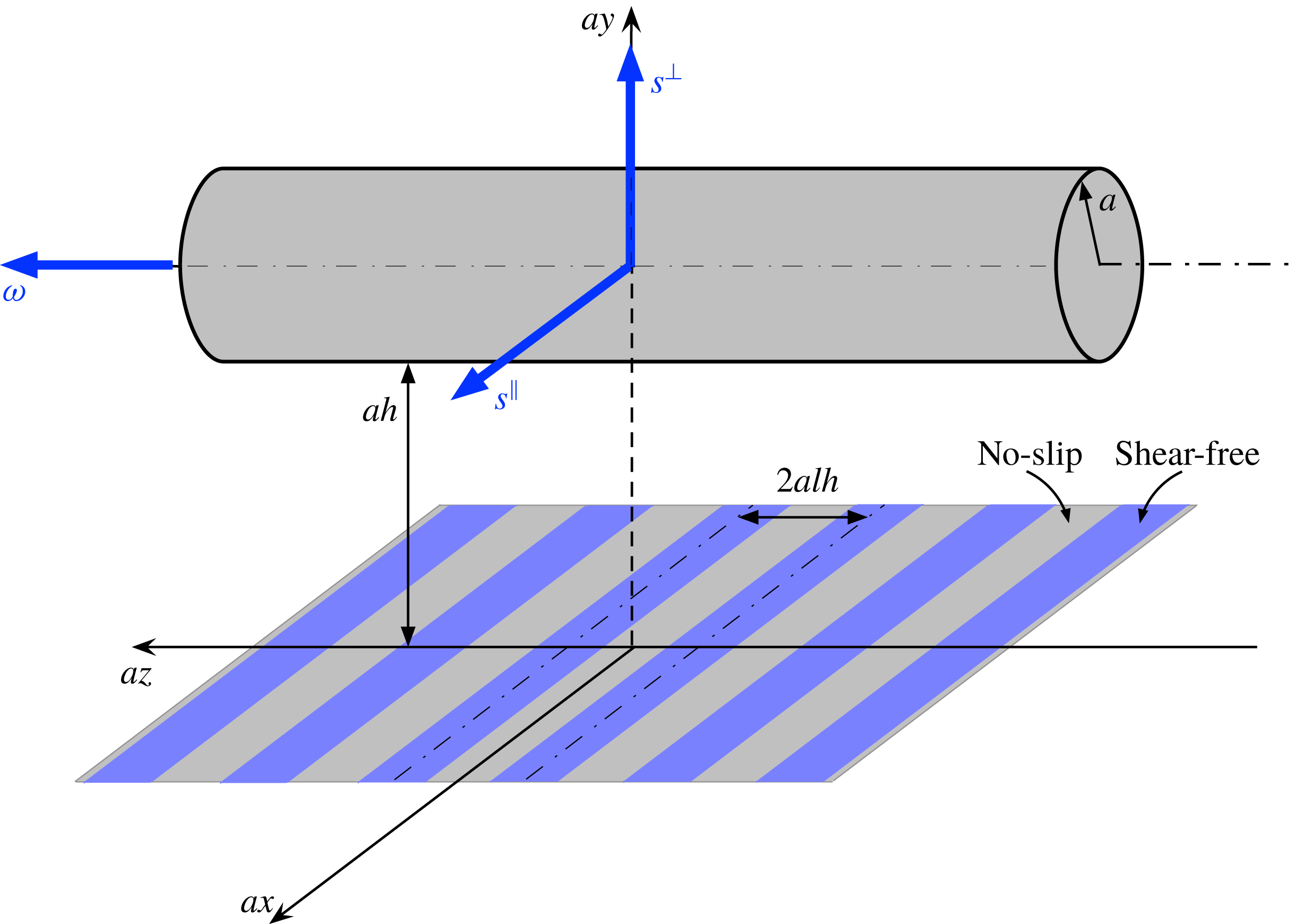
Figure 1. Schematic of the dimensional geometry.
The flow problem we address herein is animated by the composition of three independent modes of rigid-body motion, consisting of: (i) pure translation of the cylinder in the
 $y$
-direction, perpendicular to the surface, with speed
$y$
-direction, perpendicular to the surface, with speed
 $s_{\bot }$
; (ii) pure translation of the cylinder parallel to the surface, in the
$s_{\bot }$
; (ii) pure translation of the cylinder parallel to the surface, in the
 $x$
-direction, at speed
$x$
-direction, at speed
 $s_{\Vert }$
; and (iii) pure rotation of the cylinder about its axis, in the
$s_{\Vert }$
; and (iii) pure rotation of the cylinder about its axis, in the
 $z$
-direction, at angular velocity
$z$
-direction, at angular velocity
 $\unicode[STIX]{x1D714}$
. Assuming from the outset that inertial forces are negligible, the flow equations are quasi-steady. Assuming further that the capillary number is small, the menisci deformation and dilation due to the flow are negligible, and the postulation of a flat interface remains intact. The liquid domain is therefore bounded by the cylinder and the superhydrophobic plane, on which a no-slip condition applies at the solid strips and a shear-free condition at the gaseous strips.
$\unicode[STIX]{x1D714}$
. Assuming from the outset that inertial forces are negligible, the flow equations are quasi-steady. Assuming further that the capillary number is small, the menisci deformation and dilation due to the flow are negligible, and the postulation of a flat interface remains intact. The liquid domain is therefore bounded by the cylinder and the superhydrophobic plane, on which a no-slip condition applies at the solid strips and a shear-free condition at the gaseous strips.
Our interest is in the hydrodynamic forces and torques acting on a unit length of the cylinder, averaged over a single period of the superhydrophobic surface. The symmetry properties of Stokes flow imply (see appendix A) that the force in the
 $y$
-direction possesses the form
$y$
-direction possesses the form
 $$\begin{eqnarray}-\unicode[STIX]{x1D707}\,f^{\bot }s^{\bot },\end{eqnarray}$$
while the force in the
 $x$
-direction and the torque in the
$x$
-direction and the torque in the
 $z$
-direction possess the respective forms
$z$
-direction possess the respective forms
 $$\begin{eqnarray}-\unicode[STIX]{x1D707}(f^{\Vert }s^{\Vert }+ac\unicode[STIX]{x1D714}),\quad -\unicode[STIX]{x1D707}a(cs^{\Vert }+at\unicode[STIX]{x1D714}).\end{eqnarray}$$
Following the introduction of
 $a$
into relations (2.1) and (2.2), the resistance coefficients
$a$
into relations (2.1) and (2.2), the resistance coefficients
 $f^{\bot }$
,
$f^{\bot }$
,
 $f^{\Vert }$
,
$f^{\Vert }$
,
 $c$
and
$c$
and
 $t$
appearing therein are all rendered dimensionless. Note that the same coupling coefficient
$t$
appearing therein are all rendered dimensionless. Note that the same coupling coefficient
 $c$
appears in both the expression for the force due to rotation and that for torque due to translation; in appendix A we show that this reciprocity, which is known to hold for a solid particle that moves through an unbounded fluid domain, also applies in the present configuration, which involves an adjacent planar boundary on which mixed boundary conditions are prescribed.
$c$
appears in both the expression for the force due to rotation and that for torque due to translation; in appendix A we show that this reciprocity, which is known to hold for a solid particle that moves through an unbounded fluid domain, also applies in the present configuration, which involves an adjacent planar boundary on which mixed boundary conditions are prescribed.
We hereafter normalise length variables by
 $a$
. In this notation, the (instantaneous) cylinder–surface clearance is
$a$
. In this notation, the (instantaneous) cylinder–surface clearance is
 $h$
and the grooved-array period is
$h$
and the grooved-array period is
 $2hl$
. The problem periodicity allows one to consider the flow in a single ‘cell’ of lateral extent
$2hl$
. The problem periodicity allows one to consider the flow in a single ‘cell’ of lateral extent
 $2lh$
, say that bounded between
$2lh$
, say that bounded between
 $z=\pm lh$
. Figure 2 depicts the ‘top’ and ‘side’ views of the dimensionless geometry. To determine the resistance coefficients, it is convenient to exploit the Stokes-flow linearity and decompose the flow problem into three subproblems which respectively correspond to perpendicular translation, parallel translation and rotation. Furthermore, we adopt a unified dimensionless notation which applies to all three problems, where velocity variables are normalised by
$z=\pm lh$
. Figure 2 depicts the ‘top’ and ‘side’ views of the dimensionless geometry. To determine the resistance coefficients, it is convenient to exploit the Stokes-flow linearity and decompose the flow problem into three subproblems which respectively correspond to perpendicular translation, parallel translation and rotation. Furthermore, we adopt a unified dimensionless notation which applies to all three problems, where velocity variables are normalised by
 $s$
, the latter being chosen as
$s$
, the latter being chosen as
 $$\begin{eqnarray}s=\left\{\begin{array}{@{}ll@{}}s^{\bot }h^{-1/2}\quad & \text{in the perpendicular-translation problem,}\\ s^{\Vert }\quad & \text{in the parallel-translation problem,}\\ \unicode[STIX]{x1D714}a\quad & \text{in the rotation problem.}\end{array}\right.\end{eqnarray}$$
(Note that all these choices represent a characteristic velocity in the
 $x$
-direction.) Stress variables are normalised by
$x$
-direction.) Stress variables are normalised by
 $\unicode[STIX]{x1D707}s/a$
.
$\unicode[STIX]{x1D707}s/a$
.
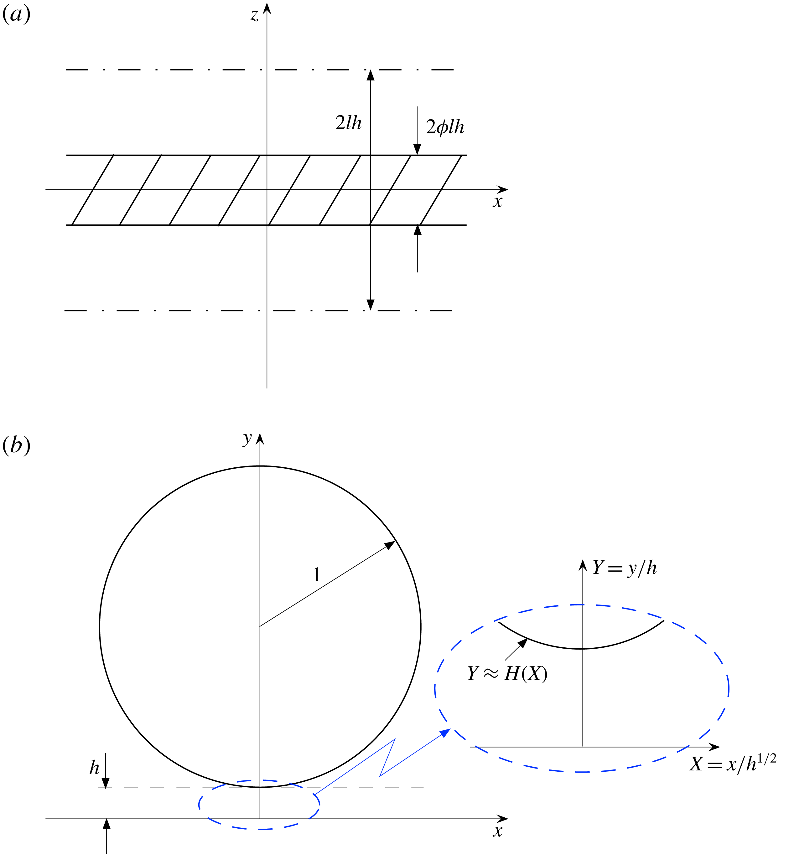
Figure 2. Dimensionless geometry. (a) Top view, showing a single period of the superhydrophobic surface. (b) Side view, with the inset zooming on the gap region.
In our unified description, the governing differential equations and the majority of the supplementary conditions are identical in all three problems. Thus, the differential equations governing the velocity
 $\boldsymbol{u}=\hat{\boldsymbol{e}}_{x}u(x,y,z)+\hat{\boldsymbol{e}}_{y}v(x,y,z)+\hat{\boldsymbol{e}}_{z}w(x,y,z)$
and pressure
$\boldsymbol{u}=\hat{\boldsymbol{e}}_{x}u(x,y,z)+\hat{\boldsymbol{e}}_{y}v(x,y,z)+\hat{\boldsymbol{e}}_{z}w(x,y,z)$
and pressure
 $p(x,y,z)$
consist of the continuity equation,
$p(x,y,z)$
consist of the continuity equation,
 $$\begin{eqnarray}\frac{\unicode[STIX]{x2202}u}{\unicode[STIX]{x2202}x}+\frac{\unicode[STIX]{x2202}v}{\unicode[STIX]{x2202}y}+\frac{\unicode[STIX]{x2202}w}{\unicode[STIX]{x2202}z}=0,\end{eqnarray}$$
and the Stokes equations,
 $$\begin{eqnarray}\frac{\unicode[STIX]{x2202}p}{\unicode[STIX]{x2202}x}=\unicode[STIX]{x1D6FB}^{2}u,\quad \frac{\unicode[STIX]{x2202}p}{\unicode[STIX]{x2202}y}=\unicode[STIX]{x1D6FB}^{2}v,\quad \frac{\unicode[STIX]{x2202}p}{\unicode[STIX]{x2202}z}=\unicode[STIX]{x1D6FB}^{2}w.\end{eqnarray}$$
The boundary conditions at the patterned surface
 $y=0$
consist of impermeability,
$y=0$
consist of impermeability,
 $$\begin{eqnarray}v=0,\end{eqnarray}$$
a no-slip condition at the solid patches,
 $$\begin{eqnarray}u=w=0\quad \text{for }|z|\leqslant \unicode[STIX]{x1D719}lh,\end{eqnarray}$$
and a shear-free condition at the menisci,
 $$\begin{eqnarray}\frac{\unicode[STIX]{x2202}u}{\unicode[STIX]{x2202}y}=\frac{\unicode[STIX]{x2202}w}{\unicode[STIX]{x2202}y}=0\quad \text{for }\unicode[STIX]{x1D719}lh<|z|<lh.\end{eqnarray}$$
In addition, the flow must be
 $2hl$
-periodic in the
$2hl$
-periodic in the
 $z$
-direction and satisfy the requirement that
$z$
-direction and satisfy the requirement that
 $\boldsymbol{u}$
attenuates at large distances from the cylinder. Because of symmetry about
$\boldsymbol{u}$
attenuates at large distances from the cylinder. Because of symmetry about
 $z=0$
, the periodicity conditions may be written as
$z=0$
, the periodicity conditions may be written as
 $$\begin{eqnarray}w=\frac{\unicode[STIX]{x2202}u}{\unicode[STIX]{x2202}z}=\frac{\unicode[STIX]{x2202}v}{\unicode[STIX]{x2202}z}=0\quad \text{at }z=\pm lh.\end{eqnarray}$$
The no-slip conditions on the cylinder boundary depend on the specific problem considered. Thus, in the separate subproblems of perpendicular translation, parallel translation and rotation, we respectively have
 $$\begin{eqnarray}\displaystyle & \displaystyle u=0,\quad v=h^{1/2},\quad w=0, & \displaystyle\end{eqnarray}$$
 $$\begin{eqnarray}\displaystyle & \displaystyle u=1,\quad v=0,\quad w=0, & \displaystyle\end{eqnarray}$$
 $$\begin{eqnarray}\displaystyle & \displaystyle u=1-y+h,\quad v=x,\quad w=0. & \displaystyle\end{eqnarray}$$
Note that the boundary conditions governing
 $w$
are all homogeneous, suggesting that
$w$
are all homogeneous, suggesting that
 $w$
trivially vanishes. The instantaneous velocity field is therefore assumed to be of the quasi-longitudinal form
$w$
trivially vanishes. The instantaneous velocity field is therefore assumed to be of the quasi-longitudinal form
 $\boldsymbol{u}=\hat{\boldsymbol{e}}_{x}u(x,y,z)+\hat{\boldsymbol{e}}_{y}v(x,y,z)$
. It then follows from (2.5b
) that the pressure
$\boldsymbol{u}=\hat{\boldsymbol{e}}_{x}u(x,y,z)+\hat{\boldsymbol{e}}_{y}v(x,y,z)$
. It then follows from (2.5b
) that the pressure
 $p$
is independent of
$p$
is independent of
 $z$
, say
$z$
, say
 $p(x,y)$
. Because of symmetry about
$p(x,y)$
. Because of symmetry about
 $z=0$
, we can further reduce the pertinent domain to the half-period
$z=0$
, we can further reduce the pertinent domain to the half-period
 $0<z<lh$
with (2.9) applying at
$0<z<lh$
with (2.9) applying at
 $z=0$
and
$z=0$
and
 $z=lh$
. The other obvious symmetry about
$z=lh$
. The other obvious symmetry about
 $x=0$
implies that, in the case of perpendicular translation,
$x=0$
implies that, in the case of perpendicular translation,
 $p$
and
$p$
and
 $v$
are even functions of
$v$
are even functions of
 $x$
while
$x$
while
 $u$
is an odd function of it. In the cases of parallel translation and rotation, the opposite holds.
$u$
is an odd function of it. In the cases of parallel translation and rotation, the opposite holds.
3 Near-contact limit
3.1 Gap coordinates and scalings
Our interest is in the limit
 $h\rightarrow 0$
with
$h\rightarrow 0$
with
 $l=O(1)$
, namely where the cylinder–surface clearance is comparable to the microstructure periodicity, and both are small compared to the cylinder radius. The limit
$l=O(1)$
, namely where the cylinder–surface clearance is comparable to the microstructure periodicity, and both are small compared to the cylinder radius. The limit
 $h\rightarrow 0$
is naturally accommodated by zooming in the gap using the stretched coordinates
$h\rightarrow 0$
is naturally accommodated by zooming in the gap using the stretched coordinates
 $$\begin{eqnarray}X=x/h^{1/2},\quad Y=y/h,\quad Z=z/h.\end{eqnarray}$$
In terms of these gap-scale coordinates, the cylinder surface becomes
 $Y=H(X)+O(h)$
, where
$Y=H(X)+O(h)$
, where
 $H=1+X^{2}/2$
. The unit vector normal to the cylinder (pointing into the liquid domain) is
$H=1+X^{2}/2$
. The unit vector normal to the cylinder (pointing into the liquid domain) is
 $$\begin{eqnarray}\hat{\boldsymbol{n}}\sim -(\hat{\boldsymbol{e}}_{y}-h^{1/2}X\hat{\boldsymbol{e}}_{x})[1+O(h)].\end{eqnarray}$$
With the choice (2.3) of the velocity scale
 $s$
in the three subproblems, the near-contact scalings of the pressure and two velocity components are identical in all three problems,
$s$
in the three subproblems, the near-contact scalings of the pressure and two velocity components are identical in all three problems,
 $$\begin{eqnarray}p=O(h^{-3/2}),\quad u=O(1),\quad v=O(h^{1/2}),\end{eqnarray}$$
thus allowing for a truly unified analysis (as in Kaynan & Yariv Reference Kaynan and Yariv2017). We therefore employ the following asymptotic expansions of the flow variables:
 $$\begin{eqnarray}p=h^{-3/2}P(X,Y)+\cdots \,,\quad u=U(X,Y,Z)+\cdots \,,\quad v=h^{1/2}V(X,Y,Z)+\cdots \,,\end{eqnarray}$$
where
 $P$
,
$P$
,
 $U$
and
$U$
and
 $V$
are
$V$
are
 $O(1)$
.
$O(1)$
.
3.2 Leading-order problem
The leading-order inner variables satisfy the following:
(i) the continuity equation,
(3.5) $$\begin{eqnarray}\frac{\unicode[STIX]{x2202}U}{\unicode[STIX]{x2202}X}+\frac{\unicode[STIX]{x2202}V}{\unicode[STIX]{x2202}Y}=0;\end{eqnarray}$$
(ii) the momentum balances,
(3.6a,b )$$\begin{eqnarray}\frac{\unicode[STIX]{x2202}P}{\unicode[STIX]{x2202}X}=\frac{\unicode[STIX]{x2202}^{2}U}{\unicode[STIX]{x2202}Y^{2}}+\frac{\unicode[STIX]{x2202}^{2}U}{\unicode[STIX]{x2202}Z^{2}},\quad \frac{\unicode[STIX]{x2202}P}{\unicode[STIX]{x2202}Y}=0;\end{eqnarray}$$
(iii) conditions at the compound surface
$Y=0$
, consisting of impermeability, (3.7)no slip at the solid strip,$$\begin{eqnarray}V=0,\end{eqnarray}$$
(3.8)and no shear at the free surface,$$\begin{eqnarray}U=0\quad \text{for }0<Z<\unicode[STIX]{x1D719}l,\end{eqnarray}$$
(3.9)$$\begin{eqnarray}\frac{\unicode[STIX]{x2202}U}{\unicode[STIX]{x2202}Y}=0\quad \text{for }\unicode[STIX]{x1D719}l<Z<l;\end{eqnarray}$$
(iv) the symmetry and periodicity conditions,
(3.10)$$\begin{eqnarray}\frac{\unicode[STIX]{x2202}U}{\unicode[STIX]{x2202}Z}=\frac{\unicode[STIX]{x2202}V}{\unicode[STIX]{x2202}Z}=0\quad \text{at }Z=0,l;\end{eqnarray}$$


and (v) the no-slip conditions at
 $Y=H(X)$
(cf. (2.10)),
$Y=H(X)$
(cf. (2.10)),
 $$\begin{eqnarray}\displaystyle U=0,\quad & V=1 & \displaystyle \quad \text{in the perpendicular-translation problem},\end{eqnarray}$$
 $$\begin{eqnarray}\displaystyle U=1,\quad & V=0 & \displaystyle \quad \text{in the parallel-translation problem},\end{eqnarray}$$
 $$\begin{eqnarray}\displaystyle U=1,\quad & V=X & \displaystyle \quad \text{in the rotation problem}.\end{eqnarray}$$
The far-field velocity decay does not apply in the gap region; it is replaced by the requirement of asymptotic matching with the ‘outer’ solution outside the gap. In particular, given the
 $O(1)$
pressure scaling there,
$O(1)$
pressure scaling there,
 $$\begin{eqnarray}\lim _{X\rightarrow \pm \infty }P=0.\end{eqnarray}$$
Finally, we note that the pressure scaling (3.3a
) in conjunction with the
 $O(h^{1/2})$
extent of the gap in the
$O(h^{1/2})$
extent of the gap in the
 $x$
-direction implies an
$x$
-direction implies an
 $O(h^{-3/2})$
gap-scale contribution to
$O(h^{-3/2})$
gap-scale contribution to
 $f^{\bot }$
. Similarly, the velocity scaling (3.3b
) in conjunction with the
$f^{\bot }$
. Similarly, the velocity scaling (3.3b
) in conjunction with the
 $O(h)$
extent of the gap in the
$O(h)$
extent of the gap in the
 $y$
-direction implies that, within the gap, the shear stresses in the
$y$
-direction implies that, within the gap, the shear stresses in the
 $xy$
-plane are
$xy$
-plane are
 $O(h^{-1})$
; their contributions to
$O(h^{-1})$
; their contributions to
 $f^{\Vert }$
,
$f^{\Vert }$
,
 $c$
and
$c$
and
 $t$
are accordingly
$t$
are accordingly
 $O(h^{-1/2})$
. Since the outer contributions to the hydrodynamic loads from the region outside the gap are clearly
$O(h^{-1/2})$
. Since the outer contributions to the hydrodynamic loads from the region outside the gap are clearly
 $O(1)$
, and hence subdominant, we conclude that
$O(1)$
, and hence subdominant, we conclude that
 $$\begin{eqnarray}f^{\bot }=h^{-3/2}F^{\bot }+\cdots\end{eqnarray}$$
and
 $$\begin{eqnarray}f^{\Vert }=h^{-1/2}F^{\Vert }+\cdots \,,\quad c=h^{-1/2}C+\cdots \,,\quad t=h^{-1/2}T+\cdots \,,\end{eqnarray}$$
where the
 $O(1)$
coefficients
$O(1)$
coefficients
 $F^{\bot }$
,
$F^{\bot }$
,
 $F^{\Vert }$
,
$F^{\Vert }$
,
 $C$
and
$C$
and
 $T$
are unaffected by the outer region. As these coefficients are independent of
$T$
are unaffected by the outer region. As these coefficients are independent of
 $h$
, they depend only upon the geometric parameters
$h$
, they depend only upon the geometric parameters
 $l$
and
$l$
and
 $\unicode[STIX]{x1D719}$
.
$\unicode[STIX]{x1D719}$
.
An ad hoc procedure which allows for the preceding coefficient to be readily calculated involves replacement of the mixed conditions at the compound surface by a presumably equivalent Navier-slip condition. This procedure, which provides useful approximations for small
 $l$
, is described in appendix B. In what follows, we proceed with a systematic analysis of the longitudinal flow in the inner region.
$l$
, is described in appendix B. In what follows, we proceed with a systematic analysis of the longitudinal flow in the inner region.
4 Two cell problems
4.1 Decomposition of the longitudinal flow
From (3.6b
) we find that
 $P$
is also independent of
$P$
is also independent of
 $Y$
, say
$Y$
, say
 $P(X)$
. The problem governing
$P(X)$
. The problem governing
 $U$
is therefore uncoupled to that governing
$U$
is therefore uncoupled to that governing
 $V$
. It consists of the Poisson equation (cf. (3.6a
))
$V$
. It consists of the Poisson equation (cf. (3.6a
))
 $$\begin{eqnarray}\frac{\unicode[STIX]{x2202}^{2}U}{\unicode[STIX]{x2202}Y^{2}}+\frac{\unicode[STIX]{x2202}^{2}U}{\unicode[STIX]{x2202}Z^{2}}=\frac{\text{d}P}{\text{d}X},\end{eqnarray}$$
together with the conditions governing
 $U$
, consisting of (3.8)–(3.10) and either one of (3.11) on the cylinder boundary.
$U$
, consisting of (3.8)–(3.10) and either one of (3.11) on the cylinder boundary.
Consider first the case of perpendicular translation, where the boundary condition governing
 $U$
on the cylinder is homogeneous, see (3.11a
). It then follows that all the pertinent boundary conditions are homogeneous, implying that the problem governing
$U$
on the cylinder is homogeneous, see (3.11a
). It then follows that all the pertinent boundary conditions are homogeneous, implying that the problem governing
 $U$
is forced solely by the pressure gradient
$U$
is forced solely by the pressure gradient
 $\text{d}P/\text{d}X$
. From (4.1) we then find that
$\text{d}P/\text{d}X$
. From (4.1) we then find that
 $U$
must be linear in
$U$
must be linear in
 $\text{d}P/\text{d}X$
. Moreover, after factoring out
$\text{d}P/\text{d}X$
. Moreover, after factoring out
 $\text{d}P/\text{d}X$
, the dependence upon
$\text{d}P/\text{d}X$
, the dependence upon
 $X$
enters only through the application of boundary conditions at
$X$
enters only through the application of boundary conditions at
 $Y=H(X)$
. It therefore follows that
$Y=H(X)$
. It therefore follows that
 $U$
may be represented in terms of an
$U$
may be represented in terms of an
 $X$
-independent ‘pressure-driven’ cell function
$X$
-independent ‘pressure-driven’ cell function
 ${\mathcal{U}}_{P}(Y,Z;{\mathcal{H}})$
via the relation
${\mathcal{U}}_{P}(Y,Z;{\mathcal{H}})$
via the relation
 $$\begin{eqnarray}U(X,Y,Z)=-\frac{\text{d}P}{\text{d}X}\,{\mathcal{U}}_{P}(Y,Z;H(X)).\end{eqnarray}$$
In the cases of parallel translation and rotation, the problem governing
 $U$
is further forced by an (identical) inhomogeneous boundary condition satisfied by
$U$
is further forced by an (identical) inhomogeneous boundary condition satisfied by
 $U$
at
$U$
at
 $Y=H(X)$
. For these problems,
$Y=H(X)$
. For these problems,
 $$\begin{eqnarray}U(X,Y,Z)=-\frac{\text{d}P}{\text{d}X}\,{\mathcal{U}}_{P}(Y,Z;H(X))+{\mathcal{U}}_{B}(Y,Z;H(X)),\end{eqnarray}$$
where we introduce a ‘boundary-driven’ cell function
 ${\mathcal{U}}_{B}(Y,Z;{\mathcal{H}})$
. (The distributions of
${\mathcal{U}}_{B}(Y,Z;{\mathcal{H}})$
. (The distributions of
 $P(X)$
in these two cases are obviously different.) We next discuss the pressure-driven and boundary-driven cell problems governing
$P(X)$
in these two cases are obviously different.) We next discuss the pressure-driven and boundary-driven cell problems governing
 ${\mathcal{U}}_{P}$
and
${\mathcal{U}}_{P}$
and
 ${\mathcal{U}}_{B}$
, respectively.
${\mathcal{U}}_{B}$
, respectively.
4.2 Pressure-driven cell problem
The cell problem governing
 ${\mathcal{U}}_{P}(Y,Z;{\mathcal{H}})$
consists of the following:
${\mathcal{U}}_{P}(Y,Z;{\mathcal{H}})$
consists of the following:
(i) Poisson’s equation,
(4.4)$$\begin{eqnarray}\frac{\unicode[STIX]{x2202}^{2}{\mathcal{U}}_{P}}{\unicode[STIX]{x2202}Y^{2}}+\frac{\unicode[STIX]{x2202}^{2}{\mathcal{U}}_{P}}{\unicode[STIX]{x2202}Z^{2}}=-1\quad \text{for }0<Z<l,~0<Y<{\mathcal{H}};\end{eqnarray}$$
(ii) no slip at the top boundary,
(4.5)$$\begin{eqnarray}{\mathcal{U}}_{P}=0\quad \text{at }Y={\mathcal{H}};\end{eqnarray}$$
(iii) the mixed conditions at
$Y=0$
, (4.6a,b )$$\begin{eqnarray}{\mathcal{U}}_{P}=0\quad \text{for }0<Z<\unicode[STIX]{x1D719}l,\quad \frac{\unicode[STIX]{x2202}{\mathcal{U}}_{P}}{\unicode[STIX]{x2202}Y}=0\quad \text{for }\unicode[STIX]{x1D719}l<Z<l;\end{eqnarray}$$


and (iv) the symmetry conditions,
 $$\begin{eqnarray}\frac{\unicode[STIX]{x2202}{\mathcal{U}}_{P}}{\unicode[STIX]{x2202}Z}=0\quad \text{at }Z=0,l.\end{eqnarray}$$
In addition to
 ${\mathcal{H}}$
,
${\mathcal{H}}$
,
 ${\mathcal{U}}_{P}$
also depends upon the texture parameters
${\mathcal{U}}_{P}$
also depends upon the texture parameters
 $l$
and
$l$
and
 $\unicode[STIX]{x1D719}$
. As a consequence, all integral properties of the cell problem are functions of
$\unicode[STIX]{x1D719}$
. As a consequence, all integral properties of the cell problem are functions of
 ${\mathcal{H}}$
,
${\mathcal{H}}$
,
 $l$
and
$l$
and
 $\unicode[STIX]{x1D719}$
. Two of these properties play a key role in the following analysis. The first is the averaged cross-sectional volumetric flux,
$\unicode[STIX]{x1D719}$
. Two of these properties play a key role in the following analysis. The first is the averaged cross-sectional volumetric flux,
 $$\begin{eqnarray}{\mathcal{Q}}_{P}({\mathcal{H}},l,\unicode[STIX]{x1D719})=l^{-1}\int _{0}^{l}\text{d}Z\int _{0}^{{\mathcal{H}}}\text{d}Y\;{\mathcal{U}}_{P}(Y,Z;{\mathcal{H}}).\end{eqnarray}$$
The second is the averaged shear stress at the top boundary (in the negative
 $x$
-direction)
$x$
-direction)
 $$\begin{eqnarray}{\mathcal{S}}_{P}({\mathcal{H}},l,\unicode[STIX]{x1D719})=l^{-1}\int _{0}^{l}\text{d}Z\left[\frac{\unicode[STIX]{x2202}}{\unicode[STIX]{x2202}Y}\,{\mathcal{U}}_{P}(Y,Z;{\mathcal{H}})\right]_{Y={\mathcal{H}}}.\end{eqnarray}$$
Consider now
 $l$
and
$l$
and
 $\unicode[STIX]{x1D719}$
as fixed, whereby
$\unicode[STIX]{x1D719}$
as fixed, whereby
 ${\mathcal{U}}_{P}$
depends upon the single parameter
${\mathcal{U}}_{P}$
depends upon the single parameter
 ${\mathcal{H}}$
and is written as
${\mathcal{H}}$
and is written as
 ${\mathcal{U}}_{P}(Y,Z;{\mathcal{H}})$
. It is easy to verify by a rescaling of the cell problem that
${\mathcal{U}}_{P}(Y,Z;{\mathcal{H}})$
. It is easy to verify by a rescaling of the cell problem that
 ${\mathcal{U}}_{P}(Y,Z;{\mathcal{H}})$
is a homogeneous function of degree two in its three arguments, namely
${\mathcal{U}}_{P}(Y,Z;{\mathcal{H}})$
is a homogeneous function of degree two in its three arguments, namely
 $$\begin{eqnarray}{\mathcal{U}}_{P}(Y,Z;{\mathcal{H}})={\mathcal{H}}^{2}\,{\mathcal{U}}_{P}(Y/{\mathcal{H}},Z/{\mathcal{H}};1).\end{eqnarray}$$
The integral volume flux and average shear stress thus transform as
 $$\begin{eqnarray}{\mathcal{Q}}_{P}({\mathcal{H}},l,\unicode[STIX]{x1D719})={\mathcal{H}}^{3}{\mathcal{Q}}_{P}(1,l/{\mathcal{H}},\unicode[STIX]{x1D719}),\quad {\mathcal{S}}_{P}({\mathcal{H}},l,\unicode[STIX]{x1D719})={\mathcal{H}}{\mathcal{S}}_{P}(1,l/{\mathcal{H}},\unicode[STIX]{x1D719}).\end{eqnarray}$$
These transformations accordingly allow one to relate the integral properties of the original cell to those corresponding to a unit-depth cell (denoted hereafter the ‘standard cell’). These relations, in turn, reduce the number of geometric parameters by one when seeking to determine the complete dependence of
 ${\mathcal{Q}}_{P}$
and
${\mathcal{Q}}_{P}$
and
 ${\mathcal{S}}_{P}$
upon the cell geometry.
${\mathcal{S}}_{P}$
upon the cell geometry.
It is accordingly beneficial to define the standard-cell velocity field
 $$\begin{eqnarray}\tilde{{\mathcal{U}}}_{P}(Y,Z)\stackrel{\text{def}}{=}{\mathcal{U}}_{P}(Y,Z;1)\end{eqnarray}$$
and the associated integral quantities
 $$\begin{eqnarray}\tilde{{\mathcal{Q}}}_{P}(l,\unicode[STIX]{x1D719})\stackrel{\text{def}}{=}{\mathcal{Q}}_{P}(1,l,\unicode[STIX]{x1D719}),\quad \tilde{{\mathcal{S}}}_{P}(l,\unicode[STIX]{x1D719})\stackrel{\text{def}}{=}{\mathcal{S}}_{P}(1,l,\unicode[STIX]{x1D719}).\end{eqnarray}$$
The latter are related to the standard-cell velocity field via the relations (cf. (4.8) and (4.9))
 $$\begin{eqnarray}\tilde{{\mathcal{Q}}}_{P}=l^{-1}\int _{0}^{l}\text{d}Z\int _{0}^{1}\text{d}Y\;\tilde{{\mathcal{U}}}_{P}(Y,Z),\quad \tilde{{\mathcal{S}}}_{P}=l^{-1}\int _{0}^{l}\text{d}Z\left.\frac{\unicode[STIX]{x2202}\tilde{{\mathcal{U}}}_{P}}{\unicode[STIX]{x2202}Y}\right|_{Y=1}.\end{eqnarray}$$
Transformations (4.11) thus read
 $$\begin{eqnarray}{\mathcal{Q}}_{P}({\mathcal{H}},l,\unicode[STIX]{x1D719})={\mathcal{H}}^{3}\tilde{{\mathcal{Q}}}_{P}(l/{\mathcal{H}},\unicode[STIX]{x1D719}),\quad {\mathcal{S}}_{P}({\mathcal{H}},l,\unicode[STIX]{x1D719})={\mathcal{H}}\tilde{{\mathcal{S}}}_{P}(l/{\mathcal{H}},\unicode[STIX]{x1D719}).\end{eqnarray}$$
4.3 Boundary-driven cell problem
Consider now the cell problem governing
 ${\mathcal{U}}_{B}(Y,Z;{\mathcal{H}})$
. It consists of Laplace’s equation,
${\mathcal{U}}_{B}(Y,Z;{\mathcal{H}})$
. It consists of Laplace’s equation,
 $$\begin{eqnarray}\frac{\unicode[STIX]{x2202}^{2}{\mathcal{U}}_{B}}{\unicode[STIX]{x2202}Y^{2}}+\frac{\unicode[STIX]{x2202}^{2}{\mathcal{U}}_{B}}{\unicode[STIX]{x2202}Z^{2}}=0\quad \text{for }0<Z<l,~0<Y<{\mathcal{H}},\end{eqnarray}$$
and is forced by an inhomogeneous condition at the top boundary,
 $$\begin{eqnarray}{\mathcal{U}}_{B}=1\quad \text{at }Y={\mathcal{H}}.\end{eqnarray}$$
Otherwise, it satisfies the same mixed conditions at
 $Y=0$
and symmetry conditions that appear in the pressure-driven cell problem. The integral quantities
$Y=0$
and symmetry conditions that appear in the pressure-driven cell problem. The integral quantities
 ${\mathcal{Q}}_{B}({\mathcal{H}},l,\unicode[STIX]{x1D719})$
and
${\mathcal{Q}}_{B}({\mathcal{H}},l,\unicode[STIX]{x1D719})$
and
 ${\mathcal{S}}_{B}({\mathcal{H}},l,\unicode[STIX]{x1D719})$
are defined in a manner similar to (4.8) and (4.9), with
${\mathcal{S}}_{B}({\mathcal{H}},l,\unicode[STIX]{x1D719})$
are defined in a manner similar to (4.8) and (4.9), with
 ${\mathcal{U}}_{B}$
used instead of
${\mathcal{U}}_{B}$
used instead of
 ${\mathcal{U}}_{P}$
.
${\mathcal{U}}_{P}$
.
Consider now
 $l$
and
$l$
and
 $\unicode[STIX]{x1D719}$
as fixed, whereby
$\unicode[STIX]{x1D719}$
as fixed, whereby
 ${\mathcal{U}}_{B}$
depends upon the single parameter
${\mathcal{U}}_{B}$
depends upon the single parameter
 ${\mathcal{H}}$
and is written as
${\mathcal{H}}$
and is written as
 ${\mathcal{U}}_{B}(Y,Z;{\mathcal{H}})$
. It is easy to verify that
${\mathcal{U}}_{B}(Y,Z;{\mathcal{H}})$
. It is easy to verify that
 ${\mathcal{U}}_{B}(Y,Z;{\mathcal{H}})$
is a homogeneous function of zeroth degree in its three arguments:
${\mathcal{U}}_{B}(Y,Z;{\mathcal{H}})$
is a homogeneous function of zeroth degree in its three arguments:
 $$\begin{eqnarray}{\mathcal{U}}_{B}(Y,Z;{\mathcal{H}})={\mathcal{U}}_{B}(Y/{\mathcal{H}},Z/{\mathcal{H}};1).\end{eqnarray}$$
The integral volume flux and average shear stress thus transform as
 $$\begin{eqnarray}{\mathcal{Q}}_{B}({\mathcal{H}},l,\unicode[STIX]{x1D719})={\mathcal{H}}{\mathcal{Q}}_{B}(1,l/{\mathcal{H}},\unicode[STIX]{x1D719}),\quad {\mathcal{S}}_{B}({\mathcal{H}},l,\unicode[STIX]{x1D719})={\mathcal{H}}^{-1}{\mathcal{S}}_{B}(1,l/{\mathcal{H}},\unicode[STIX]{x1D719}).\end{eqnarray}$$
As in the pressure-driven cell problem, we define the standard-cell velocity field,
 $$\begin{eqnarray}\tilde{{\mathcal{U}}}_{B}(Y,Z)\stackrel{\text{def}}{=}{\mathcal{U}}_{B},(Y,Z;1),\end{eqnarray}$$
and the associated cell flux and mean shear,
 $$\begin{eqnarray}\tilde{{\mathcal{Q}}}_{B}(l,\unicode[STIX]{x1D719})\stackrel{\text{def}}{=}{\mathcal{Q}}_{B}(1,l,\unicode[STIX]{x1D719}),\quad \tilde{{\mathcal{S}}}_{B}(l,\unicode[STIX]{x1D719})\stackrel{\text{def}}{=}{\mathcal{S}}_{B}(1,l,\unicode[STIX]{x1D719}).\end{eqnarray}$$
These integral quantities are provided by
 $$\begin{eqnarray}\tilde{{\mathcal{Q}}}_{B}=l^{-1}\int _{0}^{l}\text{d}Z\int _{0}^{1}\text{d}Y\;\tilde{{\mathcal{U}}}_{B}(Y,Z),\quad \tilde{{\mathcal{S}}}_{B}=l^{-1}\int _{0}^{l}\text{d}Z\left.\frac{\unicode[STIX]{x2202}\tilde{{\mathcal{U}}}_{B}}{\unicode[STIX]{x2202}Y}\right|_{Y=1}.\end{eqnarray}$$
Transformations (4.19) thus read
 $$\begin{eqnarray}{\mathcal{Q}}_{B}({\mathcal{H}},l,\unicode[STIX]{x1D719})={\mathcal{H}}\tilde{{\mathcal{Q}}}_{B}(l/{\mathcal{H}},\unicode[STIX]{x1D719}),\quad {\mathcal{S}}_{B}({\mathcal{H}},l,\unicode[STIX]{x1D719})={\mathcal{H}}^{-1}\tilde{{\mathcal{S}}}_{B}(l/{\mathcal{H}},\unicode[STIX]{x1D719}).\end{eqnarray}$$
4.4 Properties of
$\tilde{{\mathcal{Q}}}_{P}$
and
$\tilde{{\mathcal{S}}}_{P}$


The function
 $\tilde{{\mathcal{Q}}}_{P}(l,\unicode[STIX]{x1D719})$
was provided by Philip (Reference Philip1972b
) as the solution of a transcendental equation, itself obtained from the conformal-map calculation of the velocity field (Philip Reference Philip1972a
). Given the complexity of that equation, which involves elliptic integrals, contemporary analyses of the standard-cell geometry (Sbragaglia & Prosperetti Reference Sbragaglia and Prosperetti2007; Teo & Khoo Reference Teo and Khoo2009) typically represent the solution via an appropriate Fourier series and evaluate its coefficients (of which only one affects the value of
$\tilde{{\mathcal{Q}}}_{P}(l,\unicode[STIX]{x1D719})$
was provided by Philip (Reference Philip1972b
) as the solution of a transcendental equation, itself obtained from the conformal-map calculation of the velocity field (Philip Reference Philip1972a
). Given the complexity of that equation, which involves elliptic integrals, contemporary analyses of the standard-cell geometry (Sbragaglia & Prosperetti Reference Sbragaglia and Prosperetti2007; Teo & Khoo Reference Teo and Khoo2009) typically represent the solution via an appropriate Fourier series and evaluate its coefficients (of which only one affects the value of
 $\tilde{{\mathcal{Q}}}_{P}$
) by solving the dual series equations which follow from the mixed boundary conditions at the compound surface (cf. Lauga & Stone Reference Lauga and Stone2003). In what follows, we also need
$\tilde{{\mathcal{Q}}}_{P}$
) by solving the dual series equations which follow from the mixed boundary conditions at the compound surface (cf. Lauga & Stone Reference Lauga and Stone2003). In what follows, we also need
 $\tilde{{\mathcal{S}}}_{P}$
, which to the best of our knowledge has never been calculated.
$\tilde{{\mathcal{S}}}_{P}$
, which to the best of our knowledge has never been calculated.
We accordingly choose here to evaluate the quantities
 $\tilde{{\mathcal{Q}}}_{P}(l,\unicode[STIX]{x1D719})$
and
$\tilde{{\mathcal{Q}}}_{P}(l,\unicode[STIX]{x1D719})$
and
 $\tilde{{\mathcal{S}}}_{P}(l,\unicode[STIX]{x1D719})$
using a Fourier-series representation of the standard-cell field
$\tilde{{\mathcal{S}}}_{P}(l,\unicode[STIX]{x1D719})$
using a Fourier-series representation of the standard-cell field
 $\tilde{{\mathcal{U}}}_{P}$
. The details of the calculation methodology are provided in appendix C. The calculation itself has been performed for several values of
$\tilde{{\mathcal{U}}}_{P}$
. The details of the calculation methodology are provided in appendix C. The calculation itself has been performed for several values of
 $\unicode[STIX]{x1D719}$
(
$\unicode[STIX]{x1D719}$
(
 $0.3$
,
$0.3$
,
 $0.5$
and
$0.5$
and
 $0.7$
); for each of these values,
$0.7$
); for each of these values,
 $\tilde{{\mathcal{Q}}}_{P}$
and
$\tilde{{\mathcal{Q}}}_{P}$
and
 $\tilde{{\mathcal{S}}}_{P}$
have been determined for a large number of
$\tilde{{\mathcal{S}}}_{P}$
have been determined for a large number of
 $l$
-values (ranging from
$l$
-values (ranging from
 $10^{-6}$
to
$10^{-6}$
to
 $10^{6}$
).
$10^{6}$
).
In what follows we provide several asymptotic properties of
 $\tilde{{\mathcal{Q}}}_{P}(l,\unicode[STIX]{x1D719})$
and
$\tilde{{\mathcal{Q}}}_{P}(l,\unicode[STIX]{x1D719})$
and
 $\tilde{{\mathcal{S}}}_{P}(l,\unicode[STIX]{x1D719})$
which may be deduced without referring to the above-mentioned semi-numerical solutions.
$\tilde{{\mathcal{S}}}_{P}(l,\unicode[STIX]{x1D719})$
which may be deduced without referring to the above-mentioned semi-numerical solutions.
4.4.1 Homogeneous solid surface
When
 $\unicode[STIX]{x1D719}=1$
,
$\unicode[STIX]{x1D719}=1$
,
 $\tilde{{\mathcal{U}}}_{P}$
is independent of
$\tilde{{\mathcal{U}}}_{P}$
is independent of
 $Z$
: it is then the familiar Poiseuille flow between two solid walls,
$Z$
: it is then the familiar Poiseuille flow between two solid walls,
 $$\begin{eqnarray}\tilde{{\mathcal{U}}}_{P}=\frac{Y-Y^{2}}{2}.\end{eqnarray}$$
The corresponding volumetric flux and average shear stress are
 $$\begin{eqnarray}\lim _{\unicode[STIX]{x1D719}\rightarrow 1}\tilde{{\mathcal{Q}}}_{P}=\frac{1}{12},\quad \lim _{\unicode[STIX]{x1D719}\rightarrow 1}\tilde{{\mathcal{S}}}_{P}=-\frac{1}{2}.\end{eqnarray}$$
4.4.2 Homogeneous free surface
When
 $\unicode[STIX]{x1D719}=0$
,
$\unicode[STIX]{x1D719}=0$
,
 $\tilde{{\mathcal{U}}}_{P}$
is again independent of
$\tilde{{\mathcal{U}}}_{P}$
is again independent of
 $Z$
: it is now given by the Poiseuille flow between a solid wall and a free surface,
$Z$
: it is now given by the Poiseuille flow between a solid wall and a free surface,
 $$\begin{eqnarray}\tilde{{\mathcal{U}}}_{P}=\frac{1-Y^{2}}{2}.\end{eqnarray}$$
The corresponding volumetric flux is four times as much as before,
 $$\begin{eqnarray}\lim _{\unicode[STIX]{x1D719}\rightarrow 0}\tilde{{\mathcal{Q}}}_{P}=\frac{1}{3}.\end{eqnarray}$$
The average shear stress is
 $$\begin{eqnarray}\lim _{\unicode[STIX]{x1D719}\rightarrow 0}\tilde{{\mathcal{S}}}_{P}=-1.\end{eqnarray}$$
4.4.3 Deep cell
When
 $l\ll 1$
the unit cell appears deep. It follows that the Poiseuille profile (4.24) approximately applies, except in a narrow region several multiples of
$l\ll 1$
the unit cell appears deep. It follows that the Poiseuille profile (4.24) approximately applies, except in a narrow region several multiples of
 $l$
away from the compound surface. At leading order, this accordingly results in the same flux as in the case of a homogeneous solid wall:
$l$
away from the compound surface. At leading order, this accordingly results in the same flux as in the case of a homogeneous solid wall:
 $$\begin{eqnarray}\lim _{l\rightarrow 0}\tilde{{\mathcal{Q}}}_{P}=\frac{1}{12},\quad \lim _{l\rightarrow 0}\tilde{{\mathcal{S}}}_{P}=-\frac{1}{2}.\end{eqnarray}$$
Making use of (4.15), the limit (4.29) readily provides a large-
 $X$
approximation for both
$X$
approximation for both
 ${\mathcal{Q}}_{P}(H(X),l,\unicode[STIX]{x1D719})$
and
${\mathcal{Q}}_{P}(H(X),l,\unicode[STIX]{x1D719})$
and
 ${\mathcal{S}}_{P}(H(X),l,\unicode[STIX]{x1D719})$
. Thus, since
${\mathcal{S}}_{P}(H(X),l,\unicode[STIX]{x1D719})$
. Thus, since
 $H(X)\sim X^{2}/2$
as
$H(X)\sim X^{2}/2$
as
 $X\rightarrow \infty$
, it follows that
$X\rightarrow \infty$
, it follows that
 $$\begin{eqnarray}{\mathcal{Q}}_{P}(H(X),l,\unicode[STIX]{x1D719})\sim \frac{X^{6}}{96}\quad \text{as }X\rightarrow \infty\end{eqnarray}$$
and
 $$\begin{eqnarray}{\mathcal{S}}_{P}(H(X),l,\unicode[STIX]{x1D719})\sim -\frac{X^{2}}{4}\quad \text{as }X\rightarrow \infty .\end{eqnarray}$$
4.4.4 Shallow cell
For
 $l\gg 1$
, where the cell appears shallow, a Hele-Shaw approximation is readily applied, where the velocity profiles (4.24) and (4.26) respectively hold in the intervals
$l\gg 1$
, where the cell appears shallow, a Hele-Shaw approximation is readily applied, where the velocity profiles (4.24) and (4.26) respectively hold in the intervals
 $0<Z<\unicode[STIX]{x1D719}l$
and
$0<Z<\unicode[STIX]{x1D719}l$
and
 $\unicode[STIX]{x1D719}<Z<l$
, with the extent of the transition region connecting these intervals being small compared to
$\unicode[STIX]{x1D719}<Z<l$
, with the extent of the transition region connecting these intervals being small compared to
 $l$
. (A related approximation was used by Feuillebois, Bazant & Vinogradova (Reference Feuillebois, Bazant and Vinogradova2009).) The corresponding volumetric fluxes (per unit length in the
$l$
. (A related approximation was used by Feuillebois, Bazant & Vinogradova (Reference Feuillebois, Bazant and Vinogradova2009).) The corresponding volumetric fluxes (per unit length in the
 $z$
-direction) are accordingly
$z$
-direction) are accordingly
 $1/12$
and
$1/12$
and
 $1/3$
; see (4.25a
) and (4.27). The corresponding mean flux
$1/3$
; see (4.25a
) and (4.27). The corresponding mean flux
 $\tilde{{\mathcal{Q}}}_{P}$
is then provided by (4.14a
) as the weighted average of these two values:
$\tilde{{\mathcal{Q}}}_{P}$
is then provided by (4.14a
) as the weighted average of these two values:
 $$\begin{eqnarray}\lim _{l\rightarrow \infty }\tilde{{\mathcal{Q}}}_{P}=\frac{4-3\unicode[STIX]{x1D719}}{12}.\end{eqnarray}$$
This weighted average is analogous to the current through resistors connected in parallel, with the pressure gradient and volumetric fluxes being respectively analogous to the voltage and currents. The mean shear
 $\tilde{{\mathcal{S}}}_{P}$
is also provided by a weighted average, namely
$\tilde{{\mathcal{S}}}_{P}$
is also provided by a weighted average, namely
 $$\begin{eqnarray}\lim _{l\rightarrow \infty }\tilde{{\mathcal{S}}}_{P}=-\left(1-\frac{\unicode[STIX]{x1D719}}{2}\right).\end{eqnarray}$$
4.4.5 Lack of commutativity
Comparing (4.27) and (4.28) to (4.29), we note that the respective limits of small solid fraction and deep cell do not commute. This has to do with the singularity of the small solid-fraction limit (Ybert et al.
Reference Ybert, Barentin, Cottin-Bizonne, Joseph and Bocquet2007). To appreciate this singularity in the present context, it is expedient to review the form of the slip coefficient (B 4) appearing in the Navier-slip condition (B 3). This form implies that
 $B=O(l)$
for small
$B=O(l)$
for small
 $l$
, thus justifying the above heuristic linkage between the small-
$l$
, thus justifying the above heuristic linkage between the small-
 $l$
limit and the solid-surface limit
$l$
limit and the solid-surface limit
 $\unicode[STIX]{x1D719}\rightarrow 1$
. At small
$\unicode[STIX]{x1D719}\rightarrow 1$
. At small
 $\unicode[STIX]{x1D719}$
, however, it actually follows from (B 4) that
$\unicode[STIX]{x1D719}$
, however, it actually follows from (B 4) that
 $B$
scales as
$B$
scales as
 $l\ln (1/\unicode[STIX]{x1D719})$
. The asymptotic limits (4.29) accordingly break down when
$l\ln (1/\unicode[STIX]{x1D719})$
. The asymptotic limits (4.29) accordingly break down when
 $\unicode[STIX]{x1D719}$
is so small that
$\unicode[STIX]{x1D719}$
is so small that
 $l\ln (1/\unicode[STIX]{x1D719})$
becomes
$l\ln (1/\unicode[STIX]{x1D719})$
becomes
 $O(1)$
.
$O(1)$
.
4.5 Properties of
$\tilde{{\mathcal{Q}}}_{B}$
and
$\tilde{{\mathcal{S}}}_{B}$


As with the pressure-driven cell problem, we evaluate the standard-cell quantities
 $\tilde{{\mathcal{Q}}}_{B}(l,\unicode[STIX]{x1D719})$
and
$\tilde{{\mathcal{Q}}}_{B}(l,\unicode[STIX]{x1D719})$
and
 $\tilde{{\mathcal{S}}}_{B}(l,\unicode[STIX]{x1D719})$
using a Fourier-series representation of the standard-cell velocity
$\tilde{{\mathcal{S}}}_{B}(l,\unicode[STIX]{x1D719})$
using a Fourier-series representation of the standard-cell velocity
 $\tilde{{\mathcal{U}}}_{B}$
. The details of the calculation methodology are provided in appendix C.
$\tilde{{\mathcal{U}}}_{B}$
. The details of the calculation methodology are provided in appendix C.
In what follows we provide several asymptotic properties of
 $\tilde{{\mathcal{Q}}}_{B}(l,\unicode[STIX]{x1D719})$
and
$\tilde{{\mathcal{Q}}}_{B}(l,\unicode[STIX]{x1D719})$
and
 $\tilde{{\mathcal{S}}}_{B}(l,\unicode[STIX]{x1D719})$
, which may be deduced without referring to the Fourier-series solution.
$\tilde{{\mathcal{S}}}_{B}(l,\unicode[STIX]{x1D719})$
, which may be deduced without referring to the Fourier-series solution.
4.5.1 Homogeneous solid surface
When
 $\unicode[STIX]{x1D719}=1$
,
$\unicode[STIX]{x1D719}=1$
,
 $\tilde{{\mathcal{U}}}_{B}$
is independent of
$\tilde{{\mathcal{U}}}_{B}$
is independent of
 $Z$
: it is then the familiar Couette flow between two solid walls,
$Z$
: it is then the familiar Couette flow between two solid walls,
 $$\begin{eqnarray}\tilde{{\mathcal{U}}}_{B}=Y.\end{eqnarray}$$
The corresponding volumetric flux and average shear stress are
 $$\begin{eqnarray}\lim _{\unicode[STIX]{x1D719}\rightarrow 1}\tilde{{\mathcal{Q}}}_{B}=\frac{1}{2},\quad \lim _{\unicode[STIX]{x1D719}\rightarrow 1}\tilde{{\mathcal{S}}}_{B}=1.\end{eqnarray}$$
4.5.2 Homogeneous free surface
When
 $\unicode[STIX]{x1D719}=0$
,
$\unicode[STIX]{x1D719}=0$
,
 $\tilde{{\mathcal{U}}}_{B}$
is again independent of
$\tilde{{\mathcal{U}}}_{B}$
is again independent of
 $Z$
: it is now given by the plug flow,
$Z$
: it is now given by the plug flow,
 $$\begin{eqnarray}\tilde{{\mathcal{U}}}_{B}\equiv 1.\end{eqnarray}$$
The corresponding volumetric flux is twice as much as before, while the average shear stress vanishes:
 $$\begin{eqnarray}\lim _{\unicode[STIX]{x1D719}\rightarrow 0}\tilde{{\mathcal{Q}}}_{B}=1,\quad \lim _{\unicode[STIX]{x1D719}\rightarrow 0}\tilde{{\mathcal{S}}}_{B}=0.\end{eqnarray}$$
4.5.3 Deep cell
In the deep-cell limit
 $l\ll 1$
, the Couette profile (4.34) applies throughout the cell, except in a narrow region of
$l\ll 1$
, the Couette profile (4.34) applies throughout the cell, except in a narrow region of
 $O(l)$
depth about the compound surface. This accordingly results in the same flux as in the case of a homogeneous solid wall:
$O(l)$
depth about the compound surface. This accordingly results in the same flux as in the case of a homogeneous solid wall:
 $$\begin{eqnarray}\lim _{l\rightarrow 0}\tilde{{\mathcal{Q}}}_{B}=\frac{1}{2},\quad \lim _{l\rightarrow 0}\tilde{{\mathcal{S}}}_{B}=1.\end{eqnarray}$$
Again, the limits attained as
 $\unicode[STIX]{x1D719}\rightarrow 0$
and as
$\unicode[STIX]{x1D719}\rightarrow 0$
and as
 $l\rightarrow 0$
do not commute.
$l\rightarrow 0$
do not commute.
Making use of (4.23), the limits (4.38a,b
) readily provide large-
 $|X|$
approximations for
$|X|$
approximations for
 ${\mathcal{Q}}_{B}(H(X),l,\unicode[STIX]{x1D719})$
and
${\mathcal{Q}}_{B}(H(X),l,\unicode[STIX]{x1D719})$
and
 ${\mathcal{S}}_{B}(H(X),l,\unicode[STIX]{x1D719})$
. Thus, since
${\mathcal{S}}_{B}(H(X),l,\unicode[STIX]{x1D719})$
. Thus, since
 $H(X)\sim X^{2}/2$
as
$H(X)\sim X^{2}/2$
as
 $X\rightarrow \infty$
, it follows that
$X\rightarrow \infty$
, it follows that
 $$\begin{eqnarray}{\mathcal{Q}}_{B}(H(X),l,\unicode[STIX]{x1D719})\sim \frac{X^{2}}{4}\quad \text{as }X\rightarrow \infty\end{eqnarray}$$
and
 $$\begin{eqnarray}{\mathcal{S}}_{B}(H(X),l,\unicode[STIX]{x1D719})\sim \frac{2}{X^{2}}\quad \text{as }X\rightarrow \infty .\end{eqnarray}$$
4.5.4 Shallow cell
For
 $l\gg 1$
, where the cell appears shallow, a Hele-Shaw approximation is readily applied, where the velocity profiles (4.34) and (4.36), respectively, hold in the intervals
$l\gg 1$
, where the cell appears shallow, a Hele-Shaw approximation is readily applied, where the velocity profiles (4.34) and (4.36), respectively, hold in the intervals
 $0<Z<\unicode[STIX]{x1D719}l$
and
$0<Z<\unicode[STIX]{x1D719}l$
and
 $\unicode[STIX]{x1D719}<Z<l$
, with the extent of the transition region connecting these intervals being small compared to
$\unicode[STIX]{x1D719}<Z<l$
, with the extent of the transition region connecting these intervals being small compared to
 $l$
. The corresponding volumetric fluxes (per unit length in the
$l$
. The corresponding volumetric fluxes (per unit length in the
 $z$
-direction) are accordingly
$z$
-direction) are accordingly
 $1/2$
and
$1/2$
and
 $1$
; see (4.35a
) and (4.37a
). The mean flux
$1$
; see (4.35a
) and (4.37a
). The mean flux
 $\tilde{{\mathcal{Q}}}_{B}$
is therefore provided by (4.22a
) as the weighted average of these two values:
$\tilde{{\mathcal{Q}}}_{B}$
is therefore provided by (4.22a
) as the weighted average of these two values:
 $$\begin{eqnarray}\lim _{l\rightarrow \infty }\tilde{{\mathcal{Q}}}_{B}=1-\frac{\unicode[STIX]{x1D719}}{2}.\end{eqnarray}$$
The mean shear
 $\tilde{{\mathcal{S}}}_{B}$
is also given as a weighted average. Making use of (4.35b
) and (4.37b
) we obtain from (4.22b
)
$\tilde{{\mathcal{S}}}_{B}$
is also given as a weighted average. Making use of (4.35b
) and (4.37b
) we obtain from (4.22b
)
 $$\begin{eqnarray}\lim _{l\rightarrow \infty }\tilde{{\mathcal{S}}}_{B}=\unicode[STIX]{x1D719}.\end{eqnarray}$$
5 Perpendicular translation
With the form of the longitudinal flow provided in terms of well-defined cell problems, we now proceed to the analysis of the three flow subproblems corresponding to perpendicular translation, parallel translation and rotation, as specified in condition (3.11). We start in this section with the problem of perpendicular translation, with the goal of calculating
 $F^{\bot }$
.
$F^{\bot }$
.
5.1 Integral mass balance
We start with the evaluation of
 $P$
. While this may be accomplished using the continuity equation (3.5), it is more convenient to employ instead the integral mass balance at
$P$
. While this may be accomplished using the continuity equation (3.5), it is more convenient to employ instead the integral mass balance at
 $O(h^{5/2})$
. Consider the volume of fluid within the unit cell that is bounded between the plane
$O(h^{5/2})$
. Consider the volume of fluid within the unit cell that is bounded between the plane
 $X=0$
and an arbitrary plane parallel to it, say
$X=0$
and an arbitrary plane parallel to it, say
 $X=X^{\prime }$
. Using boundary condition (3.11a
) and recalling that
$X=X^{\prime }$
. Using boundary condition (3.11a
) and recalling that
 $U$
is an even function of
$U$
is an even function of
 $X$
, we find
$X$
, we find
 $$\begin{eqnarray}\int _{0}^{l}\text{d}Z\,\int _{0}^{H(X^{\prime })}\text{d}Y\,U(X^{\prime },Y,Z)=-lX^{\prime },\end{eqnarray}$$
where the right-hand side accounts for the perpendicular motion of the cylinder; see (3.11a
). Substituting (4.2) and making use of definitions (4.2) and (4.8) we obtain, upon making use of the arbitrariness of
 $X^{\prime }$
,
$X^{\prime }$
,
 $$\begin{eqnarray}\frac{\text{d}P}{\text{d}X}=\frac{X}{{\mathcal{Q}}_{P}(H(X),l,\unicode[STIX]{x1D719})}.\end{eqnarray}$$
Since
 $H(X)$
is an even function, we find that
$H(X)$
is an even function, we find that
 $\text{d}P/\text{d}X$
is an odd function of
$\text{d}P/\text{d}X$
is an odd function of
 $X$
– as expected. In what follows, no further integration of
$X$
– as expected. In what follows, no further integration of
 $\text{d}P/\text{d}X$
is required.
$\text{d}P/\text{d}X$
is required.
5.2 Resistance
The leading-order resistance is due to the large pressure distribution in the gap. The associated coefficient (see (2.1) and (3.13)) is accordingly given by
 $$\begin{eqnarray}F^{\bot }=-\int _{-\infty }^{\infty }P\,\text{d}X.\end{eqnarray}$$
Integration by parts gives
 $$\begin{eqnarray}F^{\bot }=-\left[XP\right]_{-\infty }^{\infty }+\int _{-\infty }^{\infty }X\frac{\text{d}P}{\text{d}X}\,\text{d}X.\end{eqnarray}$$
Note that substitution of the asymptotic form (4.30) into (5.2) implies that
 $\text{d}P/\text{d}X$
decays as
$\text{d}P/\text{d}X$
decays as
 $X^{-5}$
for
$X^{-5}$
for
 $X\rightarrow \pm \infty$
; conditions (3.12) thus necessitate that
$X\rightarrow \pm \infty$
; conditions (3.12) thus necessitate that
 $P$
decays there as
$P$
decays there as
 $X^{-4}$
, implying in turn that the boundary terms in (5.4) trivially vanish. Making use of (5.2) and noting that
$X^{-4}$
, implying in turn that the boundary terms in (5.4) trivially vanish. Making use of (5.2) and noting that
 $H(X)$
is an even function, we then obtain
$H(X)$
is an even function, we then obtain
 $$\begin{eqnarray}F^{\bot }=2\int _{0}^{\infty }\frac{X^{2}}{{\mathcal{Q}}_{P}(H(X),l,\unicode[STIX]{x1D719})}\,\text{d}X,\end{eqnarray}$$
or, upon changing to the integration variable
 ${\mathcal{H}}=H(X)$
,
${\mathcal{H}}=H(X)$
,
 $$\begin{eqnarray}F^{\bot }=2^{3/2}\int _{1}^{\infty }\frac{\sqrt{{\mathcal{H}}-1}}{{\mathcal{Q}}_{P}({\mathcal{H}},l,\unicode[STIX]{x1D719})}\,\text{d}{\mathcal{H}}.\end{eqnarray}$$
Last, substituting transformation (4.15a
) yields
 $F^{\bot }$
as a nonlinear functional of the standard-cell flux,
$F^{\bot }$
as a nonlinear functional of the standard-cell flux,
 $$\begin{eqnarray}F^{\bot }=2^{3/2}\int _{1}^{\infty }\frac{\sqrt{{\mathcal{H}}-1}}{{\mathcal{H}}^{3}\tilde{{\mathcal{Q}}}_{P}(l/{\mathcal{H}},\unicode[STIX]{x1D719})}\,\text{d}{\mathcal{H}}.\end{eqnarray}$$
5.3 Limiting values
Several approximations readily follow. For
 $\unicode[STIX]{x1D719}\rightarrow 1$
, substitution of (4.25a
) gives the familiar scaled drag on a cylinder that approaches a homogeneous solid wall (Jeffrey & Onishi Reference Jeffrey and Onishi1981),
$\unicode[STIX]{x1D719}\rightarrow 1$
, substitution of (4.25a
) gives the familiar scaled drag on a cylinder that approaches a homogeneous solid wall (Jeffrey & Onishi Reference Jeffrey and Onishi1981),
 $$\begin{eqnarray}\lim _{\unicode[STIX]{x1D719}\rightarrow 1}F^{\bot }=3\unicode[STIX]{x03C0}\sqrt{2}.\end{eqnarray}$$
For
 $\unicode[STIX]{x1D719}\rightarrow 0$
substitution of (4.27) gives
$\unicode[STIX]{x1D719}\rightarrow 0$
substitution of (4.27) gives
 $$\begin{eqnarray}\lim _{\unicode[STIX]{x1D719}\rightarrow 0}F^{\bot }=\frac{3\unicode[STIX]{x03C0}\sqrt{2}}{4},\end{eqnarray}$$
namely the scaled drag on a cylinder that approaches a free surface (Kaynan & Yariv Reference Kaynan and Yariv2017). For small
 $l$
we may employ approximation (4.29a
) throughout the entire integration range in (5.7), obtaining
$l$
we may employ approximation (4.29a
) throughout the entire integration range in (5.7), obtaining
 $$\begin{eqnarray}\lim _{l\rightarrow 0}F^{\bot }=\unicode[STIX]{x03C0}\sqrt{2}.\end{eqnarray}$$
As with their underlying limits (4.27) and (4.29a
), the limits (5.9) and (5.10) do not commute. Following the discussion in § 4, the limit (5.10) holds for
 $l\ll 1/\text{ln}(1/\unicode[STIX]{x1D719})$
, while (5.9) holds for
$l\ll 1/\text{ln}(1/\unicode[STIX]{x1D719})$
, while (5.9) holds for
 $\unicode[STIX]{x1D719}\ll \exp (-1/l)$
. An improved small-
$\unicode[STIX]{x1D719}\ll \exp (-1/l)$
. An improved small-
 $l$
approximation may be obtained if the compound surface is represented via an effective Navier-slip condition. This procedure is described in appendix B.
$l$
approximation may be obtained if the compound surface is represented via an effective Navier-slip condition. This procedure is described in appendix B.
For large
 $l$
we may again use (4.32) throughout the entire integration range: while it breaks down when
$l$
we may again use (4.32) throughout the entire integration range: while it breaks down when
 ${\mathcal{H}}$
becomes comparable to
${\mathcal{H}}$
becomes comparable to
 $l$
, the integrand in (5.7) is then already small because of the remaining
$l$
, the integrand in (5.7) is then already small because of the remaining
 ${\mathcal{H}}^{-5/2}$
factor. We accordingly obtain
${\mathcal{H}}^{-5/2}$
factor. We accordingly obtain
 $$\begin{eqnarray}\lim _{l\rightarrow \infty }F^{\bot }=\frac{3\unicode[STIX]{x03C0}\sqrt{2}}{4-3\unicode[STIX]{x1D719}}.\end{eqnarray}$$

Figure 3. Variation with
 $l$
of the scaled drag
$l$
of the scaled drag
 $F^{\bot }$
for the indicated values of
$F^{\bot }$
for the indicated values of
 $\unicode[STIX]{x1D719}$
. The solid curves depict the exact variation, as obtained from (5.7). The dashed line displays the corresponding drag value (5.9), which corresponds to translation perpendicular to a free surface, while the dotted lines portray the respective small- and large-
$\unicode[STIX]{x1D719}$
. The solid curves depict the exact variation, as obtained from (5.7). The dashed line displays the corresponding drag value (5.9), which corresponds to translation perpendicular to a free surface, while the dotted lines portray the respective small- and large-
 $l$
approximations (5.10) and (5.11). Also shown (thin solid curves) are the Navier-slip approximations, obtained using (B 4) and (B 5).
$l$
approximations (5.10) and (5.11). Also shown (thin solid curves) are the Navier-slip approximations, obtained using (B 4) and (B 5).
5.4 Arbitrary values of
$l$
and
$\unicode[STIX]{x1D719}$


To evaluate
 $F^{\bot }$
for arbitrary values of
$F^{\bot }$
for arbitrary values of
 $l$
and
$l$
and
 $\unicode[STIX]{x1D719}$
, we need to plug into (5.7) the entire
$\unicode[STIX]{x1D719}$
, we need to plug into (5.7) the entire
 $l$
variation of the standard-cell flux
$l$
variation of the standard-cell flux
 $\tilde{{\mathcal{Q}}}_{P}$
(for the same
$\tilde{{\mathcal{Q}}}_{P}$
(for the same
 $\unicode[STIX]{x1D719}$
value). This variation is provided numerically by our Fourier-series solution of the standard-cell problem, which is described in appendix C. The resulting variation of
$\unicode[STIX]{x1D719}$
value). This variation is provided numerically by our Fourier-series solution of the standard-cell problem, which is described in appendix C. The resulting variation of
 $F^{\bot }$
with
$F^{\bot }$
with
 $l$
is shown in figure 3, where the approach of
$l$
is shown in figure 3, where the approach of
 $F^{\bot }$
to the diametric limits (5.10) and (5.11) is evident. Also shown are the respective coefficients obtained using expressions (B 4) and (B 5) of the Navier-slip approach, detailed in appendix B. While these coefficients provide improved approximations at small
$F^{\bot }$
to the diametric limits (5.10) and (5.11) is evident. Also shown are the respective coefficients obtained using expressions (B 4) and (B 5) of the Navier-slip approach, detailed in appendix B. While these coefficients provide improved approximations at small
 $l$
, they fail at large
$l$
, they fail at large
 $l$
where they approach the small-
$l$
where they approach the small-
 $\unicode[STIX]{x1D719}$
limit (5.9) rather than the Hele-shaw limit (5.11).
$\unicode[STIX]{x1D719}$
limit (5.9) rather than the Hele-shaw limit (5.11).
6 Parallel translation
6.1 Integral mass balance
For parallel translation, it follows from (3.11b
) that the
 $z$
-averaged flux through the gap is constant (i.e. independent of
$z$
-averaged flux through the gap is constant (i.e. independent of
 $x$
) in a co-moving reference frame. Denoting this flux by
$x$
) in a co-moving reference frame. Denoting this flux by
 ${\mathcal{F}}$
, the integral mass balance in the gap reads
${\mathcal{F}}$
, the integral mass balance in the gap reads
 $$\begin{eqnarray}l^{-1}\int _{0}^{l}\text{d}Z\,\int _{0}^{H(X)}\text{d}Y\,(U(X,Y,Z)-1)={\mathcal{F}}.\end{eqnarray}$$
Substituting the template (4.3) thus gives
 $$\begin{eqnarray}\frac{\text{d}P}{\text{d}X}=\frac{{\mathcal{Q}}_{B}(H(X),l,\unicode[STIX]{x1D719})-H(X)-{\mathcal{F}}}{{\mathcal{Q}}_{P}(H(X),l,\unicode[STIX]{x1D719})};\end{eqnarray}$$
as expected, this expression is even in
 $X$
. To obtain the flux
$X$
. To obtain the flux
 ${\mathcal{F}}$
, we write the matching conditions (3.12) in the form
${\mathcal{F}}$
, we write the matching conditions (3.12) in the form
 $$\begin{eqnarray}\int _{0}^{\infty }\frac{\text{d}P}{\text{d}X}\,\text{d}X=0,\end{eqnarray}$$
where we have accounted for the fact that
 $\text{d}P/\text{d}X$
is an even function of
$\text{d}P/\text{d}X$
is an even function of
 $X$
. Changing to the integration variable
$X$
. Changing to the integration variable
 ${\mathcal{H}}=H(X)$
and making use of transformations (4.15) and (4.23) thus gives
${\mathcal{H}}=H(X)$
and making use of transformations (4.15) and (4.23) thus gives
 $$\begin{eqnarray}{\mathcal{F}}=\left(\int _{1}^{\infty }\frac{\text{d}{\mathcal{H}}}{{\mathcal{H}}^{3}\sqrt{{\mathcal{H}}-1}\,\tilde{{\mathcal{Q}}}_{P}(l/{\mathcal{H}},\unicode[STIX]{x1D719})}\right)^{-1}\int _{1}^{\infty }\frac{\tilde{{\mathcal{Q}}}_{B}(l/{\mathcal{H}},\unicode[STIX]{x1D719})-1}{{\mathcal{H}}^{2}\sqrt{{\mathcal{H}}-1}\,\tilde{{\mathcal{Q}}}_{P}(l/{\mathcal{H}},\unicode[STIX]{x1D719})}\text{d}{\mathcal{H}}.\end{eqnarray}$$
With
 ${\mathcal{F}}$
determined, the derivative
${\mathcal{F}}$
determined, the derivative
 $\text{d}P/\text{d}X$
is now considered as known.
$\text{d}P/\text{d}X$
is now considered as known.
6.2 Resistance
The averaged coupling coefficient associated with parallel translation (see (2.2b ) and (3.14b )) is given by
 $$\begin{eqnarray}C=l^{-1}\int _{0}^{l}\text{d}Z\int _{-\infty }^{\infty }\text{d}X\left.\frac{\unicode[STIX]{x2202}U}{\unicode[STIX]{x2202}Y}\right|_{Y=H(X)}.\end{eqnarray}$$
Substituting (4.3) and making use of the symmetry of
 $\text{d}P/\text{d}X$
gives
$\text{d}P/\text{d}X$
gives
 $$\begin{eqnarray}C=-2\int _{0}^{\infty }\text{d}X\,\frac{\text{d}P}{\text{d}X}{\mathcal{S}}_{P}(H(X),l,\unicode[STIX]{x1D719})+2\int _{0}^{\infty }\text{d}X\,{\mathcal{S}}_{B}(H(X),l,\unicode[STIX]{x1D719}).\end{eqnarray}$$
Substituting (6.2) and changing to the integration variable
 ${\mathcal{H}}=H(X)$
yields, upon making use of transformations (4.15) and (4.23),
${\mathcal{H}}=H(X)$
yields, upon making use of transformations (4.15) and (4.23),
 $$\begin{eqnarray}C=-2^{1/2}\int _{1}^{\infty }\frac{\tilde{{\mathcal{S}}}_{P}(l/{\mathcal{H}},\unicode[STIX]{x1D719})({\mathcal{H}}\tilde{{\mathcal{Q}}}_{B}(l/{\mathcal{H}},\unicode[STIX]{x1D719})-{\mathcal{H}}-{\mathcal{F}})}{{\mathcal{H}}^{2}\sqrt{{\mathcal{H}}-1}\,\tilde{{\mathcal{Q}}}_{P}(l/{\mathcal{H}},\unicode[STIX]{x1D719})}\,\text{d}{\mathcal{H}}+2^{1/2}\int _{1}^{\infty }\frac{\tilde{{\mathcal{S}}}_{B}(l/{\mathcal{H}},\unicode[STIX]{x1D719})}{{\mathcal{H}}\sqrt{{\mathcal{H}}-1}}\,\text{d}{\mathcal{H}}.\end{eqnarray}$$
Consider now the resistance coefficient
 $F^{\Vert }$
(see (2.2a
) and (3.14a
)). In view of (3.2), it is given by
$F^{\Vert }$
(see (2.2a
) and (3.14a
)). In view of (3.2), it is given by
 $$\begin{eqnarray}F^{\Vert }=l^{-1}\int _{0}^{l}\text{d}Z\int _{-\infty }^{\infty }\text{d}X\left\{PX+\left.\frac{\unicode[STIX]{x2202}U}{\unicode[STIX]{x2202}Y}\right|_{Y=H(X)}\right\}.\end{eqnarray}$$
Since
 $P$
is independent of
$P$
is independent of
 $Z$
, this coefficient is related to
$Z$
, this coefficient is related to
 $C$
through
$C$
through
 $$\begin{eqnarray}F^{\Vert }=\int _{-\infty }^{\infty }PX\,\text{d}X+C,\end{eqnarray}$$
or, using integration by parts,
 $$\begin{eqnarray}F^{\Vert }=\frac{1}{2}\left[X^{2}P\right]_{-\infty }^{\infty }-\frac{1}{2}\int _{-\infty }^{\infty }\frac{\text{d}P}{\text{d}X}X^{2}\,\text{d}X+C.\end{eqnarray}$$
Making use of (4.30) and (4.39), we find from (6.2) that
 $\text{d}P/\text{d}X$
decays as
$\text{d}P/\text{d}X$
decays as
 $X^{-4}$
at large
$X^{-4}$
at large
 $|X|$
, whereby
$|X|$
, whereby
 $P$
decays there as
$P$
decays there as
 $X^{-3}$
. The boundary terms in (6.10) accordingly vanish. With
$X^{-3}$
. The boundary terms in (6.10) accordingly vanish. With
 $\text{d}P/\text{d}X$
being an even function of
$\text{d}P/\text{d}X$
being an even function of
 $X$
, we thus obtain
$X$
, we thus obtain
 $$\begin{eqnarray}F^{\Vert }=-\int _{0}^{\infty }\frac{\text{d}P}{\text{d}X}X^{2}\,\text{d}X+C.\end{eqnarray}$$
Substituting (6.2) and changing to the integration variable
 ${\mathcal{H}}=H(X)$
yields, upon making use of transformations (4.15) and (4.23),
${\mathcal{H}}=H(X)$
yields, upon making use of transformations (4.15) and (4.23),
 $$\begin{eqnarray}F^{\Vert }=-2^{1/2}\int _{1}^{\infty }\frac{\sqrt{{\mathcal{H}}-1}({\mathcal{H}}\tilde{{\mathcal{Q}}}_{B}(l/{\mathcal{H}},\unicode[STIX]{x1D719})-{\mathcal{H}}-{\mathcal{F}})}{{\mathcal{H}}^{3}\tilde{{\mathcal{Q}}}_{P}(l/{\mathcal{H}},\unicode[STIX]{x1D719})}\,\text{d}{\mathcal{H}}+C.\end{eqnarray}$$
With
 $C$
already determined in (6.5), this completes the solution.
$C$
already determined in (6.5), this completes the solution.
6.3 Limiting values
In the case of motion parallel to a no-slip wall, where
 $\unicode[STIX]{x1D719}\rightarrow 1$
, substitution into (6.4) of (4.25a
) and (4.35) gives
$\unicode[STIX]{x1D719}\rightarrow 1$
, substitution into (6.4) of (4.25a
) and (4.35) gives
 ${\mathcal{F}}=0$
. We then find from (6.7) and (6.12) that
${\mathcal{F}}=0$
. We then find from (6.7) and (6.12) that
 $$\begin{eqnarray}\lim _{\unicode[STIX]{x1D719}\rightarrow 1}C=0,\quad \lim _{\unicode[STIX]{x1D719}\rightarrow 1}F^{\Vert }=2\sqrt{2}\unicode[STIX]{x03C0},\end{eqnarray}$$
in agreement with the classical results of Jeffrey & Onishi (Reference Jeffrey and Onishi1981). For motion parallel to a free surface, where
 $\unicode[STIX]{x1D719}\rightarrow 0$
, substitution into (6.4) of (4.27) and (4.37a
) gives
$\unicode[STIX]{x1D719}\rightarrow 0$
, substitution into (6.4) of (4.27) and (4.37a
) gives
 ${\mathcal{F}}=-2/3$
. We then find from (6.7) and (6.12) that both
${\mathcal{F}}=-2/3$
. We then find from (6.7) and (6.12) that both
 $C$
and
$C$
and
 $F^{\Vert }$
vanish, in agreement with Kaynan & Yariv (Reference Kaynan and Yariv2017).
$F^{\Vert }$
vanish, in agreement with Kaynan & Yariv (Reference Kaynan and Yariv2017).
As already explained, the limit of small
 $l$
coincides at leading order with that of a no-slip wall, whereby
$l$
coincides at leading order with that of a no-slip wall, whereby
 $$\begin{eqnarray}\lim _{l\rightarrow 0}C=0,\quad \lim _{l\rightarrow 0}F^{\Vert }=2\sqrt{2}\unicode[STIX]{x03C0}.\end{eqnarray}$$
For large
 $l$
, substituting into (6.4) of (4.32)–(4.33) and (4.41)–(4.42) yields
$l$
, substituting into (6.4) of (4.32)–(4.33) and (4.41)–(4.42) yields
 $$\begin{eqnarray}\lim _{l\rightarrow \infty }{\mathcal{F}}=-\frac{2\unicode[STIX]{x1D719}}{3}.\end{eqnarray}$$
From (6.7) and (6.12) we then obtain
 $$\begin{eqnarray}\lim _{l\rightarrow \infty }C=\frac{2\unicode[STIX]{x03C0}\sqrt{2}\unicode[STIX]{x1D719}(1-\unicode[STIX]{x1D719})}{4-3\unicode[STIX]{x1D719}},\quad \lim _{l\rightarrow \infty }F^{\Vert }=\frac{2\unicode[STIX]{x03C0}\sqrt{2}\unicode[STIX]{x1D719}(2-\unicode[STIX]{x1D719})}{4-3\unicode[STIX]{x1D719}}.\end{eqnarray}$$
6.4 Arbitrary values of
$l$
and
$\unicode[STIX]{x1D719}$


To evaluate
 $C$
and
$C$
and
 $F^{\Vert }$
for arbitrary values of
$F^{\Vert }$
for arbitrary values of
 $l$
and
$l$
and
 $\unicode[STIX]{x1D719}$
, we plug the entire
$\unicode[STIX]{x1D719}$
, we plug the entire
 $l$
variation of the standard-cell quantities (
$l$
variation of the standard-cell quantities (
 $\tilde{{\mathcal{Q}}}_{P}$
,
$\tilde{{\mathcal{Q}}}_{P}$
,
 $\tilde{{\mathcal{S}}}_{P}$
,
$\tilde{{\mathcal{S}}}_{P}$
,
 $\tilde{{\mathcal{Q}}}_{B}$
and
$\tilde{{\mathcal{Q}}}_{B}$
and
 $\tilde{{\mathcal{S}}}_{B}$
), as obtained using Fourier-series expansions, into (6.4), (6.7) and (6.12). The results are shown in figures 4 and 5.
$\tilde{{\mathcal{S}}}_{B}$
), as obtained using Fourier-series expansions, into (6.4), (6.7) and (6.12). The results are shown in figures 4 and 5.

Figure 4. Variation with
 $l$
of the scaled coupling coefficient
$l$
of the scaled coupling coefficient
 $C$
for the indicated values of
$C$
for the indicated values of
 $\unicode[STIX]{x1D719}$
. The solid curves depict the exact variation, as obtained from (6.7). The dotted line portrays the large-
$\unicode[STIX]{x1D719}$
. The solid curves depict the exact variation, as obtained from (6.7). The dotted line portrays the large-
 $l$
approximation (6.16a
). Also shown (thin solid curves) are the Navier-slip approximations, obtained using (B 4) and (B 7).
$l$
approximation (6.16a
). Also shown (thin solid curves) are the Navier-slip approximations, obtained using (B 4) and (B 7).
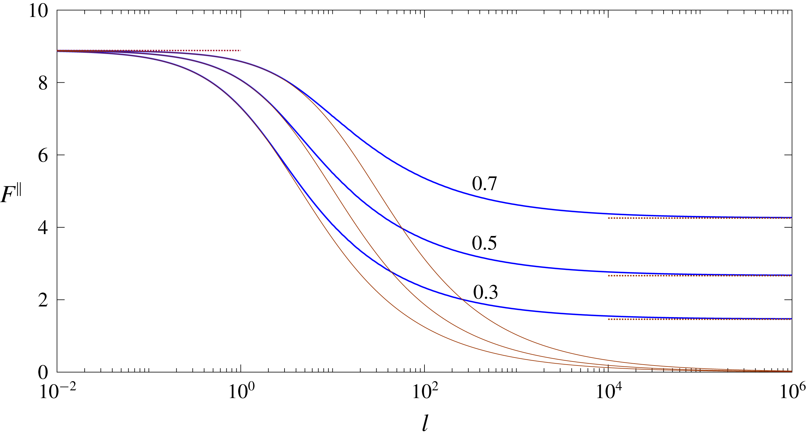
Figure 5. Variation with
 $l$
of the scaled drag
$l$
of the scaled drag
 $F^{\Vert }$
for the indicated values of
$F^{\Vert }$
for the indicated values of
 $\unicode[STIX]{x1D719}$
. The solid curves depict the exact variation, as obtained from (6.12). The dotted lines portray the small- and large-
$\unicode[STIX]{x1D719}$
. The solid curves depict the exact variation, as obtained from (6.12). The dotted lines portray the small- and large-
 $l$
approximations (6.14b
) and (6.16b
). Also shown (thin solid curves) are the Navier-slip approximations, obtained using (B 4) and (B 6).
$l$
approximations (6.14b
) and (6.16b
). Also shown (thin solid curves) are the Navier-slip approximations, obtained using (B 4) and (B 6).
7 Rotation
7.1 Integral mass balance
In the case of rotation about the cylinder axis, it is evident that the
 $z$
-averaged flux through the gap is constant in the
$z$
-averaged flux through the gap is constant in the
 $x,y,z$
reference frame. Denoting this flux by
$x,y,z$
reference frame. Denoting this flux by
 ${\mathcal{F}}$
, integral mass conservation now reads (cf. (6.1))
${\mathcal{F}}$
, integral mass conservation now reads (cf. (6.1))
 $$\begin{eqnarray}l^{-1}\int _{0}^{l}\text{d}Z\int _{0}^{H(X)}\,\text{d}YU(X,Y,Z)={\mathcal{F}}.\end{eqnarray}$$
Substituting (4.3) yields
 $$\begin{eqnarray}\frac{\text{d}P}{\text{d}X}=\frac{{\mathcal{Q}}_{B}(H(X),l,\unicode[STIX]{x1D719})-{\mathcal{F}}}{{\mathcal{Q}}_{P}(H(X),l,\unicode[STIX]{x1D719})},\end{eqnarray}$$
which, as expected, is even in
 $X$
.
$X$
.
As in the case of parallel translation, the flux
 ${\mathcal{F}}$
is determined using (6.3). Changing to the integration variable
${\mathcal{F}}$
is determined using (6.3). Changing to the integration variable
 ${\mathcal{H}}=H(X)$
and making use of the transformations (4.15) and (4.23) gives here (cf. (6.4))
${\mathcal{H}}=H(X)$
and making use of the transformations (4.15) and (4.23) gives here (cf. (6.4))
 $$\begin{eqnarray}{\mathcal{F}}=\left(\int _{1}^{\infty }\frac{\text{d}{\mathcal{H}}}{{\mathcal{H}}^{3}\sqrt{{\mathcal{H}}-1}\,\tilde{{\mathcal{Q}}}_{P}(l/{\mathcal{H}},\unicode[STIX]{x1D719})}\right)^{-1}\int _{1}^{\infty }\frac{\tilde{{\mathcal{Q}}}_{B}(l/{\mathcal{H}},\unicode[STIX]{x1D719})\,\text{d}{\mathcal{H}}}{{\mathcal{H}}^{2}\sqrt{{\mathcal{H}}-1}\,\tilde{{\mathcal{Q}}}_{P}(l/{\mathcal{H}},\unicode[STIX]{x1D719})}.\end{eqnarray}$$
7.2 Resistance
The averaged resistance coefficient
 $T$
(see (2.2b
) and (3.14c
)) is
$T$
(see (2.2b
) and (3.14c
)) is
 $$\begin{eqnarray}T=l^{-1}\int _{0}^{l}\text{d}Z\int _{-\infty }^{\infty }\text{d}X\left.\frac{\unicode[STIX]{x2202}U}{\unicode[STIX]{x2202}Y}\right|_{Y=H(X)}.\end{eqnarray}$$
(This expression is the same as (6.5), but now with the velocity component
 $U$
appropriate to the rotation problem.) Substituting (4.3) and making use of the symmetry of
$U$
appropriate to the rotation problem.) Substituting (4.3) and making use of the symmetry of
 $\text{d}P/\text{d}X$
yields
$\text{d}P/\text{d}X$
yields
 $$\begin{eqnarray}T=-2\int _{0}^{\infty }\text{d}X\,\frac{\text{d}P}{\text{d}X}{\mathcal{S}}_{P}(H(X),l,\unicode[STIX]{x1D719})+2\int _{0}^{\infty }\text{d}X\,{\mathcal{S}}_{B}(H(X),l,\unicode[STIX]{x1D719}),\end{eqnarray}$$
namely the same expression as (6.6), but now with
 $\text{d}P/\text{d}X$
given by (7.2). Substituting (7.2) and changing to the integration variable
$\text{d}P/\text{d}X$
given by (7.2). Substituting (7.2) and changing to the integration variable
 ${\mathcal{H}}=H(X)$
yields, upon making use of transformations (4.15) and (4.23),
${\mathcal{H}}=H(X)$
yields, upon making use of transformations (4.15) and (4.23),
 $$\begin{eqnarray}T=-2^{1/2}\int _{1}^{\infty }\frac{({\mathcal{H}}\tilde{{\mathcal{Q}}}_{B}(l/{\mathcal{H}},\unicode[STIX]{x1D719})-{\mathcal{F}})\tilde{{\mathcal{S}}}_{P}(l/{\mathcal{H}},\unicode[STIX]{x1D719})}{\tilde{{\mathcal{Q}}}_{P}(l/{\mathcal{H}},\unicode[STIX]{x1D719}){\mathcal{H}}^{2}\sqrt{{\mathcal{H}}-1}}\,\text{d}{\mathcal{H}}+2^{1/2}\int _{1}^{\infty }\frac{\tilde{{\mathcal{S}}}_{B}(l/{\mathcal{H}},\unicode[STIX]{x1D719})}{{\mathcal{H}}\sqrt{{\mathcal{H}}-1}}\,\text{d}{\mathcal{H}}.\end{eqnarray}$$
7.3 Limiting values
In the case of rotation about a solid boundary, where
 $\unicode[STIX]{x1D719}=1$
, substitution into (7.3) of (4.25a
) and (4.35a
) gives
$\unicode[STIX]{x1D719}=1$
, substitution into (7.3) of (4.25a
) and (4.35a
) gives
 ${\mathcal{F}}=2/3$
. We then find from (7.6) that
${\mathcal{F}}=2/3$
. We then find from (7.6) that
 $$\begin{eqnarray}\lim _{\unicode[STIX]{x1D719}\rightarrow 1}T=2\sqrt{2}\unicode[STIX]{x03C0},\end{eqnarray}$$
in agreement with the classical results of Jeffrey & Onishi (Reference Jeffrey and Onishi1981). In the case of rotation about a free surface, where
 $\unicode[STIX]{x1D719}=0$
, substitution into (7.3) of (4.27) and (4.37a
) gives
$\unicode[STIX]{x1D719}=0$
, substitution into (7.3) of (4.27) and (4.37a
) gives
 ${\mathcal{F}}=4/3$
. We then find from (7.6) that
${\mathcal{F}}=4/3$
. We then find from (7.6) that
 $$\begin{eqnarray}\lim _{\unicode[STIX]{x1D719}\rightarrow 0}T=\unicode[STIX]{x03C0}\sqrt{2},\end{eqnarray}$$
in agreement with Kaynan & Yariv (Reference Kaynan and Yariv2017).
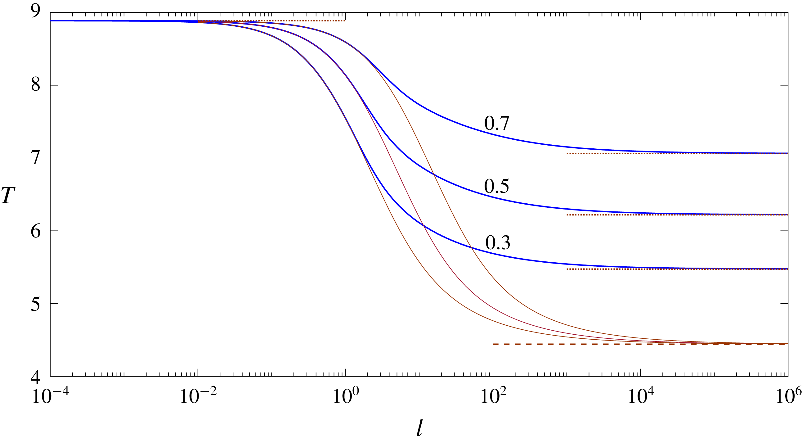
Figure 6. Variation with
 $l$
of the scaled torque
$l$
of the scaled torque
 $T$
for the indicated values of
$T$
for the indicated values of
 $\unicode[STIX]{x1D719}$
. The solid curves depict the exact variation, as obtained from (7.6). The dashed line displays the drag value (7.8) which corresponds to rotation about a free surface, while the dotted lines portray the small- and large-
$\unicode[STIX]{x1D719}$
. The solid curves depict the exact variation, as obtained from (7.6). The dashed line displays the drag value (7.8) which corresponds to rotation about a free surface, while the dotted lines portray the small- and large-
 $l$
approximations (7.9) and (7.10). Also shown (thin solid curves) are the Navier-slip approximations, obtained using (B 4) and (B 8).
$l$
approximations (7.9) and (7.10). Also shown (thin solid curves) are the Navier-slip approximations, obtained using (B 4) and (B 8).
The small-
 $l$
limit coincides with that of a no-slip wall, namely
$l$
limit coincides with that of a no-slip wall, namely
 $$\begin{eqnarray}\lim _{l\rightarrow 0}T=2\sqrt{2}\unicode[STIX]{x03C0}.\end{eqnarray}$$
This limit does not commute with (7.8). For large
 $l$
, substituting into (7.3) of (4.32)–(4.33) and (4.41)–(4.42) yields
$l$
, substituting into (7.3) of (4.32)–(4.33) and (4.41)–(4.42) yields
 $\lim _{l\rightarrow \infty }{\mathcal{F}}=2(2-\unicode[STIX]{x1D719})/3$
. We then find from (7.6) that
$\lim _{l\rightarrow \infty }{\mathcal{F}}=2(2-\unicode[STIX]{x1D719})/3$
. We then find from (7.6) that
 $$\begin{eqnarray}\lim _{l\rightarrow \infty }T=\frac{2\unicode[STIX]{x03C0}\sqrt{2}(2-\unicode[STIX]{x1D719}^{2})}{4-3\unicode[STIX]{x1D719}}.\end{eqnarray}$$
7.4 Arbitrary values of
$l$
and
$\unicode[STIX]{x1D719}$


To evaluate
 $T$
for arbitrary values of
$T$
for arbitrary values of
 $l$
and
$l$
and
 $\unicode[STIX]{x1D719}$
, we plug the entire
$\unicode[STIX]{x1D719}$
, we plug the entire
 $l$
variation of the standard-cell quantities (
$l$
variation of the standard-cell quantities (
 $\tilde{{\mathcal{Q}}}_{P}$
,
$\tilde{{\mathcal{Q}}}_{P}$
,
 $\tilde{{\mathcal{S}}}_{P}$
,
$\tilde{{\mathcal{S}}}_{P}$
,
 $\tilde{{\mathcal{Q}}}_{B}$
and
$\tilde{{\mathcal{Q}}}_{B}$
and
 $\tilde{{\mathcal{S}}}_{B}$
) into (7.3) and (7.6). The results are shown in figure 6.
$\tilde{{\mathcal{S}}}_{B}$
) into (7.3) and (7.6). The results are shown in figure 6.
8 Concluding remarks
We have studied the lubrication interaction between a solid cylinder, moving and rotating arbitrarily in the plane normal to its axis, and a nearby textured (superhydrophobic) surface. Starting from a first-principles microscale formulation, we have systematically developed an asymptotically equivalent macroscale model which, in turn, has allowed us to calculate the hydrodynamic loads exerted on the cylinder. The (slowly varying) lumped parameters appearing in the macroscale description are obtained by solving two auxiliary cell problems, both involving a straight channel where the upper boundary is solid and the lower one is textured. In the first cell problem, the flow is driven by a unit pressure gradient, with the boundaries of the channel fixed. In the second cell problem, there is no pressure gradient; rather, the flow is generated by parallel motion of the upper boundary with unit speed.
It turns out that the case of squeeze flow due to perpendicular particle motion is special in that it is affected only by the first, pressure-driven, cell problem. In particular, the drag on the cylinder in that case is given by a quadrature of a nonlinear function of a single lumped parameter: the averaged cross-sectional volumetric flux in the pressure-driven cell problem. We note that it is possible to mathematically recast the latter flux as the effective slip length used in the lubrication models discussed in the introduction. In contrast, the case of general rigid-body motion is affected by both the pressure-driven and boundary-driven cell problems. In fact, we have seen that calculating the hydrodynamic loads in the cases of parallel translation and rotation requires knowledge of two lumped parameters for each of the cell problems: in addition to the averaged flux, one requires an averaged shear stress. Thus, the heuristic effective-slip models used to study squeeze-flow interactions cannot be applied to lubrication interactions involving parallel motion.
It is useful to recapitulate the different approaches used to model lubrication interactions between solid bodies moving relative to nearby textured surfaces. The Navier-slip models, where the slip length is an intrinsic surface property, apply for all modes of relative motions, but are restricted to gaps that are large compared to the texture period. The effective-slip model, where the slip length is related to the mean flux in a pressure-driven cell problem, applies in principle to both large and small gaps, but is limited to perpendicular motion between the two surfaces. The present approach has none of the above limitations and demonstrates a systematic framework where the appropriate macroscale model is developed from first principles using asymptotic tools.
Our analysis shows that, when the clearance between the cylinder and the textured surface is comparable to the period of the textured surface, the dependences of the hydrodynamic loads on the clearance exhibit none of the classical power laws familiar from classical lubrication theory. We illustrate this feature in appendix D by considering the unsteady mobility problem of a cylinder sedimenting towards a textured surface under the action of a uniform force field. In light of the above, we find a non-power-law dependence of the clearance on time, qualitatively similar to the observations of Chastel & Mongruel (Reference Chastel and Mongruel2016) in the case of a solid sphere sedimenting towards a wetted textured substrate.
In the configuration studied in this part, where the cylinder axis is perpendicular to the grooves, the geometry is periodic along the direction of that axis, on which the microstructure varies rapidly. The three modes of rigid-body motion considered herein are consistent with that orthogonality. The inherent periodicity has allowed for a natural separation of the fast variation associated with the patterned surface from the slow variation of the lubricating flow field associated with the cylinder curvature. In the complementary configuration, where the cylinder axis is parallel to the grooves, the geometry is no longer periodic. As a consequence, the fast and slow variations take place along the same direction, hence the above-mentioned separation no longer applies. Nonetheless, it is evident that an analogous separation can be achieved using a systematic combination of multiple-scale theory with a lubrication approximation. This will be the subject of the second part in this sequence.
Acknowledgements
E.Y. was supported by the Israel Science Foundation (grant no. 1081/16).
Appendix A. Stokes-flow reciprocity
Consider a rigid particle of arbitrary shape that undergoes a rigid-body motion within a viscous liquid (viscosity
 $\unicode[STIX]{x1D707}$
). The particle motion is completely described by the rectilinear velocity
$\unicode[STIX]{x1D707}$
). The particle motion is completely described by the rectilinear velocity
 $\boldsymbol{s}$
of an arbitrary material point
$\boldsymbol{s}$
of an arbitrary material point
 $O$
, fixed in the body, and the angular velocity
$O$
, fixed in the body, and the angular velocity
 $\unicode[STIX]{x1D74E}$
. The linearity of the Stokes equations implies that the hydrodynamic force and torque (about
$\unicode[STIX]{x1D74E}$
. The linearity of the Stokes equations implies that the hydrodynamic force and torque (about
 $O$
) are of the respective forms
$O$
) are of the respective forms
 $$\begin{eqnarray}-\unicode[STIX]{x1D707}(\unicode[STIX]{x1D641}\boldsymbol{\cdot }\boldsymbol{s}+\unicode[STIX]{x1D63F}\boldsymbol{\cdot }\unicode[STIX]{x1D74E}),\quad -\unicode[STIX]{x1D707}(\unicode[STIX]{x1D63E}\boldsymbol{\cdot }\boldsymbol{s}+\unicode[STIX]{x1D64F}\boldsymbol{\cdot }\unicode[STIX]{x1D74E}),\end{eqnarray}$$
where the resistance dyadics appearing therein are intrinsic geometric properties of the particle, dependent only on its size and shape. Happel & Brenner (Reference Happel and Brenner1965) proved that the coupling tensors
 $\unicode[STIX]{x1D63E}$
and
$\unicode[STIX]{x1D63E}$
and
 $\unicode[STIX]{x1D63F}$
are related as
$\unicode[STIX]{x1D63F}$
are related as
 $$\begin{eqnarray}\unicode[STIX]{x1D63F}=\unicode[STIX]{x1D63E}^{\dagger }.\end{eqnarray}$$
The proof given by Happel & Brenner (Reference Happel and Brenner1965) makes use of the assumption that the particle moves in an unbounded fluid domain. We here extend their proof to the case where the particle moves in the vicinity of a compound planar surface consisting of both no-slip and shear-free patches.
The velocity field
 $\boldsymbol{v}$
is governed by the continuity and Stokes equations, the no-slip condition on the particle,
$\boldsymbol{v}$
is governed by the continuity and Stokes equations, the no-slip condition on the particle,
 $$\begin{eqnarray}\boldsymbol{v}=\boldsymbol{s}+\unicode[STIX]{x1D74E}\times \boldsymbol{x},\end{eqnarray}$$
and the condition of far-field decay. In addition,
 $\boldsymbol{v}$
satisfies homogeneous conditions on the adjacent surface, which take the form of either the no-slip condition,
$\boldsymbol{v}$
satisfies homogeneous conditions on the adjacent surface, which take the form of either the no-slip condition,
 $$\begin{eqnarray}\boldsymbol{v}=\mathbf{0},\end{eqnarray}$$
or the impermeability and shear-free conditions,
 $$\begin{eqnarray}\hat{\boldsymbol{n}}\boldsymbol{\cdot }\boldsymbol{v}=\mathbf{0},\quad \hat{\boldsymbol{n}}\boldsymbol{\cdot }\unicode[STIX]{x1D748}\boldsymbol{\cdot }\hat{\boldsymbol{t}}=0.\end{eqnarray}$$
Here
 $\hat{\boldsymbol{n}}$
is a unit vector normal to the surface (say, pointing into the liquid),
$\hat{\boldsymbol{n}}$
is a unit vector normal to the surface (say, pointing into the liquid),
 $\hat{\boldsymbol{t}}$
may be any unit vector that is parallel to the surface at the point considered, and
$\hat{\boldsymbol{t}}$
may be any unit vector that is parallel to the surface at the point considered, and
 $\unicode[STIX]{x1D748}$
is the stress field.
$\unicode[STIX]{x1D748}$
is the stress field.
In what follows we exploit linearity and decompose
 $\boldsymbol{v}$
as
$\boldsymbol{v}$
as
 $\boldsymbol{v}^{\prime }+\boldsymbol{v}^{\prime \prime }$
, with the stress field respectively decomposed as
$\boldsymbol{v}^{\prime }+\boldsymbol{v}^{\prime \prime }$
, with the stress field respectively decomposed as
 $\unicode[STIX]{x1D748}=\unicode[STIX]{x1D748}^{\prime }+\unicode[STIX]{x1D748}^{\prime \prime }$
. Both
$\unicode[STIX]{x1D748}=\unicode[STIX]{x1D748}^{\prime }+\unicode[STIX]{x1D748}^{\prime \prime }$
. Both
 $(\boldsymbol{v}^{\prime },\unicode[STIX]{x1D748}^{\prime })$
and
$(\boldsymbol{v}^{\prime },\unicode[STIX]{x1D748}^{\prime })$
and
 $(\boldsymbol{v}^{\prime \prime },\unicode[STIX]{x1D748}^{\prime \prime })$
satisfy the homogeneous conditions and differential equations that govern the original flow
$(\boldsymbol{v}^{\prime \prime },\unicode[STIX]{x1D748}^{\prime \prime })$
satisfy the homogeneous conditions and differential equations that govern the original flow
 $(\boldsymbol{v},\unicode[STIX]{x1D748})$
. They differ in the conditions satisfied at the particle surface, where (A 3) is decomposed as
$(\boldsymbol{v},\unicode[STIX]{x1D748})$
. They differ in the conditions satisfied at the particle surface, where (A 3) is decomposed as
 $$\begin{eqnarray}\boldsymbol{v}^{\prime }=\boldsymbol{s},\quad \boldsymbol{v}^{\prime \prime }=\unicode[STIX]{x1D74E}\times \boldsymbol{x}.\end{eqnarray}$$
The starting point is Lorentz’s reciprocal theorem (Happel & Brenner Reference Happel and Brenner1965), applied to the subfields
 $(\boldsymbol{v}^{\prime },\unicode[STIX]{x1D748}^{\prime })$
and
$(\boldsymbol{v}^{\prime },\unicode[STIX]{x1D748}^{\prime })$
and
 $(\boldsymbol{v}^{\prime \prime },\unicode[STIX]{x1D748}^{\prime \prime })$
,
$(\boldsymbol{v}^{\prime \prime },\unicode[STIX]{x1D748}^{\prime \prime })$
,
 $$\begin{eqnarray}\int \text{d}A\;\hat{\boldsymbol{n}}\boldsymbol{\cdot }\unicode[STIX]{x1D748}^{\prime \prime }\boldsymbol{\cdot }\boldsymbol{v}^{\prime }=\int \text{d}A\;\hat{\boldsymbol{n}}\boldsymbol{\cdot }\unicode[STIX]{x1D748}^{\prime }\boldsymbol{\cdot }\boldsymbol{v}^{\prime \prime }.\end{eqnarray}$$
Here, the integration domain consists of both the particle boundary and the compound surface, on which the unit normal
 $\hat{\boldsymbol{n}}$
is also pointing into the liquid. (Assuming sufficient decay rate, the contribution from the fluid boundary at ‘infinity’ trivially vanishes.)
$\hat{\boldsymbol{n}}$
is also pointing into the liquid. (Assuming sufficient decay rate, the contribution from the fluid boundary at ‘infinity’ trivially vanishes.)
Since both
 $\boldsymbol{v}^{\prime }$
and
$\boldsymbol{v}^{\prime }$
and
 $\boldsymbol{v}^{\prime \prime }$
vanish at the no-slip patches, these regions do not contribute to the integrals appearing in (A 7). Consider now the shear-free patches. Since
$\boldsymbol{v}^{\prime \prime }$
vanish at the no-slip patches, these regions do not contribute to the integrals appearing in (A 7). Consider now the shear-free patches. Since
 $\boldsymbol{v}^{\prime }$
satisfies there the impermeability condition (A 5a
), it may be written as
$\boldsymbol{v}^{\prime }$
satisfies there the impermeability condition (A 5a
), it may be written as
 $\hat{\boldsymbol{t}}\,|\boldsymbol{v}^{\prime }|$
. Making use of the shear-free condition (A 5b
), we then find that these patches do not contribute to the integral appearing on the left-hand side of (A 7). Similar arguments apply to the integral appearing on the right-hand side of (A 7). We conclude that (A 7) applies with the integration domain being the particle boundary. At this stage we can simply follow the proof as outlined by Happel & Brenner (Reference Happel and Brenner1965).
$\hat{\boldsymbol{t}}\,|\boldsymbol{v}^{\prime }|$
. Making use of the shear-free condition (A 5b
), we then find that these patches do not contribute to the integral appearing on the left-hand side of (A 7). Similar arguments apply to the integral appearing on the right-hand side of (A 7). We conclude that (A 7) applies with the integration domain being the particle boundary. At this stage we can simply follow the proof as outlined by Happel & Brenner (Reference Happel and Brenner1965).
Consider now the problem formulated in § 2, involving an infinite circular cylinder of radius
 $a$
near a periodic array of alternating no-slip and shear-free strips. When the cylinder axis is perpendicular to these stripes, the geometry is periodic, and this periodicity is consistent with the rigid-body motion
$a$
near a periodic array of alternating no-slip and shear-free strips. When the cylinder axis is perpendicular to these stripes, the geometry is periodic, and this periodicity is consistent with the rigid-body motion
 $$\begin{eqnarray}\boldsymbol{s}=\hat{\boldsymbol{e}}_{x}s^{\Vert }+\hat{\boldsymbol{e}}_{y}s^{\bot },\quad \unicode[STIX]{x1D74E}=\hat{\boldsymbol{e}}_{z}\unicode[STIX]{x1D714},\end{eqnarray}$$
considered in § 2. The linearity of the Stokes equations implies that expressions (A 1) still hold, provided they are now understood to represent respectively the force and torque (about the cylinder axis) per unit length of the cylinder axis, averaged over a single period of the superhydrophobic surface. The extension of the preceding proof to this geometry is straightforward and need not be repeated; we therefore conclude that (A 2) applies here as well.
Making use of the Cartesian coordinates of § 2, the only fixed vectors provided by the geometry considered in that section are
 $\hat{\boldsymbol{e}}_{y}$
, the unit vector perpendicular to the superhydrophobic surface, and
$\hat{\boldsymbol{e}}_{y}$
, the unit vector perpendicular to the superhydrophobic surface, and
 $\hat{\boldsymbol{e}}_{z}$
, the unit vector in the periodicity direction. Since the averaged force and torque are necessarily independent of the latter, the true tensors
$\hat{\boldsymbol{e}}_{z}$
, the unit vector in the periodicity direction. Since the averaged force and torque are necessarily independent of the latter, the true tensors
 $\unicode[STIX]{x1D641}$
and
$\unicode[STIX]{x1D641}$
and
 $\unicode[STIX]{x1D64F}$
must therefore adopt the respective forms
$\unicode[STIX]{x1D64F}$
must therefore adopt the respective forms
 $$\begin{eqnarray}\unicode[STIX]{x1D641}=\hat{\boldsymbol{e}}_{y}\hat{\boldsymbol{e}}_{y}\,f^{\bot }+(\unicode[STIX]{x1D644}-\hat{\boldsymbol{e}}_{y}\hat{\boldsymbol{e}}_{y})\,f^{\Vert },\quad \unicode[STIX]{x1D64F}=a^{2}[\hat{\boldsymbol{e}}_{y}\hat{\boldsymbol{e}}_{y}t^{\bot }+(\unicode[STIX]{x1D644}-\hat{\boldsymbol{e}}_{y}\hat{\boldsymbol{e}}_{y})t^{\Vert }],\end{eqnarray}$$
while the pseudo-tensor
 $\unicode[STIX]{x1D63E}$
is of the form
$\unicode[STIX]{x1D63E}$
is of the form
 $$\begin{eqnarray}\unicode[STIX]{x1D63E}=\unicode[STIX]{x1D750}\boldsymbol{\cdot }\hat{\boldsymbol{e}}_{y}\,ac,\end{eqnarray}$$
in which
 $\unicode[STIX]{x1D750}$
is the isotropic triadic. (The introduction of
$\unicode[STIX]{x1D750}$
is the isotropic triadic. (The introduction of
 $a$
into expressions (A 9) and (A 10) renders the pertinent resistance coefficients dimensionless.) Substitution of (A 8), (A 9) and (A 10) into (A 1) and making use of (A 2) readily yields (2.1) and (2.2), where we simply write
$a$
into expressions (A 9) and (A 10) renders the pertinent resistance coefficients dimensionless.) Substitution of (A 8), (A 9) and (A 10) into (A 1) and making use of (A 2) readily yields (2.1) and (2.2), where we simply write
 $t$
instead of
$t$
instead of
 $t^{\Vert }$
.
$t^{\Vert }$
.
Appendix B. Navier-slip approach
A common methodology for handling microstructured surfaces involves replacing the exact dynamic conditions (2.7) and (2.8) at
 $y=0$
by the coarse-grained Navier conditions,
$y=0$
by the coarse-grained Navier conditions,
 $$\begin{eqnarray}u=b^{\Vert }\frac{\unicode[STIX]{x2202}u}{\unicode[STIX]{x2202}z},\quad w=b^{\bot }\frac{\unicode[STIX]{x2202}w}{\unicode[STIX]{x2202}z},\end{eqnarray}$$
wherein
 $b^{\Vert }$
and
$b^{\Vert }$
and
 $b^{\bot }$
are the respective slip lengths (normalised by
$b^{\bot }$
are the respective slip lengths (normalised by
 $a$
) appropriate for an imposed shear flow parallel and perpendicular to the grooves. In the present configuration of flat menisci, the parallel and perpendicular slip coefficients have been respectively obtained by Philip (Reference Philip1972a
) as
$a$
) appropriate for an imposed shear flow parallel and perpendicular to the grooves. In the present configuration of flat menisci, the parallel and perpendicular slip coefficients have been respectively obtained by Philip (Reference Philip1972a
) as
 $b$
and
$b$
and
 $b/2$
, wherein
$b/2$
, wherein
 $$\begin{eqnarray}b=\frac{2lh}{\unicode[STIX]{x03C0}}\ln \sec \frac{\unicode[STIX]{x03C0}(1-\unicode[STIX]{x1D719})}{2}.\end{eqnarray}$$
Since
 $w$
trivially vanishes here, conditions (B 1) are equivalent to those pertinent for an isotropic surface of slip length
$w$
trivially vanishes here, conditions (B 1) are equivalent to those pertinent for an isotropic surface of slip length
 $b$
.
$b$
.
In the inner region, where the
 $z$
-coordinate is rescaled by
$z$
-coordinate is rescaled by
 $h$
(see (3.1c
)), the exact conditions (3.8) and (3.9) are accordingly replaced by the Robin condition
$h$
(see (3.1c
)), the exact conditions (3.8) and (3.9) are accordingly replaced by the Robin condition
 $$\begin{eqnarray}U=B\frac{\unicode[STIX]{x2202}U}{\unicode[STIX]{x2202}Z}\quad \text{at }Z=0,\end{eqnarray}$$
where
 $$\begin{eqnarray}B=\frac{2l}{\unicode[STIX]{x03C0}}\ln \sec \frac{\unicode[STIX]{x03C0}(1-\unicode[STIX]{x1D719})}{2}.\end{eqnarray}$$
The resulting near-contact problem of a cylinder that moves in the vicinity of an isotropic slippery surface, described by conditions (3.7) and (B 3), has been solved by Kaynan & Yariv (Reference Kaynan and Yariv2017), who provide the following expressions for the leading-order drag coefficients (defined in (3.13) and (3.14)):
 $$\begin{eqnarray}\displaystyle & \displaystyle F^{\bot }=\frac{3\unicode[STIX]{x03C0}}{4\sqrt{2}B^{2}}(3+6B+2B^{2}-3\sqrt{1+4B}), & \displaystyle\end{eqnarray}$$
 $$\begin{eqnarray}\displaystyle & \displaystyle F^{\Vert }=4\sqrt{2}\unicode[STIX]{x03C0}\frac{(1+2B+2B^{2})\sqrt{1+4B}-1-4B}{\sqrt{1+4B}-1-2B+10B^{2}+8B^{3}}, & \displaystyle\end{eqnarray}$$
 $$\begin{eqnarray}\displaystyle & \displaystyle C=-2\sqrt{2}\unicode[STIX]{x03C0}\frac{1+6B+8B^{2}-(1+4B+2B^{2})\sqrt{1+4B}}{1+2B-10B^{2}-8B^{3}-\sqrt{1+4B}}, & \displaystyle\end{eqnarray}$$
 $$\begin{eqnarray}\displaystyle & \displaystyle T=2\sqrt{2}\unicode[STIX]{x03C0}(2+B)\frac{4B^{2}-3B-1+(B+1)\sqrt{1+4B}}{8B^{3}+10B^{2}-2B-1+\sqrt{1+4B}}. & \displaystyle\end{eqnarray}$$
With
 $B$
being proportional to
$B$
being proportional to
 $l$
, formulae (B 5)–(B 8) represent, upon an appropriate contraction, the variation of the drag coefficients with
$l$
, formulae (B 5)–(B 8) represent, upon an appropriate contraction, the variation of the drag coefficients with
 $l$
for any value of
$l$
for any value of
 $\unicode[STIX]{x1D719}$
. Now, according to the Navier model (B 3), the large-
$\unicode[STIX]{x1D719}$
. Now, according to the Navier model (B 3), the large-
 $B$
limit represents an approach to a free surface. It is clear, however, that the very concept of a slip length breaks down in the large-
$B$
limit represents an approach to a free surface. It is clear, however, that the very concept of a slip length breaks down in the large-
 $l$
limit. It follows that the above heuristic approach fails to predict the correct hydrodynamic resistance in that limit. On the other hand, that approach appears plausible in the small-
$l$
limit. It follows that the above heuristic approach fails to predict the correct hydrodynamic resistance in that limit. On the other hand, that approach appears plausible in the small-
 $l$
limit, where the flow in the vicinity of the compound surface
$l$
limit, where the flow in the vicinity of the compound surface
 $Y=0$
corresponds to that of a semi-bounded homogeneous shear about that surface (Kirk, Hodes & Papageorgiou Reference Kirk, Hodes and Papageorgiou2017) – the very situation for which an intrinsic Navier condition is approximately applicable.
$Y=0$
corresponds to that of a semi-bounded homogeneous shear about that surface (Kirk, Hodes & Papageorgiou Reference Kirk, Hodes and Papageorgiou2017) – the very situation for which an intrinsic Navier condition is approximately applicable.
Appendix C. Semi-analytic solution of the standard-cell problems
C.1 Pressure-driven cell problem
The standard-cell flow
 $\tilde{{\mathcal{U}}}_{P}(Y,Z)$
is governed by (4.4)–(4.7), with
$\tilde{{\mathcal{U}}}_{P}(Y,Z)$
is governed by (4.4)–(4.7), with
 ${\mathcal{H}}$
set to unity. The quantities of interest are the corresponding average flux
${\mathcal{H}}$
set to unity. The quantities of interest are the corresponding average flux
 $\tilde{{\mathcal{Q}}}_{P}$
(see (4.8)) and shear
$\tilde{{\mathcal{Q}}}_{P}$
(see (4.8)) and shear
 $\tilde{{\mathcal{S}}}_{P}$
(see (4.9)). It is convenient to solve the ‘flipped’ problem, where the no-slip boundary is at
$\tilde{{\mathcal{S}}}_{P}$
(see (4.9)). It is convenient to solve the ‘flipped’ problem, where the no-slip boundary is at
 $Y^{\prime }=0$
and the compound boundary is at
$Y^{\prime }=0$
and the compound boundary is at
 $Y^{\prime }=1$
, in which
$Y^{\prime }=1$
, in which
 $Y^{\prime }=1-Y$
.
$Y^{\prime }=1-Y$
.
Defining
 $$\begin{eqnarray}\tilde{{\mathcal{U}}}_{P}=-\frac{{Y^{\prime }}^{2}}{2}+\unicode[STIX]{x1D6EC},\end{eqnarray}$$
we find that
 $\unicode[STIX]{x1D6EC}$
is governed by the following:
$\unicode[STIX]{x1D6EC}$
is governed by the following:
(i) Laplace’s equation,
(C 2)$$\begin{eqnarray}\frac{\unicode[STIX]{x2202}^{2}\unicode[STIX]{x1D6EC}}{\unicode[STIX]{x2202}{Y^{\prime }}^{2}}+\frac{\unicode[STIX]{x2202}^{2}\unicode[STIX]{x1D6EC}}{\unicode[STIX]{x2202}Z^{2}}=0\quad \text{for }0<Z<l,~0<Y^{\prime }<1;\end{eqnarray}$$
(ii) the Dirichlet condition,
(C 3)$$\begin{eqnarray}\unicode[STIX]{x1D6EC}=0\quad \text{at }Y^{\prime }=0;\end{eqnarray}$$
(iii) the mixed conditions at
$Y^{\prime }=1$
, (C 4a,b )$$\begin{eqnarray}\unicode[STIX]{x1D6EC}=\frac{1}{2}\quad \text{for }0<Z<\unicode[STIX]{x1D719}l,\quad \frac{\unicode[STIX]{x2202}\unicode[STIX]{x1D6EC}}{\unicode[STIX]{x2202}Y^{\prime }}=1\quad \text{for }\unicode[STIX]{x1D719}l<Z<l;\end{eqnarray}$$


and (iv) the symmetry conditions,
 $$\begin{eqnarray}\frac{\unicode[STIX]{x2202}\unicode[STIX]{x1D6EC}}{\unicode[STIX]{x2202}Z}=0\quad \text{at }Z=0,l.\end{eqnarray}$$
Once
 $\unicode[STIX]{x1D6EC}$
is determined, the flux and mean shear are given by (cf. (4.14))
$\unicode[STIX]{x1D6EC}$
is determined, the flux and mean shear are given by (cf. (4.14))
 $$\begin{eqnarray}\tilde{{\mathcal{Q}}}_{P}=l^{-1}\int _{0}^{l}\text{d}Z\int _{0}^{1}\text{d}Y^{\prime }\,\unicode[STIX]{x1D6EC}(Y^{\prime },Z)-\frac{1}{6},\quad \tilde{{\mathcal{S}}}_{P}=-l^{-1}\int _{0}^{l}\text{d}Z\left.\frac{\unicode[STIX]{x2202}\unicode[STIX]{x1D6EC}}{\unicode[STIX]{x2202}Y^{\prime }}\right|_{Y^{\prime }=0}.\end{eqnarray}$$
The most general solution of (C 2) which satisfies the homogeneous conditions (C 3) and (C 5) is given by the Fourier series
 $$\begin{eqnarray}\unicode[STIX]{x1D6EC}=A_{0}Y^{\prime }+\mathop{\sum }_{n=1}^{\infty }A_{n}\sinh k_{n}Y^{\prime }\cos k_{n}Z,\end{eqnarray}$$
wherein
 $k_{n}=n\unicode[STIX]{x03C0}/l$
. Substitution into (C 6) gives
$k_{n}=n\unicode[STIX]{x03C0}/l$
. Substitution into (C 6) gives
 $\tilde{{\mathcal{Q}}}_{P}=A_{0}/2-1/6$
and
$\tilde{{\mathcal{Q}}}_{P}=A_{0}/2-1/6$
and
 $\tilde{{\mathcal{S}}}_{P}=-A_{0}$
, respectively. To determine
$\tilde{{\mathcal{S}}}_{P}=-A_{0}$
, respectively. To determine
 $\tilde{{\mathcal{Q}}}_{P}$
and
$\tilde{{\mathcal{Q}}}_{P}$
and
 $\tilde{{\mathcal{S}}}_{P}$
we need to calculate the Fourier coefficients
$\tilde{{\mathcal{S}}}_{P}$
we need to calculate the Fourier coefficients
 $\{A_{n}\}_{n=0}^{\infty }$
using the inhomogeneous conditions (C 4). Substitution of (C 7) yields, upon affecting the change of variables
$\{A_{n}\}_{n=0}^{\infty }$
using the inhomogeneous conditions (C 4). Substitution of (C 7) yields, upon affecting the change of variables
 $Z=l\unicode[STIX]{x1D701}$
, the dual series equations
$Z=l\unicode[STIX]{x1D701}$
, the dual series equations
 $$\begin{eqnarray}\displaystyle & \displaystyle A_{0}+\mathop{\sum }_{n=1}^{\infty }A_{n}\sinh k_{n}\cos n\unicode[STIX]{x03C0}\unicode[STIX]{x1D701}=\frac{1}{2}\quad \text{for }0<\unicode[STIX]{x1D701}<\unicode[STIX]{x1D719}, & \displaystyle\end{eqnarray}$$
 $$\begin{eqnarray}\displaystyle & \displaystyle A_{0}+\mathop{\sum }_{n=1}^{\infty }k_{n}A_{n}\cosh k_{n}\cos n\unicode[STIX]{x03C0}\unicode[STIX]{x1D701}=1\quad \text{for }\unicode[STIX]{x1D719}<\unicode[STIX]{x1D701}<1. & \displaystyle\end{eqnarray}$$
By forming the inner product of these equations with
 $\cos m\unicode[STIX]{x03C0}\unicode[STIX]{x1D701}$
(
$\cos m\unicode[STIX]{x03C0}\unicode[STIX]{x1D701}$
(
 $m=0,1,2,\ldots$
) on the interval
$m=0,1,2,\ldots$
) on the interval
 $\unicode[STIX]{x1D701}\in [0,1]$
, we obtain an infinite linear system of equations governing the unknowns
$\unicode[STIX]{x1D701}\in [0,1]$
, we obtain an infinite linear system of equations governing the unknowns
 $\{A_{m}\}_{m=0}^{\infty }$
. Owing to the presence of the hyperbolic functions, the coefficients multiplying these unknowns diverge exponentially fast as
$\{A_{m}\}_{m=0}^{\infty }$
. Owing to the presence of the hyperbolic functions, the coefficients multiplying these unknowns diverge exponentially fast as
 $m$
increases. It is therefore convenient to employ the scaled coefficients
$m$
increases. It is therefore convenient to employ the scaled coefficients
 $\tilde{A}_{n}=A_{n}\cosh k_{n}$
(see Lauga & Stone Reference Lauga and Stone2003). These are readily obtained using controlled truncation.
$\tilde{A}_{n}=A_{n}\cosh k_{n}$
(see Lauga & Stone Reference Lauga and Stone2003). These are readily obtained using controlled truncation.
C.2 Boundary-driven cell problem
Consider next the boundary-driven standard-cell flow
 $\tilde{{\mathcal{U}}}_{B}(Y,Z)$
, with the goal of calculating the average properties
$\tilde{{\mathcal{U}}}_{B}(Y,Z)$
, with the goal of calculating the average properties
 $\tilde{Q}_{B}$
and
$\tilde{Q}_{B}$
and
 $\tilde{S}_{B}$
. Defining
$\tilde{S}_{B}$
. Defining
 $$\begin{eqnarray}\tilde{{\mathcal{U}}}_{B}(Y,Z)=1-Y^{\prime }+\unicode[STIX]{x1D6EC}(Y^{\prime },Z),\end{eqnarray}$$
where
 $Y^{\prime }=1-Y$
, we find that
$Y^{\prime }=1-Y$
, we find that
 $\unicode[STIX]{x1D6EC}$
is governed by the following:
$\unicode[STIX]{x1D6EC}$
is governed by the following:
(i) Laplace’s equation,
(C 10)$$\begin{eqnarray}\frac{\unicode[STIX]{x2202}^{2}\unicode[STIX]{x1D6EC}}{\unicode[STIX]{x2202}{Y^{\prime }}^{2}}+\frac{\unicode[STIX]{x2202}^{2}\unicode[STIX]{x1D6EC}}{\unicode[STIX]{x2202}Z^{2}}=0\quad \text{for }0<Z<l,~0<Y^{\prime }<1;\end{eqnarray}$$
(ii) the Dirichlet condition,
(C 11)$$\begin{eqnarray}\unicode[STIX]{x1D6EC}=0\quad \text{at }Y^{\prime }=0;\end{eqnarray}$$
(iii) the mixed conditions at
$Y^{\prime }=1$
, (C 12a,b )$$\begin{eqnarray}\unicode[STIX]{x1D6EC}=0\quad \text{for }0<Z<\unicode[STIX]{x1D719}l,\quad \frac{\unicode[STIX]{x2202}\unicode[STIX]{x1D6EC}}{\unicode[STIX]{x2202}Y^{\prime }}=1\quad \text{for }\unicode[STIX]{x1D719}l<Z<l;\end{eqnarray}$$


and (iv) the symmetry conditions,
 $$\begin{eqnarray}\frac{\unicode[STIX]{x2202}\unicode[STIX]{x1D6EC}}{\unicode[STIX]{x2202}Z}=0\quad \text{at }Z=0,l.\end{eqnarray}$$
Once
 $\unicode[STIX]{x1D6EC}$
is determined, the flux and mean shear are given by
$\unicode[STIX]{x1D6EC}$
is determined, the flux and mean shear are given by
 $$\begin{eqnarray}\tilde{{\mathcal{Q}}}_{B}=l^{-1}\int _{0}^{l}\text{d}Z\int _{0}^{1}\text{d}Y^{\prime }\,\unicode[STIX]{x1D6EC}(Y^{\prime },Z)+\frac{1}{2},\quad \tilde{{\mathcal{S}}}_{B}=1-l^{-1}\int _{0}^{l}\text{d}Z\left.\frac{\unicode[STIX]{x2202}\unicode[STIX]{x1D6EC}}{\unicode[STIX]{x2202}Y^{\prime }}\right|_{Y^{\prime }=0}.\end{eqnarray}$$
The solution for
 $\unicode[STIX]{x1D6EC}$
is again of the form (C 7), where now the Fourier coefficients satisfy the dual series equations
$\unicode[STIX]{x1D6EC}$
is again of the form (C 7), where now the Fourier coefficients satisfy the dual series equations
 $$\begin{eqnarray}\displaystyle & \displaystyle A_{0}+\mathop{\sum }_{n=1}^{\infty }A_{n}\sinh k_{n}\cos n\unicode[STIX]{x03C0}\unicode[STIX]{x1D701}=0\quad \text{for }0<\unicode[STIX]{x1D701}<\unicode[STIX]{x1D719}, & \displaystyle\end{eqnarray}$$
 $$\begin{eqnarray}\displaystyle & \displaystyle A_{0}+\mathop{\sum }_{n=1}^{\infty }k_{n}A_{n}\cosh k_{n}\cos n\unicode[STIX]{x03C0}\unicode[STIX]{x1D701}=1\quad \text{for }\unicode[STIX]{x1D719}<\unicode[STIX]{x1D701}<1. & \displaystyle\end{eqnarray}$$
Once solved, following the method described for the pressure-driven cell problem, the average flux and shear are obtained as
 $\tilde{{\mathcal{Q}}}_{B}=A_{0}/2+1/2$
and
$\tilde{{\mathcal{Q}}}_{B}=A_{0}/2+1/2$
and
 $\tilde{{\mathcal{S}}}_{B}=1-A_{0}$
.
$\tilde{{\mathcal{S}}}_{B}=1-A_{0}$
.
Appendix D. Sedimentation: breakdown of
$h^{-3/2}$
drag scaling

In our dimensionless notation, where length variables are normalised by
 $a$
, the period of the microstructure has been denoted
$a$
, the period of the microstructure has been denoted
 $2lh$
, where
$2lh$
, where
 $h$
is the instantaneous clearance. Since the period is a fixed quantity, this notation necessitates that
$h$
is the instantaneous clearance. Since the period is a fixed quantity, this notation necessitates that
 $l$
varies with time when considering an unsteady process for which
$l$
varies with time when considering an unsteady process for which
 $h$
diminishes with time. In that case it is convenient to define the period as
$h$
diminishes with time. In that case it is convenient to define the period as
 $2\unicode[STIX]{x1D706}h_{0}$
, where
$2\unicode[STIX]{x1D706}h_{0}$
, where
 $h_{0}$
is the value of
$h_{0}$
is the value of
 $h$
at zero time. The scaled period
$h$
at zero time. The scaled period
 $\unicode[STIX]{x1D706}$
is independent of time, while the instantaneous value of
$\unicode[STIX]{x1D706}$
is independent of time, while the instantaneous value of
 $l$
is given by
$l$
is given by
 $$\begin{eqnarray}l=\unicode[STIX]{x1D706}h_{0}/h.\end{eqnarray}$$
Recall also that, in our dimensionless notation, where forces per unit length are normalised by
 $\unicode[STIX]{x1D707}s^{\bot }h^{-1/2}$
, the hydrodynamic drag on the cylinder (per unit length in the
$\unicode[STIX]{x1D707}s^{\bot }h^{-1/2}$
, the hydrodynamic drag on the cylinder (per unit length in the
 $z$
-direction) is, at leading order,
$z$
-direction) is, at leading order,
 $h^{-1}F^{\bot }(l,\unicode[STIX]{x1D719})$
. Making use of (D 1), we find that the dimensional drag (per unit length) is
$h^{-1}F^{\bot }(l,\unicode[STIX]{x1D719})$
. Making use of (D 1), we find that the dimensional drag (per unit length) is
 $$\begin{eqnarray}\unicode[STIX]{x1D707}s^{\bot }\frac{F^{\bot }(\unicode[STIX]{x1D706}h_{0}/h,\unicode[STIX]{x1D719})}{h^{3/2}}.\end{eqnarray}$$
Owing to the dependence of
 $F^{\bot }$
upon
$F^{\bot }$
upon
 $h$
, the drag no longer possesses the classical
$h$
, the drag no longer possesses the classical
 $h^{-3/2}$
power law.
$h^{-3/2}$
power law.
We illustrate the ramifications of this unconventional feature by considering a sedimentation process, assuming a constant (e.g. gravity) external force that pushes the cylinder towards the surface. The dimensional magnitude of the external force (per unit length) is denoted by
 $\unicode[STIX]{x1D707}s_{0}h_{0}^{-3/2}$
. Comparing to (D 2) we note that
$\unicode[STIX]{x1D707}s_{0}h_{0}^{-3/2}$
. Comparing to (D 2) we note that
 $s_{0}$
represents a characteristic settling speed at time zero; a natural time scale is then provided by
$s_{0}$
represents a characteristic settling speed at time zero; a natural time scale is then provided by
 $ah_{0}/s_{0}$
. Using that scale to define the dimensionless time
$ah_{0}/s_{0}$
. Using that scale to define the dimensionless time
 $\unicode[STIX]{x1D70F}$
, the instantaneous dimensional speed
$\unicode[STIX]{x1D70F}$
, the instantaneous dimensional speed
 $s^{\bot }$
may be related to the time variation of
$s^{\bot }$
may be related to the time variation of
 $h$
:
$h$
:
 $$\begin{eqnarray}s^{\bot }=\frac{s_{0}}{h_{0}}\frac{\text{d}h}{\text{d}\unicode[STIX]{x1D70F}}.\end{eqnarray}$$
Substituting into (D 2), the dimensional drag (per unit length) is then given by
 $$\begin{eqnarray}\unicode[STIX]{x1D707}s_{0}\frac{F^{\bot }(\unicode[STIX]{x1D706}h_{0}/h,\unicode[STIX]{x1D719})}{h_{0}h^{3/2}}\frac{\text{d}h}{\text{d}\unicode[STIX]{x1D70F}}.\end{eqnarray}$$
A force balance between the above and the external force yields the following ordinary differential equation governing
 $h/h_{0}$
:
$h/h_{0}$
:
 $$\begin{eqnarray}\frac{F^{\bot }(\unicode[STIX]{x1D706}h_{0}/h,\unicode[STIX]{x1D719})}{(h/h_{0})^{3/2}}\frac{\text{d}(h/h_{0})}{\text{d}\unicode[STIX]{x1D70F}}=-1.\end{eqnarray}$$
The time variation of
 $h/h_{0}$
is independent of
$h/h_{0}$
is independent of
 $h_{0}$
, depending only upon
$h_{0}$
, depending only upon
 $\unicode[STIX]{x1D706}$
and
$\unicode[STIX]{x1D706}$
and
 $\unicode[STIX]{x1D719}$
. Integration then gives
$\unicode[STIX]{x1D719}$
. Integration then gives
 $$\begin{eqnarray}\int _{h/h_{0}}^{1}\frac{F^{\bot }(\unicode[STIX]{x1D706}/\unicode[STIX]{x1D702},\unicode[STIX]{x1D719})}{\unicode[STIX]{x1D702}^{3/2}}\,\text{d}\unicode[STIX]{x1D702}=\unicode[STIX]{x1D70F}.\end{eqnarray}$$
For an approach to a homogeneous solid or free surface, we employ the respective expressions (5.8) and (5.9). In these cases closed-form integration gives
 $$\begin{eqnarray}h/h_{0}=(1+\unicode[STIX]{x1D70F}/6\unicode[STIX]{x03C0}\sqrt{2})^{-2}\end{eqnarray}$$
for an approach to a solid surface and
 $$\begin{eqnarray}h/h_{0}=(1+2\unicode[STIX]{x1D70F}/3\unicode[STIX]{x03C0}\sqrt{2})^{-2}\end{eqnarray}$$
for an approach to a free surface. In both cases
 $h/h_{0}$
scales as
$h/h_{0}$
scales as
 $\unicode[STIX]{x1D70F}^{-2}$
for large
$\unicode[STIX]{x1D70F}^{-2}$
for large
 $\unicode[STIX]{x1D70F}$
. This scaling is also eventually attained in the general case, since as
$\unicode[STIX]{x1D70F}$
. This scaling is also eventually attained in the general case, since as
 $\unicode[STIX]{x1D70F}\rightarrow \infty$
the left-hand side of (D 6) must be dominated by the lower limit of the integration interval, implying that
$\unicode[STIX]{x1D70F}\rightarrow \infty$
the left-hand side of (D 6) must be dominated by the lower limit of the integration interval, implying that
 $h/h_{0}\rightarrow 0$
. With
$h/h_{0}\rightarrow 0$
. With
 $\unicode[STIX]{x1D702}$
being small near that lower limit, the relevant drag is that pertaining to large
$\unicode[STIX]{x1D702}$
being small near that lower limit, the relevant drag is that pertaining to large
 $l$
. Making use of (5.11) we therefore obtain
$l$
. Making use of (5.11) we therefore obtain
 $$\begin{eqnarray}h/h_{0}\sim \frac{72\unicode[STIX]{x03C0}^{2}}{(4-3\unicode[STIX]{x1D719})^{2}}\unicode[STIX]{x1D70F}^{-2}\quad \text{for }\unicode[STIX]{x1D70F}\rightarrow \infty .\end{eqnarray}$$

Figure 7. Variation with
 $\unicode[STIX]{x1D70F}$
of
$\unicode[STIX]{x1D70F}$
of
 $h/h_{0}$
for
$h/h_{0}$
for
 $\unicode[STIX]{x1D706}=1$
. The solid curve depicts the solution of (D 6) for
$\unicode[STIX]{x1D706}=1$
. The solid curve depicts the solution of (D 6) for
 $\unicode[STIX]{x1D719}=0.5$
. The two dashed curves represent the limits
$\unicode[STIX]{x1D719}=0.5$
. The two dashed curves represent the limits
 $\unicode[STIX]{x1D719}=1$
and
$\unicode[STIX]{x1D719}=1$
and
 $\unicode[STIX]{x1D719}=0$
, respectively, given by (D 7) and (D 8).
$\unicode[STIX]{x1D719}=0$
, respectively, given by (D 7) and (D 8).
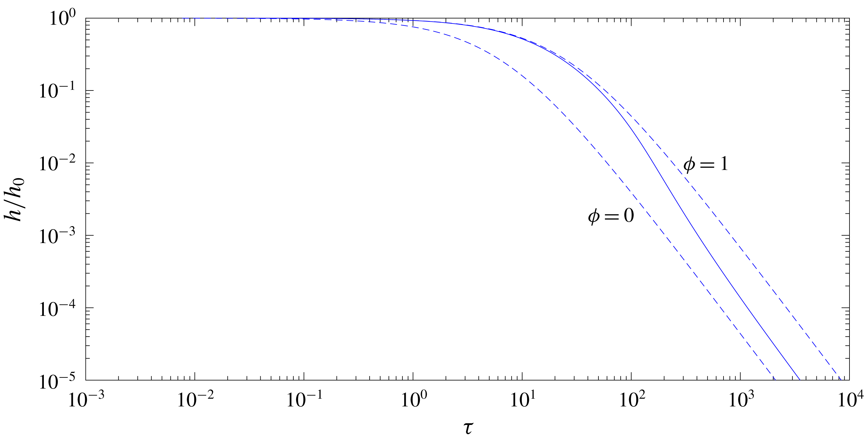
Figure 8. Same as figure 7, but for
 $\unicode[STIX]{x1D706}=0.1$
.
$\unicode[STIX]{x1D706}=0.1$
.
In figure 7 we show the time evolution of
 $h/h_{0}$
for
$h/h_{0}$
for
 $\unicode[STIX]{x1D719}=0.5$
and
$\unicode[STIX]{x1D719}=0.5$
and
 $\unicode[STIX]{x1D706}=1$
, obtained by solving (D 6) using (5.7). At sufficiently large times the scaled period
$\unicode[STIX]{x1D706}=1$
, obtained by solving (D 6) using (5.7). At sufficiently large times the scaled period
 $l$
becomes large whereby
$l$
becomes large whereby
 $F^{\bot }$
is approximately given by (5.11); the time variation of
$F^{\bot }$
is approximately given by (5.11); the time variation of
 $h/h_{0}$
thus approaches the power law (D 9). By that time,
$h/h_{0}$
thus approaches the power law (D 9). By that time,
 $h/h_{0}$
is of order
$h/h_{0}$
is of order
 $10^{-3}$
.
$10^{-3}$
.
More enlightening is the comparable evolution for the smaller period
 $\unicode[STIX]{x1D706}=0.1$
, described in figure 8. With
$\unicode[STIX]{x1D706}=0.1$
, described in figure 8. With
 $\unicode[STIX]{x1D706}$
being small,
$\unicode[STIX]{x1D706}$
being small,
 $F^{\bot }$
is approximately given by the small-
$F^{\bot }$
is approximately given by the small-
 $l$
approximation (5.11) for moderate
$l$
approximation (5.11) for moderate
 $h/h_{0}$
; the time evolution is accordingly identical to that of a cylinder approaching a homogeneous solid surface, namely (D 7). Only when
$h/h_{0}$
; the time evolution is accordingly identical to that of a cylinder approaching a homogeneous solid surface, namely (D 7). Only when
 $h/h_{0}$
becomes comparable to
$h/h_{0}$
becomes comparable to
 $\unicode[STIX]{x1D706}$
does the
$\unicode[STIX]{x1D706}$
does the
 $h^{-3/2}$
drag scaling break down and the time evolution ‘detaches’ from approximation (D 7). At sufficiently large times, the scaled period
$h^{-3/2}$
drag scaling break down and the time evolution ‘detaches’ from approximation (D 7). At sufficiently large times, the scaled period
 $l$
eventually becomes large and the time variation of
$l$
eventually becomes large and the time variation of
 $h/h_{0}$
approaches the power law (D 9). Corresponding to these trends we see that the curve representing the time variation of
$h/h_{0}$
approaches the power law (D 9). Corresponding to these trends we see that the curve representing the time variation of
 $h/h_{0}$
with
$h/h_{0}$
with
 $\unicode[STIX]{x1D70F}$
is initially concave, but eventually becomes convex. This is in contrast to the limits of solid and free surface, where the simple relations (D 7) and (D 8) necessitate that the curve is concave throughout on a log–log scale.
$\unicode[STIX]{x1D70F}$
is initially concave, but eventually becomes convex. This is in contrast to the limits of solid and free surface, where the simple relations (D 7) and (D 8) necessitate that the curve is concave throughout on a log–log scale.
Figure 8 suggests that, by the time asymptotic regime (D 9) is attained,
 $h/h_{0}$
is of order
$h/h_{0}$
is of order
 $10^{-5}$
. Practically speaking, this means that sedimentation over a small-periodicity surface (i.e. with the period being small compared to the initial clearance) will be affected by short-range (e.g. van der Waals) interactions with the surface long before the power law (D 9) is approached. Such sedimentation processes are hence crucially affected by the breakdown of the
$10^{-5}$
. Practically speaking, this means that sedimentation over a small-periodicity surface (i.e. with the period being small compared to the initial clearance) will be affected by short-range (e.g. van der Waals) interactions with the surface long before the power law (D 9) is approached. Such sedimentation processes are hence crucially affected by the breakdown of the
 $h^{-3/2}$
scaling law for the drag.
$h^{-3/2}$
scaling law for the drag.


