


Introduction
The spatial distribution and storage of soil organic carbon (SOC) represent the basic knowledge needed to understand soil hydrological properties and the cycling of global carbon, and play important roles in precision agricultural management (Six et al., Reference Six, Paustian, Elliott and Combrink2000; Lal, Reference Lal2003). Natural factors (e.g. soil parent material, climate, topography and vegetation) and human activities (e.g. land management, land use and degradation) can influence soil moisture, ventilation conditions and soil temperature, which can then collectively influence the decomposition and transformation of SOC via soil microbes. These environmental factors and such transformation processes may result in spatial instability and non-uniformity of SOC in different landscapes (Song et al., Reference Song, Brus, Liu, Li, Zhao, Yang and Zhang2016). Therefore, the current paper proposes a test methodology for accurate estimation of SOC stocks that extracts valuable information inherent in data on complex environmental factors.
The spatial analysis of soil distribution patterns is an important field in soil science. Adjacent soil patterns share similar natural environments and tillage methods. This condition results in the spatial dependence of SOC in nearby geographical locations. In addition, SOC has spatial heterogeneity because the environment varies with scale and geographical location (Mishra et al., Reference Mishra, Lal, Liu and Van Meirvenne2010). Natural and human-induced factors, which influence SOC content, interact and affect each other resulting in complex inter-relationships and multicollinearity. Multicollinearity generates data redundancy and contradicts the standard hypothesis regression model that explanatory variables should be independent from one another (Liu et al., Reference Liu, Wang, Yue and Hu2013; Conforti et al., Reference Conforti, Castrignano, Robustelli, Scarciglia, Stelluti and Buttafuoco2015). Therefore, multicollinearity among impact factors must be eliminated before constructing a SOC model (Kumar et al., Reference Kumar, Lal, Liu and Rafiq2013; Sun et al., Reference Sun, Zhu, Huang and Guo2015). The conventional method is to extract the valuable variables by Pearson's correlation coefficient, stepwise linear regression or analysis of variance, and then construct predictive models (Kumar et al., Reference Kumar, Lal and Liu2012a; Guo et al., Reference Guo, Zhao, Zhang, Chen, Linderman, Zhang and Liu2017). These methods ignore the valuable information from secondary environmental factors. Principal component analysis (PCA) is a widely used technique because it can decrease the basic dimensions of input parameters and reduce data redundancy (Song et al., Reference Song, Brus, Liu, Li, Zhao, Yang and Zhang2016). However, conventional PCA does not consider spatial relations and is not designed specifically to identify spatial structures.
Several prediction methods, ranging from simple regression models to geostatistical models, have been suggested for mapping the SOC density (SOCD) from sparse soil samples to continuous surfaces. In terms of geostatistical approaches, recent studies have been devoted to the utilization of a variety of environmental variables for enhanced SOCD modelling (Kumar et al., Reference Kumar, Lal and Lloyd2012b). Ordinary kriging (OK) is a method used commonly for estimating untested locations by calculating the weighted averages of explained variables from observed samples (Jobbágy and Jackson, Reference Jobbágy and Jackson2000). Specifically, when the correlated environmental variables are valuable, they can provide great help in constructing the prediction models of SOCD with high prediction accuracy and limited observations (Keser et al., Reference Keser, Duzgun and Aksoy2012). The ordinary co-kriging (OCK) model can be used to interpolate the spatial distribution of soil attributes based on the related and appropriate regionalized variables, if the main soil attribute is sparse but the related auxiliary information is abundant (Wang et al., Reference Wang, Zhang and Li2013b). As the representative of traditional regression models, ordinary least squares (OLS) can minimize the sum of the squared vertical distances between the predicted data and the observed data through linear approximation (Evrendilek et al., Reference Evrendilek, Celik and Kilic2004), and the relationships between the soil properties and environmental variables can be used to predict the soil properties in unknown geographical locations by OLS. However, traditional regression methods only use the available data at target locations and ignore existing spatial autocorrelation of SOCD and its auxiliary variables (Liu et al., Reference Liu, Guo, Jiang, Zhang and Chen2015). Geographically weighted regression (GWR) considers the spatial weights between the independent and dependent factors relative to traditional regression models (Harris et al., Reference Harris, Fotheringham, Crespo and Charlton2010). Also, the coefficients of the GWR model can respond to the spatial non-stationary characteristics of explanatory variables to the study object in geographical locations (Keser et al., Reference Keser, Duzgun and Aksoy2012; Wang et al., Reference Wang, Kang, Sun and Chen2013a).
Chahe Town, located in the middle of Jianghan Plain, China, was chosen as the study region. Jianghan Plain is an important agricultural region in China as it is a typical alluvial plain. In the current paper, PCA was performed to capture extensive explanatory variable information via orthogonal transformation. Two geostatistical approaches (OK and OCK) and two regression approaches (OLS and GWR) were used to estimate the spatial distribution of SOCD with the help of the principal components (PCs) which were processed via PCA. The aims of the current work are (1) to extract the valuable information from the complicated and various environmental factors by PCA method, (2) to construct a high-precision and efficient prediction models of SOCD, and (3) to draw the spatial distribution characteristics of SOCD by environmental factors.
Materials and methods
Study area
Chahe Town is located at the centre of Jianghan Plain, China (29.39–30.13° N, 113.6–114.05° E). The elevation ranges from 2 to 35 m asl, and the geographical area covers 153 km2. Jianghan Plain is a typical alluvial plain and it is an important agricultural region in China that provides cotton, commodity grains and edible oil. The mean annual precipitation is 1154 mm and the average air temperature is 16.1 °C. A total of 260 topsoil samples were collected in June 2013 by random sampling. However, the minimum distance between two soil samples was >100 m. The potassium dichromate method was used to measure soil organic matter (SOM) content (Viscarra Rossel and McBratney, Reference Viscarra Rossel and McBratney1998). The soil types are paddy soil, moisture soil, dark yellow-brown soil and yellow-brown soil based on the Chinese soil taxonomy classifications (Shi et al., Reference Shi, Yu, Warner, Sun, Petersen, Gong and Lin2006). The approximate classifications based on the World Reference Base of Soil Resources (Deckers et al., Reference Deckers, Nachtergaele and Spaargaren1998) are as follows: Typical Haplaquept, Dystrochrept, Eutroboralf and Hapludalf. The spatial distribution of the sampling sites is shown in Fig. 1.
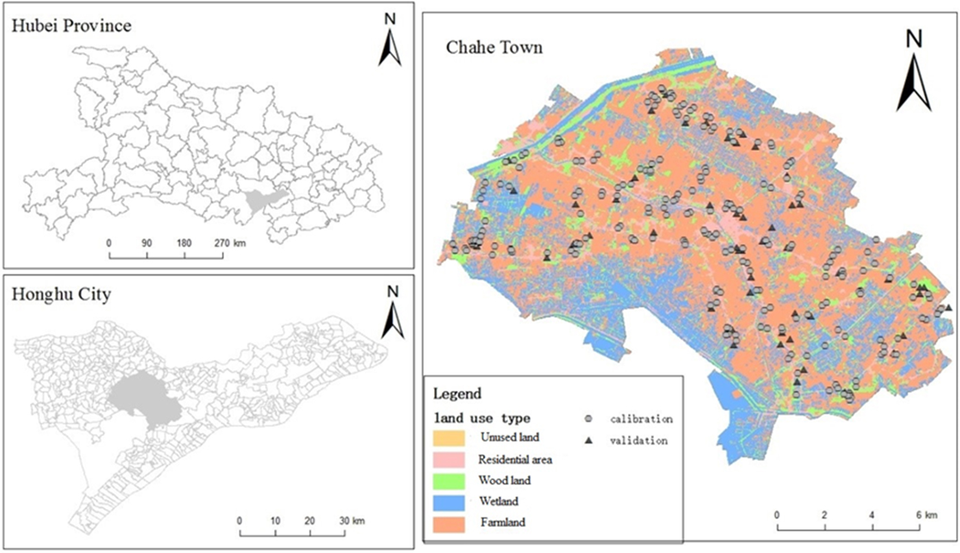
Fig. 1. Location of the study area in Chahe Town and the spatial distribution of samples for model calibration (n = 173) and validation (n = 87). Colour online.
The auxiliary variable data
The spatial distribution characteristics of SOC is affected by multitudinous environmental factors in different geographical locations. The terrain factors (e.g. elevation, slope and aspect), distance factors (e.g. nearest distance to construction area (TRA) and road (TRD)), and remote vegetation indices such as the normalized difference vegetation index (NDVI) and normalized difference moisture index (NDMI) were chosen as the auxiliary variables (Wilson and Sader, Reference Wilson and Sader2002). These were calculated as follows:
 $$\eqalign{& {\rm NDVI} = ({\rm NIR}-{\rm RED})/({\rm NIR} + {\rm RED}) \cr & {\rm NDMI} = ({\rm NIR}-{\rm MIR})/({\rm NIR} + {\rm MIR})} $$
where NIR denotes the near-infrared band, RED denotes the red band and MIR denotes the middle-infrared band of the Landsat 8 OLI imagery. The elevation, slope and aspect were calculated with the Global Digital Elevation Model Version 2 using ArcGIS 10.3 (ESRI Inc., Redlands, CA, USA), and the Euclidean distance tool of ArcGIS was used to calculate TRD and TRA. Aspect is expressed in positive degrees from 0 to 359.9, measured clockwise from north. If the input raster is flat with zero slope, the aspect is assigned −1. The land use types in the study region were classified by Landsat 8 OLI image on 26 June 2013 with 30 m spatial resolution. The atmospheric rectification and geometric rectification of the OLI images were first processed by ENVI 4.6 (ITT, Boulder, CO, USA). The NDVI and NDMI were calculated based on this remote-sensing image. Subsequently, land use types were interpreted by man–machine collaboration based on the OLI images, and the woodland, farmland, residential area (construction area), wetland and unused land were classified according to the Chinese Academy of Sciences (Wang et al., Reference Wang, Liu, Zhang, Zhou and Zhao2001). Finally, a field survey was applied to improve the interpretation accuracy until it was >80%. The TRA and TRD were calculated based on this interpretation result. The land use types were thereafter quantified with the land use degree comprehensive index (LDCI). The equation is as follows:
 $${\rm LDC}{\rm I}_a = 100 \times \mathop \sum \limits_{i = 1}^n A_i \times C_i$$
Where LDCIa is the land use degree index; A i is the land use classification index and the quantitative values are 4, 3, 2, 2 and 1 for construction area, farmland, woodland, wetland and unused land; and C i is the area percentage of different land use types in one unit. High A i values indicate a large effect of human activities at one region (Zhuang and Liu, Reference Zhuang and Liu1997). The LDCI has been used as the auxiliary variable in predicting SOCD and it has been proved that LDCI has significant correlation with SOCD (Liu et al., Reference Liu, Guo, Jiang, Zhang and Chen2015).
Coefficient of variation
The coefficient of variation (CV) shows the dispersion degree of data sets and is defined as the ratio of the standard deviation value to the mean value. High CV values indicate a high degree of variation for a particular variable. The variability of variable is classified based on the research of Wilding (Reference Wilding, Nielsen and Bouma1985), where properties with CV < 0.15 are least variable, properties with 0.15 < CV < 0.35 are moderately variable and those with CV > 0.35 are most variable.
Calculation of soil organic carbon density
Soil organic carbon density is calculated as follows:
 $$\rho _{{\rm SOC}} = \mathop \sum \limits_{i = 1}^n (1-\theta _i\% ) \times p_i \times C_i \times T_i/100\; $$
where ρ soc is SOCD (kg/m2) of the top soil (0–20 cm), i is the soil horizon, θ i% is the gravel concentration (>2 mm) in the ith horizon, p i is the soil bulk density in the ith horizon (g/cm3), C i is SOC content (g/kg) obtained by multiplying SOM by 0.58 (Bemmelen conversion fraction) and T i is the soil thickness (cm) in the current study.
Model calibration
Topsoil samples (260) were divided into a calibration data set (n = 173, 2/3) and validation data set (n = 87, 1/3) on the basis of the Kennard–Stone algorithm (De Groot et al., Reference De Groot, Postma, Melssen and Buydens1999). Eight environmental factors (TRA, TRD, NDMI, NDVI, elevation, slope, aspect and LDCI) were used as auxiliary variables. Principal component analysis was performed as the pre-processing method to reduce the multicollinearity and the dimension of these variables. A suitable number of PCs were chosen as the explanatory variables for constructing the prediction models of SOCD via OK, OCK, OLS and GWR.
Principal component analysis
Principal component analysis, a widely used traditional statistical procedure, can explore trends in multiple variables. The procedure transforms correlated variables into the number of independent variables which are uncorrelated, namely, PCs, which are linear combinations of the original variables. The first principal component (PC1) includes the largest possible variance, under the constraint that the preceding component is orthogonal, and each subsequent component has the highest possible variance in turn (Jeyabharathi and Suruliandi, Reference Jeyabharathi and Suruliandi2013). Other details on PCA are found in the work of Johnson and Wichern (Reference Johnson and Wichern2002), which provides a good overview of PCA.
Ordinary kriging and ordinary co-kriging
Kriging as an advanced geostatistical procedure can generate a continuous surface from sparse soil samples based on their attributes. Assume Z(Xi) is a regionalized variable with a variogram γ(h), which is a function describing the spatial aggregation field or stochastic process Z(u). Exponential and spherical methods are used as the semi-variance model of the variation function. The spherical function is defined as:
 $$\gamma \lpar h \rpar = \left\{ {\matrix{ 0 \hfill & {h = 0} \hfill \cr {C_0 + C\left( {\displaystyle{{3h} \over {2h}}-\displaystyle{{h^3} \over {a^3}}\;} \right)} \hfill & {0 \lt h \le a} \hfill \cr {C_0} \hfill & {h \gt a} \hfill \cr}} \right.$$
The function of a Gaussian model can be estimated as follows:
 $$\gamma (h) = \left\{ {\matrix{ 0 & {h = 0} \cr {C_0 + C(1-{\rm e}^{-(r^2/a^2)}\; )} & {h \gt 0} \cr}} \right.$$
In these two equations, a is the range of the soil samples; h is the spatial lag; C 0 is the nugget; and C 0 + C is the partial sill.
The traditional OK can provide unbiased estimates with minimum errors. The function of OK is expressed as
 $$Z^{^\ast}(x_0) = \mathop \sum \limits_{i = 1}^n \lambda _i(x_0)Z(x_i)$$
Here,  $\sum\nolimits_{i = 1}^n {\lambda _i(x_0) = 1} $; Z*(x 0) is the predicted value of the variable z at location x 0; Z(x i)is the measured data; λ i(x 0) refers to the weights associated with the measured values; and n is the number of predicted values within some neighbour soil samples.
Ordinary co-kriging is used to incorporate an auxiliary variable in process and is usually used in cases when two or more auxiliary variables are exhaustively available. The OCK estimator is written as follows:
 $$\eqalign{Z_{{\rm OCK}}^{^\ast} (u) = \mathop \sum \limits_{\alpha _1 = 1}^{n_1(u)} \lambda _{\alpha _1}^{{\rm ock}} (u)Z_1(u_{\alpha _1}) + \mathop \sum \limits_{i = 2}^{N_v} \lambda _i^{{\rm ock}} (u)[Z_i(u)-m_i + m_1]}\; $$
where the single constraint is that the sum of all weights must be equal to 1.
 $$\mathop \sum \limits_{\alpha _1 = 1}^{n_1(u)} \lambda _{\alpha _1}^{{\rm ock}} (u) + \mathop \sum \limits_{i = 2}^{N_v} \lambda _i^{{\rm ock}} (u) = 1\; $$
where,  $Z_{{\rm OCK}}^* (u)$ is the predicted value of the original variable Z 1 at unknown location u;
  $\lambda _i^{{\rm ock}} (u)$ is the weight of measured values in different geographical locations;
  $Z_1(u_{\alpha _1})$ denotes the primary values; N v is the total number of auxiliary variables;
  $Z_1(u_{\alpha _1})$ is the correlate data of the ith auxiliary variable;
  $\lambda _i^{{\rm ock}} (u)$ is the weight of the correlate data of the ith variable; and m 1 is the mean of the primary variables and m i is the mean of the ith auxiliary variable.
Geographically weighted regression model
An extension of the traditional regression model, GWR considers the geographical locations and spatial weights of auxiliary variables (Brunsdon et al., Reference Brunsdon, Fotheringham and Charlton1998; Fotheringham et al., Reference Fotheringham, Brunsdon and Charlton2002). It is calculated as follows:
 $$\hat{C}_{{\rm gwr}}(s_0) = \beta _0 + \mathop \sum \limits_{k = 0}^p \beta _k(s_0) \times X_k(s_0) + \varepsilon (u)\; $$
where  $\hat{C}_{{\rm gwr}}(s_0)$ represents the predicted value of SOCD at the location of S0; X k(s 0) is the independent variables at the geographical location of S 0; β 0 means the intercept; β k(s 0) is the coefficient of GWR which considers the relationship between the SOCD and the auxiliary variables; p is the number of the soil samples; and ε (u) is the error term.
The corrected Akaike information criterion (AICc) was used to determine the optimal bandwidth in the current paper. The AICc is defined as:
 $${\rm AICc} = -2\ln L(\hat{\theta} _{\rm L},X) + 2q$$
where  $\hat{\theta} _{\rm L}$ is the maximum likelihood estimator, and q is the number of unknown parameters. A high likelihood function indicates an accurate estimator. Thus, a minimum value of AICc is suitable to optimize the model.
Model evaluation
Four SOCD models were constructed using calibration data sets based on OK, OCK, OLS and GWR. The predicted accuracy of different models is evaluated by the mean absolute estimation error (MAEE), root mean square error (RMSE) and Pearson's correlation coefficient (r) in validation data sets.
 $${\rm MAEE} = \displaystyle{1 \over n}\mathop \sum \limits_{i = 1}^n \vert {x_i-y_i} \vert \; $$
 $${\rm RMSE} = \sqrt {\displaystyle{1 \over n}\mathop \sum \limits_{i = 1}^n {(x_i-y_i)}^2} \; $$
 $$r = \displaystyle{{n\mathop \sum x_iy_i - \mathop \sum x_i\mathop \sum y_i} \over {\sqrt {n\mathop \sum x_i^2 -{\left( {\mathop \sum x_i} \right)}^2} \sqrt {n\mathop \sum y_i^2 -{\left( {\mathop \sum y_i} \right)}^2}}}$$
where x i is the estimated SOCD at location i, y i is the observed SOCD at geographical location i, and n is the number of sample observations. An accurate model should have the lowest RMSE and MAEE values.
Results
Descriptive statistics
The statistical summary of SOCD and environmental factors is shown in Fig. 2. The observed SOCD varied from 0.33 to 11.23 kg/m2, with an arithmetic mean of 5.05 kg/m2 and a range of 10.91 kg/m2. The values of skewness and kurtosis were 0.39 and 3.62, respectively, which implied that the samples fitted a normal distribution. Thus, the original SOCD data can be used to construct spatial models without any transformation. The CV of SOCD was 32.50%, which indicated that SOCD in the study region was moderately variable. For the other environmental variables, elevation had the least variability; NDVI, NDMI and LDCI were moderately variable; and all the other variables were highly variable. The mean values of TRA, TRD, NDMI, NDVI, elevation, slope, aspect and LDCI were 176.64 m, 813.15 m, 0.27, 0.41, 21.59 m, 1.25°, 109.41 and 2.57, respectively. The topography of the study area is flat, with slope ranging from 0 to 6.75°. The LDCI ranged between 1 and 3.46 (mean 2.57). The values of NDVI were from 0.06 to 0.58, which showed that most of the land surface was covered with vegetation. Figure 2 also shows the basic statistics of other environmental variables.

Fig. 2. Descriptive statistics of measured soil organic carbon density and other environmental variables of the study area (n = 260). SOCD, soil organic carbon density; NDVI, normalized difference vegetation index; NDMI, normalized difference moisture index; TRD, recent distance to road; TRA, recent distance to city; CV, coefficient of variation; LDCI, land use degree comprehensive index.
The formation, decomposition and transformation of SOC were influenced by many environmental factors, which were complex and varied greatly across different natural landscapes (Zhi et al., Reference Zhi, Jing, Zhang, Wu, Ni, Chen and Xu2013). The degree of influence of these factors on SOCD should be distinguished and decided. Principal component analysis was used to classify these factors into several categories and to eliminate data redundancy. The major information of the impact factors was captured by PCA (Table 1). The first three PCs were chosen as the explanatory variables, as their eigenvalues were >1, thus explaining 60% of the observed variance in the environmental factors. The first component (PC1) explained approximately 26.7% of the total variance and had a significant positive correlation with NDMI (0.90) and NDVI (0.93). Both are spectral indices calculated with the spectrum of remote-sensing images and reflected soil moisture and vegetation growth. The second component (PC2) explained about 18.0% of the observed variance in the data set. This component was correlated negatively with TRA (−0.44) and TRD (−0.68) but positively with elevation (0.72) and LDCI (0.44). It was the summary of the elevation and human-induced factors. The third component (PC3) accounted for an additional 15.5% of the observed variance in the data set and had a strong positive correlation with aspect (0.70) and slope (0.80): it represented terrain information. The relationships observed from the PCA suggested that various environmental factors were intricately connected in the study region.
Table 1. Eigenvalues and the eigenvectors of the correlation matrix in principal component analysis

NDVI, normalized difference vegetation index; NDMI, normalized difference moisture index; TRD, recent distance to road; TRA, recent distance to city; LDCI, land use degree comprehensive index; PC, principal component.
Figure 3 shows the spatial distribution characteristics of the first three PCs, which represent different environmental factors according to the eigenvectors of the correlation matrix. PC1, which represented vegetation growth and soil moisture, was related positively to NDVI and NDMI (Table 1). The PC1 value ranged from −5.76 to 3.14, with large values indicating high ratios of vegetation and soil moisture. High PC1 values were observed in the southwest of the study area, where many farmland area and woodland could be found. Low PC1 values were observed in the south, where wetland was the main land use type. PC2 represented the elevation and human-induced factors. PC2 was negatively related to TRA and TRD but was positively related to elevation and LDCI (Table 1). PC2 also showed some zonal characteristics because of the influence from the road and residential area. Thus, the PC2 values were the comprehensive results of elevation, TRA, TRD and LDCI, and human activities were the main influence factors on PC2. Low PC2 values were observed at the middle of the study area where residential area is the main land use type. High PC2 values were found at the edge of the study area, which was located far away from areas with human activities. PC3 represented terrain information because of its positive relationship with slope and aspect (Table 1). High PC3 values indicated high slopes and the proximity of a specific region to the south of the aspect. Although the impact factors were transformed by PCA, these three PCs could reflect the original information of these factors according to the eigenvectors of the correlation matrix. The values of the PCs in different geographical locations could be interpreted on the basis of natural or human-induced factors: PC1 representing the remote-sensing vegetation index, PC2 representing the human activities and PC3 representing the topographic features.

Fig. 3. Spatial distribution of the principal component scores: (a) first principal component scores (26.697%), (b) second principal component scores (18.026%) and (c) third principal component scores (15.507%). Colour online.
Diagnostic information of the geostatistical and regression models
Geostatistical models (OK and OCK) and regression models (OLS and GWR) were used to simulate SOCD in the study region. Table 2 shows the diagnostic parameters for the calibration data set. The major ranges of the empirical semi-variable function were 194.0 and 493.2 m. They were used in the fitting procedure, which involved modelling with OK and OCK approaches. The ratio of C 0/(C 0 + C) reflects the spatial structure of the estimated factors, with 0–25% indicating strongly structured spatial dependence, 25–75% indicating moderate dependence and >75% indicating weak dependence (Jobbágy and Jackson, Reference Jobbágy and Jackson2000). The ratio for SOCD in OK was 11.1%, which indicated the strong dependence of SOCD. By contrast, the ratio for SOCD in OCK was 61.7%, which indicated the moderate dependence of SOCD. Such a difference can be attributed mainly to the fact OCK considered the PCs as auxiliary variables and that part of the spatial distribution of SOCD was influenced by their spatial characteristics. The effective number (8.3) and sigma (0.48) of GWR are important parameters in GWR model, and these figures are always used to choose the suitable bandwidth. The AICc of GWR was 307.34, which was smaller than that of OLS (309.5) and indicated that GWR has better simulation precision than OLS. The RMSE can be used to evaluate simulation precision between different models. In the current study, the regression models yielded better results than the geostatistical models in terms of RMSE values, and also the spatial characteristics and the auxiliary variables played an important role in improving the model performance.
Table 2. Diagnostic parameters of the geostatistical and regression models

SOCD, soil organic carbon density; OK, ordinary kriging; OCK, ordinary co-kriging; OLS, ordinary least squares; GWR, geographically weighted regression; C 0, nugget; C, partial sill; C 0 + C: total sill; RMSE, root mean square error; Range, major range of the empirical semi-variable function, the range of exponential is 3a and the range of Gaussian is  $\sqrt 3 a$; AICc, corrected Akaike information criterion.
RMSE, MAEE and r were used to evaluate the performance of these four models based on the validation data set, namely, OK, OCK, OLS and GWR. The RMSE values of these models were 1.2, 1.1, 1.2 and 1.1 kg/m2; MAEE values were 0.91, 0.92, 0.93 and 0.85 kg/m2; and r values were 0.30, 0.39, 0.35 and 0.46. The RMSE v. the MAEE points are plotted in Fig. 4 for a comprehensive comparison of the model performance. As shown in Fig. 4, a long distance from the point to the origin would result in poor prediction accuracy. The distances of the OK, OCK, OLS and GWR models were 1.50, 1.46, 1.49 and 1.39, respectively. The highest prediction accuracy was seen in GWR, followed by OCK, OLS and OK. In these models, OLS only considers relationships between the auxiliary variables and SOCD, and OK only considers the spatial characteristics of SOCD. Moreover, GWR could account for both the spatial trend and local variations of the relationships between the environmental factors and SOCD, whereas OCK could not easily capture the valuable information regarding environmental factors in unknown soil samples. Thus, environmental factors and local spatial variation of SOCD played important roles in predicting SOCD, and GWR is a very promising spatial interpolation method for predicting soil properties.

Fig. 4. Root mean square error (RMSE) v. mean absolute estimation error (MAEE) plots for the four models and their Pearson's r values, namely, ordinary kriging (OK), ordinary co-kriging (OCK), ordinary least squares (OLS) and geographically weighted regression (GWR). Colour online.
Analysing the spatial distribution of soil organic carbon density
Figure 5 illustrates the spatial distribution maps of SOCD estimated by OK, OCK, OLS and GWR. Generally, the spatial distribution characteristics of SOCD are the same across the four images. Low estimated values of SOCD were concentrated in the middle region and high estimated values were distributed at the edge of the study region. Between these two kinds of models, the SOCD values ranged from 0.32 to 11.23 kg/m2 in the geostatistical models and from 2.76 to 9.97 kg/m2 in the regression models. The geostatistical models had the bigger numerical ranges than the regression models because the extremums of SOCD were smoothed by the regression models. Meanwhile, in the middle area, the area of low (0.33–4.98 kg/m2) SOCD values in geostatistical models were bigger than regression models. The spatial distribution of SOCD under these two kinds of models obviously differed. The shape was similar to the rings in geostatistical models, but the lines were similar to those in the regression models. These results can be attributed to the fact that geostatistical models are spatial interpolation models and that regression models are multiple linear regression models. The measured SOCD and environmental variables played different roles in estimating SOCD from different models.
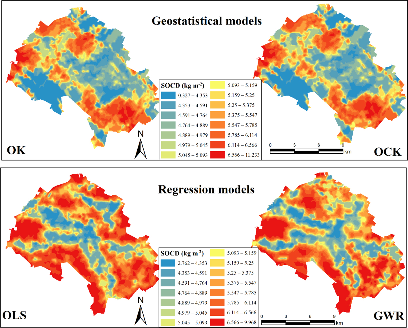
Fig. 5. Spatial distribution of soil organic carbon density (SOCD) by ordinary kriging (OK), ordinary co-kriging (OCK), ordinary least squares (OLS) and geographically weighted regression (GWR). Colour online.
Although these two models shared many similarities, their interiors revealed detailed differences. Relative to OK, the spatial distribution of SOCD in OCK can reflect more detailed information in the local spatial, and the different values of SOCD were divided more accurately. This phenomenon resulted from the fact that OK only considered the spatial variation and dependency of SOCD, whereas OCK considered the spatial information of environmental factors that influenced the spatial distribution of SOCD. In Fig. 5, the spatial distribution features of SOCD were similar between OLS and GWR. High values were found in the west and the northeast portion of the study region, and low values were concentrated in the middle part of the study area. The spatial patterns of SOCD were different in many patches because the values of SOCD were estimated through auxiliary variables and their weights. Table 3 shows the global coefficients and the important parameters of PCs in the OLS model, while Fig. 6 presents the local coefficients of PCs in different locations in GWR model. The spatial weights of the auxiliary variables were constant in different geographical locations in the OLS model but were different in the GWR model.
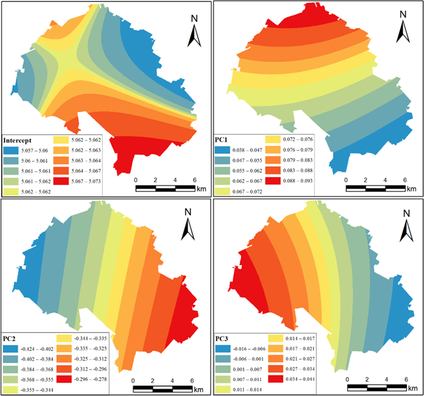
Fig. 6. Spatial distribution of the coefficients of different auxiliary variables in the geographically weighted regression (GWR) model. Colour online.
Table 3. Principal component variables in the ordinary least squared (OLS) model

s.e., standard error of mean; VIF, variance inflation factor.
Discussion
Influence of different independent variables on soil organic carbon density
Soil organic carbon density is influenced by different environmental variables, and such influence results in strong spatial heterogeneity and spatial dependence; these variables vary with the environment and geographical locations (Zhan et al., Reference Zhan, Cao, Han, Huang, Tu, Ping and An2013). Kumar et al. (Reference Kumar, Lal and Liu2012a) integrated natural variables (e.g. temperature, precipitation, elevation, slope, geology and NDVI) with human variables (e.g. land use) in their spatial modelling of SOCD in the state of Pennsylvania, USA. Zhang et al. (Reference Zhang, Tang, Xu and Kiely2011) investigated and used environmental factors (e.g. rainfall, land cover and soil types) as explanatory variables to establish SOC models. Therefore, the influence of different environmental variables and human activities should be explored when mapping SOCD. The constant of a regression model can guarantee that the residuals have a zero mean. PC1 had a coefficient of 0.06 in the OLS model but a coefficient of 0.04–0.09 in the GWR model. PC1 was also positively correlated with SOCD and high PC1 values equate to high SOCD. This result is reasonable because PC1 was representative of NDVI and NDMI, which were usually positively related to SOCD (Ruiz-Colmenero et al., Reference Ruiz-Colmenero, Bienes, Eldridge and Marques2013). PC1 had a stronger influence in the north than in the south, possibly because of the differences in land use types, soil moisture and land cover. Normalized difference moisture index was an indicator of soil moisture, and a higher soil moisture could improve the living environment of soil microbes, accelerate the transformation and decomposition of SOC, and prevent the net loss of organic soils from oxidation (Liu et al., Reference Liu, Guo, Jiang, Zhang and Chen2015). PC2 had a coefficient of −0.35 in OLS model and a coefficient of −0.02 to −0.28 in GWR model. PC2, which represented elevation and human-induced factors, had a negative correlation with SOCD. On the basis of the eigenvectors and coefficients of the models, SOCD had a positive correlation with TRA and TRD but a negative correlation with elevation and LDCI. Soil organic carbon density decreased along with an increase in elevation because the soil could be easily transferred from highly elevated areas to low elevated areas by rains or winds. Moreover, SOC tends to accumulate in low-lying areas (Liu et al., Reference Liu, Guo, Jiang, Zhang and Chen2015). The LDCI is a comprehensive index that indicates the influence of human activities on land use. A strong influence of human activities would result in a low SOCD value because human activities could destroy the soil structure that provides a favourable living environment for soil microbes (Wu et al., Reference Wu, Guo and Peng2003). The coefficients of TRA and TRD reflected the influence of the residential area and road on SOCD. A short distance would result in a low SOCD because closeness to residential areas and roads would strengthen the influence of human disturbance on SOCD. The vegetation and soil structure in natural landscapes are usually destroyed during the processes of urban development and road construction, thereby accelerating soil erosion, reducing soil nutrients and eventually reducing SOCD (Shubin, Reference Shubin2006). PC3 had a coefficient of 0.01 in the OLS model and a coefficient of −0.02 to 0.04 in the GWR model. The relationships between the PC3 and the slope and aspect were positive, which means SOCD was positively related to the slope and aspect, except in a small area in the southeast. Slope could influence the accumulation of soil, while aspect could influence the time exposure of sunlight, which would subsequently influence soil moisture and the activities of soil microbes (Yimer et al., Reference Yimer, Ledin and Abdelkadir2006). In summary, the coefficient maps of GWR can reflect the influence of different explanatory variables on SOCD across regions. This finding could help environmentalists distinguish the importance of different impact factors and help farmers manage their farmlands in a suitable and scientific way.
Evaluating the prediction accuracy of the ordinary kriging, ordinary co-kriging, ordinary least squares and geographically weighted regression models
Previous studies have investigated a number of different estimation approaches considered here. For example, Zhang et al. (Reference Zhang, Tang, Xu and Kiely2011) evaluated the prediction accuracies of GWR, OK, inverse distance weighted and OLS in mapping SOC in Ireland by using rainfall, land cover and soil types as the explanatory variables. Wang et al. (Reference Wang, Zhang and Li2013b) used GWR and OCK to estimate the total nitrogen in soil by referring to elevation, slope, land use type, topographic wetness index and soil type. Kumar et al. (Reference Kumar, Lal, Liu and Rafiq2013) compared the application of GWR and OLS in mapping the spatial distribution of SOCD in Ohio, USA. These studies showed the potential of GWR in predicting soil properties by using its excellent prediction accuracy and various weight coefficient maps. However, these studies considered all environmental variables as explanatory variables and ignored the multicollinearity and redundancy among them. In the current paper, PCA was used as a pre-processing method in the present work to address the aforementioned problems and constructed prediction models according to the PCs of the selected environmental variables. The prediction accuracy of GWR was the highest among all the tested models (OCK, GWR, OLS and OK) for the auxiliary variables and the spatial weights estimated were found to be highly beneficial in predicting SOCD. Ordinary least squares achieved poor accuracy because this model ignored the spatial characteristics of both SOCD and the auxiliary variables (PC1, PC2 and PC3) and simply used PCs as explanatory variables to construct SOCD models. Moreover, OLS could not account for the spatially varying relationships between the environmental factors and SOCD. Ordinary kriging also obtained a low accuracy because this model only considered the spatial dependence of SOCD but ignored the valuable information from the environmental variables. Therefore, OK and OLS achieved lower prediction accuracies than the other two models. Both GWR and OCK utilized the spatial correlations of the environmental variables and SOCD during the model construction, but the auxiliary variables of the soil samples cannot be used to predict SOCD at unknown geographical locations by OCK. Geographically weighted regression can construct a soil SOCD map based on the relationship between the SOCD and the auxiliary variables, and this is why the GWR has better prediction accuracy than OCK. Meanwhile, the SOCD map that was interpolated with GWR could provide additional information on SOCD within local regions. The coefficient maps could reflect the influence degree of environmental variables to SOCD in different geographical locations. Thus, PCA is one useful method in reducing the dimensionality and redundancy of the auxiliary variables. Geographically weighted regression has enormous potential in enabling prediction of soil properties as it provides more information in explaining the local spatial relationships between the environment variables and SOCD.
Conclusion
A total of 260 soil samples from Chahe Town, which is located at the centre of Jianghan Plain, were analysed. Eight environmental variables (TRA, TRD, NDMI, NDVI, elevation, slope, aspect and land use type) were used as auxiliary variables to construct the prediction models of SOCD. The PCA method was used to reduce multicollinearity and redundancy of these environmental variables. The first three PC variables were chosen as explanatory variables. Two geostatistical models (OK and OCK) and two regression models (OLS and GWR) were used to map SOCD. As revealed by the evaluation indices (MAEE, RMSE and Pearson's r), GWR demonstrated the highest accuracy, followed by OCK, OLS and OK. The main reason was that GWR can capture more details on the local variation in SOCD and reflect the effects of auxiliary variables on SOCD. Therefore, the combination of PCA and GWR is a promising method in reducing the redundancy of environmental factors and in constructing prediction models of SOC stocks.
Financial support
This study was supported by the Natural Science Foundation of Hubei (2018CFB372); the Fundamental Research Funds for the Central Universities (2662016QD032); the Key laboratory of aquatic plants and watershed ecology of Chinese academy of sciences (Y852721s04), the Chinese National Natural Science Foundation (41371227); and the National Undergraduate Innovation and Entrepreneurship Training Program (201810504023, 201810504030).
Conflict of interest
None.
Ethical standards
Not applicable.


