


1. Introduction
Periodic submerged structures, either natural (such as tidally or wave generated small sandbars) or artificial (i.e. engineering structures), are often found in coastal areas. These support highly resonant free surface motions close to the structures if certain conditions are met. At these conditions, small reflected waves from successive structures, and the incident waves are in phase and add up to form a strong reflection (i.e. large free surface motions) at the seaward side. This resembles a classical phenomenon of ‘Bragg reflection’ in X-ray diffraction by crystalline materials, hence, the same terminology has also been widely used in the field of water waves. The conditions are then denoted ‘Bragg resonance conditions.’ The resonance may be excited in a linear or nonlinear fashion, and is of importance for coastal protection and sediment transport/dune growth in coastal areas (Heathershaw Reference Heathershaw1982).
Obviously, the dephasing (i.e. zero phases) between many reflected waves (from each member structure) and the incident wave is the critical action for Bragg resonance to manifest. Davies (Reference Davies1982a,Reference Daviesb) has demonstrated from his linear perturbation calculations that this zero-phase condition would be met if the ratio of surface and bottom wavelengths equals two (both surface waves and bottom structure are assumed to vary sinusoidally). The theory has been confirmed by experimental studies carried out by Heathershaw (Reference Heathershaw1982) and Davies & Heathershaw (Reference Davies and Heathershaw1984). Later, the generalized Bragg resonance conditions were proposed by Liu & Yue (Reference Liu and Yue1998), who treated the periodic bottom sinusoidal structure as artificial surface waves that have corresponding wavenumbers but zero frequencies. The criterion of wave resonance (i.e. linear combinations of wavenumbers/frequencies of each surface wave component equal zero) devised by Phillips (Reference Phillips1960) is then applicable for the problem of Bragg resonance involving bottom undulations. The aforementioned Bragg resonance condition in Davies (Reference Davies1982a,Reference Daviesb) that involves one bottom and two surface wave components is also represented and is denoted the class I Bragg resonance condition (Liu & Yue Reference Liu and Yue1998) or primary Bragg resonance condition (Yu & Howard Reference Yu and Howard2010).
It is well established that linear theory (with appropriate corrections for resonance conditions, and either solved analytically or numerically) can predict class I Bragg resonant waves with a reasonable level of accuracy (see e.g. Mei Reference Mei1985; Davies, Guazzelli & Belzons Reference Davies, Guazzelli and Belzons1989; Chamberlain & Porter Reference Chamberlain and Porter1995; Porter & Porter Reference Porter and Porter2003; Liu & Zhou Reference Liu and Zhou2014), although various nonlinear numerical simulations are also widely used. The latter, including a higher-order spectral (HOS) method (Liu & Yue Reference Liu and Yue1998), a fully nonlinear Boussinesq model (Gao et al. Reference Gao, Ma, Dong, Chen, Liu and Zang2021) and Navier–Stokes solver models (Huang & Dong Reference Huang and Dong2002; Hsu et al. Reference Hsu, Lin, Hsiao, Ou, Babanin and Wu2014), have the potential to capture possible nonlinearities involved. These theoretical and numerical studies as well as laboratory experiments (e.g. Heathershaw Reference Heathershaw1982; Davies & Heathershaw Reference Davies and Heathershaw1984) have shown that, in certain circumstances, very few small structures can reflect the incident wave energy substantially, and could then be an effective measure for shore protection. Thus, the concept of a Bragg breakwater, consisting of several periodic small bars, has been proposed by Mei, Hara & Naciri (Reference Mei, Hara and Naciri1988) as an alternative to a single massive breakwater on a weak seabed.
Bragg scattering has been crucial in the above work but largely focused on linear wave–wave and wave–structure interactions (that is, the superposition of linear incident and diffracted waves). For larger surface and/or bottom wave steepness, higher-order/nonlinear Bragg resonances resulting from nonlinear interactions among surface and bottom wave components are expected. Mattioli (Reference Mattioli1990) demonstrated that, for particular combinations of two sinusoidal bottom wave components, the response curve shows reflection peaks at distinct frequencies of class I Bragg reflection. This feature can be well explained by the generalized Bragg resonance conditions proposed by Liu & Yue (Reference Liu and Yue1998) mentioned above. It involves two surface and two bottom wave components; hence, it is denoted class II Bragg resonance, which manifests bottom nonlinearity.
In contrast, the resonance arising from free surface wave nonlinearity is denoted class III Bragg resonance. This would occur if the interaction between surface waves (with two different wavenumbers) and a periodic submerged structure (with a single wavenumber) gives rise to new waves with the wavenumber being equal to the difference or sum of those of the surface and the sinusoidal bottom waves. The former (the difference of the wavenumbers) travels away from the seaward side of the periodic structure (i.e. higher-order reflected waves, and a so-called sub-harmonic Bragg resonant wave), and the latter (the sum of the wavenumbers) away from the leeward side (i.e. higher-order transmitted waves, and a so-called super-harmonic Bragg resonant wave). That is, resonant interactions among one bottom and three surface waves are incurred in class III Bragg resonances, as suggested by Liu & Yue (Reference Liu and Yue1998).
Class III Bragg resonance (both sub- and super-harmonic) has been captured numerically by Liu & Yue (Reference Liu and Yue1998) using a HOS model, while the experimental evidence was provided by Peng et al. (Reference Peng, Tao, Liu, Zheng, Zhang and Wang2019). These (numerical and physical) experiments were carried out with carefully generated water waves over a sinusoidal bottom of carefully selected dimensions, informed by the aforementioned Bragg resonance conditions. That is, class I as well as class III sub- and super-harmonic Bragg resonances were observed separately with different bottom configurations (characterized by the bottom amplitude and wavelength). In addition, the relationship between the main characteristics of class III Bragg resonance (in terms of the resonant wave intensity and the resonance condition etc.) and the surface/bottom waves is still under-explored.
In this work, nonlinear Bragg resonances are investigated using two-dimensional (2-D) fully nonlinear numerical wave tanks (NWTs) solving the Poisson equation and the fully nonlinear free surface boundary conditions based on a higher-order boundary element method (HOBEM). The scenario considered is a 2-D surface wave propagating towards and over a parallel periodic sinusoidal structure (also known as a wavy bottom, and the member structures are denoted ripples hereafter) with a single wavenumber. Even for this rather simpler situation, the importance and implication of the nonlinear resonances should be emphasized; multiple Bragg resonances may occur for the same system/bottom topology. In addition to Bragg resonance conditions (i.e. classes I and III) mentioned above, resonances at a surface wavenumber close to an integer multiple of half a bottom wavenumber (the integer could be larger than 1) may occur (Yu & Howard Reference Yu and Howard2010). The improved understanding of the influence of the incident wave and bottom sinusoidal structure on class III Bragg resonance is also of interest in this work. This also helps to provide guidance/knowledge in designing the Bragg breakwater, as first proposed by Mei (Reference Mei1985).
2. Re-creating published benchmarking experiments
In this section, experimental and numerical details of primary importance are presented; more complete information describing the experiments on class III Bragg resonance can be found in Peng et al. (Reference Peng, Tao, Liu, Zheng, Zhang and Wang2019), and the NWT employed in Appendix A and in Ning et al. (Reference Ning, Chen, Zhao and Teng2016). The verification of class I Bragg resonance has also been carried out, but is omitted here for brevity. Class III Bragg resonance covers both linear and nonlinear interactions between the surface and bottom waves; the former is essential for class I Bragg resonance to be effectuated, as mentioned previously.
2.1. Experimental
The experiments of Peng et al. (Reference Peng, Tao, Liu, Zheng, Zhang and Wang2019) were carried out in a 2-D wave flume in which 2-D plane surface waves were generated and propagated over parallel bottom ripples of sinusoidal shape. The parameters of the surface and bottom waves were carefully selected, according to the well-known class III Bragg resonance conditions (Liu & Yue Reference Liu and Yue1998), in order to produce super- and sub-harmonic resonances within the capacity of the wave flume. A piston-type wave paddle was installed to allow for the generation of both regular and irregular surface waves with a maximum wave height of 0.25 m and a period between 0.6 and 5.0 s. The flume had dimensions of  $50 \times 1.5 \times 0.8$ m (length
  $\times$ width
  $\times$ depth). Since the sub-harmonic resonance condition is different from that of the super-harmonic resonance, two distinct sets of experiments were designed with different ranges of wave parameters and ripple dimensions.
For producing resonant transmitted waves (i.e. super-harmonic resonance), the amplitude of the ripples was  $b = 0.1$ m, and the wavelength of the ripples was
  $\lambda _{b} = 2$ m (i.e.
  $k_{b}={\rm \pi} \ {\rm m}^{-1}$ and the bottom slope
  $k_{b}b = {\rm \pi}/10$). The mean water depth over the periodic sinusoidal structure was
  $h = 0.47$ m with
  $k_{b}h = 0.47{\rm \pi}$. The periodic structure was 10 m long consisting of five ripples, and was 20 m away from the wave paddle. The incident waves with the wave steepness
  $k^{(1)}a^{(1)}$ in the range of 0.04–0.11 were considered. Here,
  $k^{(1)}$ and
  $a^{(1)}$ are the surface wavenumber and the wave amplitude of the linear incident waves measured at/close to the wave paddle, respectively. The corresponding incident wave period
  $T^{(1)}$ varied from 1.0 to 2.6 s with the corresponding incident wavenumber
  $k^{(1)}/k_{b} = (0.38\unicode{x2013}1.33)$.
It is noted that the superscripts  $(1), (2),\ldots,(n)$ denote that these are the terms corresponding to the
  $1{\rm st}, 2{\rm nd}, \ldots n{\rm th}$ harmonic surface waves in this work. We also note that the wavenumber in this work is a scalar, which does not provide information on the direction of the parameter/variable.
For producing resonant reflected waves (i.e. sub-harmonic resonance), the corresponding parameters were  $b = 0.1$ m,
  $\lambda _b = 1$ m,
  $h = 0.35$ m,
  $k^{(1)}a^{(1)} = (0.02\unicode{x2013}0.09)$ and
  $T^{(1)} = (1.0\unicode{x2013}3.0)\ {\rm s}$. That is,
  $k_{b}b = {\rm \pi}/5$,
  $k_{b}h = 0.7{\rm \pi}$ and
  $k^{(1)}/k_{b} = (0.18\unicode{x2013}0.7)$. The length of the ripples was set to 5 m, consisting also of five ripples.
Seventeen wave gauges (Gs) were placed to measure the free surface elevation along the flume:  $\mathrm {G}_1$ to
  $\mathrm {G}_3$ (
 $\mathrm {G}_1$ to
  $\mathrm {G}_4$ for the sub-harmonic Bragg resonance cases) were placed in front of the bottom ripples for resolving the reflected waves;
  $\mathrm {G}_4 - \mathrm {G}_{12}$ (
 $\mathrm {G}_5 - \mathrm {G}_{13}$ for the sub-harmonic Bragg resonance cases) were placed above the bottom ripples for the spatial evolution of the waves and
  $\mathrm {G}_{13} - \mathrm {G}_{17}$ (
 $\mathrm {G}_{14} - \mathrm {G}_{17}$ for the sub-harmonic Bragg resonance cases) were located after the bottom ripples for determining the transmitted waves.
2.2. Numerical
Simulations were carried out in a 2-D NWT shown in figure 1 based on the HOBEM solving the boundary integral equation on the boundaries of the fluid domain. The equation was obtained by reformulating the boundary value problem (BVP) for the Poisson equation in the fluid domain (Ning et al. Reference Ning, Chen, Zhao and Teng2016).

Figure 1. Sketch of the 2-D numerical tank. Here,  $\lambda = \lambda ^{(1)}$.
The fully nonlinear kinematic and dynamic boundary conditions were satisfied/solved on the instantaneous free surface, allowing various nonlinearities involved to be considered properly. The impermeable boundary condition (i.e. the velocity potential normal to the boundary = 0) was satisfied on the bottom and the right end of the tank as well as the structure. The method of source generation was applied in which a set of pulsating sources was distributed along a vertical wall to generate the desired incident waves propagating from left to right. According to the widely used Le Méhauté's diagram (Le Méhauté Reference Le Méhauté2013), the fluid velocity (i.e. the strength of the pulsating source) at the inlet boundary is specified based on the second-order Stokes theory in this work (Koo & Kim Reference Koo and Kim2007). In addition, a numerical beach/damping layer was installed in each end of the tank for absorbing reflected waves from the domain, should they occur, i.e. the method of numerical beach was used. For further details refer to Appendix A.
In the HOBEM, the boundary surface was discretized by higher-order elements based on quadratic shape functions, which were also used to interpolate the physical variables. That is, the elements were so-called isoperimetric elements (Ning & Teng Reference Ning and Teng2007). It is noted that a simple Green function, obtained by the superposition of images reflected about the tank bottom (Ning et al. Reference Ning, Chen, Zhao and Teng2016), was adopted here. Thus, the horizontal bottom of the NWT was excluded from the computational domain, hence, no discretization was required here.
A fourth-order Runge–Kutta integration scheme and the mixed Eulerian–Lagrangian approach were adopted to advance the simulation in time.
The capability of the numerical model in simulating wave interactions with a single/dual submerged structure(s) has been widely examined in e.g. Ning et al. (Reference Ning, Lin, Teng and Zou2014, Reference Ning, Li, Chen, Zhao and Teng2017) and Chen et al. (Reference Chen, Ning, Teng and Zhao2017). Here, its performance in capturing complex wave–multiple-structure interactions and in predicting the resulting resonant reflected/transmitted waves will be tested by comparing the current work with published benchmarking experiments (Peng et al. Reference Peng, Tao, Liu, Zheng, Zhang and Wang2019); the primary details are summarized above.
As shown in figure 1, the bottom was arranged with a periodic sinusoidal structure characterized by the number of ripples  $n$, the amplitude
  $b$ and the wavelength of the ripples
  $\lambda _b$. Then
  $n\lambda _b$ is the length of the periodic structure. Here,
  $S_{F}$,
  $S_{O}$,
  $S_{B}$ and
  $S_{I}$ denote the free surface boundary, the outflow boundary, the bottom (including the horizontal bed
  $S_{hb}$ and the wavy bottom
  $S_{b}$) and the incident boundary, respectively. As mentioned above, the incident waves were generated by applying the method of source generation on
  $S_{I}$, and the damping layers (with a length equal to twice the surface wavelength; determined by numerical tests and experience) were arranged at both ends of the flume to minimize the reflection of waves from the bottom structure
  $S_{b}$ and the outflow boundary
  $S_{O}$.
For the sake of presentation and comparison, a Cartesian coordinate system  $Oxz$ was defined with the origin on the plane of the undisturbed free surface
  $z = 0$; with the
  $z$-axis and the
  $x$-axis being positive when pointing upwards and to the right, respectively. Hence, the depth variation of the NWT was represented by
  $z = -(h - \zeta (x))$ in which
  $h$ is the water depth away from the bottom ripples (i.e. above the horizontal bed
  $S_{hb}$), and
  $\zeta (x)$ is the ripple geometry, prescribed as
 \begin{equation} \zeta(x) = \left\{
\begin{array}{@{}ll} 0, & x\leq x_1, \\
b\sin({k_b}({x}-{x}{_1})), & x_1\leq x \leq x_1+
n\lambda_b, \\ 0, & x_1 + n\lambda_b\leq x, \end{array}
\right. \end{equation}
\begin{equation} \zeta(x) = \left\{
\begin{array}{@{}ll} 0, & x\leq x_1, \\
b\sin({k_b}({x}-{x}{_1})), & x_1\leq x \leq x_1+
n\lambda_b, \\ 0, & x_1 + n\lambda_b\leq x, \end{array}
\right. \end{equation}
where  $x_1$ is the starting point of the bottom ripples,
  $k_b$ the wavenumber of the ripple and
  $n$ the number of ripples, as defined previously;
  $n\lambda _b = 2{\rm \pi} {n}/k_b$ is the total length of the bottom ripples. These parameters were the same as those in the experiments (Peng et al. Reference Peng, Tao, Liu, Zheng, Zhang and Wang2019) for the validation.
As mentioned above, no discretization was required for the horizontal bed  $S_{hb}$. The mesh sizes at the free surface boundary
  $S_{F}$, the outflow boundary
  $S_{O}$ as well as the incident boundary
  $S_{I}$ were determined as
  $\Delta {x} = \lambda ^{(1)}/30$ and
  $\Delta {z} = \lambda ^{(1)}/10$, and for the bottom ripples
  $S_{b}$,
  $\Delta {x} = \lambda _b/10$ and
  $\Delta {z} = \lambda ^{(1)}/4$. The time step was selected as
  $\Delta {t} = T^{(1)}/60$. These were determined by the convergence tests, which are not shown here for brevity; for details refer to Ning et al. (Reference Ning, Chen, Zhao and Teng2016).
Similar to the experiments, two groups of four wave gauges with a spacing of  $0.1\lambda ^{(1)}$ were placed in front of and after the ripples to extract the reflected and transmitted waves from the total signals, respectively. Note that the arrangement of the wave gauges was slightly different from that of the experiments. This is because the so-called extended two-point method (Liu & Yue Reference Liu and Yue1998) was used in the experimental analysis of Peng et al. (Reference Peng, Tao, Liu, Zheng, Zhang and Wang2019), while the available four-point method (Ning et al. Reference Ning, Lin, Teng and Zou2014) was adopted here to obtain the reflected waves in front of the ripples. A traditional two-point method (Grue Reference Grue1992) was still applied in this work for separating the transmitted waves. Due to the inherent characteristics of the reflected and/or transmitted waves, this did not affect the results, and hence the comparison, significantly. Further details on resolving the reflection and transmission coefficients are to follow later in this section. The wave gauges are numbered as
  $\mathrm {G}_1-\mathrm {G}_8$ with
  $\mathrm {G}_1$ and
  $\mathrm {G}_8$ being
  $1.6\lambda ^{(1)}$ from the front and back toe of the ripples, respectively, see figure 1 for details.
In the present work, the maximum ratio of the orbital excursion of the water particles  $2A_b$ to the bottom ripple wavelength
  $\lambda _b$,
  $2A_b/\lambda _b$, was
  $0.30 = O(10^{-1})$. The flow separation above the wavy bottom was then considered to be unimportant according to Davies & Heathershaw (Reference Davies and Heathershaw1984). Hence, the use of the NWT with the assumption of irrotational flow is considered to be plausible in this work. Here,
  $2A_b/\lambda _b = 2ga^{(1)}k^{(1)}/(\lambda _b[\omega ^{(1)}]^{2}\,{\rm cosh}(k^{(1)}h))$ in which
  $g$ is the acceleration due to gravity. Satisfactory agreement between the present numerical results and the experimental measurements shown below supports this assumption. We note that vortex generation may be important for bars of rectangular shape, as indicated in Hsu et al. (Reference Hsu, Lin, Hsiao, Ou, Babanin and Wu2014).
The calculated transmission and reflection coefficients of the second harmonic free waves,  $K^{(2)}_t$ and
  $K^{(2)}_r$, are compared with the experimental results in figures 2(a) and 2(b), respectively. Satisfactory agreements are achieved, indicating that the applied numerical tool can provide accurate wave evolution over a periodic structure as well as simulating the transmitted and reflected waves. Therefore, it should permit a detailed exploration of the nonlinear scattering over a periodic structure, and hence (class I and III) Bragg resonances. For completeness, the results calculated by the HOS method with
  $M = 4$ in Peng et al. (Reference Peng, Tao, Liu, Zheng, Zhang and Wang2019) are also included.

Figure 2. Transmission coefficients of the second harmonic free waves for capturing class III super-harmonic resonance with  $k^{(1)}a^{(1)}=0.11$,
  $k_{b}b = 0.314$,
  $b/h=0.213$ and
  $n=5$ (a); and reflection coefficients for class III sub-harmonic resonance with
  $k^{(1)}a^{(1)}=0.08$,
  $k_{b}b = 0.628$,
  $b/h=0.286$ and
  $n=5$ (b).
Note that the transmission coefficients  $K^{(2)}_t$ were calculated by the two-point method (Grue Reference Grue1992) based on the records of
  $\mathrm {G}_5 - \mathrm {G}_6$,
  $\mathrm {G}_6 - \mathrm {G}_7$, and
  $\mathrm {G}_7 - \mathrm {G}_8$ to separate the
  $n$th-order (
 $n \geq 2$) free waves (the wavenumber
  $k^{(n)}$ and the wave frequency
  $n\omega ^{(1)}$ satisfy the dispersion relation) from the corresponding
  $n$th-order locked waves (the wavenumber and the wave frequency are
  $nk^{(1)}$ and
  $n\omega ^{(1)}$, respectively, having the same wave velocity as the first-order wave). The final values of the transmission coefficient were the averaged values of these three.
For the reflection coefficient  $K^{(2)}_r$, the
  $n$th-order wave generated in front of the bottom ripples consists of incident free and locked waves as well as the reflected free and locked waves from bottom ripples; this is too complex for the traditional two-point method proposed by Grue (Reference Grue1992) to work properly. Hence, the available four-point method in Ning et al. (Reference Ning, Lin, Teng and Zou2014) was used to obtain the reflected second-order free wave amplitude based on the records from
  $\mathrm {G}_1 - \mathrm {G}_4$.
3. Nonlinear behaviours of class III Bragg resonance
Three key parameters are of concern for investigating Bragg resonance over periodic structures which are the peak reflection/transmission coefficient (i.e. Bragg resonant waves), the peak frequency at which the peak reflection/transmission coefficient occurs (i.e. Bragg resonance points) and the effective frequency bandwidth within which the reflection/transmission coefficient is larger than a certain value. Extensive research has been carried out by various scholars to explore the characteristics of class I Bragg resonance in terms of these three parameters (e.g. Davies & Heathershaw Reference Davies and Heathershaw1984, Wen & Tsai Reference Wen and Tsai2008 and Liu, Li & Lin Reference Liu, Li and Lin2019).
It is found that, as the ripple number  $n$ increases, the peak reflection coefficient increases, and the peak frequency is upshifted slightly when compared with the linearized Bragg resonance point due to the inherent nonlinearity. The linearized Bragg resonance point is predicted by the generalized Bragg resonance conditions of Liu & Yue (Reference Liu and Yue1998). The effective frequency bandwidth, however, is found to decrease accordingly. As the ripple amplitude
  $b/h$ increases, the peak reflection coefficient and the effective frequency bandwidth both increase, and the peak frequency is downshifted.
In contrast, the characteristics in terms of class III Bragg resonance are less explored but of equal importance, and form the focus of this section. Accordingly, parameters  $K^{(2)}_{Tm}$,
  $\omega ^{(2)}_p$,
  $\omega ^{(2)}_{+}$ and
  $\omega ^{(2)}_{-}$ are introduced, as shown in figure 3. As mentioned before, the superscripts
  $(2)$ denote that these are the terms corresponding to the second harmonic waves for class III Bragg resonance. The subscript
  $T$ denote that this is the term for either reflected or transmitted waves, and the subscripts
  $m$ and
  $p$ represent maximum and peak, respectively.

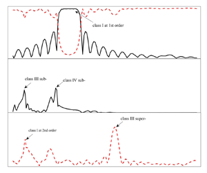
Figure 3. Parameters introduced for investigating nonlinear behaviours of class III Bragg resonances.
Hence,  $K^{(2)}_{Tm}$ represents either the maximum transmission or the maximum reflection coefficient of the second harmonic wave across the frequency range considered, and
  $A^{(2)}_{Tm}$ the corresponding maximum amplitude (i.e.
  $K^{(2)}_{Tm} = A^{(2)}_{Tm}/a^{(1)}$);
  $\omega ^{(2)}_p$ (the corresponding wavenumber denoted
  $k^{(2)}_p$) is the peak frequency at which
  $K^{(2)}_{Tm}$ actually occurs (i.e. the actual Bragg resonance points). It is noted that
  $\omega ^{(2)}_p$ or
  $k^{(2)}_p$ could be different from the linearized Bragg resonance points
  $\omega ^{(2)}_t$ or
  $k^{(2)}_t$ provided by Liu & Yue (Reference Liu and Yue1998); the difference of which is of concern and is investigated in this study.
Bailard, DeVries & Kirby (Reference Bailard, DeVries and Kirby1992) considered a Bragg breakwater as an effective shore-protection device if it can reflect more than 50 % of the incident wave energy. Thus,  $\omega ^{(2)}_{+}$ and
  $\omega ^{(2)}_{-}$ are defined as the frequencies at which
  $0.5K^{(2)}_{Tm}$ occurs, and the effective frequency bandwidth
  $\Delta {\omega ^{(2)}} = \omega ^{(2)}_{+} - \omega ^{(2)}_{-}$ in this work. Note that this is different from the conventional definition of the effective frequency bandwidth, e.g. in Wen & Tsai (Reference Wen and Tsai2008). The conventional bandwidth is the distance (across the frequency axis) between the adjacent frequencies at which zero coefficients occur.
The effects of surface and bottom waves on the characteristics of class III Bragg resonance in terms of the three parameters defined above are detailed in this section. To achieve this, six distinct sets of numerical experiments are designed; three (denoted Group 1–Group 3) for investigating the super-harmonic Bragg resonance, and three (denoted Group 4–Group 6) for the sub-harmonic Bragg resonance. The number of bottom ripples is varied from 2 to 13 in Group 1 and Group 4, the wave steepness varies in Group 2 and Group 5 and the amplitude of the ripples is varied in the range of 0.096–0.67 in Group 3 and Group 6. The testing conditions are also summarized in table 1.
Table 1. Testing conditions of class III Bragg super-/sub-harmonic resonance.

Note that the variation range of the wave steepness in Group 5 is smaller than that of Group 2. Class III Bragg sub-harmonic resonance is supposed to occur at rather small surface wave frequencies, which leads to a relatively large Ursell number on the weather side of the bottom structure. For this large wave steepness/Ursell number, stronger nonlinearity and possible wave breaking are thus expected, which could reach the limit of the current numerical method.
3.1. Amplitude of class III Bragg resonant waves
Liu & Yue (Reference Liu and Yue1998) indicated that the amplitude of a class III Bragg resonant wave is quadratic in the surface wave slope and linear in the bottom steepness, according to their regular perturbation solutions up to third order. The corresponding maximum values should increase linearly with the length of the periodic bottom structure.
Thus, the effects of surface and bottom waves on characteristics of class III Bragg resonant waves are firstly investigated by demonstrating the variations in amplitude of both the resonant transmitted and reflected waves with the parameter of  $n[k^{(1)}a^{(1)}]^{2}(k_bb)$, as shown in figure 4. It can be seen that the use of this parameter has led to a significant collapse of the data for all values of the wave steepness and the length of the bottom ripples. This collapse suggests that both the resonant transmitted and reflected waves indeed increase quadratically and linearly with the surface wave steepness and the structure length, respectively, as suggested by Liu & Yue (Reference Liu and Yue1998). However, it is found that the results of the resonant transmitted wave start to deviate significantly from this trend when the amplitude of the bottom ripples
  $b/h$ equals or is larger than 0.48 – see figure 4(a). The assumption of the small bottom wave slope inherent in the perturbation solution of Liu & Yue (Reference Liu and Yue1998) may no longer be valid for the cases with this large structure height. It is noted that the deviation in resonant reflected waves is less obvious (see figure 4b), which may be due to the fact that the variation range of
  $n[k^{(1)}a^{(1)}]^{2}(k_bb)$ is smaller when compared with that for the resonant transmitted waves. The selection of the variation range was discussed previously.

Figure 4. Variations in the amplitude of the super-harmonic resonant transmitted waves (a) and the sub-harmonic resonant reflected waves (b) with the wave and the bottom steepness, as well as the length of the periodic structure, represented by the parameter  $n[k^{(1)}a^{(1)}]^{2}(k_bb)$.
The amplitude of the resonant transmitted waves under class III Bragg resonance has then been plotted as a function of a new parameter  $n[k^{(1)}a^{(1)}]^{2}(k_bb)^{2}$ in figure 5. The collapse of the data is better, suggesting that the amplitude of the resonant waves, especially resonant transmitted waves, has a quadratic relationship with both the bottom and surface wave slopes, while still having a linear relationship with the structure length when the nonlinearity of the system increases. We note here that this quadratic dependence on the bottom steepness maybe altered by varying the bottom steepness to certain ranges, e.g. the linear dependence is found to work for smaller (non-dimensional) bottom structures, as discussed above and in Liu & Yue (Reference Liu and Yue1998).

Figure 5. Variations in the amplitude of the super-harmonic resonant transmitted waves with the new parameter  $n[k^{(1)}a^{(1)}]^{2}(k_bb)^{2}$.
3.2. Actual class III Bragg resonance conditions
The frequencies of the peak resonant transmitted or reflected waves  $\omega ^{(2)}_p$ (i.e. actual Bragg resonance conditions) relative to the linearized solutions
  $\omega ^{(2)}_t$ are investigated in figures 6–8. The resonant wave frequency/number shifting (either upshifting or downshifting) can in general be attributed to the nonlinear effects involved. Peng et al. (Reference Peng, Tao, Fan, Zheng and Liu2022) derived the theoretical solutions of frequency downshifting for class I Bragg resonance based on a regular perturbation analysis up to third order, and found that the frequency shifting has a quadratic dependence on the bottom/surface wave steepness. Hence, the variations in the actual class III Bragg resonance conditions are plotted against
  $(k^{(1)}a^{(1)})^{2}$ (representing the surface wave nonlinearity) and
  $(k_bb)^{2}$ (representing the bottom nonlinearity) in figures 7 and 8, respectively.

Figure 6. Shifting of the resonant frequency under class III Bragg resonances with the ripple number.

Figure 7. Shifting of the resonant frequency under class III Bragg resonances with the surface wave nonlinearity represented by  $(k^{(1)}a^{(1)})^{2}$.

Figure 8. Shifting of the resonant frequency under class III Bragg resonances with the bottom nonlinearity represented by  $(k_bb)^{2}$.
It can be seen that a general trend of upshifting (i.e. the actual Bragg resonance conditions are larger than the equivalent linearized solutions; the vertical axis is larger than 0) is found for the resonant transmitted waves, i.e. class III super-harmonic resonant waves (solid symbols in the figures). The level/extent of the upshift increases with the system nonlinearity represented by the parameters  $n$,
$n$,  $[k^{(1)}a^{(1)}]^{2}$ and
  $(k_bb)^{2}$. Note that a downshift is, however, found for the relatively smaller system nonlinearity, i.e. when
  $n < 4$,
  $[k^{(1)}a^{(1)}]^{2} < 0.0015$ and
  $(k_bb)^{2} < 0.2$.
According to Peng et al. (Reference Peng, Tao, Fan, Zheng and Liu2022), the nonlinear frequency correction introduced by the inclusion of third-order bottom and surface nonlinearities consists of three components. The first two, associated with the third-order interactions of bottom ripples with the second-order wave components that have wavenumbers of ( $k^{(1)}+k_b$) and (
 $k^{(1)}-k_b$), respectively, cause the surface wave frequency to shift downwards when compared with the linear solutions. The level/extent of the frequency downshift increases first with the surface wavenumber to its maximum value at (
 $2k^{(1)}/k_b$ = 1) and decreases with further increase in the wavenumber, and is found to have a quadratic relation with the bottom steepness,
  $k_bb$. This explains the increase observed in figure 7, despite the fact that the bottom steepness is kept unchanged in Group 2 and Group 5. We note here that the incident wave amplitude
  $a^{(1)}$ is constant and the wave steepness is changed by varying the incident wavenumber in this work. In contrast, the third term is associated with the third-order self-interaction of the propagating surface wave (analogous to a third-order Stokes wave), and leads to a frequency upshift that has a quadratic dependence on the surface wave steepness,
  $k^{(1)}a^{(1)}$.
These (nonlinearities from bottom waves; the first two terms mentioned above, and from surface waves; the aforementioned third term), in turn, result in an increase (upshift) and a decrease (downshift) of the resonant wavenumber of class III super-harmonic resonant waves, respectively. The final shifting is determined by the combined effects of these two; recall that  $k_b = k_p - 2k^{(1)}$ for the resonant transmitted waves.
An opposite trend is true for the resonant reflected waves, i.e. class III sub-harmonic resonant waves (open symbols in the figures), as now  $k_b = 2k^{(1)}+k_p$; recall that the wavenumber in this work is a scalar, and hence no information on its direction is provided.
This is different to class I Bragg resonance for which a downshift by bottom nonlinearity and an upshift by surface wave nonlinearity are found (Peng et al. Reference Peng, Tao, Fan, Zheng and Liu2022). Note that  $2k^{(1)}/k_b = 1$ for class I Bragg resonance, and
  $(2k^{(1)}\pm {k_b})/k^{(2)}_t = \pm 1$ for class III Bragg resonance; the plus signs are taken for the transmitted waves and the minus sign for the reflected waves.
The bottom nonlinearity plays a more important role when the parameters  $n$,
$n$,  $[k^{(1)}a^{(1)}]^{2}$ and
  $(k_bb)^{2}$ increase, as discussed previously. Thus, for larger system nonlinearity represented by these parameters, the peak class III Bragg resonant transmission and reflection are shifted to higher and lower wavenumbers relative to the linearized Bragg resonance points, respectively (see figures 6–8).
3.3. Effective frequency bandwidth of class III Bragg resonance
The effects of the surface and bottom waves on the effective frequency bandwidth  $\Delta \omega ^{(2)}$ are investigated in figures 9–11, respectively. It can be seen that the effective frequency bandwidth (for both the super- and sub-harmonic resonant waves) decreases with both the structure length
  $n$ (see figure 9) and the surface wave steepness
  $k^{(1)}a^{(1)}$ (see figure 10), although the decrease with the latter is mild. In contrast, an increase with the bottom slope
  $k_bb$ (i.e. the ripple amplitude; see figure 11) is observed. These trends are consistent to those for class I Bragg resonance, see e.g. Davies & Heathershaw (Reference Davies and Heathershaw1984). In addition, it is found that the bandwidth for the resonant transmitted waves is always smaller than that for the resonant reflected waves.

Figure 9. Variations in the effective frequency bandwidth with the ripple number.

Figure 10. Variations in the effective frequency bandwidth with the surface wave steepness.

Figure 11. Variations in the effective frequency bandwidth with the bottom slope.
4. Harmonic generation at Bragg resonances
It is well established that waves propagating over a submerged structure may introduce significant harmonic generation (i.e. redistribution of wave energy from the fundamental frequency into higher harmonics of this linear component) due to nonlinearity in both the incident waves and wave–structure interactions (e.g. shoaling effects). For example, Dick & Brebner (Reference Dick and Brebner1969) claimed that up to 64 % of the wave energy transmitted behind a submerged breakwater is transferred to higher harmonics of the incident wave. Harmonic waves up to at least fourth order are identified by Christou, Swan & Gudmestad (Reference Christou, Swan and Gudmestad2008) for waves interacting with rectangular submerged breakwaters.
These higher harmonic waves together with the linear wave components as well as the wavy bottom may satisfy the resonance conditions at various orders (Liu & Yue Reference Liu and Yue1998) to generate resonant waves that are of the same order of magnitude as the linear components. For example, class III Bragg resonance mentioned above (i.e. resonance at third order) is associated with the second harmonic waves. These resonant waves may in turn alter the underlying mechanisms associated with harmonic generation, and hence the local wave field. The former (i.e. the possible introduction of various Bragg resonances) will be discussed in the next section and this section is focused on the latter, i.e. harmonic generation at Bragg resonances, to investigate the interplay between these two phenomena.
We start with spatial distributions of the total free surface elevation along the centreline of the wave flume for cases with ( $\omega ^{(1)} = 6.11\,{\rm rad}\ {\rm s}^{-1}$) and without (
 $\omega ^{(1)} = 6.65\,{\rm rad}\ {\rm s}^{-1}$) the occurrence of class III super-harmonic Bragg resonance, as shown in figure 12. The results are collected at
  $t = 38T^{(1)}$ when the solutions are considered to have achieved steady states. A highly distorted free surface is observed above and behind the periodic structure when the Bragg resonance occurs, as expected. It is also not surprising to see that the corresponding linear solutions are reasonably smooth, indicating that the resonance mainly occurs in higher-order nonlinear components of wave–periodic structure interactions. As mentioned above, the resonant transmitted wave is exited at second order for the present bottom configuration;
  $\omega ^{(2)}_p = \sqrt {(gk_p\,{\rm tanh}{k_ph})} = 12.04\,{\rm rad}\ {\rm s}^{-1} \sim 2\omega ^{(1)} = 2 \times 6.11$.

Figure 12. Spatial distribution of the total and linear free surface elevations along the centreline of the wave flume for cases with (a) and without (b) the occurrence of class III super-harmonic Bragg resonance. The incident wave amplitude  $a^{(1)}=0.01$ m, the bottom slope
  $k_bb = 0.628$, the structure amplitude
  $b/h=0.48$ and the ripple number
  $n=5$. The black dash-dotted lines indicate the limits of the periodic bottom structure.
To demonstrate this effect more clearly, the spatial distribution of the higher-order nonlinear wave components at class III super-harmonic Bragg resonance (i.e. the difference between the total signal and the linear solutions shown in figure 12a) is shown in figure 13. The analytical solution of Liu & Yue (Reference Liu and Yue1998) is also given for direct comparison. It is clear that the Bragg resonant wave amplitude grows linearly with the propagation distance above the periodic structure, and fluctuates marginally around a nearly constant value behind the structure. When the resonance occurs, the wave amplitude of the higher harmonic wave is of the same order as the linear component; the crest value of the higher harmonic wave is up to  ${\sim }60\,\%$ of the linear solution. Both solutions from the present numerical model and Liu & Yue (Reference Liu and Yue1998) capture this trend well, although small differences between the two solutions are observed. In addition to the resonant transmitted wave at second order (free wave component), the nonlinear wave components calculated from the present numerical model also include second-order locked waves and wave components at frequencies that are higher than second order.

Figure 13. Spatial distribution of the higher-order nonlinear wave components. Black line: solutions from the present numerical model; red dashed line: analytical solution from Liu & Yue (Reference Liu and Yue1998). The black dash-dotted lines indicate the limits of the periodic bottom structure. For additional information refer to figure 12.
We summarize the spatial distribution of the second harmonic waves (both free and bounded wave components at double frequency are included) along the wave flume centreline at class III super- and sub-harmonic Bragg resonances in figure 14. It can be seen that standing waves are formed in front of the bottom structure, resulting from the superposition of linear incident and reflected waves. The phenomenon of beating (i.e. periodic oscillations in space) is observed to occur at the top of, or behind, the periodic bottom structure when the free and bounded second harmonic waves are in phase, and are of the same order. The beating value at the top of the structure increases and decreases with the travel distance over the structure for class III super- and sub-harmonic resonances, respectively. These trends agree well with those predicted by Liu & Yue (Reference Liu and Yue1998).

Figure 14. Spatial distribution of the linear wave component (black lines) and the second harmonics (red dashed lines) along the centreline at class III super-harmonic (a) and sub-harmonic (b) resonances. The black dash-dotted lines indicate the limits of periodic structure, and blue dashed lines are analytical solutions from Liu & Yue (Reference Liu and Yue1998). Here,  $(n)$ = (1) and (2).
Likewise, figure 15 shows the spatial distribution of the second harmonics along the wave flume centreline at class I Bragg resonance. Three bottom structure amplitudes ( $b/h = 0.16, 0.32$ and 0.48) are considered, and the result for the flat bed (
 $b/h= 0$) is also included for direct comparison. The phenomenon of beating is also observed to occur at the top of, or behind the periodic bottom structure. The beating length predicted by the current NWT is
  $\sim 1.975$ m, close to 1.939 m calculated by the theoretical formula
  $2{\rm \pi} /(k^{(2)}-2k^{(1)})$ in which
  $k^{(2)}$ is the wavenumber of the second-order free waves, and
  $k^{(1)}$ of the linear component (Hansen & Svendsen Reference Hansen and Svendsen1974).

Figure 15. Spatial distribution of the second harmonic waves along the centreline at class I Bragg resonance for various structure amplitudes. Here,  $b/h = 0$ indicates there is no periodic structure, and the black dash-dotted lines indicate the limits of the periodic structure.
Interestingly, additional beats are observed to occur and ride on top of the original beating before the bottom structures, leading to a maximum value of the second harmonic wave crest up to 5 times as large as that of the incident wave at second order (represented by the flat bottom case,  $b/h = 0$; top in the figure). This is denoted ‘parasitic beating’ and occurs when free and bounded second harmonic incident and reflected waves are in phase. It is noted that these four components are required to be of the same order for ‘beating’ and ‘parasitic beating’ to manifest, which is achieved by Bragg resonances. The maximum values of beating decrease with an increase of bottom structure amplitude when more energy is reflected. Hence, an opposite trend is found for the ‘parasitic beating’ in front of the structure. The detailed derivation and the mathematical elucidation of the phenomena of ’beating’ and ’parasitic beating’ can be found in Appendix B.
It is worth mentioning that the free second harmonic incident wave components shown in figure 15 top (i.e. the flat bed) are introduced due to the imperfect match between the wave generation at the inlet boundary and the applied/inherent fully nonlinear free surface boundary condition. The water particle motion cannot be produced exactly. This also occurs for physical experiments, as indicated by e.g. Hansen & Svendsen (Reference Hansen and Svendsen1974). Various methodologies have been developed in an attempt to minimize this mismatch, including the adoption of higher-order wave theories for specifying the fluid velocity at the inlet for numerical simulations (Anbarsooz, Passandideh-Fard & Moghiman Reference Anbarsooz, Passandideh-Fard and Moghiman2013), and the use of a non-sinusoidal time variation of the wave paddle motion in physical experiments (Hansen & Svendsen Reference Hansen and Svendsen1974). Despite these measures, it is well established that the perfect match is still hard (or impossible) to achieve.
Recall that the wave theory recommended by Le Méhauté (Reference Le Méhauté2013) for the wave parameters considered is the second-order Stokes wave theory, which is then applied in this work for wave generation (see (A7) in Appendix A). The generation of the ‘artificial’ free second harmonic ‘incident’ wave component is improved. For example, for the cases shown in figure 15, the ratio between the generated free second harmonic incident wave component and the linear wave component is  ${\sim }1.7\,\%$. This is smaller than
  ${\sim }5.8\,\%$ which is predicted by using the linear wave theory for wave generation.
Numerical simulations with various combinations of water depth and wave period (without the periodic structure in place) show that the ratio between this ’artificial’ free second harmonic incident wave component and the linear wave ranges from 1.2 % to 3 %; smaller for a larger water depth and a smaller wave steepness. For the case shown in figure 15, the bounded second harmonic incident wave component is approximately 4.3 % of the linear wave component (close to the theoretical prediction of  ${\sim }4.5\,\% = k^{(1)}a^{(1)}\,\mathrm {cosh}(k^{(1)}h)(2\,\mathrm {cosh}^{2}(k^{(1)}h)+1)/4\,\mathrm {sinh}^{3}(k^{(1)}h))$. The free and bounded second harmonic reflected wave components are up to
  $\sim 5\,\%$ of the linear wave component; larger for a higher bottom structure. Thus, all four components at second order are of the same order, and the aforementioned ‘parasitic beating’ is excited.
It is noted that the absolute values for these four wave components at second order are relatively small considering that the linear wave amplitude here is 0.01 m. This is reasonable and expected because class I Bragg resonance is exited in a linear fashion, as discussed before. Nevertheless, this scenario (i.e. free and bounded higher harmonic incident and reflected waves are of the same order) and the relevant conclusion are still useful as wave components of various wave frequencies co-exist in real seas.
We also note that, although the introduction of this small ’artificial’ free second harmonic incident wave in the system is unintentional, its existence did not affect the investigation of higher-order/nonlinear Bragg resonance (the focus of the present work). Hence, no further improvement in the wave generation is made.
The parasitic beating is not observed, however, for class III Bragg resonance, as shown in figure 14. This is due to the fact that only the incident bounded and the incident free second-order waves (rather than all four components mentioned above) are actually of significance for class III super-harmonic Bragg resonance, while the incident bounded and the reflected free second-order waves dominate class III sub-harmonic Bragg resonance.
5. Multi-Bragg resonance system
We now move on to investigate if the higher harmonic waves, hence the complex local wave field close to the periodic structure mentioned above, would introduce Bragg resonance at various orders. That is, if a multi-Bragg resonance system exists for the same bottom configuration.
Figure 16 summarizes the transmission and reflection coefficients of both the linear and second-order free wave components for various surface wave conditions studied in this work. Note that these are example results for the relatively large bottom configuration, i.e.  $b/h = 0.48$, for which we expect a stronger nonlinearity. It is clear that there are five relatively large peaks; 1 for the reflection curve of the linear component (a), 2 for the reflection curve of the second-order free waves (b) and 3 for the transmission curve of the second-order free waves (c).

Figure 16. Reflection and transmission coefficients for waves over a periodic structure with  $k_bb = 0.94$,
  $b/h = 0.48$ and
  $n = 10$, showing that multi-Bragg resonances occur for the same bottom configuration. The incident wave amplitude
  $a^{(1)} = 0.01$ m. Panels (a) to (c) show: reflection and transmission coefficients of the linear wave component, reflection coefficients of the second-order free waves, and transmission coefficients of the second-order free waves, respectively. The blue arrows indicate the linearized Bragg resonance points derived in Liu & Yue (Reference Liu and Yue1998).
The peak in the linear reflection coefficient curve should correspond to the classic class I Bragg resonance incurred by the linear wave component that has a wavenumber of  $k^{(1)}$. As expected,
  $2k^{(1)}/k_b \sim 1$ here, which is indicated by the bottom horizontal axis in figure 16(a). A small shift in the actual Bragg resonance points, and a larger effective frequency bandwidth, are also expected due to the strong nonlinearity involved, as discussed above in § 3.
For the reflection coefficient curve of the second-order free waves (b), the expected peak at  $(2k^{(1)}-k_b)/k^{(2)} \sim (-1)$ is observed close to which class III sub-harmonic Bragg resonance occurs. Recall that the wavenumber in this work is a scalar, and hence no information on the direction is provided. Thus, the minus sign in front of 1 indicates that this is for the reflected wave. In addition, another strong reflection at
  $(2k^{(1)}-k_b)/k^{(2)} \sim (-0.14)$ is observed. After a throughout analysis, it is found that the surface wavenumbers of the first and second harmonic waves,
  $k^{(1)}$ and
  $k^{(2)}$, and the bottom wavenumber
  $k_b$ here satisfy a relationship of
  $2k^{(1)}+k^{(2)}-2k_b = 0$, as indicated by the top horizontal axis. This follows the generalized Bragg conditions at
  $m = 4$ in Liu & Yue (Reference Liu and Yue1998)
 \begin{equation} \left. \begin{gathered} k_{(1)} \pm k_{(2)} \pm k_{(3)} \pm k_{b1} \pm k_{b2} = 0,\\ \omega_{(1)} \pm \omega_{(2)} - \omega_{(3)} =0 . \end{gathered} \right\} \end{equation}
 For the case of  $k_{(1)} = k_{(2)} = k^{(1)}$, and
  $k_{b1} = k_{b2} = k_b$
 \begin{equation} \left. \begin{gathered} k^{(2)} = k_{(3)} = 2k^{(1)} \pm 2k_b,\\ \omega^{(2)} = \omega_{(3)} = 2\omega^{(1)}. \end{gathered} \right\} \end{equation}
This Bragg resonance is then denoted class IV Bragg resonance, following the convention of Liu & Yue (Reference Liu and Yue1998). This type of Bragg resonance is captured, for (we believe) the first time, by either numerical or physical experiments.
Peaks in the transmission coefficient curve of the second-order free waves at  $(2k^{(1)}+k_b)/k^{(2)} \sim 1$ and
  $(2k^{(1)}+k_b)/k^{(2)} \sim 2.82$ (c) can also be found. The former corresponds to class III super-harmonic Bragg resonance at second order, consistent with that in Liu & Yue (Reference Liu and Yue1998). While the latter is found to overlap with class III sub-harmonic Bragg resonance condition at which the second-order reflected wave is significant due to the resonance (cf.
  $(2k^{(1)}-k_b)/k^{(2)} \sim (-1)$; b). Note that for the condition of
  $(2k^{(1)}+k_b)/k^{(2)} \sim 2.82$,
  $k^{(2)}$ equals 3.29 m
 $^{-1}$ and we know that the bottom wavelength
  $k_b = 2{\rm \pi}$ m
 $^{-1}$. That is,
  $2k^{(2)}/k_b \sim 1$, suggesting that class I Bragg resonance condition is satisfied here. Class I Bragg resonance at second order is excited here by the resonant reflected waves of class III Bragg resonance.
We note that the formation mechanism for the smallest peak (among the five) is still under exploration, and we leave this for the future.
We highlight that this multi-Bragg resonance system is of importance as, in practical applications, the incident wave field often contains multiple wave components. They themselves and their combinations may satisfy the resonance conditions to generate resonant waves. These resonant waves may then satisfy and/or engage in multiple resonances with the incident components, e.g. the observed class I Bragg resonance at second order in figure 16. The wave field becomes increasingly complex, and may generate a certain type of wave, e.g. long infragravity, that is of special importance to coastal processes and engineering applications.
The spatial distributions of the free surface elevation along the centreline of the wave flume at  $t = 45T^{(1)}$ under the aforementioned class IV Bragg resonance condition are shown in figure 17. Similar to figure 12, both linear and nonlinear solutions are included. As expected, a highly distorted wave profile (even more distorted than that in figure 12 for class Bragg III resonance) is found in nonlinear solutions before and above the periodic structures, suggesting that resonance is actually excited in nonlinear higher harmonic reflected waves. This is consistent with the mathematical behaviour in (5.1)–(5.2).

Figure 17. Spatial distribution of the free surface elevation along the centreline of the wave flume at  $t = 45T$ at class IV Bragg resonance. The black dash-dotted lines indicate the limits of the periodic bottom structure.
6. Conclusions
In this work, numerical simulations are carried out to investigate nonlinear waves propagating over a periodic structure, and the subsequent Bragg resonant waves. The numerical model, the so-called fully nonlinear NWT, solves the Poisson equation as well as the fully nonlinear kinematic and dynamic free surface boundary conditions based on the HOBEM in time domain. This allows the various nonlinearity involved to be considered properly.
The numerical results are verified by comparing with the published experimental measurements on class III Bragg resonance, and are extended to explore the hydrodynamic behaviours of the system to a wider range of surface and bottom waves of practical interest. Thus, the fully nonlinear NWT is demonstrated to be an effective tool for exploring the physics of wave–multi-structure interactions that leads to various types of Bragg resonance. Accurate predictions of the local wave field and transmitted as well as reflected waves are obtained.
Six distinct sets of numerical experiments are carefully designed to explore the characteristics of class III Bragg resonance extensively. The results show that the amplitudes of both Bragg resonant reflected and transmitted waves increase quadratically and linearly with the surface wave steepness, and the ripple number of the periodic structure, respectively. This is consistent with the perturbation solutions by Liu & Yue (Reference Liu and Yue1998). However, there is a quadratic rather than linear relationship (e.g. as suggested by Liu & Yue Reference Liu and Yue1998) with the bottom slope if the bottom size increases to a certain level, i.e.  $b/h$ equals or is larger than 0.48 in this work. In this case, the assumption of small ripple amplitude in the perturbation solutions may no longer be valid. Accordingly, a new parameter of
  $n[k^{(1)}a^{(1)}]^{2}(k_bb)^{2}$ is introduced to characterize class III Bragg resonance, which further emphasizes the bottom nonlinearity.
It is found that the extent of the frequency shift (the difference between the actual Bragg resonance conditions and the corresponding linearized solutions) becomes more significant when the system nonlinearity (represented by the parameters  $n$,
$n$,  $[k^{(1)}a^{(1)}]^{2}$ and
  $(k_bb)^{2}$) increases. Generally, the nonlinearities in surface and bottom waves would decrease and increase the free surface wavenumber, respectively. The latter is found to be dominant when the bottom size increases to a certain level, as discussed above. Thus, at larger
  $n$,
$n$,  $[k^{(1)}a^{(1)}]^{2}$ and
  $(k_bb)^{2}$), an upshift is found for class III super-harmonic Bragg resonance, while a downshift for class III sub-harmonic Bragg resonance is observed. This contrasts with the widely studied class I Bragg resonance for which a downshift is always observed. It is the coupling of these two opposite effects rather than the nonlinearity arising from each alone that is of importance. Additionally, the effective frequency bandwidth is found to increase with the bottom slope, while it decreases with the wave steepness and the ripple number.
Higher harmonic generation over a submerged periodic structure at Bragg resonances is also investigated. The interplay between these two phenomena (i.e. harmonic generation and Bragg resonance) are of concern. The phenomena of beating (i.e. periodic oscillations in space) and parasitic beating (i.e. additional beating riding on top of the original one) are observed at the top of, and/or behind the periodic bottom structure. These occur when the free and bounded second harmonic (transmitted and/or reflected) waves are of the same order (induced by the Bragg resonances) and are in phase, leading to a large local water surface motion (up to 5 times of the corresponding bounded waves) in front of the depth transition. This could play an important role in an enhanced probability of extreme waves on wavy bottom.
Various types of Bragg resonance, i.e. a multi-Bragg resonance system, are observed, including the well-known class I and III Bragg resonances that occur in linear components at close to the incident wave frequency, and second harmonic components at frequencies that are close to twice the fundamental frequency, respectively. In addition, class I Bragg resonant transmitted waves at second order and class IV Bragg resonant reflected waves at second order are captured, for (we believe) the first time, by numerical experiments. Class IV Bragg resonance is a result of free surface and bottom nonlinearities involving resonant interaction among two bottom and three surface wave components. This multi-resonance system is of significance for investigating the behaviours of the local wave field near the shore, and designing the so-called Bragg breakwaters.
Funding
This work is supported by LiaoNing Revitalization Talents Program (Grant No. XLYC2002033); Liaoning BaiQianWan Talents Program (Grant No. 2020921007) and Fundamental Research Funds for the Central Universities (Grant No. DUT21LAB116). We are also grateful for the support of the National Natural Science Foundation of China (grant no. 52001053).
Declaration of interests
The authors report no conflict of interest.
Appendix A. Numerical methods
This appendix presents the details (theoretical formulation, solution algorithm etc.) of the numerical method, i.e. the fully nonlinear NWT, employed in this work.
A.1. Theoretical formulation
The Cartesian coordinate system shown in figure 1 is used, i.e. the horizontal  $x$-axis and the vertical
  $z$-axis are positive when pointing to the right and upwards, respectively, and
  $x = 0$ is defined at the left end of the domain (excluding the damping zone in the left) and
  $z = 0$ is on the mean water level.
Let  $t$ denote the time, the velocity potential
  $\phi (x,z,t)$ is then introduced to describe the fluid motion in the NWT, assuming that the fluid is incompressible, inviscid and the flow is irrotational and two-dimensional. The Laplace equation (i.e.
  $\nabla ^{2}\phi (x,z,t)=0$) is generally used to accurately describe the behaviour of velocity potentials in the whole computational domain. However, because we use the method of source generation for generating incident waves in this work (details to follow), the Poisson equation is used instead (Brorsen & Larsen Reference Brorsen and Larsen1987)
 \begin{equation} \nabla^{2}\phi(x,z,t)=q^{{\ast}} \end{equation}
where  $q^{\ast }=q^{\ast }(x_s,z)$ is the volume flux density of the source distribution, and is related to the incident wave kinematics (details to follow). Here,
  $x_s$ is the horizontal position of the vertical source distribution, which is 0 in this work (i.e. at the left end of the computational domain excluding the damping zone in the left).
As shown in figure 1, the fluid is bounded by the left inlet boundary  $S_{I}$, the bottom
  $S_B$ (including both the horizontal seabed
  $S_{hb}$ and the periodic structure
  $S_b$), the outflow boundary
  $S_O$ and the free surface
  $S_F$. Each boundary should satisfy the corresponding boundary condition to complete the BVP considered.
On the free surface  $S_F$ we have both fully nonlinear kinematic and dynamic boundary conditions
 \begin{equation} \left. \begin{gathered} {\frac{\partial\eta}{\partial{t}} = \frac{\partial\phi}{\partial{z}} - {\frac{\partial\phi}{\partial{x}}}{\frac{\partial\eta}{\partial{x}}}},\\ \frac{\partial\phi}{\partial{t}} ={-} g\eta-\frac{1}{2}|\boldsymbol{\nabla}\phi|^{2}, \end{gathered} \right\} \end{equation}
where  $\eta$ is the free surface elevation, and
  $g$ the acceleration due to gravity.
In this work, the hybrid Euler–Lagrangian method is used to track the instantaneous free surface, and the method of numerical beach is applied for absorbing reflected waves from the domain, should they be present. Hence, the free surface boundary conditions are re-written as
 \begin{equation} \left. \begin{gathered} {\frac{{\rm d}\boldsymbol{X}}{{\rm d}t} = \frac{\partial\phi}{\partial{z}} - \mu(x)(\boldsymbol{X}-\boldsymbol{X}_0)}, \\ \frac{{\rm d}\phi}{{\rm d}{t}} ={-} g\eta+\frac{1}{2}|\boldsymbol{\nabla}\phi|^{2}-\mu(x)\phi, \end{gathered} \right\} \end{equation}
where  $\textrm {d}/\textrm {d}t = \partial /\partial {t} + u\boldsymbol {{\cdot }}\boldsymbol {\nabla }$ in which
  $u$ is the fluid velocity,
  $\boldsymbol {X}=(x,z)$ is the instantaneous position of the water particle on the free surface and
  $\boldsymbol {X}_0=(x,0)$ is the position of the free surface at the initial stage, i.e. mean water level. The damping term
  $\mu (x)$ satisfies
 \begin{equation} \mu(x) = \left\{
\begin{array}{@{}ll}
\nu\left(\dfrac{x-x_{1,2}}{L_b}\right)^{2}, & x\leq x_1
\text{ or } x \geq x_2,\\ 0, & x_1 < x < x_2, \\
\end{array} \right. \end{equation}
\begin{equation} \mu(x) = \left\{
\begin{array}{@{}ll}
\nu\left(\dfrac{x-x_{1,2}}{L_b}\right)^{2}, & x\leq x_1
\text{ or } x \geq x_2,\\ 0, & x_1 < x < x_2, \\
\end{array} \right. \end{equation}
where  $\nu$ (= 1 in this work) is the damping coefficient, and
  $L_b$ is the length of the damping zones, which is selected as twice the wavelength
  $\lambda$ in this work;
  $x_1$ and
  $x_2$ are the starting positions of the left and right damping zones, respectively. Note that the values of
  $\nu$ and
  $L_b$ are empirically determined.
On the bottom  $S_B$ and at the outflow boundary
  $S_O$, the impermeable boundary condition is satisfied
 \begin{equation} \frac{\partial\phi}{\partial{n}} = 0, \end{equation}
where  $n$ is the unit normal vector.
As mentioned previously, the method of source generation is applied in which a set of pulsating sources are distributed evenly along the inlet boundary  $S_I$, extending from the bottom to the free surface. The desired waves are then generated by controlling the volume flux density of the vertical source distribution (Brorsen & Larsen Reference Brorsen and Larsen1987)
 \begin{equation} q^{{\ast}} = 2v\delta(x-x_s), \end{equation}
where  $\delta (x-x_s)$ is the Dirac delta function, and
  $v = v(x,z,t)$ is the horizontal fluid velocity corresponding to the wave we want to generate. The volume flux from the area
  $\textrm {d}y\,\textrm {d}z$ on the source distribution is
  $q^{\ast }\,{\textrm {d}y\,\textrm {d}z}$. Here,
  ${\textrm {d}y} = 1$ for two-dimensional flows. Note that a factor of 2 is introduced because two waves that propagate in opposite directions are generated simultaneously by the pulsating flux density.
In this work, the fluid velocity  $v$ at the inlet boundary
  $S_I$ is specified based on the second-order Stokes theory (Koo & Kim Reference Koo and Kim2007)
 \begin{align} v & = \frac{kga}{\omega}\frac{\text{cosh}k(z+h)}{\text{cosh}kh}\cos (kx-\omega{t}) \nonumber\\ & \quad+ \frac{3}{4}kga^{2}\omega\frac{\text{cosh}2k(z+h)}{\text{sinh}^{4}kh}\cos 2(kx-\omega{t}), \end{align}
where  $h$ is the water depth above the horizontal seabed,
  $a$ the incident wave amplitude,
  $\omega$ the incident wave circular frequency and
  $k$ the wavenumber satisfying the dispersion equation
 \begin{equation} \omega^{2} = gk\text{tanh}kh. \end{equation}
 It is noted that, without introducing any misunderstanding, the superscript  ${(1)}$ indicating the order of the wave components is omitted in this appendix for brevity.
The initial conditions are required in order to perform a time-domain analysis. Here, we assume that the free surface is stationary and flat initially
 \begin{equation} \left. \begin{aligned} \phi(x,z,0) & = 0, \\ \eta(x,0) & = 0. \end{aligned} \right\} \end{equation}
A.2. Boundary integral equation
The aforementioned BVP ((A1)–(A5)) can be reformulated as an integral equation by using the second Green's theorem (Brebbia & Walker Reference Brebbia and Walker2016)
 \begin{align} \alpha(p)\phi(p) & = \int_S \left[\phi(q)\frac{\partial{G(p,q)}}{\partial{n}}-G(p,q)\frac{\partial\phi(q)}{\partial{n}}\right] \,{\rm d}S \nonumber\\ &\quad + \int_{\varOmega} [q^{{\ast}}{G(p,q)}] \,{\rm d}\varOmega, \end{align}
where  $p = (x_0,z_0)$ is the source point,
  $q = q(x,z)$ is the field point and
  $\alpha (p)$ is the solid angle coefficient associated with the surface geometry of the source point position;
  $\varOmega$ is the volume of the computational domain, and the bounded surface of the computational domain
  $S$ consists of the free surface
  $S_F$, the periodic structure
  $S_b$, the inlet boundary
  $S_I$ and the outflow boundary
  $S_O$.
Here, the Green function  $G(p,q)$ is calculated to extend the computational domain by adding its mirror image with respect to the horizontal part of the seabed (Newman Reference Newman1992)
 \begin{equation} G(p,q) = \frac{1}{2{\rm \pi}}(\ln r_1 + \ln r_2), \end{equation}
where
 \begin{equation} \left. \begin{aligned} r_1 & = \sqrt{(x-x_0)^{2} + (z-z_0)^{2}},\\ r_2 & = \sqrt{(x-x_0)^{2}+(z+z_0+2~h)^{2}}. \end{aligned} \right\} \end{equation}
Hence,  $r_1$ is actually the distance between the field point and the source point, and
  $r_2$ is the distance between the field point and the image of the source point reflected about the bottom. In this case, the horizontal part of the seabed is excluded from the integral, reducing the computational effort.
The solid angle coefficient  $\alpha (p)$ is given by
 \begin{equation} \alpha(p) = \left\{ \begin{array}{@{}ll} 1, & \text{when } p \text{ is inside the domain},\\ 0, & \text{when } p \text{ is outside the domain},\\ 1-{\beta}/{2{\rm \pi}}, & \text{when } p \text{ is on the boundary surfaces},\\ \end{array} \right. \end{equation}
where  $\beta$ is the solid angle.
A.3. Higher-order boundary element method
The HOBEM is applied in this work to solve the boundary integral equation (A10) in which the boundary surface is discretized into a set of three-node elements for the 2-D wave tank. Note that for 3-D problems, the node number can also be eight or six for curved quadrilateral and triangular elements, respectively.
By introducing the quadratic shape function  $h_k(\xi )$ in each surface element, the position coordinate, the velocity potential and its derivatives within an element can be transformed to the local intrinsic coordinate system
  $(\xi,\eta )$, and can be represented in terms of nodal values in the following forms:
 \begin{equation} \left. \begin{aligned} \boldsymbol{X}(\xi,\eta) & = \sum_{k=1}^{K} h_k(\xi)\boldsymbol{X}_k,\\ \phi(\xi,\eta) & = \sum_{k=1}^{K} h_k(\xi)\phi_k ,\\ \frac{\partial\phi(\xi,\eta)}{\partial\xi} & = \sum_{k=1}^{K} \frac{\partial{h_k(\xi)}}{\partial\xi}\phi_k ,\\ \frac{\partial\phi(\xi,\eta)}{\partial\eta} & = \sum_{k=1}^{K} \frac{\partial{h_k(\xi)}}{\partial\eta}\phi_k, \end{aligned} \right\} \end{equation}
where  $K (=3)$ is the number of nodes in each element;
  $\boldsymbol {X}_k$ and
  $\phi _k$ are the nodal positions and potentials, respectively. The quadratic shape function
  $h_k(\xi,\eta )$ in this work is given by
 \begin{equation} \left. \begin{aligned} {h_1}(\xi) & = \frac{\xi(\xi-1)}{2},\\ {h_2}(\xi) & = (1+\xi)(1-\xi),\\ {h_3}(\xi) & = \frac{\xi(\xi+1)}{2}. \end{aligned} \right\} \end{equation}
 The elements are so-called isoperimetric elements as both the geometry/coordinates of each element and its dependent physical variables (e.g.  $\phi$ and its derivatives) are represented by the same shape function, as shown in (A14).
Substituting the representation of (A14) into (A10), the integral equation in discrete form can be formulated
 \begin{align}
&\alpha(\boldsymbol{X}_i)\phi(\boldsymbol{X}_i)-\sum_{j=1}^{N_{e_2}}
\int_{{-}1}^{1} \sum_{k=1}^{K}h_k(\xi)\phi_{jk}
\frac{\partial{G(\boldsymbol{X}_i,\boldsymbol{X}_j(\xi,\eta))}}{\partial{n}}|J_j(\xi)|\,{\rm
d}{\xi}\,{\rm d}{\eta} \nonumber\\ & \qquad +
\sum_{j=1}^{N_{e_1}} \int_{{-}1}^{1}
\sum_{k=1}^{K}h_k(\xi)G(\boldsymbol{X}_i,\boldsymbol{X}_j(\xi,\eta))
\frac{\partial{\phi_{jk}}}{\partial{n}}|J_j(\xi)|\,{\rm
d}{\xi}\,{\rm d}{\eta} \nonumber\\ & \quad =
\sum_{j=1}^{N_{e_1}} \int_{{-}1}^{1}\phi_j
\frac{\partial{G(\boldsymbol{X}_i,\boldsymbol{X}_j(\xi,\eta))}}{\partial{n}}|J_j(\xi)|\,{\rm
d}{\xi}\,{\rm d}{\eta} \nonumber\\ & \qquad -
\sum_{j=1}^{N_{e_2}}
\int_{{-}1}^{1}G(\boldsymbol{X}_i,\boldsymbol{X}_j(\xi,\eta))
\frac{\partial{\phi_{jk}}}{\partial{n}}|J_j(\xi)|\,{\rm
d}{\xi}\,{\rm d}{\eta} \nonumber\\ & \qquad +
\sum_{j=1}^{N_{e_3}}
\int_{{-}1}^{1}q^{{\ast}}{G(\boldsymbol{X}_i,\boldsymbol{X}_j(\xi,\eta))}|J_j(\xi)|\,{\rm
d}{\xi}\,{\rm d}{\eta}, \end{align}
\begin{align}
&\alpha(\boldsymbol{X}_i)\phi(\boldsymbol{X}_i)-\sum_{j=1}^{N_{e_2}}
\int_{{-}1}^{1} \sum_{k=1}^{K}h_k(\xi)\phi_{jk}
\frac{\partial{G(\boldsymbol{X}_i,\boldsymbol{X}_j(\xi,\eta))}}{\partial{n}}|J_j(\xi)|\,{\rm
d}{\xi}\,{\rm d}{\eta} \nonumber\\ & \qquad +
\sum_{j=1}^{N_{e_1}} \int_{{-}1}^{1}
\sum_{k=1}^{K}h_k(\xi)G(\boldsymbol{X}_i,\boldsymbol{X}_j(\xi,\eta))
\frac{\partial{\phi_{jk}}}{\partial{n}}|J_j(\xi)|\,{\rm
d}{\xi}\,{\rm d}{\eta} \nonumber\\ & \quad =
\sum_{j=1}^{N_{e_1}} \int_{{-}1}^{1}\phi_j
\frac{\partial{G(\boldsymbol{X}_i,\boldsymbol{X}_j(\xi,\eta))}}{\partial{n}}|J_j(\xi)|\,{\rm
d}{\xi}\,{\rm d}{\eta} \nonumber\\ & \qquad -
\sum_{j=1}^{N_{e_2}}
\int_{{-}1}^{1}G(\boldsymbol{X}_i,\boldsymbol{X}_j(\xi,\eta))
\frac{\partial{\phi_{jk}}}{\partial{n}}|J_j(\xi)|\,{\rm
d}{\xi}\,{\rm d}{\eta} \nonumber\\ & \qquad +
\sum_{j=1}^{N_{e_3}}
\int_{{-}1}^{1}q^{{\ast}}{G(\boldsymbol{X}_i,\boldsymbol{X}_j(\xi,\eta))}|J_j(\xi)|\,{\rm
d}{\xi}\,{\rm d}{\eta}, \end{align}
where  $N_{e_1}$,
  $N_{e_2}$ and
  $N_{e_3}$ are the number of elements on the free surface
  $S_F$, the periodic structure
  $S_b$ and at the inlet boundary
  $S_I$, respectively. At this stage,
  $\boldsymbol {X}_i$ is an arbitrary point on the free surface and other discretized boundaries, and
  $J_j(\xi )$ is the Jacobian relating the global coordinates and the local intrinsic coordinates in the
  $j$th element.
After assembling the equations for each element, we obtain the following set of linear equations:
 \begin{equation} [A]_{N_e\times {N_e}} = \left\{ \begin{array}{@{}c@{}} \dfrac{\partial\phi}{\partial{n}}\\ \phi \end{array} \right \}_{N_e} \\ = [B]_{N_e}, \end{equation}
where  $N_e = N_{e_1}+N_{e_2}$.
At a given time step, either the velocity potential or its normal derivative on each part of the boundary is known from the corresponding boundary conditions, and the rest can be obtained by solving the above discretized equations.
The boundary surfaces  $S$ are re-meshed and updated at each time step to maintain the quality of the mesh, i.e. to minimize the distortion of the mesh. Then the boundary integral equation is re-built and solved accordingly. The standard fourth-order Runge–Kutta method is used to advance the solution process in time, in an iterative manner. Once the (A17) is solved, the time histories of the free surface elevation at an arbitrary point inside the computational domain can be obtained for postprocessing, such as spectrum analysis and calculation of reflection/transmitted coefficients.
Appendix B. Mathematical elucidation of ‘beating’ and ‘parasitic beating’
If we include all terms to second order, the free surface elevation to second order  $\eta ^{(2)}$ at the weather side of the periodic structure can be written as the superposition of the bounded and free second harmonic incident and reflected wave components (neglecting the phase angle)
 $$\begin{align} \eta^{(2)} &=
a_{LI}^{(2)}\cos 2(k^{(1)}x-\omega^{(1)}t) +
a_{FI}^{(2)}\cos (k^{(2)}x-2\omega^{(1)}t) \nonumber\\ &\quad +
a_{LR}^{(2)}\cos 2(k^{(1)}x+\omega^{(1)}t)
+a_{FR}^{(2)}\cos (k^{(2)}x+2\omega^{(1)}t),
\end{align}$$
$$\begin{align} \eta^{(2)} &=
a_{LI}^{(2)}\cos 2(k^{(1)}x-\omega^{(1)}t) +
a_{FI}^{(2)}\cos (k^{(2)}x-2\omega^{(1)}t) \nonumber\\ &\quad +
a_{LR}^{(2)}\cos 2(k^{(1)}x+\omega^{(1)}t)
+a_{FR}^{(2)}\cos (k^{(2)}x+2\omega^{(1)}t),
\end{align}$$
where  $a_{LI}^{(2)}$,
  $a_{FI}^{(2)}$,
  $a_{LR}^{(2)}$ and
  $a_{FR}^{(2)}$ are the wave amplitudes of the bounded and free second harmonic incident and reflected wave components, respectively. The subscripts ‘L’ and ‘F’ denote that these are terms corresponding to locked/bounded and free waves, respectively and the subscripts ‘I’ and ‘R’ represent incident and reflected waves, respectively. As discussed previously, the free second harmonic incident wave is introduced to the system due to the mismatch between the wave generation at the inlet boundary and the applied fully nonlinear free surface boundary condition.
Equation (B1) can also be rewritten as (via trigonometric transformation)
 \begin{align} \eta^{(2)} & = \left(a_{LI}^{(2)}-a_{FI}^{(2)}-(a_{LR}^{(2)}-a_{FR}^{(2)})\right) \cos 2\left(k^{(1)}x-\omega^{(1)}t\right) \nonumber\\ &\quad + 2\left(a_{FI}^{(2)}-a_{FR}^{(2)}\right)\cos \left(\frac{2k^{(1)}-k^{(2)}}{2}x\right) \cos \left(\frac{2k^{(1)}+k^{(2)}}{2}x-2\omega^{(1)}t\right)\nonumber\\ &\quad + 2(a_{LR}^{(2)}\cos 2k^{(1)}x+a_{FR}^{(2)}\cos k^{(2)}x)\cos 2\omega^{(1)}t, \end{align}
where the second term represents the group effect, and the last two terms associated with the reflected waves are standing waves. Example spatial distributions of these four terms along the centreline of the wave flume are shown in figure 18 to show the variation of the wave motion envelopes. It is clear that the beating lengths (periodic variations of the envelopes) of these four terms are rather different, and their superposition results in the ‘parasitic beating’ if they are of the same order in magnitude. The beating length of the first term (figure 18a) can be considered to be infinite, i.e. there is no variation in the wave amplitude in space.

Figure 18. Example spatial distributions of wave components represented by the four terms in (B2) along the centreline of the wave flume at various time instants, showing the variation of the wave motion envelopes. From (a) to (d) are the results corresponding to the first, second, third and fourth terms, respectively.
If only two wave components (e.g. bounded and free second harmonic incident wave components) are of significance, the terms associated with reflected waves can then be dropped
 \begin{align} \eta^{(2)} & = (a_{LI}^{(2)}-a_{FI}^{(2)})\cos 2(k^{(1)}x-\omega^{(1)}t) \nonumber\\ &\quad + 2a_{LI}^{(2)}\cos \left(\frac{2k^{(1)}-k^{(2)}}{2}x\right)\cos \left(\frac{2k^{(1)}+k^{(2)}}{2}x-2\omega^{(1)}t\right). \end{align}
Again, the second term represents the group effect, and the distance between the two adjacent maximum or minimum values of this term is the beating length mentioned above. The beating length  $L$ satisfies
 \begin{equation} \tfrac{1}{2}(k^{(2)}-2k^{(1)})L={\rm \pi}. \end{equation}
Hence,
 \begin{equation} L=\frac{2{\rm \pi}}{k^{(2)}-2k^{(1)}}. \end{equation}


