


1 Introduction
The Vlasov–Maxwell description was adopted around the middle of the past century to formulate the linear theory of waves in finite-temperature, collisionless plasmas. Beginning with the simplest, electron-Langmuir wave, two different albeit equivalent approaches were developed. The first one was Landau’s (Reference Landau1946) method of analytic continuation and complex contour integration for the Laplace-transformed solution of initial-value problems. The second was Van Kampen’s (Reference Van Kampen1955) and Case’s (Reference Case1959) derivation of a complete basis of normal modes with harmonic time dependence, including the singular ones associated with a continuous frequency spectrum. These methods were subsequently used to study other plasma waves. However, following the comprehensive analysis of Bernstein (Reference Bernstein1958) based on Landau’s approach, this method became overwhelmingly the preferred one both in the research literature and in the classroom. Thus, standard plasma textbooks, whether general such as Krall & Trivelpiece (Reference Krall and Trivelpiece1973), Lifshitz & Pitaevskii (Reference Lifshitz and Pitaevskii1981), Goldston & Rutherford (Reference Goldston and Rutherford2000) and Hazeltine & Waelbroeck (Reference Hazeltine and Waelbroeck2004), or specialized in wave theory such as Stix (Reference Stix1962), Brambilla (Reference Brambilla1998), Pecseli (Reference Pecseli2012) and Bers (Reference Bers2016), present the theory of plasma waves according to Landau’s approach and perhaps apply Van Kampen’s normal-mode approach only to the discussion of the electron-Langmuir wave. Nevertheless, the normal-mode method has some specific virtues compared to the Laplace transform method. In particular, it makes clear the nature of the Landau damping as the result of the mixing of the phases of different spectral components of the perturbation, not normal modes with complex frequency. More importantly, it allows for initial conditions that do not necessarily have the analyticity properties required by the standard derivation of ‘effective dispersion relations’ (by way of analytic continuation and complex contour integration) in the Laplace transform approach.
The reason why a normal-mode-based theory of plasma waves as broad in scope as Bernstein’s (Reference Bernstein1958) Laplace-transform-based theory has not been available, can be attributed to the mathematical complexities of the former, as remarked in Bernstein’s paper itself. Such complexities have two distinct roots. The first one is the fact that, except for the special
 $k_{\Vert }=0$
case of wave propagation perpendicular to the equilibrium magnetic field, the spectrum of eigenfrequencies includes a continuum and this continuum is in general highly degenerate. The degeneracy of the continuum of eigenfrequencies arises from several causes. One is the multiple degrees of freedom corresponding to the number of plasma species and the three possible polarizations of the perturbed electromagnetic fields. Another and more insidious is the fact that many differently perturbed distribution functions of the three-dimensional velocity produce equivalent effects as far as the overall dynamics of the perturbation is concerned. Finally, one has to take into account the continuum of so-called ballistic modes, namely modes that perturb the distribution functions but do not perturb the electromagnetic fields. The continuum degeneracy difficulty is greatly alleviated if the equilibrium background has no magnetic field or if the wave propagation direction is parallel to the magnetic field of a magnetized equilibrium because, in these cases, a reduced problem can be formulated in terms of integrated distribution functions that depend only on the velocity component parallel to the propagation wavevector, after straightforward integration with respect to the perpendicular components. Moreover, for unmagnetized equilibrium or parallel propagation, the three electromagnetic polarization states are decoupled and can be analysed independently. Thus, most of the normal-mode-based research carried out so far has been limited to these unmagnetized equilibrium or parallel propagation situations (Van Kampen Reference Van Kampen1955; Pradhan Reference Pradhan1957; Case Reference Case1959; Felderhof Reference Felderhof1963a
,Reference Felderhof
b
; Van Kampen & Felderhof Reference Van Kampen and Felderhof1967; Lambert, Best & Sluijter Reference Lambert, Best and Sluijter1982; Ignatov Reference Ignatov2017). The works of McCune (Reference McCune1966) and Watanabe (Reference Watanabe1968) did tackle the far more difficult problem of wave propagation oblique to a non-zero equilibrium magnetic field. However, these works simplified the continuum degeneracy difficulty by considering a plasma with immobile ions and with the electrons as the single dynamical species, and by assuming an electrostatic approximation with only one polarization state. They derived perturbation solutions that resolved the dependence of the electron distribution function on the three-dimensional velocity, but no attempts were made to apply them to specific problems or to make contact with the results available from the Laplace-transform-based methodology.
$k_{\Vert }=0$
case of wave propagation perpendicular to the equilibrium magnetic field, the spectrum of eigenfrequencies includes a continuum and this continuum is in general highly degenerate. The degeneracy of the continuum of eigenfrequencies arises from several causes. One is the multiple degrees of freedom corresponding to the number of plasma species and the three possible polarizations of the perturbed electromagnetic fields. Another and more insidious is the fact that many differently perturbed distribution functions of the three-dimensional velocity produce equivalent effects as far as the overall dynamics of the perturbation is concerned. Finally, one has to take into account the continuum of so-called ballistic modes, namely modes that perturb the distribution functions but do not perturb the electromagnetic fields. The continuum degeneracy difficulty is greatly alleviated if the equilibrium background has no magnetic field or if the wave propagation direction is parallel to the magnetic field of a magnetized equilibrium because, in these cases, a reduced problem can be formulated in terms of integrated distribution functions that depend only on the velocity component parallel to the propagation wavevector, after straightforward integration with respect to the perpendicular components. Moreover, for unmagnetized equilibrium or parallel propagation, the three electromagnetic polarization states are decoupled and can be analysed independently. Thus, most of the normal-mode-based research carried out so far has been limited to these unmagnetized equilibrium or parallel propagation situations (Van Kampen Reference Van Kampen1955; Pradhan Reference Pradhan1957; Case Reference Case1959; Felderhof Reference Felderhof1963a
,Reference Felderhof
b
; Van Kampen & Felderhof Reference Van Kampen and Felderhof1967; Lambert, Best & Sluijter Reference Lambert, Best and Sluijter1982; Ignatov Reference Ignatov2017). The works of McCune (Reference McCune1966) and Watanabe (Reference Watanabe1968) did tackle the far more difficult problem of wave propagation oblique to a non-zero equilibrium magnetic field. However, these works simplified the continuum degeneracy difficulty by considering a plasma with immobile ions and with the electrons as the single dynamical species, and by assuming an electrostatic approximation with only one polarization state. They derived perturbation solutions that resolved the dependence of the electron distribution function on the three-dimensional velocity, but no attempts were made to apply them to specific problems or to make contact with the results available from the Laplace-transform-based methodology.
The second mathematically complex feature of the normal-mode approach is that, as originally formulated, the Van Kampen normal modes are not eigenfunctions of a Hermitian operator. This necessitates the consideration of two mutually adjoint bases of normal modes and the explicit demonstration of their completeness. However, this difficulty can be avoided if the equilibrium distribution functions are Maxwellian (or, more generally, isotropic and monotonic). In two recent studies of sound (ion-acoustic) waves in the kinetic magnetohydrodynamics framework (Ramos Reference Ramos2017) and electron-Langmuir waves in the Vlasov–Maxwell framework (Ramos & White Reference Ramos and White2018) with Maxwellian equilibria, bases of normal modes made of eigenfunctions of self-adjoint operators were constructed. This simplifies the analysis significantly because the completeness of such self-adjoint bases is guaranteed by the spectral theorem without the need of any additional proof.
The present work carries out a comprehensive study of linear wave perturbations of the non-relativistic Vlasov–Maxwell system, following the Van Kampen normal-mode approach. The analysis considers a stable, Maxwellian background, but is otherwise completely general in that it allows for arbitrary wave propagation direction relative to a non-zero equilibrium magnetic field, multiple plasma species and general polarization states of the perturbed electromagnetic fields. A state vector is defined in two-dimensional velocity space (after Fourier-series expansion of the dependence on the gyrophase coordinate) such that it obeys a first-order time evolution equation, with a Hermitian operator as the generator of the time advance, analogous to the Schrödinger equation of quantum mechanics. This guarantees automatically a real frequency spectrum and a complete basis of normal modes. For
 $k_{\Vert }\not =0$
, suitable integrations over the velocity coordinate perpendicular to the equilibrium magnetic field yield a complete basis of normal modes in a space of state vectors with countable components that depend only on the parallel velocity coordinate and whose dynamical evolution is consistently determined, ignoring non-essential information about the detailed dependence of the distribution function on the two-dimensional velocity. Using this convenient formalism, and after the explicit determination of the normal modes in such one-dimensional velocity space, arbitrary initial-value problems are readily solved. In particular it is shown that, with standard initial conditions and propagation direction parallel to the equilibrium magnetic field, all the familiar results derived with Landau’s Laplace transform method are recovered. Considering such parallel propagation, it is also shown how special initial conditions can be explicitly constructed which result in different, damped but otherwise arbitrarily prescribed time variations of the macroscopic variables. The perpendicular propagation case requires a separate analysis, carried out in two-dimensional velocity space, with ballistic mode eigenfrequencies that are severely degenerate and have singular eigenfunctions, even though they are discrete. Otherwise, the known dispersion relations for
$k_{\Vert }\not =0$
, suitable integrations over the velocity coordinate perpendicular to the equilibrium magnetic field yield a complete basis of normal modes in a space of state vectors with countable components that depend only on the parallel velocity coordinate and whose dynamical evolution is consistently determined, ignoring non-essential information about the detailed dependence of the distribution function on the two-dimensional velocity. Using this convenient formalism, and after the explicit determination of the normal modes in such one-dimensional velocity space, arbitrary initial-value problems are readily solved. In particular it is shown that, with standard initial conditions and propagation direction parallel to the equilibrium magnetic field, all the familiar results derived with Landau’s Laplace transform method are recovered. Considering such parallel propagation, it is also shown how special initial conditions can be explicitly constructed which result in different, damped but otherwise arbitrarily prescribed time variations of the macroscopic variables. The perpendicular propagation case requires a separate analysis, carried out in two-dimensional velocity space, with ballistic mode eigenfrequencies that are severely degenerate and have singular eigenfunctions, even though they are discrete. Otherwise, the known dispersion relations for
 $k_{\Vert }=0$
(Bernstein Reference Bernstein1958) are also recovered.
$k_{\Vert }=0$
(Bernstein Reference Bernstein1958) are also recovered.
2 The linearized Vlasov–Maxwell system
In the collisionless and non-relativistic limit, the one-particle distribution function for each plasma species,
 $f_{s}(\boldsymbol{v},\boldsymbol{x},t)$
, satisfies Vlasov’s equation
$f_{s}(\boldsymbol{v},\boldsymbol{x},t)$
, satisfies Vlasov’s equation
 $$\begin{eqnarray}\displaystyle \frac{\unicode[STIX]{x2202}f_{s}}{\unicode[STIX]{x2202}t}+\boldsymbol{v}\boldsymbol{\cdot }\frac{\unicode[STIX]{x2202}f_{s}}{\unicode[STIX]{x2202}\boldsymbol{x}}+\frac{e_{s}}{m_{s}}(\boldsymbol{E}+\boldsymbol{v}\times \boldsymbol{B})\boldsymbol{\cdot }\frac{\unicode[STIX]{x2202}f_{s}}{\unicode[STIX]{x2202}\boldsymbol{v}}=0, & & \displaystyle\end{eqnarray}$$
where
 $m_{s}$
and
$m_{s}$
and
 $e_{s}$
are the mass and electric charge of the species particles and
$e_{s}$
are the mass and electric charge of the species particles and
 $\boldsymbol{E}$
and
$\boldsymbol{E}$
and
 $\boldsymbol{B}$
are the electromagnetic fields. The macroscopic charge and current densities are given by the moments of the distribution function,
$\boldsymbol{B}$
are the electromagnetic fields. The macroscopic charge and current densities are given by the moments of the distribution function,
 $$\begin{eqnarray}\displaystyle \unicode[STIX]{x1D71A}_{s}[f_{s}]=e_{s}\int \text{d}^{3}\boldsymbol{v}\,f_{s},\quad \boldsymbol{j}_{s}[f_{s}]=e_{s}\int \text{d}^{3}\boldsymbol{v}\,\boldsymbol{v}\,f_{s}. & & \displaystyle\end{eqnarray}$$
These provide the source terms in Maxwell’s equations for the electromagnetic fields, which close the system
 $$\begin{eqnarray}\displaystyle & \displaystyle \frac{1}{c^{2}}\unicode[STIX]{x1D735}\boldsymbol{\cdot }\boldsymbol{E}=\mathop{\sum }_{s}\unicode[STIX]{x1D71A}_{s}[f_{s}] & \displaystyle\end{eqnarray}$$
 $$\begin{eqnarray}\displaystyle & \displaystyle \frac{1}{c^{2}}\frac{\unicode[STIX]{x2202}\boldsymbol{E}}{\unicode[STIX]{x2202}t}=\unicode[STIX]{x1D735}\times \boldsymbol{B}-\mathop{\sum }_{s}\boldsymbol{j}_{s}[f_{s}] & \displaystyle\end{eqnarray}$$
 $$\begin{eqnarray}\displaystyle & \displaystyle \unicode[STIX]{x1D735}\boldsymbol{\cdot }\boldsymbol{B}=0 & \displaystyle\end{eqnarray}$$
 $$\begin{eqnarray}\displaystyle & \displaystyle \frac{\unicode[STIX]{x2202}\boldsymbol{B}}{\unicode[STIX]{x2202}t}=-\unicode[STIX]{x1D735}\times \boldsymbol{E}. & \displaystyle\end{eqnarray}$$
The integral over velocity space of (2.1) yields the continuity equation
 $$\begin{eqnarray}\displaystyle \frac{\unicode[STIX]{x2202}\unicode[STIX]{x1D71A}_{s}}{\unicode[STIX]{x2202}t}+\unicode[STIX]{x1D735}\boldsymbol{\cdot }\boldsymbol{j}_{s}=0, & & \displaystyle\end{eqnarray}$$
which, combined with the divergence of (2.4), yields
 $$\begin{eqnarray}\displaystyle \frac{\unicode[STIX]{x2202}}{\unicode[STIX]{x2202}t}\left(\frac{1}{c^{2}}\unicode[STIX]{x1D735}\boldsymbol{\cdot }\boldsymbol{E}\right)=\frac{\unicode[STIX]{x2202}}{\unicode[STIX]{x2202}t}\left(\mathop{\sum }_{s}\unicode[STIX]{x1D71A}_{s}[f_{s}]\right). & & \displaystyle\end{eqnarray}$$
On the other hand, the divergence of (2.6) yields
 $$\begin{eqnarray}\displaystyle \frac{\unicode[STIX]{x2202}(\unicode[STIX]{x1D735}\boldsymbol{\cdot }\boldsymbol{B})}{\unicode[STIX]{x2202}t}=0. & & \displaystyle\end{eqnarray}$$
Therefore, (2.3) and (2.5) need only be imposed as constraints on the initial conditions, after which one has to solve only the dynamical system of (2.1), (2.4) and (2.6) with the definitions (2.2).
The subject of this work will be a linear wave analysis for small-amplitude perturbations about a stable, homogenous, magnetized and Maxwellian equilibrium without electric field or flows. Thus, the equilibrium magnetic field, densities and temperatures (
 $\boldsymbol{B}_{0},n_{s0},T_{s0}$
) are constant, the equilibrium electric field, current densities and total charge density are
$\boldsymbol{B}_{0},n_{s0},T_{s0}$
) are constant, the equilibrium electric field, current densities and total charge density are
 $\boldsymbol{E}_{0}=\boldsymbol{j}_{s0}=0$
and
$\boldsymbol{E}_{0}=\boldsymbol{j}_{s0}=0$
and
 $\sum _{s}e_{s}n_{s0}=0$
, and the equilibrium distribution functions are
$\sum _{s}e_{s}n_{s0}=0$
, and the equilibrium distribution functions are
 $$\begin{eqnarray}\displaystyle f_{s0}=f_{Ms}(v)=\frac{n_{s0}}{(2\unicode[STIX]{x03C0})^{3/2}v_{ths}^{3}}\,\exp \left(-\frac{v^{2}}{2v_{ths}^{2}}\right), & & \displaystyle\end{eqnarray}$$
where the thermal velocities are defined as
 $v_{ths}\equiv (T_{s0}/m_{s})^{1/2}$
.
$v_{ths}\equiv (T_{s0}/m_{s})^{1/2}$
.
The small-amplitude perturbation will be denoted with a tilde, so it will be written
 $$\begin{eqnarray}\displaystyle \boldsymbol{E}(\boldsymbol{x},t)=\tilde{\boldsymbol{E}}(\boldsymbol{x},t),\quad \boldsymbol{B}(\boldsymbol{x},t)=\boldsymbol{B}_{0}+\tilde{\boldsymbol{B}}(\boldsymbol{x},t),\quad f_{s}(\boldsymbol{v},\boldsymbol{x},t)=f_{Ms}(v)+\tilde{f}_{s}(\boldsymbol{v},\boldsymbol{x},t).\qquad \qquad & & \displaystyle\end{eqnarray}$$
Since the equilibrium is spatially homogeneous, the linear perturbation can be analysed as a superposition of independent Fourier modes. Considering one such spatial Fourier mode with wavevector
 $\boldsymbol{k}$
, the dependence on
$\boldsymbol{k}$
, the dependence on
 $\boldsymbol{x}$
is factorized as
$\boldsymbol{x}$
is factorized as
 $\exp (\text{i}\boldsymbol{k}\boldsymbol{\cdot }\boldsymbol{x})$
and the linearized Vlasov–Maxwell system becomes
$\exp (\text{i}\boldsymbol{k}\boldsymbol{\cdot }\boldsymbol{x})$
and the linearized Vlasov–Maxwell system becomes
 $$\begin{eqnarray}\displaystyle & \displaystyle \frac{1}{c^{2}}\frac{\unicode[STIX]{x2202}\boldsymbol{E}}{\unicode[STIX]{x2202}t}=\text{i}\boldsymbol{k}\times \tilde{\boldsymbol{B}}-\mathop{\sum }_{s}\boldsymbol{j}_{s}[\tilde{f}_{s}], & \displaystyle\end{eqnarray}$$
 $$\begin{eqnarray}\displaystyle & \displaystyle \frac{\unicode[STIX]{x2202}\tilde{\boldsymbol{B}}}{\unicode[STIX]{x2202}t}=-\text{i}\boldsymbol{k}\times \boldsymbol{E}, & \displaystyle\end{eqnarray}$$
 $$\begin{eqnarray}\displaystyle & \displaystyle \frac{\unicode[STIX]{x2202}\tilde{f}_{s}}{\unicode[STIX]{x2202}t}+\text{i}(\boldsymbol{k}\boldsymbol{\cdot }\boldsymbol{v})\tilde{f}_{s}+\frac{e_{s}}{m_{s}}(\boldsymbol{v}\times \boldsymbol{B}_{0})\boldsymbol{\cdot }\frac{\unicode[STIX]{x2202}\tilde{f}_{s}}{\unicode[STIX]{x2202}\boldsymbol{v}}-\frac{e_{s}}{T_{s0}}(\boldsymbol{E}\boldsymbol{\cdot }\boldsymbol{v})f_{Ms}(v)=0, & \displaystyle\end{eqnarray}$$
with
 $\boldsymbol{k}$
to be considered as a fixed real parameter and all the variables to be considered as independent of
$\boldsymbol{k}$
to be considered as a fixed real parameter and all the variables to be considered as independent of
 $\boldsymbol{x}$
.
$\boldsymbol{x}$
.
Introducing a Cartesian coordinate system with the
 $z$
-axis along
$z$
-axis along
 $\boldsymbol{B}_{0}$
and the
$\boldsymbol{B}_{0}$
and the
 $x$
-axis in the
$x$
-axis in the
 $(\boldsymbol{B}_{0},\boldsymbol{k})$
plane (i.e.
$(\boldsymbol{B}_{0},\boldsymbol{k})$
plane (i.e.
 $\boldsymbol{B}_{0}=B_{0}\boldsymbol{e}_{z}$
,
$\boldsymbol{B}_{0}=B_{0}\boldsymbol{e}_{z}$
,
 $\boldsymbol{k}=k_{\bot }\boldsymbol{e}_{x}+k_{\Vert }\boldsymbol{e}_{z}$
) and cylindrical coordinates in velocity space,
$\boldsymbol{k}=k_{\bot }\boldsymbol{e}_{x}+k_{\Vert }\boldsymbol{e}_{z}$
) and cylindrical coordinates in velocity space,
 $$\begin{eqnarray}\displaystyle v_{x}=v_{\bot }\cos \unicode[STIX]{x1D711},\quad v_{y}=v_{\bot }\sin \unicode[STIX]{x1D711},\quad v_{z}=v_{\Vert }, & & \displaystyle\end{eqnarray}$$
equation (2.14) is rewritten as
 $$\begin{eqnarray}\displaystyle \text{i}\frac{\unicode[STIX]{x2202}\tilde{f}_{s}}{\unicode[STIX]{x2202}t}=(k_{\bot }v_{\bot }\cos \unicode[STIX]{x1D711}+k_{\Vert }v_{\Vert })\tilde{f}_{s}+\text{i}\unicode[STIX]{x1D6FA}_{s}\frac{\unicode[STIX]{x2202}\tilde{f}_{s}}{\unicode[STIX]{x2202}\unicode[STIX]{x1D711}}+\frac{\text{i}e_{s}}{T_{s0}}f_{Ms}(v)[v_{\bot }(E_{x}\cos \unicode[STIX]{x1D711}+E_{y}\sin \unicode[STIX]{x1D711})+v_{\Vert }E_{z}], & & \displaystyle \nonumber\\ \displaystyle & & \displaystyle\end{eqnarray}$$
where
 $\unicode[STIX]{x1D6FA}_{s}\equiv e_{s}B_{0}/m_{s}$
is the species cyclotron frequency (negative for electrons with
$\unicode[STIX]{x1D6FA}_{s}\equiv e_{s}B_{0}/m_{s}$
is the species cyclotron frequency (negative for electrons with
 $e_{e}=-e$
). The next step is to consider the complex unitary basis formed by the vectors
$e_{e}=-e$
). The next step is to consider the complex unitary basis formed by the vectors
 $\{(\boldsymbol{e}_{x}-\text{i}\boldsymbol{e}_{y})/\sqrt{2},\,(\boldsymbol{e}_{x}+\text{i}\boldsymbol{e}_{y})/\sqrt{2},\,\boldsymbol{e}_{z}\}$
and to define, for any vector
$\{(\boldsymbol{e}_{x}-\text{i}\boldsymbol{e}_{y})/\sqrt{2},\,(\boldsymbol{e}_{x}+\text{i}\boldsymbol{e}_{y})/\sqrt{2},\,\boldsymbol{e}_{z}\}$
and to define, for any vector
 $\boldsymbol{A}=A_{x}\boldsymbol{e}_{x}+A_{y}\boldsymbol{e}_{y}+A_{z}\boldsymbol{e}_{z}$
, its unitary-basis components
$\boldsymbol{A}=A_{x}\boldsymbol{e}_{x}+A_{y}\boldsymbol{e}_{y}+A_{z}\boldsymbol{e}_{z}$
, its unitary-basis components
 $$\begin{eqnarray}\displaystyle A_{+}=(A_{x}+\text{i}A_{y})/\sqrt{2},\quad A_{-}=(A_{x}-\text{i}A_{y})/\sqrt{2},\quad A_{\Vert }=A_{z}. & & \displaystyle\end{eqnarray}$$
In terms of these, the linearized Vlasov–Maxwell system takes the form
 $$\begin{eqnarray}\displaystyle & \displaystyle \text{i}\frac{\unicode[STIX]{x2202}E_{p}}{\unicode[STIX]{x2202}t}=-\text{i}c^{2}\mathop{\sum }_{p^{\prime }}\unicode[STIX]{x1D705}_{p}^{p^{\prime }}\tilde{B}_{p^{\prime }}-\text{i}c^{2}\mathop{\sum }_{s}j_{sp}[\tilde{f}_{s}], & \displaystyle\end{eqnarray}$$
 $$\begin{eqnarray}\displaystyle & \displaystyle \text{i}\frac{\unicode[STIX]{x2202}\tilde{B}_{p}}{\unicode[STIX]{x2202}t}=\text{i}\mathop{\sum }_{p^{\prime }}\unicode[STIX]{x1D705}_{p}^{p^{\prime }}E_{p^{\prime }}, & \displaystyle\end{eqnarray}$$
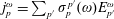
 $$\begin{eqnarray}\displaystyle & \displaystyle j_{sp}[\tilde{f}_{s}]=e_{s}\int _{-\infty }^{\infty }\text{d}v_{\Vert }\int _{0}^{\infty }\text{d}v_{\bot }\,v_{\bot }\int _{0}^{2\unicode[STIX]{x03C0}}\text{d}\unicode[STIX]{x1D711}\,v_{\Vert }^{1-|p|}\left(\frac{v_{\bot }}{\sqrt{2}}\right)^{|p|}\text{e}^{\text{i}p\unicode[STIX]{x1D711}}\,\tilde{f}_{s}, & \displaystyle\end{eqnarray}$$
 $$\begin{eqnarray}\displaystyle & \displaystyle \text{i}\frac{\unicode[STIX]{x2202}\tilde{f}_{s}}{\unicode[STIX]{x2202}t}=(k_{\bot }v_{\bot }\cos \unicode[STIX]{x1D711}+k_{\Vert }v_{\Vert })\tilde{f}_{s}+\text{i}\unicode[STIX]{x1D6FA}_{s}\frac{\unicode[STIX]{x2202}\tilde{f}_{s}}{\unicode[STIX]{x2202}\unicode[STIX]{x1D711}}+\frac{\text{i}e_{s}}{T_{s0}}f_{Ms}(v)\mathop{\sum }_{p}v_{\Vert }^{1-|p|}\left(\frac{v_{\bot }}{\sqrt{2}}\right)^{|p|}\text{e}^{-\text{i}p\unicode[STIX]{x1D711}}E_{p},\qquad & \displaystyle\end{eqnarray}$$
where the indices
 $p,p^{\prime }$
run through the ordered set
$p,p^{\prime }$
run through the ordered set
 $\{+,-,\Vert \}$
, with respectively assigned numerical values
$\{+,-,\Vert \}$
, with respectively assigned numerical values
 $\{+1,-1,0\}$
, and
$\{+1,-1,0\}$
, and
 $\unicode[STIX]{x1D705}_{p}^{p^{\prime }}$
is the representation of the operator
$\unicode[STIX]{x1D705}_{p}^{p^{\prime }}$
is the representation of the operator
 $-\text{i}\boldsymbol{k}\times$
in the unitary basis
$-\text{i}\boldsymbol{k}\times$
in the unitary basis
 $$\begin{eqnarray}\displaystyle \unicode[STIX]{x1D705}_{p}^{p^{\prime }}=\left(\begin{array}{@{}ccc@{}}k_{\Vert } & 0 & -k_{\bot }/\sqrt{2}\\ 0 & -k_{\Vert } & k_{\bot }/\sqrt{2}\\ -k_{\bot }/\sqrt{2} & k_{\bot }/\sqrt{2} & 0\end{array}\right). & & \displaystyle\end{eqnarray}$$
As expressed by (2.18)–(2.21), the linearized Vlasov–Maxwell system poses a three-dimensional problem in velocity space, the perturbed distribution functions depending on three velocity coordinates plus time:
 $\tilde{f}_{s}=\tilde{f}_{s}(v_{\Vert },v_{\bot },\unicode[STIX]{x1D711},t)$
. Since the dependence on the gyrophase coordinate
$\tilde{f}_{s}=\tilde{f}_{s}(v_{\Vert },v_{\bot },\unicode[STIX]{x1D711},t)$
. Since the dependence on the gyrophase coordinate
 $\unicode[STIX]{x1D711}$
is periodic, it can be analysed as a Fourier series. First, a change of dependent variables is carried out, from
$\unicode[STIX]{x1D711}$
is periodic, it can be analysed as a Fourier series. First, a change of dependent variables is carried out, from
 $\tilde{f}_{s}(v_{\Vert },v_{\bot },\unicode[STIX]{x1D711},t)$
to
$\tilde{f}_{s}(v_{\Vert },v_{\bot },\unicode[STIX]{x1D711},t)$
to
 $$\begin{eqnarray}\displaystyle \unicode[STIX]{x1D719}_{s}(v_{\Vert },v_{\bot },\unicode[STIX]{x1D711},t)=\tilde{f}_{s}(v_{\Vert },v_{\bot },\unicode[STIX]{x1D711},t)\,\exp \left(-\frac{\text{i}k_{\bot }v_{\bot }}{\unicode[STIX]{x1D6FA}_{s}}\sin \unicode[STIX]{x1D711}\right)=\tilde{f}_{s}\mathop{\sum }_{\ell =-\infty }^{\infty }\text{J}_{\ell }\left(\frac{k_{\bot }v_{\bot }}{\unicode[STIX]{x1D6FA}_{s}}\right)\text{e}^{-\text{i}\ell \unicode[STIX]{x1D711}}, & & \displaystyle \nonumber\\ \displaystyle & & \displaystyle\end{eqnarray}$$
where
 $\text{J}_{\ell }$
are the Bessel functions. Bringing this to (2.20) and (2.21), those equations become
$\text{J}_{\ell }$
are the Bessel functions. Bringing this to (2.20) and (2.21), those equations become
 $$\begin{eqnarray}\displaystyle j_{sp}[\unicode[STIX]{x1D719}_{s}]=e_{s}\int _{-\infty }^{\infty }\text{d}v_{\Vert }\int _{0}^{\infty }\text{d}v_{\bot }\,v_{\bot }\int _{0}^{2\unicode[STIX]{x03C0}}\text{d}\unicode[STIX]{x1D711}\,\mathop{\sum }_{\ell =-\infty }^{\infty }\text{J}_{\ell -p}\left(\frac{k_{\bot }v_{\bot }}{\unicode[STIX]{x1D6FA}_{s}}\right)v_{\Vert }^{1-|p|}\left(\frac{v_{\bot }}{\sqrt{2}}\right)^{|p|}\text{e}^{\text{i}\ell \unicode[STIX]{x1D711}}~\unicode[STIX]{x1D719}_{s} & & \displaystyle \nonumber\\ \displaystyle & & \displaystyle\end{eqnarray}$$
and
 $$\begin{eqnarray}\displaystyle \text{i}\frac{\unicode[STIX]{x2202}\unicode[STIX]{x1D719}_{s}}{\unicode[STIX]{x2202}t}=k_{\Vert }v_{\Vert }\unicode[STIX]{x1D719}_{s}+\text{i}\unicode[STIX]{x1D6FA}_{s}\frac{\unicode[STIX]{x2202}\unicode[STIX]{x1D719}_{s}}{\unicode[STIX]{x2202}\unicode[STIX]{x1D711}}+\frac{\text{i}e_{s}}{T_{s0}}f_{Ms}(v)\mathop{\sum }_{\ell p}\text{e}^{-\text{i}\ell \unicode[STIX]{x1D711}}\text{J}_{\ell -p}\left(\frac{k_{\bot }v_{\bot }}{\unicode[STIX]{x1D6FA}_{s}}\right)v_{\Vert }^{1-|p|}\left(\frac{v_{\bot }}{\sqrt{2}}\right)^{|p|}E_{p}.\quad & & \displaystyle\end{eqnarray}$$
The original distribution function
 $\tilde{f}_{s}$
is periodic in
$\tilde{f}_{s}$
is periodic in
 $\unicode[STIX]{x1D711}$
and the factor
$\unicode[STIX]{x1D711}$
and the factor
 $\exp (-\text{i}k_{\bot }v_{\bot }\sin \unicode[STIX]{x1D711}/\unicode[STIX]{x1D6FA}_{s})$
is also periodic. Therefore,
$\exp (-\text{i}k_{\bot }v_{\bot }\sin \unicode[STIX]{x1D711}/\unicode[STIX]{x1D6FA}_{s})$
is also periodic. Therefore,
 $\unicode[STIX]{x1D719}_{s}$
is a periodic function of
$\unicode[STIX]{x1D719}_{s}$
is a periodic function of
 $\unicode[STIX]{x1D711}$
and, defining
$\unicode[STIX]{x1D711}$
and, defining
 $$\begin{eqnarray}\displaystyle \unicode[STIX]{x1D719}_{sm}(v_{\Vert },v_{\bot },t)\equiv \frac{1}{2\unicode[STIX]{x03C0}}\int _{0}^{2\unicode[STIX]{x03C0}}\text{d}\unicode[STIX]{x1D711}\,\text{e}^{\text{i}m\unicode[STIX]{x1D711}}\unicode[STIX]{x1D719}_{s}(v_{\Vert },v_{\bot },\unicode[STIX]{x1D711},t) & & \displaystyle\end{eqnarray}$$
and
 $$\begin{eqnarray}\displaystyle h_{smp}(v_{\Vert },v_{\bot })\equiv \text{J}_{m-p}\left(\frac{k_{\bot }v_{\bot }}{\unicode[STIX]{x1D6FA}_{s}}\right)v_{\Vert }^{1-|p|}\left(\frac{v_{\bot }}{\sqrt{2}}\right)^{|p|}, & & \displaystyle\end{eqnarray}$$
where the index
 $s\in \{species\}$
runs through the set of plasma species,
$s\in \{species\}$
runs through the set of plasma species,
 $m\in \boldsymbol{Z}$
runs through the set of all integers and
$m\in \boldsymbol{Z}$
runs through the set of all integers and
 $p$
runs through the set
$p$
runs through the set
 $\{+,-,\Vert \}$
(or numerically
$\{+,-,\Vert \}$
(or numerically
 $\{+1,-1,0\}$
), equation (2.24) yields
$\{+1,-1,0\}$
), equation (2.24) yields
 $$\begin{eqnarray}\displaystyle j_{sp}[\unicode[STIX]{x1D719}_{sm}]=e_{s}\mathop{\sum }_{m=-\infty }^{\infty }\int \text{d}^{3}\boldsymbol{v}\,h_{smp}\,\unicode[STIX]{x1D719}_{sm} & & \displaystyle\end{eqnarray}$$
and (2.25) yields
 $$\begin{eqnarray}\displaystyle \text{i}\frac{\unicode[STIX]{x2202}\unicode[STIX]{x1D719}_{sm}}{\unicode[STIX]{x2202}t}=(k_{\Vert }v_{\Vert }+m\unicode[STIX]{x1D6FA}_{s})\unicode[STIX]{x1D719}_{sm}+\frac{\text{i}e_{s}}{T_{s0}}f_{Ms}(v)\mathop{\sum }_{p}h_{smp}\,E_{p}. & & \displaystyle\end{eqnarray}$$
In (2.28) and through the rest of the paper, when the integral operation
 $\int \text{d}^{3}\boldsymbol{v}$
acts on a function of
$\int \text{d}^{3}\boldsymbol{v}$
acts on a function of
 $(v_{\Vert },v_{\bot })$
, it is understood to be
$(v_{\Vert },v_{\bot })$
, it is understood to be
 $\int \text{d}^{3}\boldsymbol{v}=2\unicode[STIX]{x03C0}\int _{-\infty }^{\infty }\text{d}v_{\Vert }\int _{0}^{\infty }v_{\bot }\text{d}v_{\bot }$
.
$\int \text{d}^{3}\boldsymbol{v}=2\unicode[STIX]{x03C0}\int _{-\infty }^{\infty }\text{d}v_{\Vert }\int _{0}^{\infty }v_{\bot }\text{d}v_{\bot }$
.
The closed, linearized Vlasov–Maxwell system of (2.18), (2.19), (2.28), (2.29) can be written in compact form by defining the following state vector in two-dimensional
 $(v_{\Vert },v_{\bot })$
velocity space:
$(v_{\Vert },v_{\bot })$
velocity space:
 $$\begin{eqnarray}\displaystyle \unicode[STIX]{x1D713}(v_{\Vert },v_{\bot },t)\equiv \left(\begin{array}{@{}c@{}}E_{p}(t)\\ \tilde{B}_{p}(t)\\ \unicode[STIX]{x1D719}_{sm}(v_{\Vert },v_{\bot },t)\end{array}\right), & & \displaystyle\end{eqnarray}$$
whose time variation is governed by a first-order linear equation analogous to the Schrödinger equation of quantum mechanics,
 $$\begin{eqnarray}\displaystyle \text{i}\frac{\unicode[STIX]{x2202}\unicode[STIX]{x1D713}}{\unicode[STIX]{x2202}t}={\mathcal{H}}\unicode[STIX]{x1D713}, & & \displaystyle\end{eqnarray}$$
where the linear operator
 ${\mathcal{H}}$
is
${\mathcal{H}}$
is
 $$\begin{eqnarray}\displaystyle {\mathcal{H}}\left(\begin{array}{@{}c@{}}E_{p}\\ \tilde{B}_{p}\\ \unicode[STIX]{x1D719}_{sm}\end{array}\right)=\left(\begin{array}{@{}ccc@{}}0 & -\text{i}c^{2}\displaystyle \mathop{\sum }_{p^{\prime }}\unicode[STIX]{x1D705}_{p}^{p^{\prime }} & -\text{i}c^{2}\displaystyle \mathop{\sum }_{sm}e_{s}\displaystyle \int \text{d}^{3}\boldsymbol{v}\,h_{smp}\\ \text{i}\displaystyle \mathop{\sum }_{p^{\prime }}\unicode[STIX]{x1D705}_{p}^{p^{\prime }} & 0 & 0\\ \text{i}e_{s}T_{s0}^{-1}f_{Ms}\displaystyle \mathop{\sum }_{p^{\prime }}h_{smp^{\prime }} & 0 & k_{\Vert }v_{\Vert }+m\unicode[STIX]{x1D6FA}_{s}\end{array}\right)\left(\begin{array}{@{}c@{}}E_{p^{\prime }}\\ \tilde{B}_{p^{\prime }}\\ \unicode[STIX]{x1D719}_{sm}\end{array}\right). & & \displaystyle \nonumber\\ \displaystyle & & \displaystyle\end{eqnarray}$$
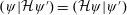
It will be shown next that, like the Hamiltonian in Schrödinger’s equation, the operator
 ${\mathcal{H}}$
is self-adjoint.
${\mathcal{H}}$
is self-adjoint.
3 Self-adjointness and formal solution of the initial-value problems
The above state vectors in two-dimensional
 $(v_{\Vert },v_{\bot })$
velocity space will be called two-dimensional (2-D) state vectors. The space of such 2-D state vectors can be given a Hilbert space structure by defining the scalar product
$(v_{\Vert },v_{\bot })$
velocity space will be called two-dimensional (2-D) state vectors. The space of such 2-D state vectors can be given a Hilbert space structure by defining the scalar product
 $$\begin{eqnarray}\displaystyle (\unicode[STIX]{x1D713}|\unicode[STIX]{x1D713}^{\prime })=\mathop{\sum }_{p}\left(\frac{1}{c^{2}}E_{p}^{\ast }E_{p}^{\prime }+\tilde{B}_{p}^{\ast }\tilde{B}_{p}^{\prime }\right)+\mathop{\sum }_{sm}\int \text{d}^{3}\boldsymbol{v}\,\frac{T_{s0}}{f_{Ms}(v)}\,\unicode[STIX]{x1D719}_{sm}^{\ast }(v_{\Vert },v_{\bot })\,\unicode[STIX]{x1D719}_{sm}^{\prime }(v_{\Vert },v_{\bot }). & & \displaystyle\end{eqnarray}$$
With this scalar product, the linear operator
 ${\mathcal{H}}$
(2.32) is self-adjoint because the product
${\mathcal{H}}$
(2.32) is self-adjoint because the product
 $(\unicode[STIX]{x1D713}|{\mathcal{H}}\unicode[STIX]{x1D713}^{\prime })$
can be cast in the Hermite-symmetric form
$(\unicode[STIX]{x1D713}|{\mathcal{H}}\unicode[STIX]{x1D713}^{\prime })$
can be cast in the Hermite-symmetric form
 $$\begin{eqnarray}\displaystyle (\unicode[STIX]{x1D713}|{\mathcal{H}}\unicode[STIX]{x1D713}^{\prime }) & = & \displaystyle \text{i}\mathop{\sum }_{pp^{\prime }}\unicode[STIX]{x1D705}_{p}^{p^{\prime }}(\tilde{B}_{p}^{\ast }E_{p^{\prime }}^{\prime }-E_{p}^{\ast }\tilde{B}_{p^{\prime }}^{\prime })+\text{i}\mathop{\sum }_{smp}e_{s}\int \text{d}^{3}\boldsymbol{v}\,h_{smp}\,(\unicode[STIX]{x1D719}_{sm}^{\ast }E_{p}^{\prime }-E_{p}^{\ast }\unicode[STIX]{x1D719}_{sm}^{\prime })\nonumber\\ \displaystyle & & \displaystyle +\,\mathop{\sum }_{sm}\int \text{d}^{3}\boldsymbol{v}\,\frac{T_{s0}}{f_{Ms}}\,(k_{\Vert }v_{\Vert }+m\unicode[STIX]{x1D6FA}_{s})\,\unicode[STIX]{x1D719}_{sm}^{\ast }\,\unicode[STIX]{x1D719}_{sm}^{\prime }.\end{eqnarray}$$
Since
 $h_{smp}$
is real and
$h_{smp}$
is real and
 $\unicode[STIX]{x1D705}_{p}^{p^{\prime }}$
is real and symmetric with respect to the
$\unicode[STIX]{x1D705}_{p}^{p^{\prime }}$
is real and symmetric with respect to the
 $p,p^{\prime }$
indices, this expression is invariant under the exchange of primed and unprimed variables followed by complex conjugation, hence
$p,p^{\prime }$
indices, this expression is invariant under the exchange of primed and unprimed variables followed by complex conjugation, hence
 $(\unicode[STIX]{x1D713}|{\mathcal{H}}\unicode[STIX]{x1D713}^{\prime })=({\mathcal{H}}\unicode[STIX]{x1D713}|\unicode[STIX]{x1D713}^{\prime })$
.
$(\unicode[STIX]{x1D713}|{\mathcal{H}}\unicode[STIX]{x1D713}^{\prime })=({\mathcal{H}}\unicode[STIX]{x1D713}|\unicode[STIX]{x1D713}^{\prime })$
.
From its time evolution equation (2.31), the dynamical solution for
 $\unicode[STIX]{x1D713}(v_{\Vert },v_{\bot },t)$
satisfying the initial condition
$\unicode[STIX]{x1D713}(v_{\Vert },v_{\bot },t)$
satisfying the initial condition
 $\unicode[STIX]{x1D713}(v_{\Vert },v_{\bot },0)$
is
$\unicode[STIX]{x1D713}(v_{\Vert },v_{\bot },0)$
is
 $$\begin{eqnarray}\displaystyle \unicode[STIX]{x1D713}(v_{\Vert },v_{\bot },t)=\exp (-\text{i}t{\mathcal{H}})\,\unicode[STIX]{x1D713}(v_{\Vert },v_{\bot },0). & & \displaystyle\end{eqnarray}$$
This solution is applicable both to positive and negative times. Since
 ${\mathcal{H}}$
is a Hermitian operator and
${\mathcal{H}}$
is a Hermitian operator and
 $t$
is a real variable,
$t$
is a real variable,
 $\exp (-\text{i}t{\mathcal{H}})$
is a unitary operator, therefore the state vector norm
$\exp (-\text{i}t{\mathcal{H}})$
is a unitary operator, therefore the state vector norm
 $$\begin{eqnarray}\displaystyle (\unicode[STIX]{x1D713}|\unicode[STIX]{x1D713}) & = & \displaystyle \left(\frac{1}{c^{2}}\boldsymbol{E}^{\ast }\boldsymbol{\cdot }\boldsymbol{E}+\tilde{\boldsymbol{B}}^{\ast }\boldsymbol{\cdot }\tilde{\boldsymbol{B}}\right)(t)+\mathop{\sum }_{sm}\int \text{d}^{3}\boldsymbol{v}\,\frac{T_{s0}}{f_{Ms}(v)}~\unicode[STIX]{x1D719}_{sm}^{\ast }(v_{\Vert },v_{\bot },t)\,\unicode[STIX]{x1D719}_{sm}(v_{\Vert },v_{\bot },t)\nonumber\\ \displaystyle & = & \displaystyle \left(\frac{1}{c^{2}}\boldsymbol{E}^{\ast }\boldsymbol{\cdot }\boldsymbol{E}+\tilde{\boldsymbol{B}}^{\ast }\boldsymbol{\cdot }\tilde{\boldsymbol{B}}\right)(t)+\mathop{\sum }_{s}\int \text{d}^{3}\boldsymbol{v}\,\frac{T_{s0}}{f_{Ms}(v)}\,\tilde{f}_{s}^{\ast }(v_{\Vert },v_{\bot },\unicode[STIX]{x1D711},t)\,\tilde{f}_{s}(v_{\Vert },v_{\bot },\unicode[STIX]{x1D711},t)\nonumber\\ \displaystyle & & \displaystyle\end{eqnarray}$$
is independent of time. This norm has the physical interpretation that it equals twice the quadratic contribution of the considered
 $\boldsymbol{k}$
-mode to the free energy,
$\boldsymbol{k}$
-mode to the free energy,
 ${\mathcal{E}}-\sum _{s}T_{s0}{\mathcal{S}}_{s}$
, where
${\mathcal{E}}-\sum _{s}T_{s0}{\mathcal{S}}_{s}$
, where
 ${\mathcal{E}}$
is the conserved total energy of the perturbation and
${\mathcal{E}}$
is the conserved total energy of the perturbation and
 ${\mathcal{S}}_{s}$
are the conserved entropies of each species. The conservation of such a norm implies that the Maxwellian equilibrium is linearly stable, as was first shown by Newcomb and reported in the appendix of Bernstein (Reference Bernstein1958).
${\mathcal{S}}_{s}$
are the conserved entropies of each species. The conservation of such a norm implies that the Maxwellian equilibrium is linearly stable, as was first shown by Newcomb and reported in the appendix of Bernstein (Reference Bernstein1958).
Another important consequence of the self-adjointness of
 ${\mathcal{H}}$
is the existence of a complete basis made of normal modes, that spans the whole Hilbert space of 2-D state vectors. These normal modes are separable solutions of (2.31) having the form
${\mathcal{H}}$
is the existence of a complete basis made of normal modes, that spans the whole Hilbert space of 2-D state vectors. These normal modes are separable solutions of (2.31) having the form
 $$\begin{eqnarray}\displaystyle \unicode[STIX]{x1D713}(v_{\Vert },v_{\bot },t)=\unicode[STIX]{x1D713}^{\unicode[STIX]{x1D714},\unicode[STIX]{x1D708}}(v_{\Vert },v_{\bot })\,\text{e}^{-\text{i}\unicode[STIX]{x1D714}t}, & & \displaystyle\end{eqnarray}$$
hence
 $\unicode[STIX]{x1D713}^{\unicode[STIX]{x1D714},\unicode[STIX]{x1D708}}$
is an eigenfunction of the operator
$\unicode[STIX]{x1D713}^{\unicode[STIX]{x1D714},\unicode[STIX]{x1D708}}$
is an eigenfunction of the operator
 ${\mathcal{H}}$
with eigenvalue
${\mathcal{H}}$
with eigenvalue
 $\unicode[STIX]{x1D714}$
 $$\begin{eqnarray}\displaystyle {\mathcal{H}}\unicode[STIX]{x1D713}^{\unicode[STIX]{x1D714},\unicode[STIX]{x1D708}}=\unicode[STIX]{x1D714}\,\unicode[STIX]{x1D713}^{\unicode[STIX]{x1D714},\unicode[STIX]{x1D708}} & & \displaystyle\end{eqnarray}$$
and, again as the consequence of
 ${\mathcal{H}}$
being self-adjoint, the spectrum of normal-mode eigenfrequencies
${\mathcal{H}}$
being self-adjoint, the spectrum of normal-mode eigenfrequencies
 $\unicode[STIX]{x1D714}$
is real. The additional index
$\unicode[STIX]{x1D714}$
is real. The additional index
 $\unicode[STIX]{x1D708}$
is meant to label generically the different independent eigenfunctions that can have the same eigenvalue
$\unicode[STIX]{x1D708}$
is meant to label generically the different independent eigenfunctions that can have the same eigenvalue
 $\unicode[STIX]{x1D714}$
when the latter is degenerate. Since the set of normal modes forms a complete basis for the Hilbert space of state vectors, any initial condition belonging to such space can be expanded as
$\unicode[STIX]{x1D714}$
when the latter is degenerate. Since the set of normal modes forms a complete basis for the Hilbert space of state vectors, any initial condition belonging to such space can be expanded as
 $$\begin{eqnarray}\displaystyle \unicode[STIX]{x1D713}(v_{\Vert },v_{\bot },0)=\widehat{\mathop{\sum }_{\unicode[STIX]{x1D714},\unicode[STIX]{x1D708}}}\,c_{\unicode[STIX]{x1D714},\unicode[STIX]{x1D708}}\,\unicode[STIX]{x1D713}^{\unicode[STIX]{x1D714},\unicode[STIX]{x1D708}}(v_{\Vert },v_{\bot }), & & \displaystyle\end{eqnarray}$$
where
 $\widehat{\sum _{\unicode[STIX]{x1D714},\unicode[STIX]{x1D708}}}$
indicates a sum if the index runs through a set of discrete values and an integral if the index runs through a continuum. Then, the solution for
$\widehat{\sum _{\unicode[STIX]{x1D714},\unicode[STIX]{x1D708}}}$
indicates a sum if the index runs through a set of discrete values and an integral if the index runs through a continuum. Then, the solution for
 $\unicode[STIX]{x1D713}(v_{\Vert },v_{\bot },t)$
(3.3) is simply
$\unicode[STIX]{x1D713}(v_{\Vert },v_{\bot },t)$
(3.3) is simply
 $$\begin{eqnarray}\displaystyle \unicode[STIX]{x1D713}(v_{\Vert },v_{\bot },t)=\widehat{\mathop{\sum }_{\unicode[STIX]{x1D714},\unicode[STIX]{x1D708}}}\,c_{\unicode[STIX]{x1D714},\unicode[STIX]{x1D708}}\,\unicode[STIX]{x1D713}^{\unicode[STIX]{x1D714},\unicode[STIX]{x1D708}}(v_{\Vert },v_{\bot })\,\text{e}^{-\text{i}\unicode[STIX]{x1D714}t}. & & \displaystyle\end{eqnarray}$$
So, the solution of any initial-value problem would be immediate if the complete set of eigenfunctions of the operator
 ${\mathcal{H}}$
were available. The following sections will be devoted to the investigation of such normal-mode eigenfunctions. This requires separate consideration of the case of a wavevector not perpendicular to the equilibrium magnetic field (
${\mathcal{H}}$
were available. The following sections will be devoted to the investigation of such normal-mode eigenfunctions. This requires separate consideration of the case of a wavevector not perpendicular to the equilibrium magnetic field (
 $k_{\Vert }\not =0$
) from the
$k_{\Vert }\not =0$
) from the
 $k_{\Vert }=0$
case of wave propagation perpendicular to the equilibrium magnetic field.
$k_{\Vert }=0$
case of wave propagation perpendicular to the equilibrium magnetic field.
4 Continuum of singular 2-D normal modes for
 $k_{\Vert }\not =0$

When
 $k_{\Vert }\not =0$
, the spectrum of normal-mode eigenfrequencies covers the set of real numbers
$k_{\Vert }\not =0$
, the spectrum of normal-mode eigenfrequencies covers the set of real numbers
 $\boldsymbol{R}$
. The eigenfunctions of this continuous spectrum are singular (they are distributions in the mathematical sense that lie outside the Hilbert space of normalizable state vectors) and the eigenvalues
$\boldsymbol{R}$
. The eigenfunctions of this continuous spectrum are singular (they are distributions in the mathematical sense that lie outside the Hilbert space of normalizable state vectors) and the eigenvalues
 $\unicode[STIX]{x1D714}\in \boldsymbol{R}$
are highly degenerate. In order to show this, consider the normal-mode system (2.32) for one such eigenfunction satisfying
$\unicode[STIX]{x1D714}\in \boldsymbol{R}$
are highly degenerate. In order to show this, consider the normal-mode system (2.32) for one such eigenfunction satisfying
 ${\mathcal{H}}\unicode[STIX]{x1D713}^{\unicode[STIX]{x1D714}}=\unicode[STIX]{x1D714}\unicode[STIX]{x1D713}^{\unicode[STIX]{x1D714}}$
 $$\begin{eqnarray}\displaystyle & \displaystyle \unicode[STIX]{x1D714}E_{p}^{\unicode[STIX]{x1D714}}=-\text{i}c^{2}\mathop{\sum }_{p^{\prime }}\unicode[STIX]{x1D705}_{p}^{p^{\prime }}\tilde{B}_{p^{\prime }}^{\unicode[STIX]{x1D714}}\,-\text{i}c^{2}\mathop{\sum }_{sm}e_{s}\int \text{d}^{3}\boldsymbol{v}\,h_{smp}\,\unicode[STIX]{x1D719}_{sm}^{\unicode[STIX]{x1D714}} & \displaystyle\end{eqnarray}$$
 $$\begin{eqnarray}\displaystyle & \displaystyle \unicode[STIX]{x1D714}\tilde{B}_{p}^{\unicode[STIX]{x1D714}}=\text{i}\mathop{\sum }_{p^{\prime }}\unicode[STIX]{x1D705}_{p}^{p^{\prime }}E_{p^{\prime }}^{\unicode[STIX]{x1D714}} & \displaystyle\end{eqnarray}$$
 $$\begin{eqnarray}\displaystyle & \displaystyle (\unicode[STIX]{x1D714}-k_{\Vert }v_{\Vert }-m\unicode[STIX]{x1D6FA}_{s})\unicode[STIX]{x1D719}_{sm}^{\unicode[STIX]{x1D714}}=\text{i}e_{s}T_{s0}^{-1}f_{Ms}\mathop{\sum }_{p^{\prime }}h_{smp^{\prime }}E_{p^{\prime }}^{\unicode[STIX]{x1D714}}. & \displaystyle\end{eqnarray}$$
Eliminating
 $\tilde{B}_{p}^{\unicode[STIX]{x1D714}}$
, equations (4.1), (4.2) yield
$\tilde{B}_{p}^{\unicode[STIX]{x1D714}}$
, equations (4.1), (4.2) yield
 $$\begin{eqnarray}\displaystyle \mathop{\sum }_{p^{\prime }}\left[\unicode[STIX]{x1D6FF}_{p}^{p^{\prime }}-\frac{c^{2}}{\unicode[STIX]{x1D714}^{2}}(\unicode[STIX]{x1D705}^{2})_{p}^{p^{\prime }}\right]E_{p^{\prime }}^{\unicode[STIX]{x1D714}}+\frac{\text{i}c^{2}}{\unicode[STIX]{x1D714}}\mathop{\sum }_{sm}e_{s}\int \text{d}^{3}\boldsymbol{v}\,h_{smp}\,\unicode[STIX]{x1D719}_{sm}^{\unicode[STIX]{x1D714}}=0, & & \displaystyle\end{eqnarray}$$
where
 $\unicode[STIX]{x1D6FF}_{p}^{p^{\prime }}$
is the Kronecker delta and
$\unicode[STIX]{x1D6FF}_{p}^{p^{\prime }}$
is the Kronecker delta and
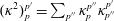 $(\unicode[STIX]{x1D705}^{2})_{p}^{p^{\prime }}=\sum _{p^{\prime \prime }}\unicode[STIX]{x1D705}_{p}^{p^{\prime \prime }}\unicode[STIX]{x1D705}_{p^{\prime \prime }}^{p^{\prime }}$
is the representation of the operator
$(\unicode[STIX]{x1D705}^{2})_{p}^{p^{\prime }}=\sum _{p^{\prime \prime }}\unicode[STIX]{x1D705}_{p}^{p^{\prime \prime }}\unicode[STIX]{x1D705}_{p^{\prime \prime }}^{p^{\prime }}$
is the representation of the operator
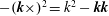 $-(\boldsymbol{k}\times )^{2}=k^{2}-\boldsymbol{k}\boldsymbol{k}$
in the unitary basis,
$-(\boldsymbol{k}\times )^{2}=k^{2}-\boldsymbol{k}\boldsymbol{k}$
in the unitary basis,
 $$\begin{eqnarray}\displaystyle (\unicode[STIX]{x1D705}^{2})_{p}^{p^{\prime }}=\left(\begin{array}{@{}ccc@{}}k_{\Vert }^{2}+k_{\bot }^{2}/2 & -k_{\bot }^{2}/2 & -k_{\Vert }k_{\bot }/\sqrt{2}\\ -k_{\bot }^{2}/2 & k_{\Vert }^{2}+k_{\bot }^{2}/2 & -k_{\Vert }k_{\bot }/\sqrt{2}\\ -k_{\Vert }k_{\bot }/\sqrt{2} & -k_{\Vert }k_{\bot }/\sqrt{2} & k_{\bot }^{2}\end{array}\right). & & \displaystyle\end{eqnarray}$$
For
 $k_{\Vert }\not =0$
and any real
$k_{\Vert }\not =0$
and any real
 $\unicode[STIX]{x1D714}$
, equation (4.3) has the general solution
$\unicode[STIX]{x1D714}$
, equation (4.3) has the general solution
 $$\begin{eqnarray}\displaystyle \unicode[STIX]{x1D719}_{sm}^{\unicode[STIX]{x1D714}}(v_{\Vert },v_{\bot })=\frac{\text{i}e_{s}}{T_{s0}}\mathop{\sum }_{p^{\prime }}{\mathcal{P}}\frac{f_{Ms}(v)\,h_{smp^{\prime }}(v_{\Vert },v_{\bot })}{\unicode[STIX]{x1D714}-k_{\Vert }v_{\Vert }-m\unicode[STIX]{x1D6FA}_{s}}\,E_{p^{\prime }}^{\unicode[STIX]{x1D714}}+\frac{\text{i}\unicode[STIX]{x1D714}}{2\unicode[STIX]{x03C0}c^{2}e_{s}}\,\unicode[STIX]{x1D706}_{sm}^{\unicode[STIX]{x1D714}}(v_{\bot })\,\unicode[STIX]{x1D6FF}(v_{\Vert }-v_{sm}^{\unicode[STIX]{x1D714}}), & & \displaystyle\end{eqnarray}$$
where
 ${\mathcal{P}}$
stands for the Cauchy principal value,
${\mathcal{P}}$
stands for the Cauchy principal value,
 $\unicode[STIX]{x1D6FF}$
is the Dirac distribution,
$\unicode[STIX]{x1D6FF}$
is the Dirac distribution,
 $v_{sm}^{\unicode[STIX]{x1D714}}\equiv (\unicode[STIX]{x1D714}-m\unicode[STIX]{x1D6FA}_{s})/k_{\Vert }$
and the functions
$v_{sm}^{\unicode[STIX]{x1D714}}\equiv (\unicode[STIX]{x1D714}-m\unicode[STIX]{x1D6FA}_{s})/k_{\Vert }$
and the functions
 $\unicode[STIX]{x1D706}_{sm}^{\unicode[STIX]{x1D714}}(v_{\bot })$
are arbitrary. Substituting this solution for
$\unicode[STIX]{x1D706}_{sm}^{\unicode[STIX]{x1D714}}(v_{\bot })$
are arbitrary. Substituting this solution for
 $\unicode[STIX]{x1D719}_{sm}^{\unicode[STIX]{x1D714}}$
in (4.4), one gets the final condition
$\unicode[STIX]{x1D719}_{sm}^{\unicode[STIX]{x1D714}}$
in (4.4), one gets the final condition
 $$\begin{eqnarray}\displaystyle \mathop{\sum }_{p^{\prime }}\unicode[STIX]{x1D717}_{p}^{p^{\prime }}(\unicode[STIX]{x1D714})\,E_{p^{\prime }}^{\unicode[STIX]{x1D714}}-\mathop{\sum }_{sm}\int _{0}^{\infty }\text{d}v_{\bot }\,v_{\bot }\,\unicode[STIX]{x1D706}_{sm}^{\unicode[STIX]{x1D714}}(v_{\bot })\,h_{smp}(v_{sm}^{\unicode[STIX]{x1D714}},v_{\bot })=0, & & \displaystyle\end{eqnarray}$$
where, for the real eigenfrequencies under consideration,
 $\unicode[STIX]{x1D717}_{p}^{p^{\prime }}(\unicode[STIX]{x1D714})$
is the real and symmetric tensor
$\unicode[STIX]{x1D717}_{p}^{p^{\prime }}(\unicode[STIX]{x1D714})$
is the real and symmetric tensor
 $$\begin{eqnarray}\displaystyle \unicode[STIX]{x1D717}_{p}^{p^{\prime }}(\unicode[STIX]{x1D714})\equiv \unicode[STIX]{x1D6FF}_{p}^{p^{\prime }}-\frac{c^{2}}{\unicode[STIX]{x1D714}^{2}}(\unicode[STIX]{x1D705}^{2})_{p}^{p^{\prime }}-\mathop{\sum }_{sm}\frac{c^{2}e_{s}^{2}}{\unicode[STIX]{x1D714}T_{s0}}\int \,\text{d}^{3}\boldsymbol{v}\,{\mathcal{P}}\frac{f_{Ms}(v)\,h_{smp}(v_{\Vert },v_{\bot })\,h_{smp^{\prime }}(v_{\Vert },v_{\bot })}{\unicode[STIX]{x1D714}-k_{\Vert }v_{\Vert }-m\unicode[STIX]{x1D6FA}_{s}}, & & \displaystyle\end{eqnarray}$$
which depends only on the frequency, plus the wavevector and equilibrium parameters. Since the form of the functions
 $\unicode[STIX]{x1D706}_{sm}^{\unicode[STIX]{x1D714}}(v_{\bot })$
is arbitrary in principle and (4.7) is just a set of three integral constraints, a large class of independent
$\unicode[STIX]{x1D706}_{sm}^{\unicode[STIX]{x1D714}}(v_{\bot })$
is arbitrary in principle and (4.7) is just a set of three integral constraints, a large class of independent
 $\unicode[STIX]{x1D706}_{sm}^{\unicode[STIX]{x1D714}}(v_{\bot })$
solutions exists for each real
$\unicode[STIX]{x1D706}_{sm}^{\unicode[STIX]{x1D714}}(v_{\bot })$
solutions exists for each real
 $\unicode[STIX]{x1D714}$
. The precise identification of all of them is difficult and impractical. However, this will not be necessary and, for the purposes of this work, all that will be needed is the general classification of the normal-mode solutions into three broad categories as described in appendix A.
$\unicode[STIX]{x1D714}$
. The precise identification of all of them is difficult and impractical. However, this will not be necessary and, for the purposes of this work, all that will be needed is the general classification of the normal-mode solutions into three broad categories as described in appendix A.
Notice that (4.7), (4.8) are the expression of Maxwell’s equation for the normal modes
 $$\begin{eqnarray}\displaystyle \mathop{\sum }_{p^{\prime }}\left[\unicode[STIX]{x1D6FF}_{p}^{p^{\prime }}-\frac{c^{2}}{\unicode[STIX]{x1D714}^{2}}(\unicode[STIX]{x1D705}^{2})_{p}^{p^{\prime }}\right]E_{p^{\prime }}^{\unicode[STIX]{x1D714}}+\frac{\text{i}c^{2}}{\unicode[STIX]{x1D714}}j_{p}^{\unicode[STIX]{x1D714}}=0, & & \displaystyle\end{eqnarray}$$
where
 $j_{p}^{\unicode[STIX]{x1D714}}=\sum _{s}j_{sp}^{\unicode[STIX]{x1D714}}$
is the total electric current. It is customary to express this current as the action of a conductivity tensor on the electric field,
$j_{p}^{\unicode[STIX]{x1D714}}=\sum _{s}j_{sp}^{\unicode[STIX]{x1D714}}$
is the total electric current. It is customary to express this current as the action of a conductivity tensor on the electric field,
 $j_{p}^{\unicode[STIX]{x1D714}}=\sum _{p^{\prime }}\unicode[STIX]{x1D70E}_{p}^{p^{\prime }}(\unicode[STIX]{x1D714})E_{p^{\prime }}^{\unicode[STIX]{x1D714}}$
. For some theories (and also in the special
$j_{p}^{\unicode[STIX]{x1D714}}=\sum _{p^{\prime }}\unicode[STIX]{x1D70E}_{p}^{p^{\prime }}(\unicode[STIX]{x1D714})E_{p^{\prime }}^{\unicode[STIX]{x1D714}}$
. For some theories (and also in the special
 $k_{\Vert }=0$
case of the present theory to be discussed in § 8), such conductivity tensor can be determined a priori as an intrinsic property of the plasma equilibrium for each mode wavenumber and frequency. Then, the normal-mode problem reduces to solving a dispersion relation, with the normal-mode electric field as the corresponding non-trivial eigenvector in the null space of the dispersion tensor. This is not true for the present theory in the
$k_{\Vert }=0$
case of the present theory to be discussed in § 8), such conductivity tensor can be determined a priori as an intrinsic property of the plasma equilibrium for each mode wavenumber and frequency. Then, the normal-mode problem reduces to solving a dispersion relation, with the normal-mode electric field as the corresponding non-trivial eigenvector in the null space of the dispersion tensor. This is not true for the present theory in the
 $k_{\Vert }\not =0$
case being considered now. For the present
$k_{\Vert }\not =0$
case being considered now. For the present
 $k_{\Vert }\not =0$
normal modes (4.7), (4.8), a part of the current can be represented as the action of an intrinsic conductivity tensor on the electric field and this has been included as the last term of the tensor
$k_{\Vert }\not =0$
normal modes (4.7), (4.8), a part of the current can be represented as the action of an intrinsic conductivity tensor on the electric field and this has been included as the last term of the tensor
 $\unicode[STIX]{x1D717}_{p}^{p^{\prime }}(\unicode[STIX]{x1D714})$
defined in (4.8). However, the part of the current given by the second term of the left-hand side of (4.7) depends on the eigenvector solution for
$\unicode[STIX]{x1D717}_{p}^{p^{\prime }}(\unicode[STIX]{x1D714})$
defined in (4.8). However, the part of the current given by the second term of the left-hand side of (4.7) depends on the eigenvector solution for
 $\unicode[STIX]{x1D706}_{sm}^{\unicode[STIX]{x1D714}}(v_{\bot })$
and can be related to the electric field only after such a solution has been specified. Therefore, for the present
$\unicode[STIX]{x1D706}_{sm}^{\unicode[STIX]{x1D714}}(v_{\bot })$
and can be related to the electric field only after such a solution has been specified. Therefore, for the present
 $k_{\Vert }\not =0$
normal modes, one can only write
$k_{\Vert }\not =0$
normal modes, one can only write
 $$\begin{eqnarray}\displaystyle j_{p}^{\unicode[STIX]{x1D714}}=\mathop{\sum }_{p^{\prime }}[\unicode[STIX]{x1D70E}_{H,p}^{p^{\prime }}(\unicode[STIX]{x1D714})+\unicode[STIX]{x1D70E}_{N,p}^{p^{\prime }}(\unicode[STIX]{x1D714};\unicode[STIX]{x1D706}_{sm}^{\unicode[STIX]{x1D714}})]E_{p^{\prime }}^{\unicode[STIX]{x1D714}}, & & \displaystyle\end{eqnarray}$$
where
 $\unicode[STIX]{x1D70E}_{H,p}^{p^{\prime }}(\unicode[STIX]{x1D714})$
is the intrinsic part of the conductivity tensor represented by the last term of (4.8),
$\unicode[STIX]{x1D70E}_{H,p}^{p^{\prime }}(\unicode[STIX]{x1D714})$
is the intrinsic part of the conductivity tensor represented by the last term of (4.8),
 $$\begin{eqnarray}\displaystyle \unicode[STIX]{x1D70E}_{H,p}^{p^{\prime }}(\unicode[STIX]{x1D714})=\mathop{\sum }_{sm}\frac{\text{i}e_{s}^{2}}{T_{s0}}\int \,\text{d}^{3}\boldsymbol{v}\,{\mathcal{P}}\frac{f_{Ms}(v)\,h_{smp}(v_{\Vert },v_{\bot })\,h_{smp^{\prime }}(v_{\Vert },v_{\bot })}{\unicode[STIX]{x1D714}-k_{\Vert }v_{\Vert }-m\unicode[STIX]{x1D6FA}_{s}}, & & \displaystyle\end{eqnarray}$$
and
 $\unicode[STIX]{x1D70E}_{N,p}^{p^{\prime }}(\unicode[STIX]{x1D714};\unicode[STIX]{x1D706}_{sm}^{\unicode[STIX]{x1D714}})$
is the non-intrinsic part that corresponds to the part of the current given by the second term of the left-hand side of (4.7). Since this non-intrinsic part can only be determined after the normal-mode solution has been obtained, the conductivity tensor concept is not useful here. Nevertheless, one can always evaluate the intrinsic part (4.11) which is a standard calculation found in the traditional plasma wave literature, more often expressed in Cartesian coordinates (see e.g. Brambilla Reference Brambilla1998). After integrating over
$\unicode[STIX]{x1D70E}_{N,p}^{p^{\prime }}(\unicode[STIX]{x1D714};\unicode[STIX]{x1D706}_{sm}^{\unicode[STIX]{x1D714}})$
is the non-intrinsic part that corresponds to the part of the current given by the second term of the left-hand side of (4.7). Since this non-intrinsic part can only be determined after the normal-mode solution has been obtained, the conductivity tensor concept is not useful here. Nevertheless, one can always evaluate the intrinsic part (4.11) which is a standard calculation found in the traditional plasma wave literature, more often expressed in Cartesian coordinates (see e.g. Brambilla Reference Brambilla1998). After integrating over
 $v_{\bot }$
, one gets
$v_{\bot }$
, one gets
 $$\begin{eqnarray}\displaystyle \unicode[STIX]{x1D70E}_{H,p}^{p^{\prime }}(\unicode[STIX]{x1D714})=\mathop{\sum }_{sm}\frac{\text{i}\unicode[STIX]{x1D714}_{Ps}^{2}}{c^{2}}\int _{-\infty }^{\infty }\text{d}v_{\Vert }\,{\mathcal{P}}\frac{F_{Ms}(v_{\Vert })\,[\unicode[STIX]{x1D6FC}_{sm}(v_{\Vert })]_{p}^{p^{\prime }}}{n_{s0}\,(\unicode[STIX]{x1D714}-k_{\Vert }v_{\Vert }-m\unicode[STIX]{x1D6FA}_{s})}, & & \displaystyle\end{eqnarray}$$
where
 $\unicode[STIX]{x1D714}_{Ps}^{2}\equiv c^{2}e_{s}^{2}n_{s0}/m_{s}$
is the squared plasma frequency of the species
$\unicode[STIX]{x1D714}_{Ps}^{2}\equiv c^{2}e_{s}^{2}n_{s0}/m_{s}$
is the squared plasma frequency of the species
 $s$
,
$s$
,
 $F_{Ms}(v_{\Vert })$
is the 1-D Maxwellian distribution function
$F_{Ms}(v_{\Vert })$
is the 1-D Maxwellian distribution function
 $$\begin{eqnarray}\displaystyle F_{Ms}(v_{\Vert })\equiv 2\unicode[STIX]{x03C0}\int _{0}^{\infty }\text{d}v_{\bot }\,v_{\bot }\,f_{Ms}(v)=\frac{n_{s0}}{(2\unicode[STIX]{x03C0})^{1/2}v_{ths}}\exp \left(-\frac{v_{\Vert }^{2}}{2v_{ths}^{2}}\right) & & \displaystyle\end{eqnarray}$$
and
 $$\begin{eqnarray}\displaystyle [\unicode[STIX]{x1D6FC}_{sm}(v_{\Vert })]_{p}^{p^{\prime }}\equiv \frac{1}{v_{ths}^{4}}\int _{0}^{\infty }\text{d}v_{\bot }\,v_{\bot }\exp \left(-\frac{v_{\bot }^{2}}{2v_{ths}^{2}}\right)h_{smp}(v_{\Vert },v_{\bot })\,h_{smp^{\prime }}(v_{\Vert },v_{\bot }), & & \displaystyle\end{eqnarray}$$
with the explicit result
 $$\begin{eqnarray}\displaystyle & \displaystyle [\unicode[STIX]{x1D6FC}_{sm}]_{+}^{+}=\text{e}^{-b_{s}}[b_{s}\text{I}_{m}(b_{s})-(b_{s}-m)\text{I}_{m-1}(b_{s})] & \displaystyle\end{eqnarray}$$
 $$\begin{eqnarray}\displaystyle & \displaystyle [\unicode[STIX]{x1D6FC}_{sm}]_{-}^{+}=[\unicode[STIX]{x1D6FC}_{sm}]_{+}^{-}=\frac{b_{s}}{2}\text{e}^{-b_{s}}[\text{I}_{m+1}(b_{s})+\text{I}_{m-1}(b_{s})-2\text{I}_{m}(b_{s})] & \displaystyle\end{eqnarray}$$
 $$\begin{eqnarray}\displaystyle & \displaystyle [\unicode[STIX]{x1D6FC}_{sm}]_{-}^{-}=\text{e}^{-b_{s}}[b_{s}\text{I}_{m}(b_{s})-(b_{s}+m)\text{I}_{m+1}(b_{s})] & \displaystyle\end{eqnarray}$$
 $$\begin{eqnarray}\displaystyle & \displaystyle [\unicode[STIX]{x1D6FC}_{sm}(v_{\Vert })]_{\Vert }^{+}=[\unicode[STIX]{x1D6FC}_{sm}(v_{\Vert })]_{+}^{\Vert }=\frac{v_{\Vert }\,b_{s}}{\sqrt{2}\,v_{ths}}~\text{e}^{-b_{s}}[\text{I}_{m-1}(b_{s})-\text{I}_{m}(b_{s})] & \displaystyle\end{eqnarray}$$
 $$\begin{eqnarray}\displaystyle & \displaystyle [\unicode[STIX]{x1D6FC}_{sm}(v_{\Vert })]_{\Vert }^{-}=[\unicode[STIX]{x1D6FC}_{sm}(v_{\Vert })]_{-}^{\Vert }=\frac{v_{\Vert }\,b_{s}}{\sqrt{2}\,v_{ths}}\,\text{e}^{-b_{s}}[\text{I}_{m}(b_{s})-\text{I}_{m+1}(b_{s})] & \displaystyle\end{eqnarray}$$
 $$\begin{eqnarray}\displaystyle & \displaystyle [\unicode[STIX]{x1D6FC}_{sm}(v_{\Vert })]_{\Vert }^{\Vert }=\frac{v_{\Vert }^{2}}{v_{ths}^{2}}\,\text{e}^{-b_{s}}\text{I}_{m}(b_{s}), & \displaystyle\end{eqnarray}$$
where
 $\text{I}_{m}$
are the modified Bessel functions and
$\text{I}_{m}$
are the modified Bessel functions and
 $b_{s}\equiv (k_{\bot }v_{ths}/\unicode[STIX]{x1D6FA}_{s})^{2}$
. Then, the results of the integrals over
$b_{s}\equiv (k_{\bot }v_{ths}/\unicode[STIX]{x1D6FA}_{s})^{2}$
. Then, the results of the integrals over
 $v_{\Vert }$
in (4.12) are given in terms of the real part of the plasma dispersion function
$v_{\Vert }$
in (4.12) are given in terms of the real part of the plasma dispersion function
 $Z$
(Fried & Conte Reference Fried and Conte1961)
.
$Z$
(Fried & Conte Reference Fried and Conte1961)
.
The determinant of the
 $3\times 3$
matrix
$3\times 3$
matrix
 $[\unicode[STIX]{x1D6FC}_{sm}(v_{\Vert })]_{p}^{p^{\prime }}$
with indices
$[\unicode[STIX]{x1D6FC}_{sm}(v_{\Vert })]_{p}^{p^{\prime }}$
with indices
 $p,p^{\prime }$
is
$p,p^{\prime }$
is
 $$\begin{eqnarray}\displaystyle \text{det}[\unicode[STIX]{x1D6FC}_{sm}(v_{\Vert })]=\frac{v_{\Vert }^{2}}{v_{ths}^{2}}\,\text{e}^{-3b_{s}}\,m^{2}(1-b_{s})\text{I}_{m}(b_{s})[\text{I}_{m}^{2}(b_{s})-\text{I}_{m+1}(b_{s})\text{I}_{m-1}(b_{s})]. & & \displaystyle\end{eqnarray}$$
Therefore, the inverse matrix
 $[\unicode[STIX]{x1D6FC}_{sm}^{-1}]_{p}^{p^{\prime }}$
such that
$[\unicode[STIX]{x1D6FC}_{sm}^{-1}]_{p}^{p^{\prime }}$
such that
 $\sum _{p^{\prime \prime }}[\unicode[STIX]{x1D6FC}_{sm}^{-1}]_{p}^{p^{\prime \prime }}[\unicode[STIX]{x1D6FC}_{sm}]_{p^{\prime \prime }}^{p^{\prime }}=\unicode[STIX]{x1D6FF}_{p}^{p^{\prime }}$
exists except for
$\sum _{p^{\prime \prime }}[\unicode[STIX]{x1D6FC}_{sm}^{-1}]_{p}^{p^{\prime \prime }}[\unicode[STIX]{x1D6FC}_{sm}]_{p^{\prime \prime }}^{p^{\prime }}=\unicode[STIX]{x1D6FF}_{p}^{p^{\prime }}$
exists except for
 $v_{\Vert }=0$
, for
$v_{\Vert }=0$
, for
 $m=0$
and for the particular values of
$m=0$
and for the particular values of
 $k_{\bot }$
that make
$k_{\bot }$
that make
 $b_{s}=0$
or
$b_{s}=0$
or
 $b_{s}=1$
.
$b_{s}=1$
.
5 Reduction to one-dimensional velocity space
The 2-D state vectors with infinite gyrophase harmonic components considered so far, resolve completely the structure of the perturbed distribution functions. Thus, the complete basis of normal modes needed to cover the space of all those state vectors has to be very large. When
 $k_{\Vert }\not =0$
, it was indeed shown in the previous section that, for each real
$k_{\Vert }\not =0$
, it was indeed shown in the previous section that, for each real
 $\unicode[STIX]{x1D714}$
, the subspace spanned by the eigenvectors that have that frequency for eigenvalue still contains a large class of independent normal modes which are difficult to specify. This makes the normal-mode expansion of the 2-D state vectors impractical. However, a tractable normal-mode analysis is still possible by considering a consistently defined space of state vectors which depend only on
$\unicode[STIX]{x1D714}$
, the subspace spanned by the eigenvectors that have that frequency for eigenvalue still contains a large class of independent normal modes which are difficult to specify. This makes the normal-mode expansion of the 2-D state vectors impractical. However, a tractable normal-mode analysis is still possible by considering a consistently defined space of state vectors which depend only on
 $v_{\Vert }$
and
$v_{\Vert }$
and
 $t$
, and which will be called 1-D state vectors. These are formed by a set of appropriately weighted integrals of the 2-D distribution functions over
$t$
, and which will be called 1-D state vectors. These are formed by a set of appropriately weighted integrals of the 2-D distribution functions over
 $v_{\bot }$
such that they contain the minimum information needed to determine consistently their dynamical evolution, ignoring detailed information about the distribution function dependence on the two-dimensional velocity that is not essential. It will be shown that, in the collapsed space of such 1-D state vectors, the continuum of frequency eigenvalues is still degenerate but, for each
$v_{\bot }$
such that they contain the minimum information needed to determine consistently their dynamical evolution, ignoring detailed information about the distribution function dependence on the two-dimensional velocity that is not essential. It will be shown that, in the collapsed space of such 1-D state vectors, the continuum of frequency eigenvalues is still degenerate but, for each
 $\unicode[STIX]{x1D714}$
, the subspace of its eigenvectors has countable-infinite dimension. These 1-D eigenvectors can be completely specified, which makes the normal-mode expansion tractable.
$\unicode[STIX]{x1D714}$
, the subspace of its eigenvectors has countable-infinite dimension. These 1-D eigenvectors can be completely specified, which makes the normal-mode expansion tractable.
Starting with the 2-D distribution functions
 $\unicode[STIX]{x1D719}_{sm}(v_{\Vert },v_{\bot },t)$
introduced in (2.26) and taking integrals over
$\unicode[STIX]{x1D719}_{sm}(v_{\Vert },v_{\bot },t)$
introduced in (2.26) and taking integrals over
 $v_{\bot }$
weighted with the
$v_{\bot }$
weighted with the
 $h_{smp}(v_{\Vert },v_{\bot })$
functions (2.27), one defines the following 1-D distribution functions:
$h_{smp}(v_{\Vert },v_{\bot })$
functions (2.27), one defines the following 1-D distribution functions:
 $$\begin{eqnarray}\displaystyle \unicode[STIX]{x1D6F7}_{smp}(v_{\Vert },t)\equiv 2\unicode[STIX]{x03C0}\int _{0}^{\infty }\text{d}v_{\bot }\,v_{\bot }\,h_{smp}(v_{\Vert },v_{\bot })\,\unicode[STIX]{x1D719}_{sm}(v_{\Vert },v_{\bot },t), & & \displaystyle\end{eqnarray}$$
so that the expression (2.28) for the components of the electric current becomes
 $$\begin{eqnarray}\displaystyle j_{sp}[\unicode[STIX]{x1D6F7}_{smp}]=e_{s}\mathop{\sum }_{m}\int _{-\infty }^{\infty }\text{d}v_{\Vert }\,\unicode[STIX]{x1D6F7}_{smp}. & & \displaystyle\end{eqnarray}$$
Now, taking the correspondingly weighted integrals of (2.29) and recalling the definitions (4.13), (4.14), one obtains the evolution equation for
 $\unicode[STIX]{x1D6F7}_{smp}(v_{\Vert },t)$
,
$\unicode[STIX]{x1D6F7}_{smp}(v_{\Vert },t)$
,
 $$\begin{eqnarray}\displaystyle \text{i}\frac{\unicode[STIX]{x2202}\unicode[STIX]{x1D6F7}_{smp}}{\unicode[STIX]{x2202}t}=(k_{\Vert }v_{\Vert }+m\unicode[STIX]{x1D6FA}_{s})\unicode[STIX]{x1D6F7}_{smp}+\frac{\text{i}e_{s}}{m_{s}}F_{Ms}(v_{\Vert })\mathop{\sum }_{p^{\prime }}[\unicode[STIX]{x1D6FC}_{sm}(v_{\Vert })]_{p}^{p^{\prime }}\,E_{p^{\prime }}(t), & & \displaystyle\end{eqnarray}$$
which, together with (5.2) and (2.18), (2.19), form a consistently closed system. This integrated system can be expressed in compact form by defining the state vector
 $$\begin{eqnarray}\displaystyle \unicode[STIX]{x1D6F9}(v_{\Vert },t)\equiv \left(\begin{array}{@{}c@{}}E_{p}(t)\\ \tilde{B}_{p}(t)\\ \unicode[STIX]{x1D6F7}_{smp}(v_{\Vert },t)\end{array}\right) & & \displaystyle\end{eqnarray}$$
whose time evolution is governed by
 $$\begin{eqnarray}\displaystyle \text{i}\frac{\unicode[STIX]{x2202}\unicode[STIX]{x1D6F9}}{\unicode[STIX]{x2202}t}={\mathcal{G}}\unicode[STIX]{x1D6F9}, & & \displaystyle\end{eqnarray}$$
and where the linear operator
 ${\mathcal{G}}$
is
${\mathcal{G}}$
is
 $$\begin{eqnarray}{\mathcal{G}}\left(\begin{array}{@{}c@{}}E_{p}\\ \tilde{B}_{p}\\ \unicode[STIX]{x1D6F7}_{smp}\end{array}\right)=\left(\begin{array}{@{}ccc@{}}0 & -\text{i}c^{2}\displaystyle \mathop{\sum }_{p^{\prime }}\unicode[STIX]{x1D705}_{p}^{p^{\prime }} & -\text{i}c^{2}\displaystyle \mathop{\sum }_{sm}e_{s}\displaystyle \int _{-\infty }^{\infty }\text{d}v_{\Vert }\\ \text{i}\displaystyle \mathop{\sum }_{p^{\prime }}\unicode[STIX]{x1D705}_{p}^{p^{\prime }} & 0 & 0\\ \text{i}e_{s}m_{s}^{-1}F_{Ms}\displaystyle \mathop{\sum }_{p^{\prime }}[\unicode[STIX]{x1D6FC}_{sm}]_{p}^{p^{\prime }} & 0 & k_{\Vert }v_{\Vert }+m\unicode[STIX]{x1D6FA}_{s}\end{array}\right)\left(\begin{array}{@{}c@{}}E_{p^{\prime }}\\ \tilde{B}_{p^{\prime }}\\ \unicode[STIX]{x1D6F7}_{smp}\end{array}\right).\end{eqnarray}$$
The space of these 1-D state vectors has a Hilbert space structure with the scalar product
 $$\begin{eqnarray}\displaystyle \langle \unicode[STIX]{x1D6F9}|\unicode[STIX]{x1D6F9}^{\prime }\rangle =\mathop{\sum }_{p}\left(\frac{1}{c^{2}}E_{p}^{\ast }E_{p}^{\prime }+\tilde{B}_{p}^{\ast }\tilde{B}_{p}^{\prime }\right)+\mathop{\sum }_{smp}\int _{-\infty }^{\infty }\,\text{d}v_{\Vert }\,\frac{m_{s}}{F_{Ms}(v_{\Vert })}\,\unicode[STIX]{x1D6F7}_{smp}^{\ast }(v_{\Vert })\,\unicode[STIX]{x1D6F7}_{smp}^{\prime }(v_{\Vert }), & & \displaystyle\end{eqnarray}$$
but the operator
 ${\mathcal{G}}$
(5.6) is not self-adjoint with this scalar product. If the inverse matrices
${\mathcal{G}}$
(5.6) is not self-adjoint with this scalar product. If the inverse matrices
 $[\unicode[STIX]{x1D6FC}_{sm}^{-1}]_{p}^{p^{\prime }}$
existed for all
$[\unicode[STIX]{x1D6FC}_{sm}^{-1}]_{p}^{p^{\prime }}$
existed for all
 $s$
and
$s$
and
 $m$
and were positive definite, a different scalar product could be defined that would make
$m$
and were positive definite, a different scalar product could be defined that would make
 ${\mathcal{G}}$
self-adjoint. This is not possible because the determinant of
${\mathcal{G}}$
self-adjoint. This is not possible because the determinant of
 $[\unicode[STIX]{x1D6FC}_{sm}]_{p}^{p^{\prime }}$
(4.21) vanishes identically when
$[\unicode[STIX]{x1D6FC}_{sm}]_{p}^{p^{\prime }}$
(4.21) vanishes identically when
 $m=0$
. Nevertheless, it will be possible to prove that, for
$m=0$
. Nevertheless, it will be possible to prove that, for
 $k_{\Vert }\not =0$
, a complete basis for the space of 1-D state vectors can be constructed with the eigenfunctions of
$k_{\Vert }\not =0$
, a complete basis for the space of 1-D state vectors can be constructed with the eigenfunctions of
 ${\mathcal{G}}$
, namely the 1-D normal modes.
${\mathcal{G}}$
, namely the 1-D normal modes.
6 The 1-D normal modes for general oblique propagation direction
The equations for the normal modes in the collapsed space of 1-D state vectors are derived following a procedure analogous to the one shown in § 4 for the 2-D state vectors. For a 1-D eigenfunction satisfying
 ${\mathcal{G}}\unicode[STIX]{x1D6F9}^{\unicode[STIX]{x1D714}}=\unicode[STIX]{x1D714}\unicode[STIX]{x1D6F9}^{\unicode[STIX]{x1D714}}$
, equation (5.6) becomes
${\mathcal{G}}\unicode[STIX]{x1D6F9}^{\unicode[STIX]{x1D714}}=\unicode[STIX]{x1D714}\unicode[STIX]{x1D6F9}^{\unicode[STIX]{x1D714}}$
, equation (5.6) becomes
 $$\begin{eqnarray}\displaystyle & \displaystyle \unicode[STIX]{x1D714}\,E_{p}^{\unicode[STIX]{x1D714}}=-\text{i}c^{2}\mathop{\sum }_{p^{\prime }}\unicode[STIX]{x1D705}_{p}^{p^{\prime }}\tilde{B}_{p^{\prime }}^{\unicode[STIX]{x1D714}}-\text{i}c^{2}\mathop{\sum }_{sm}e_{s}\int _{-\infty }^{\infty }\text{d}v_{\Vert }\,\unicode[STIX]{x1D6F7}_{smp}^{\unicode[STIX]{x1D714}}, & \displaystyle\end{eqnarray}$$
 $$\begin{eqnarray}\displaystyle & \displaystyle \unicode[STIX]{x1D714}\,\tilde{B}_{p}^{\unicode[STIX]{x1D714}}=\text{i}\mathop{\sum }_{p^{\prime }}\unicode[STIX]{x1D705}_{p}^{p^{\prime }}E_{p^{\prime }}^{\unicode[STIX]{x1D714}}, & \displaystyle\end{eqnarray}$$
 $$\begin{eqnarray}\displaystyle & \displaystyle (\unicode[STIX]{x1D714}-k_{\Vert }v_{\Vert }-m\unicode[STIX]{x1D6FA}_{s})\,\unicode[STIX]{x1D6F7}_{smp}^{\unicode[STIX]{x1D714}}=\text{i}e_{s}m_{s}^{-1}F_{Ms}\,\mathop{\sum }_{p^{\prime }}[\unicode[STIX]{x1D6FC}_{sm}]_{p}^{p^{\prime }}E_{p^{\prime }}^{\unicode[STIX]{x1D714}}, & \displaystyle\end{eqnarray}$$
and, eliminating
 $\tilde{B}_{p}^{\unicode[STIX]{x1D714}}$
, equations (6.1), (6.2) yield
$\tilde{B}_{p}^{\unicode[STIX]{x1D714}}$
, equations (6.1), (6.2) yield
 $$\begin{eqnarray}\displaystyle \mathop{\sum }_{p^{\prime }}\left[\unicode[STIX]{x1D6FF}_{p}^{p^{\prime }}-\frac{c^{2}}{\unicode[STIX]{x1D714}^{2}}(\unicode[STIX]{x1D705}^{2})_{p}^{p^{\prime }}\right]E_{p^{\prime }}^{\unicode[STIX]{x1D714}}+\frac{\text{i}c^{2}}{\unicode[STIX]{x1D714}}\mathop{\sum }_{sm}e_{s}\int _{-\infty }^{\infty }\text{d}v_{\Vert }\,\unicode[STIX]{x1D6F7}_{smp}^{\unicode[STIX]{x1D714}}=0. & & \displaystyle\end{eqnarray}$$
For
 $k_{\Vert }\not =0$
and any real
$k_{\Vert }\not =0$
and any real
 $\unicode[STIX]{x1D714}$
, equation (6.3) has the general solution
$\unicode[STIX]{x1D714}$
, equation (6.3) has the general solution
 $$\begin{eqnarray}\displaystyle \unicode[STIX]{x1D6F7}_{smp}^{\unicode[STIX]{x1D714}}(v_{\Vert })=\frac{\text{i}e_{s}}{m_{s}}\mathop{\sum }_{p^{\prime }}{\mathcal{P}}\frac{F_{Ms}(v_{\Vert })\,[\unicode[STIX]{x1D6FC}_{sm}(v_{\Vert })]_{p}^{p^{\prime }}}{\unicode[STIX]{x1D714}-k_{\Vert }v_{\Vert }-m\unicode[STIX]{x1D6FA}_{s}}\,E_{p^{\prime }}^{\unicode[STIX]{x1D714}}+\frac{\text{i}\unicode[STIX]{x1D714}}{c^{2}e_{s}}\,\unicode[STIX]{x1D6EC}_{smp}^{\unicode[STIX]{x1D714}}\,\unicode[STIX]{x1D6FF}(v_{\Vert }-v_{sm}^{\unicode[STIX]{x1D714}}), & & \displaystyle\end{eqnarray}$$
where, for each given
 $\unicode[STIX]{x1D714}$
, the coefficients
$\unicode[STIX]{x1D714}$
, the coefficients
 $\unicode[STIX]{x1D6EC}_{smp}^{\unicode[STIX]{x1D714}}$
are now arbitrary constants, independent of the velocity. Substituting (6.5) in (6.4), one gets
$\unicode[STIX]{x1D6EC}_{smp}^{\unicode[STIX]{x1D714}}$
are now arbitrary constants, independent of the velocity. Substituting (6.5) in (6.4), one gets
 $$\begin{eqnarray}\displaystyle \mathop{\sum }_{p^{\prime }}\unicode[STIX]{x1D717}_{p}^{p^{\prime }}(\unicode[STIX]{x1D714})\,E_{p^{\prime }}^{\unicode[STIX]{x1D714}}-\mathop{\sum }_{sm}\unicode[STIX]{x1D6EC}_{smp}^{\unicode[STIX]{x1D714}}=0 & & \displaystyle\end{eqnarray}$$
and, according to (4.8), (4.11), (4.12),
 $$\begin{eqnarray}\displaystyle \unicode[STIX]{x1D717}_{p}^{p^{\prime }}(\unicode[STIX]{x1D714})=\unicode[STIX]{x1D6FF}_{p}^{p^{\prime }}-\frac{c^{2}}{\unicode[STIX]{x1D714}^{2}}(\unicode[STIX]{x1D705}^{2})_{p}^{p^{\prime }}+\frac{\text{i}c^{2}}{\unicode[STIX]{x1D714}}\unicode[STIX]{x1D70E}_{H,p}^{p^{\prime }}(\unicode[STIX]{x1D714}) & & \displaystyle\end{eqnarray}$$
or
 $$\begin{eqnarray}\displaystyle \unicode[STIX]{x1D717}_{p}^{p^{\prime }}(\unicode[STIX]{x1D714})=\unicode[STIX]{x1D6FF}_{p}^{p^{\prime }}-\frac{c^{2}}{\unicode[STIX]{x1D714}^{2}}(\unicode[STIX]{x1D705}^{2})_{p}^{p^{\prime }}-\mathop{\sum }_{sm}\frac{\unicode[STIX]{x1D714}_{Ps}^{2}}{\unicode[STIX]{x1D714}}\int _{-\infty }^{\infty }\text{d}v_{\Vert }\,{\mathcal{P}}\frac{F_{Ms}(v_{\Vert })\,[\unicode[STIX]{x1D6FC}_{sm}(v_{\Vert })]_{p}^{p^{\prime }}}{n_{s0}\,(\unicode[STIX]{x1D714}-k_{\Vert }v_{\Vert }-m\unicode[STIX]{x1D6FA}_{s})}. & & \displaystyle\end{eqnarray}$$
It is apparent that, with suitable choices of the coefficients
 $\unicode[STIX]{x1D6EC}_{smp}^{\unicode[STIX]{x1D714}}$
, the normal-mode equation (6.6) can be satisfied in many ways for any real frequency
$\unicode[STIX]{x1D6EC}_{smp}^{\unicode[STIX]{x1D714}}$
, the normal-mode equation (6.6) can be satisfied in many ways for any real frequency
 $\unicode[STIX]{x1D714}\not =0$
and any electric field
$\unicode[STIX]{x1D714}\not =0$
and any electric field
 $E_{p}^{\unicode[STIX]{x1D714}}$
. Following a procedure that mirrors the 2-D analysis of appendix A, the 1-D normal-mode solutions are classified in two categories. In the first one are the modes whose electric field is not identically zero, which will be called ‘finite-EM-field modes’ and will be denoted with a subscript
$E_{p}^{\unicode[STIX]{x1D714}}$
. Following a procedure that mirrors the 2-D analysis of appendix A, the 1-D normal-mode solutions are classified in two categories. In the first one are the modes whose electric field is not identically zero, which will be called ‘finite-EM-field modes’ and will be denoted with a subscript
 $A$
. In the second class are the modes for which the electric field is identically zero, hence the perturbed magnetic field is also zero. These modes, which perturb the distribution functions but do not perturb the electromagnetic fields, are called ‘ballistic modes’ and will be denoted with a subscript
$A$
. In the second class are the modes for which the electric field is identically zero, hence the perturbed magnetic field is also zero. These modes, which perturb the distribution functions but do not perturb the electromagnetic fields, are called ‘ballistic modes’ and will be denoted with a subscript
 $B$
. The finite-EM-field modes will be normalized such that the magnitude of the electric field is equal to
$B$
. The finite-EM-field modes will be normalized such that the magnitude of the electric field is equal to
 $1$
in some units (the choice of the dimensional unit of electric field is inconsequential and does not need to be specified explicitly) and solutions can be found for any of the three independent polarizations of the electric field vector. Accordingly, a new index
$1$
in some units (the choice of the dimensional unit of electric field is inconsequential and does not need to be specified explicitly) and solutions can be found for any of the three independent polarizations of the electric field vector. Accordingly, a new index
 $\unicode[STIX]{x1D70C}\in \{+,-,\Vert \}$
is introduced to label finite-EM-field normal modes whose electric field in the adopted system of units is
$\unicode[STIX]{x1D70C}\in \{+,-,\Vert \}$
is introduced to label finite-EM-field normal modes whose electric field in the adopted system of units is
 $$\begin{eqnarray}\displaystyle E_{A,p}^{\unicode[STIX]{x1D714},\unicode[STIX]{x1D70C}}=\unicode[STIX]{x1D6FF}_{p}^{\unicode[STIX]{x1D70C}}. & & \displaystyle\end{eqnarray}$$
Such a choice of independent polarization states is natural and convenient, and it affords complete generality because any other polarization is a linear combination of them. For these, equation (6.6) becomes
 $$\begin{eqnarray}\displaystyle \unicode[STIX]{x1D717}_{p}^{\unicode[STIX]{x1D70C}}(\unicode[STIX]{x1D714})-\mathop{\sum }_{sm}\unicode[STIX]{x1D6EC}_{A,smp}^{\unicode[STIX]{x1D714},\unicode[STIX]{x1D70C}}=0. & & \displaystyle\end{eqnarray}$$
This equation admits multiple independent solutions for every real
 $\unicode[STIX]{x1D714}\not =0$
, which can be labelled with the additional indices
$\unicode[STIX]{x1D714}\not =0$
, which can be labelled with the additional indices
 $\unicode[STIX]{x1D70D}\in \{species\}$
and
$\unicode[STIX]{x1D70D}\in \{species\}$
and
 $\unicode[STIX]{x1D707}\in \boldsymbol{Z}$
:
$\unicode[STIX]{x1D707}\in \boldsymbol{Z}$
:
 $$\begin{eqnarray}\displaystyle \unicode[STIX]{x1D6EC}_{A,smp}^{\unicode[STIX]{x1D714},\unicode[STIX]{x1D70D}\unicode[STIX]{x1D707}\unicode[STIX]{x1D70C}}=\unicode[STIX]{x1D6FF}_{s}^{\unicode[STIX]{x1D70D}}\unicode[STIX]{x1D6FF}_{m}^{\unicode[STIX]{x1D707}}\unicode[STIX]{x1D717}_{p}^{\unicode[STIX]{x1D70C}}(\unicode[STIX]{x1D714}) & & \displaystyle\end{eqnarray}$$
and this characterizes completely the set of finite-EM-field normal-mode solutions. In summary, the finite-EM-field normal modes are
 $$\begin{eqnarray}\displaystyle \unicode[STIX]{x1D6F9}_{A}^{\unicode[STIX]{x1D714},\unicode[STIX]{x1D70D}\unicode[STIX]{x1D707}\unicode[STIX]{x1D70C}}=\left(\begin{array}{@{}c@{}}\unicode[STIX]{x1D6FF}_{p}^{\unicode[STIX]{x1D70C}}\\[3.0pt] \text{i}\unicode[STIX]{x1D705}_{p}^{\unicode[STIX]{x1D70C}}/\unicode[STIX]{x1D714}\\[5.0pt] \unicode[STIX]{x1D6F7}_{A,smp}^{\unicode[STIX]{x1D714},\unicode[STIX]{x1D70D}\unicode[STIX]{x1D707}\unicode[STIX]{x1D70C}}\end{array}\right), & & \displaystyle\end{eqnarray}$$
with
 $$\begin{eqnarray}\displaystyle \unicode[STIX]{x1D6F7}_{A,smp}^{\unicode[STIX]{x1D714},\unicode[STIX]{x1D70D}\unicode[STIX]{x1D707}\unicode[STIX]{x1D70C}}(v_{\Vert })=\frac{\text{i}e_{s}}{m_{s}}\,{\mathcal{P}}\frac{F_{Ms}(v_{\Vert })\,[\unicode[STIX]{x1D6FC}_{sm}(v_{\Vert })]_{p}^{\unicode[STIX]{x1D70C}}}{\unicode[STIX]{x1D714}-k_{\Vert }v_{\Vert }-m\unicode[STIX]{x1D6FA}_{s}}+\frac{\text{i}\unicode[STIX]{x1D714}}{c^{2}e_{s}}\,\unicode[STIX]{x1D6FF}_{s}^{\unicode[STIX]{x1D70D}}\unicode[STIX]{x1D6FF}_{m}^{\unicode[STIX]{x1D707}}\unicode[STIX]{x1D717}_{p}^{\unicode[STIX]{x1D70C}}(\unicode[STIX]{x1D714})\,\unicode[STIX]{x1D6FF}(v_{\Vert }-v_{sm}^{\unicode[STIX]{x1D714}}). & & \displaystyle\end{eqnarray}$$
In this notation, the upper Greek indices (the continuous index
 $\unicode[STIX]{x1D714}$
and the discrete indices
$\unicode[STIX]{x1D714}$
and the discrete indices
 $\unicode[STIX]{x1D70D},\unicode[STIX]{x1D707},\unicode[STIX]{x1D70C}$
) label each normal mode, whose eigenfrequency is
$\unicode[STIX]{x1D70D},\unicode[STIX]{x1D707},\unicode[STIX]{x1D70C}$
) label each normal mode, whose eigenfrequency is
 $\unicode[STIX]{x1D714}$
and whose components are labelled by the discrete lower Latin indices
$\unicode[STIX]{x1D714}$
and whose components are labelled by the discrete lower Latin indices
 $s,m,p$
. Independent normal modes with the same
$s,m,p$
. Independent normal modes with the same
 $\unicode[STIX]{x1D714}$
eigenvalue are characterized by different values of the discrete indices
$\unicode[STIX]{x1D714}$
eigenvalue are characterized by different values of the discrete indices
 $\unicode[STIX]{x1D70D},\unicode[STIX]{x1D707},\unicode[STIX]{x1D70C}$
, and are therefore countable.
$\unicode[STIX]{x1D70D},\unicode[STIX]{x1D707},\unicode[STIX]{x1D70C}$
, and are therefore countable.
The ballistic modes have
 $E_{B,p}^{\unicode[STIX]{x1D714}}=0$
and, for them, equation (6.6) reduces to
$E_{B,p}^{\unicode[STIX]{x1D714}}=0$
and, for them, equation (6.6) reduces to
 $$\begin{eqnarray}\displaystyle \mathop{\sum }_{sm}\unicode[STIX]{x1D6EC}_{B,smp}^{\unicode[STIX]{x1D714}}=0. & & \displaystyle\end{eqnarray}$$
Again, his equation admits multiple independent solutions for every real
 $\unicode[STIX]{x1D714}$
which can be labelled with the indices
$\unicode[STIX]{x1D714}$
which can be labelled with the indices
 $\unicode[STIX]{x1D70D}$
,
$\unicode[STIX]{x1D70D}$
,
 $\unicode[STIX]{x1D707}$
,
$\unicode[STIX]{x1D707}$
,
 $\unicode[STIX]{x1D70C}$
, and are
$\unicode[STIX]{x1D70C}$
, and are
 $$\begin{eqnarray}\displaystyle \unicode[STIX]{x1D6EC}_{B,smp}^{\unicode[STIX]{x1D714},\unicode[STIX]{x1D70D}\unicode[STIX]{x1D707}\unicode[STIX]{x1D70C}}=(\unicode[STIX]{x1D6FF}_{s}^{\unicode[STIX]{x1D70D}}\unicode[STIX]{x1D6FF}_{m}^{\unicode[STIX]{x1D707}}-\unicode[STIX]{x1D6FF}_{s}^{\unicode[STIX]{x1D70D}_{0}}\unicode[STIX]{x1D6FF}_{m}^{\unicode[STIX]{x1D707}_{0}})\unicode[STIX]{x1D6FF}_{p}^{\unicode[STIX]{x1D70C}}, & & \displaystyle\end{eqnarray}$$
where
 $(\unicode[STIX]{x1D70D}_{0},\unicode[STIX]{x1D707}_{0})$
is one pair of particularly chosen
$(\unicode[STIX]{x1D70D}_{0},\unicode[STIX]{x1D707}_{0})$
is one pair of particularly chosen
 $(\unicode[STIX]{x1D70D},\unicode[STIX]{x1D707})$
values. So, the ballistic normal modes are
$(\unicode[STIX]{x1D70D},\unicode[STIX]{x1D707})$
values. So, the ballistic normal modes are
 $$\begin{eqnarray}\displaystyle \unicode[STIX]{x1D6F9}_{B}^{\unicode[STIX]{x1D714},\unicode[STIX]{x1D70D}\unicode[STIX]{x1D707}\unicode[STIX]{x1D70C}}=\left(\begin{array}{@{}c@{}}0\\ 0\\ \unicode[STIX]{x1D6F7}_{B,smp}^{\unicode[STIX]{x1D714},\unicode[STIX]{x1D70D}\unicode[STIX]{x1D707}\unicode[STIX]{x1D70C}}\end{array}\right), & & \displaystyle\end{eqnarray}$$
with
 $$\begin{eqnarray}\displaystyle \unicode[STIX]{x1D6F7}_{B,smp}^{\unicode[STIX]{x1D714},\unicode[STIX]{x1D70D}\unicode[STIX]{x1D707}\unicode[STIX]{x1D70C}}(v_{\Vert })=\frac{\text{i}\unicode[STIX]{x1D714}}{c^{2}e_{s}}\,(\unicode[STIX]{x1D6FF}_{s}^{\unicode[STIX]{x1D70D}}\unicode[STIX]{x1D6FF}_{m}^{\unicode[STIX]{x1D707}}-\unicode[STIX]{x1D6FF}_{s}^{\unicode[STIX]{x1D70D}_{0}}\unicode[STIX]{x1D6FF}_{m}^{\unicode[STIX]{x1D707}_{0}})\unicode[STIX]{x1D6FF}_{p}^{\unicode[STIX]{x1D70C}}\,\unicode[STIX]{x1D6FF}(v_{\Vert }-v_{sm}^{\unicode[STIX]{x1D714}}). & & \displaystyle\end{eqnarray}$$
As in the case of finite-EM-field modes, the independent ballistic modes with the same
 $\unicode[STIX]{x1D714}$
eigenvalue are countable.
$\unicode[STIX]{x1D714}$
eigenvalue are countable.
Since the operator
 ${\mathcal{G}}$
(5.6) is not self-adjoint with the scalar product (5.7), one cannot invoke the spectral theorem in order to argue that the normal modes
${\mathcal{G}}$
(5.6) is not self-adjoint with the scalar product (5.7), one cannot invoke the spectral theorem in order to argue that the normal modes
 $\{\unicode[STIX]{x1D6F9}_{A}^{\unicode[STIX]{x1D714},\unicode[STIX]{x1D70D}\unicode[STIX]{x1D707}\unicode[STIX]{x1D70C}},\unicode[STIX]{x1D6F9}_{B}^{\unicode[STIX]{x1D714},\unicode[STIX]{x1D70D}\unicode[STIX]{x1D707}\unicode[STIX]{x1D70C}}\}$
form a complete set that spans the Hilbert space of normalizable 1-D state vectors. However, it can be easily proven that these 1-D normal modes do form a complete set. The proof relies on the fact that the underlying
$\{\unicode[STIX]{x1D6F9}_{A}^{\unicode[STIX]{x1D714},\unicode[STIX]{x1D70D}\unicode[STIX]{x1D707}\unicode[STIX]{x1D70C}},\unicode[STIX]{x1D6F9}_{B}^{\unicode[STIX]{x1D714},\unicode[STIX]{x1D70D}\unicode[STIX]{x1D707}\unicode[STIX]{x1D70C}}\}$
form a complete set that spans the Hilbert space of normalizable 1-D state vectors. However, it can be easily proven that these 1-D normal modes do form a complete set. The proof relies on the fact that the underlying
 $\unicode[STIX]{x1D713}^{\unicode[STIX]{x1D714},\unicode[STIX]{x1D708}}$
normal modes in the space of 2-D state vectors form a complete set there, because they are the eigenvectors of a self-adjoint operator in that space, as discussed in § 3. If
$\unicode[STIX]{x1D713}^{\unicode[STIX]{x1D714},\unicode[STIX]{x1D708}}$
normal modes in the space of 2-D state vectors form a complete set there, because they are the eigenvectors of a self-adjoint operator in that space, as discussed in § 3. If
 $(E_{p}^{\unicode[STIX]{x1D714},\unicode[STIX]{x1D708}},\,\unicode[STIX]{x1D719}_{sm}^{\unicode[STIX]{x1D714},\unicode[STIX]{x1D708}})$
is a 2-D normal mode satisfying (4.4), (4.6), then
$(E_{p}^{\unicode[STIX]{x1D714},\unicode[STIX]{x1D708}},\,\unicode[STIX]{x1D719}_{sm}^{\unicode[STIX]{x1D714},\unicode[STIX]{x1D708}})$
is a 2-D normal mode satisfying (4.4), (4.6), then
 $(E_{p}^{\unicode[STIX]{x1D714},\unicode[STIX]{x1D708}},\,2\unicode[STIX]{x03C0}\int _{0}^{\infty }\text{d}v_{\bot }\,v_{\bot }h_{smp}\,\unicode[STIX]{x1D719}_{sm}^{\unicode[STIX]{x1D714},\unicode[STIX]{x1D708}})$
is a 1-D normal mode satisfying (6.4), (6.5), so the set of 1-D normal modes can be expected to be complete. The formal verification that this is actually the case takes some straightforward algebra and is given in appendix B.
$(E_{p}^{\unicode[STIX]{x1D714},\unicode[STIX]{x1D708}},\,2\unicode[STIX]{x03C0}\int _{0}^{\infty }\text{d}v_{\bot }\,v_{\bot }h_{smp}\,\unicode[STIX]{x1D719}_{sm}^{\unicode[STIX]{x1D714},\unicode[STIX]{x1D708}})$
is a 1-D normal mode satisfying (6.4), (6.5), so the set of 1-D normal modes can be expected to be complete. The formal verification that this is actually the case takes some straightforward algebra and is given in appendix B.
The set of 1-D normal modes
 $\{\unicode[STIX]{x1D6F9}_{A}^{\unicode[STIX]{x1D714},\unicode[STIX]{x1D70D}\unicode[STIX]{x1D707}\unicode[STIX]{x1D70C}},\unicode[STIX]{x1D6F9}_{B}^{\unicode[STIX]{x1D714},\unicode[STIX]{x1D70D}\unicode[STIX]{x1D707}\unicode[STIX]{x1D70C}}\}$
is complete, but is not minimal because not all its members are linearly independent of one another. From their expression (6.12), (6.13), it is clear that the differences between two finite-EM-field normal modes with the same
$\{\unicode[STIX]{x1D6F9}_{A}^{\unicode[STIX]{x1D714},\unicode[STIX]{x1D70D}\unicode[STIX]{x1D707}\unicode[STIX]{x1D70C}},\unicode[STIX]{x1D6F9}_{B}^{\unicode[STIX]{x1D714},\unicode[STIX]{x1D70D}\unicode[STIX]{x1D707}\unicode[STIX]{x1D70C}}\}$
is complete, but is not minimal because not all its members are linearly independent of one another. From their expression (6.12), (6.13), it is clear that the differences between two finite-EM-field normal modes with the same
 $\unicode[STIX]{x1D714}$
and
$\unicode[STIX]{x1D714}$
and
 $\unicode[STIX]{x1D70C}$
values have zero electromagnetic fields, hence they must be in the subspace of ballistic modes. In particular,
$\unicode[STIX]{x1D70C}$
values have zero electromagnetic fields, hence they must be in the subspace of ballistic modes. In particular,
 $$\begin{eqnarray}\displaystyle \unicode[STIX]{x1D6F9}_{A}^{\unicode[STIX]{x1D714},\unicode[STIX]{x1D70D}\unicode[STIX]{x1D707}\unicode[STIX]{x1D70C}}-\unicode[STIX]{x1D6F9}_{A}^{\unicode[STIX]{x1D714},\unicode[STIX]{x1D70D}_{0}\unicode[STIX]{x1D707}_{0}\unicode[STIX]{x1D70C}}=\left(\begin{array}{@{}c@{}}0\\ 0\\ {\displaystyle \frac{\text{i}\unicode[STIX]{x1D714}}{c^{2}e_{s}}}\,(\unicode[STIX]{x1D6FF}_{s}^{\unicode[STIX]{x1D70D}}\unicode[STIX]{x1D6FF}_{m}^{\unicode[STIX]{x1D707}}-\unicode[STIX]{x1D6FF}_{s}^{\unicode[STIX]{x1D70D}_{0}}\unicode[STIX]{x1D6FF}_{m}^{\unicode[STIX]{x1D707}_{0}})\unicode[STIX]{x1D717}_{p}^{\unicode[STIX]{x1D70C}}(\unicode[STIX]{x1D714})\,\unicode[STIX]{x1D6FF}(v_{\Vert }-v_{sm}^{\unicode[STIX]{x1D714}})\end{array}\right) & & \displaystyle\end{eqnarray}$$
or, comparing with (6.16), (6.17),
 $$\begin{eqnarray}\displaystyle \unicode[STIX]{x1D6F9}_{A}^{\unicode[STIX]{x1D714},\unicode[STIX]{x1D70D}\unicode[STIX]{x1D707}\unicode[STIX]{x1D70C}}-\unicode[STIX]{x1D6F9}_{A}^{\unicode[STIX]{x1D714},\unicode[STIX]{x1D70D}_{0}\unicode[STIX]{x1D707}_{0}\unicode[STIX]{x1D70C}}=\mathop{\sum }_{\unicode[STIX]{x1D70C}^{\prime }}\unicode[STIX]{x1D717}_{\unicode[STIX]{x1D70C}^{\prime }}^{\unicode[STIX]{x1D70C}}(\unicode[STIX]{x1D714})\,\unicode[STIX]{x1D6F9}_{B}^{\unicode[STIX]{x1D714},\unicode[STIX]{x1D70D}\unicode[STIX]{x1D707}\unicode[STIX]{x1D70C}^{\prime }}. & & \displaystyle\end{eqnarray}$$
Therefore, if one defines
 $$\begin{eqnarray}\displaystyle \unicode[STIX]{x1D6F9}^{\unicode[STIX]{x1D714},\unicode[STIX]{x1D70D}_{0}\unicode[STIX]{x1D707}_{0}\unicode[STIX]{x1D70C}}\equiv \unicode[STIX]{x1D6F9}_{A}^{\unicode[STIX]{x1D714},\unicode[STIX]{x1D70D}_{0}\unicode[STIX]{x1D707}_{0}\unicode[STIX]{x1D70C}},\quad \unicode[STIX]{x1D6F9}^{\unicode[STIX]{x1D714},\unicode[STIX]{x1D70D}\unicode[STIX]{x1D707}\unicode[STIX]{x1D70C}}\equiv \unicode[STIX]{x1D6F9}_{B}^{\unicode[STIX]{x1D714},\unicode[STIX]{x1D70D}\unicode[STIX]{x1D707}\unicode[STIX]{x1D70C}}\quad \text{for }(\unicode[STIX]{x1D70D},\unicode[STIX]{x1D707})\not =(\unicode[STIX]{x1D70D}_{0},\unicode[STIX]{x1D707}_{0}), & & \displaystyle\end{eqnarray}$$
the set
 $\{\unicode[STIX]{x1D6F9}^{\unicode[STIX]{x1D714},\unicode[STIX]{x1D70D}\unicode[STIX]{x1D707}\unicode[STIX]{x1D70C}}\}$
(where
$\{\unicode[STIX]{x1D6F9}^{\unicode[STIX]{x1D714},\unicode[STIX]{x1D70D}\unicode[STIX]{x1D707}\unicode[STIX]{x1D70C}}\}$
(where
 $\unicode[STIX]{x1D714}\in \boldsymbol{R}$
,
$\unicode[STIX]{x1D714}\in \boldsymbol{R}$
,
 $\unicode[STIX]{x1D70D}\in \{species\}$
,
$\unicode[STIX]{x1D70D}\in \{species\}$
,
 $\unicode[STIX]{x1D707}\in \boldsymbol{Z}$
and
$\unicode[STIX]{x1D707}\in \boldsymbol{Z}$
and
 $\unicode[STIX]{x1D70C}\in \{+,-,\Vert \}$
) is still complete. Any normalizable initial condition
$\unicode[STIX]{x1D70C}\in \{+,-,\Vert \}$
) is still complete. Any normalizable initial condition
 $\unicode[STIX]{x1D6F9}(v_{\Vert },0)$
can then be expanded as
$\unicode[STIX]{x1D6F9}(v_{\Vert },0)$
can then be expanded as
 $$\begin{eqnarray}\displaystyle \unicode[STIX]{x1D6F9}(v_{\Vert },0)=\int _{-\infty }^{\infty }\text{d}\unicode[STIX]{x1D714}\,\mathop{\sum }_{\unicode[STIX]{x1D70D}\unicode[STIX]{x1D707}\unicode[STIX]{x1D70C}}C_{\unicode[STIX]{x1D70D}\unicode[STIX]{x1D707}\unicode[STIX]{x1D70C}}(\unicode[STIX]{x1D714})\,\unicode[STIX]{x1D6F9}^{\unicode[STIX]{x1D714},\unicode[STIX]{x1D70D}\unicode[STIX]{x1D707}\unicode[STIX]{x1D70C}}(v_{\Vert }) & & \displaystyle\end{eqnarray}$$
and it will be shown next that this representation is unique, meaning that the complete set
 $\{\unicode[STIX]{x1D6F9}^{\unicode[STIX]{x1D714},\unicode[STIX]{x1D70D}\unicode[STIX]{x1D707}\unicode[STIX]{x1D70C}}\}$
is a minimal basis. Then, the dynamical solution of the corresponding initial-value problem is
$\{\unicode[STIX]{x1D6F9}^{\unicode[STIX]{x1D714},\unicode[STIX]{x1D70D}\unicode[STIX]{x1D707}\unicode[STIX]{x1D70C}}\}$
is a minimal basis. Then, the dynamical solution of the corresponding initial-value problem is
 $$\begin{eqnarray}\displaystyle \unicode[STIX]{x1D6F9}(v_{\Vert },t)=\int _{-\infty }^{\infty }\text{d}\unicode[STIX]{x1D714}\,\mathop{\sum }_{\unicode[STIX]{x1D70D}\unicode[STIX]{x1D707}\unicode[STIX]{x1D70C}}C_{\unicode[STIX]{x1D70D}\unicode[STIX]{x1D707}\unicode[STIX]{x1D70C}}(\unicode[STIX]{x1D714})\,\unicode[STIX]{x1D6F9}^{\unicode[STIX]{x1D714},\unicode[STIX]{x1D70D}\unicode[STIX]{x1D707}\unicode[STIX]{x1D70C}}(v_{\Vert })\,\text{e}^{-\text{i}\unicode[STIX]{x1D714}t}. & & \displaystyle\end{eqnarray}$$
In order to invert (6.21) and determine the coefficients
 $C_{\unicode[STIX]{x1D70D}\unicode[STIX]{x1D707}\unicode[STIX]{x1D70C}}(\unicode[STIX]{x1D714})$
for a given
$C_{\unicode[STIX]{x1D70D}\unicode[STIX]{x1D707}\unicode[STIX]{x1D70C}}(\unicode[STIX]{x1D714})$
for a given
 $\unicode[STIX]{x1D6F9}(v_{\Vert },0)$
, one takes the scalar products with a set of vectors that are orthogonal to
$\unicode[STIX]{x1D6F9}(v_{\Vert },0)$
, one takes the scalar products with a set of vectors that are orthogonal to
 $\unicode[STIX]{x1D6F9}^{\unicode[STIX]{x1D714},\unicode[STIX]{x1D70D}\unicode[STIX]{x1D707}\unicode[STIX]{x1D70C}}$
. One such set is
$\unicode[STIX]{x1D6F9}^{\unicode[STIX]{x1D714},\unicode[STIX]{x1D70D}\unicode[STIX]{x1D707}\unicode[STIX]{x1D70C}}$
. One such set is
 $\{\widehat{\unicode[STIX]{x1D6F9}}^{\unicode[STIX]{x1D714},\unicode[STIX]{x1D70D}\unicode[STIX]{x1D707}\unicode[STIX]{x1D70C}}\}$
, defined by
$\{\widehat{\unicode[STIX]{x1D6F9}}^{\unicode[STIX]{x1D714},\unicode[STIX]{x1D70D}\unicode[STIX]{x1D707}\unicode[STIX]{x1D70C}}\}$
, defined by
 $$\begin{eqnarray}\displaystyle \widehat{\unicode[STIX]{x1D6F9}}^{\unicode[STIX]{x1D714},\unicode[STIX]{x1D70D}_{0}\unicode[STIX]{x1D707}_{0}\unicode[STIX]{x1D70C}}\equiv \widehat{\unicode[STIX]{x1D6F9}}_{A}^{\unicode[STIX]{x1D714},\unicode[STIX]{x1D70D}_{0}\unicode[STIX]{x1D707}_{0}\unicode[STIX]{x1D70C}},\quad \widehat{\unicode[STIX]{x1D6F9}}^{\unicode[STIX]{x1D714},\unicode[STIX]{x1D70D}\unicode[STIX]{x1D707}\unicode[STIX]{x1D70C}}\equiv \widehat{\unicode[STIX]{x1D6F9}}_{B}^{\unicode[STIX]{x1D714},\unicode[STIX]{x1D70D}\unicode[STIX]{x1D707}\unicode[STIX]{x1D70C}}\quad \text{for }(\unicode[STIX]{x1D70D},\unicode[STIX]{x1D707})\not =(\unicode[STIX]{x1D70D}_{0},\unicode[STIX]{x1D707}_{0}), & & \displaystyle\end{eqnarray}$$
where
 $$\begin{eqnarray}\displaystyle \widehat{\unicode[STIX]{x1D6F9}}_{A}^{\unicode[STIX]{x1D714},\unicode[STIX]{x1D70D}_{0}\unicode[STIX]{x1D707}_{0}\unicode[STIX]{x1D70C}}=\left(\begin{array}{@{}c@{}}\unicode[STIX]{x1D6FF}_{p}^{\unicode[STIX]{x1D70C}}\\[3.0pt] \text{i}\unicode[STIX]{x1D705}_{p}^{\unicode[STIX]{x1D70C}}/\unicode[STIX]{x1D714}\\[3.0pt] \widehat{\unicode[STIX]{x1D6F7}}_{A,smp}^{\unicode[STIX]{x1D714},\unicode[STIX]{x1D70D}_{0}\unicode[STIX]{x1D707}_{0}\unicode[STIX]{x1D70C}}\end{array}\right), & & \displaystyle\end{eqnarray}$$
with
 $$\begin{eqnarray}\displaystyle \widehat{\unicode[STIX]{x1D6F7}}_{A,smp}^{\unicode[STIX]{x1D714},\unicode[STIX]{x1D70D}_{0}\unicode[STIX]{x1D707}_{0}\unicode[STIX]{x1D70C}}(v_{\Vert })=\frac{\text{i}e_{s}}{m_{s}}\,{\mathcal{P}}\frac{F_{Ms}(v_{\Vert })\,\unicode[STIX]{x1D6FF}_{p}^{\unicode[STIX]{x1D70C}}}{\unicode[STIX]{x1D714}-k_{\Vert }v_{\Vert }-m\unicode[STIX]{x1D6FA}_{s}}+\frac{\text{i}\unicode[STIX]{x1D714}}{c^{2}e_{s}}\,\unicode[STIX]{x1D6FF}_{s}^{\unicode[STIX]{x1D70D}_{0}}\unicode[STIX]{x1D6FF}_{m}^{\unicode[STIX]{x1D707}_{0}}[\unicode[STIX]{x1D6FC}_{\unicode[STIX]{x1D70D}_{0}\unicode[STIX]{x1D707}_{0}}^{-1}(v_{\unicode[STIX]{x1D70D}_{0}\unicode[STIX]{x1D707}_{0}}^{\unicode[STIX]{x1D714}})\circ \unicode[STIX]{x1D717}(\unicode[STIX]{x1D714})]_{p}^{\unicode[STIX]{x1D70C}}\,\unicode[STIX]{x1D6FF}(v_{\Vert }-v_{sm}^{\unicode[STIX]{x1D714}}), & & \displaystyle \nonumber\\ \displaystyle & & \displaystyle\end{eqnarray}$$
and
 $$\begin{eqnarray}\displaystyle \widehat{\unicode[STIX]{x1D6F9}}_{B}^{\unicode[STIX]{x1D714},\unicode[STIX]{x1D70D}\unicode[STIX]{x1D707}\unicode[STIX]{x1D70C}}=\left(\begin{array}{@{}c@{}}0\\ 0\\ \widehat{\unicode[STIX]{x1D6F7}}_{B,smp}^{\unicode[STIX]{x1D714},\unicode[STIX]{x1D70D}\unicode[STIX]{x1D707}\unicode[STIX]{x1D70C}}\end{array}\right), & & \displaystyle\end{eqnarray}$$
with
 $$\begin{eqnarray}\displaystyle \widehat{\unicode[STIX]{x1D6F7}}_{B,smp}^{\unicode[STIX]{x1D714},\unicode[STIX]{x1D70D}\unicode[STIX]{x1D707}\unicode[STIX]{x1D70C}}(v_{\Vert })=\frac{\text{i}\unicode[STIX]{x1D714}}{c^{2}e_{s}}\,\{\unicode[STIX]{x1D6FF}_{s}^{\unicode[STIX]{x1D70D}}\unicode[STIX]{x1D6FF}_{m}^{\unicode[STIX]{x1D707}}\unicode[STIX]{x1D6FF}_{p}^{\unicode[STIX]{x1D70C}}-\unicode[STIX]{x1D6FF}_{s}^{\unicode[STIX]{x1D70D}_{0}}\unicode[STIX]{x1D6FF}_{m}^{\unicode[STIX]{x1D707}_{0}}[\unicode[STIX]{x1D6FC}_{\unicode[STIX]{x1D70D}_{0}\unicode[STIX]{x1D707}_{0}}^{-1}(v_{\unicode[STIX]{x1D70D}_{0}\unicode[STIX]{x1D707}_{0}}^{\unicode[STIX]{x1D714}})\circ \unicode[STIX]{x1D6FC}_{\unicode[STIX]{x1D70D}\unicode[STIX]{x1D707}}(v_{\unicode[STIX]{x1D70D}\unicode[STIX]{x1D707}}^{\unicode[STIX]{x1D714}})]_{p}^{\unicode[STIX]{x1D70C}}\}\,\unicode[STIX]{x1D6FF}(v_{\Vert }-v_{sm}^{\unicode[STIX]{x1D714}}). & & \displaystyle\end{eqnarray}$$
Here, the open dot denotes the
 $3\times 3$
matrix multiplication
$3\times 3$
matrix multiplication
 $[\unicode[STIX]{x1D6FC}\circ \unicode[STIX]{x1D6FD}]_{p}^{p^{\prime }}\equiv \sum _{p^{\prime \prime }}\unicode[STIX]{x1D6FC}_{p}^{p^{\prime \prime }}\unicode[STIX]{x1D6FD}_{p^{\prime \prime }}^{p^{\prime }}$
and the pair
$[\unicode[STIX]{x1D6FC}\circ \unicode[STIX]{x1D6FD}]_{p}^{p^{\prime }}\equiv \sum _{p^{\prime \prime }}\unicode[STIX]{x1D6FC}_{p}^{p^{\prime \prime }}\unicode[STIX]{x1D6FD}_{p^{\prime \prime }}^{p^{\prime }}$
and the pair
 $(\unicode[STIX]{x1D70D}_{0},\unicode[STIX]{x1D707}_{0})$
is chosen such that
$(\unicode[STIX]{x1D70D}_{0},\unicode[STIX]{x1D707}_{0})$
is chosen such that
 $\unicode[STIX]{x1D6FC}_{\unicode[STIX]{x1D70D}_{0}\unicode[STIX]{x1D707}_{0}}^{-1}(v_{\unicode[STIX]{x1D70D}_{0}\unicode[STIX]{x1D707}_{0}}^{\unicode[STIX]{x1D714}})$
exists except at the resonance
$\unicode[STIX]{x1D6FC}_{\unicode[STIX]{x1D70D}_{0}\unicode[STIX]{x1D707}_{0}}^{-1}(v_{\unicode[STIX]{x1D70D}_{0}\unicode[STIX]{x1D707}_{0}}^{\unicode[STIX]{x1D714}})$
exists except at the resonance
 $v_{\unicode[STIX]{x1D70D}_{0}\unicode[STIX]{x1D707}_{0}}^{\unicode[STIX]{x1D714}}=0$
. This choice is always possible when
$v_{\unicode[STIX]{x1D70D}_{0}\unicode[STIX]{x1D707}_{0}}^{\unicode[STIX]{x1D714}}=0$
. This choice is always possible when
 $k_{\bot }\not =0$
. The
$k_{\bot }\not =0$
. The
 $k_{\bot }=0$
case of parallel propagation direction requires a slightly different treatment that will be discussed in the next section, so the remainder of this section is restricted to truly oblique propagation,
$k_{\bot }=0$
case of parallel propagation direction requires a slightly different treatment that will be discussed in the next section, so the remainder of this section is restricted to truly oblique propagation,
 $k_{\Vert }\not =0$
and
$k_{\Vert }\not =0$
and
 $k_{\bot }\not =0$
. The vectors
$k_{\bot }\not =0$
. The vectors
 $\widehat{\unicode[STIX]{x1D6F9}}^{\unicode[STIX]{x1D714},\unicode[STIX]{x1D70D}\unicode[STIX]{x1D707}\unicode[STIX]{x1D70C}}$
are eigenfunctions of the adjoint operator of
$\widehat{\unicode[STIX]{x1D6F9}}^{\unicode[STIX]{x1D714},\unicode[STIX]{x1D70D}\unicode[STIX]{x1D707}\unicode[STIX]{x1D70C}}$
are eigenfunctions of the adjoint operator of
 ${\mathcal{G}}$
with eigenvalue
${\mathcal{G}}$
with eigenvalue
 $\unicode[STIX]{x1D714}$
(i.e.
$\unicode[STIX]{x1D714}$
(i.e.
 $\langle \widehat{\unicode[STIX]{x1D6F9}}^{\unicode[STIX]{x1D714},\unicode[STIX]{x1D70D}\unicode[STIX]{x1D707}\unicode[STIX]{x1D70C}}|{\mathcal{G}}\unicode[STIX]{x1D6F9}^{\prime }\rangle =\unicode[STIX]{x1D714}\langle \widehat{\unicode[STIX]{x1D6F9}}^{\unicode[STIX]{x1D714},\unicode[STIX]{x1D70D}\unicode[STIX]{x1D707}\unicode[STIX]{x1D70C}}|\unicode[STIX]{x1D6F9}^{\prime }\rangle$
for any
$\langle \widehat{\unicode[STIX]{x1D6F9}}^{\unicode[STIX]{x1D714},\unicode[STIX]{x1D70D}\unicode[STIX]{x1D707}\unicode[STIX]{x1D70C}}|{\mathcal{G}}\unicode[STIX]{x1D6F9}^{\prime }\rangle =\unicode[STIX]{x1D714}\langle \widehat{\unicode[STIX]{x1D6F9}}^{\unicode[STIX]{x1D714},\unicode[STIX]{x1D70D}\unicode[STIX]{x1D707}\unicode[STIX]{x1D70C}}|\unicode[STIX]{x1D6F9}^{\prime }\rangle$
for any
 $\unicode[STIX]{x1D6F9}^{\prime }$
) so the products
$\unicode[STIX]{x1D6F9}^{\prime }$
) so the products
 $\langle \widehat{\unicode[STIX]{x1D6F9}}^{\unicode[STIX]{x1D714},\unicode[STIX]{x1D70D}\unicode[STIX]{x1D707}\unicode[STIX]{x1D70C}}|\unicode[STIX]{x1D6F9}^{\unicode[STIX]{x1D714}^{\prime },\unicode[STIX]{x1D70D}^{\prime }\unicode[STIX]{x1D707}^{\prime }\unicode[STIX]{x1D70C}^{\prime }}\rangle$
are zero when
$\langle \widehat{\unicode[STIX]{x1D6F9}}^{\unicode[STIX]{x1D714},\unicode[STIX]{x1D70D}\unicode[STIX]{x1D707}\unicode[STIX]{x1D70C}}|\unicode[STIX]{x1D6F9}^{\unicode[STIX]{x1D714}^{\prime },\unicode[STIX]{x1D70D}^{\prime }\unicode[STIX]{x1D707}^{\prime }\unicode[STIX]{x1D70C}^{\prime }}\rangle$
are zero when
 $\unicode[STIX]{x1D714}\not =\unicode[STIX]{x1D714}^{\prime }$
. These products are carried out in appendix C and the result is
$\unicode[STIX]{x1D714}\not =\unicode[STIX]{x1D714}^{\prime }$
. These products are carried out in appendix C and the result is
 $$\begin{eqnarray}\displaystyle \langle \widehat{\unicode[STIX]{x1D6F9}}^{\unicode[STIX]{x1D714},\unicode[STIX]{x1D70D}\unicode[STIX]{x1D707}\unicode[STIX]{x1D70C}}|\unicode[STIX]{x1D6F9}^{\unicode[STIX]{x1D714}^{\prime },\unicode[STIX]{x1D70D}^{\prime }\unicode[STIX]{x1D707}^{\prime }\unicode[STIX]{x1D70C}^{\prime }}\rangle =\unicode[STIX]{x1D712}_{\unicode[STIX]{x1D70D}\,\unicode[STIX]{x1D707}\,\unicode[STIX]{x1D70C}}^{\unicode[STIX]{x1D70D}^{\prime }\unicode[STIX]{x1D707}^{\prime }\unicode[STIX]{x1D70C}^{\prime }}(\unicode[STIX]{x1D714})\,\unicode[STIX]{x1D6FF}(\unicode[STIX]{x1D714}-\unicode[STIX]{x1D714}^{\prime }), & & \displaystyle\end{eqnarray}$$
where the coefficients
 $\unicode[STIX]{x1D712}_{\unicode[STIX]{x1D70D}\,\unicode[STIX]{x1D707}\,\unicode[STIX]{x1D70C}}^{\unicode[STIX]{x1D70D}^{\prime }\unicode[STIX]{x1D707}^{\prime }\unicode[STIX]{x1D70C}^{\prime }}(\unicode[STIX]{x1D714})$
are as follows:
$\unicode[STIX]{x1D712}_{\unicode[STIX]{x1D70D}\,\unicode[STIX]{x1D707}\,\unicode[STIX]{x1D70C}}^{\unicode[STIX]{x1D70D}^{\prime }\unicode[STIX]{x1D707}^{\prime }\unicode[STIX]{x1D70C}^{\prime }}(\unicode[STIX]{x1D714})$
are as follows:
 $$\begin{eqnarray}\displaystyle \unicode[STIX]{x1D712}_{\unicode[STIX]{x1D70D}_{0}\unicode[STIX]{x1D707}_{0}\unicode[STIX]{x1D70C}}^{\unicode[STIX]{x1D70D}_{0}\unicode[STIX]{x1D707}_{0}\unicode[STIX]{x1D70C}^{\prime }}(\unicode[STIX]{x1D714}) & = & \displaystyle \frac{|k_{\Vert }|\,\unicode[STIX]{x1D714}^{2}\,m_{\unicode[STIX]{x1D70D}_{0}}}{c^{4}\,e_{\unicode[STIX]{x1D70D}_{0}}^{2}\,F_{M\unicode[STIX]{x1D70D}_{0}}(v_{\unicode[STIX]{x1D70D}_{0}\unicode[STIX]{x1D707}_{0}}^{\unicode[STIX]{x1D714}})}[\unicode[STIX]{x1D717}^{2}(\unicode[STIX]{x1D714})\circ \unicode[STIX]{x1D6FC}_{\unicode[STIX]{x1D70D}_{0}\unicode[STIX]{x1D707}_{0}}^{-1}(v_{\unicode[STIX]{x1D70D}_{0}\unicode[STIX]{x1D707}_{0}}^{\unicode[STIX]{x1D714}})]_{\unicode[STIX]{x1D70C}}^{\unicode[STIX]{x1D70C}^{\prime }}\nonumber\\ \displaystyle & & \displaystyle +\,\frac{\unicode[STIX]{x03C0}^{2}}{|k_{\Vert }|}\mathop{\sum }_{sm}\frac{e_{s}^{2}}{m_{s}}F_{Ms}(v_{sm}^{\unicode[STIX]{x1D714}})[\unicode[STIX]{x1D6FC}_{sm}(v_{sm}^{\unicode[STIX]{x1D714}})]_{\unicode[STIX]{x1D70C}}^{\unicode[STIX]{x1D70C}^{\prime }},\end{eqnarray}$$
 $$\begin{eqnarray}\displaystyle \unicode[STIX]{x1D712}_{\unicode[STIX]{x1D70D}_{0}\unicode[STIX]{x1D707}_{0}\unicode[STIX]{x1D70C}}^{\unicode[STIX]{x1D70D}^{\prime }\unicode[STIX]{x1D707}^{\prime }\unicode[STIX]{x1D70C}^{\prime }}(\unicode[STIX]{x1D714}) & = & \displaystyle \unicode[STIX]{x1D712}_{\unicode[STIX]{x1D70D}_{0}\unicode[STIX]{x1D707}_{0}\unicode[STIX]{x1D70C}}^{\unicode[STIX]{x1D70C}^{\prime }}(\unicode[STIX]{x1D714})=-\,\frac{|k_{\Vert }|\,\unicode[STIX]{x1D714}^{2}\,m_{\unicode[STIX]{x1D70D}_{0}}}{c^{4}\,e_{\unicode[STIX]{x1D70D}_{0}}^{2}\,F_{M\unicode[STIX]{x1D70D}_{0}}(v_{\unicode[STIX]{x1D70D}_{0}\unicode[STIX]{x1D707}_{0}}^{\unicode[STIX]{x1D714}})}[\unicode[STIX]{x1D717}(\unicode[STIX]{x1D714})\circ \unicode[STIX]{x1D6FC}_{\unicode[STIX]{x1D70D}_{0}\unicode[STIX]{x1D707}_{0}}^{-1}(v_{\unicode[STIX]{x1D70D}_{0}\unicode[STIX]{x1D707}_{0}}^{\unicode[STIX]{x1D714}})]_{\unicode[STIX]{x1D70C}}^{\unicode[STIX]{x1D70C}^{\prime }}\nonumber\\ \displaystyle & & \displaystyle \quad \text{for }(\unicode[STIX]{x1D70D}^{\prime },\unicode[STIX]{x1D707}^{\prime })\not =(\unicode[STIX]{x1D70D}_{0},\unicode[STIX]{x1D707}_{0}),\end{eqnarray}$$
 $$\begin{eqnarray}\displaystyle \unicode[STIX]{x1D712}_{\unicode[STIX]{x1D70D}\,\unicode[STIX]{x1D707}\,\unicode[STIX]{x1D70C}}^{\unicode[STIX]{x1D70D}_{0}\unicode[STIX]{x1D707}_{0}\unicode[STIX]{x1D70C}^{\prime }}(\unicode[STIX]{x1D714}) & = & \displaystyle -\,\frac{|k_{\Vert }|\,\unicode[STIX]{x1D714}^{2}\,m_{\unicode[STIX]{x1D70D}_{0}}}{c^{4}\,e_{\unicode[STIX]{x1D70D}_{0}}^{2}\,F_{M\unicode[STIX]{x1D70D}_{0}}(v_{\unicode[STIX]{x1D70D}_{0}\unicode[STIX]{x1D707}_{0}}^{\unicode[STIX]{x1D714}})}[\unicode[STIX]{x1D717}(\unicode[STIX]{x1D714})\circ \unicode[STIX]{x1D6FC}_{\unicode[STIX]{x1D70D}\unicode[STIX]{x1D707}}(v_{\unicode[STIX]{x1D70D}\unicode[STIX]{x1D707}}^{\unicode[STIX]{x1D714}})\circ \unicode[STIX]{x1D6FC}_{\unicode[STIX]{x1D70D}_{0}\unicode[STIX]{x1D707}_{0}}^{-1}(v_{\unicode[STIX]{x1D70D}_{0}\unicode[STIX]{x1D707}_{0}}^{\unicode[STIX]{x1D714}})]_{\unicode[STIX]{x1D70C}}^{\unicode[STIX]{x1D70C}^{\prime }}\nonumber\\ \displaystyle & & \displaystyle \quad \text{for }(\unicode[STIX]{x1D70D},\unicode[STIX]{x1D707})\not =(\unicode[STIX]{x1D70D}_{0},\unicode[STIX]{x1D707}_{0}),\end{eqnarray}$$
and
 $$\begin{eqnarray}\displaystyle \unicode[STIX]{x1D712}_{\unicode[STIX]{x1D70D}\,\unicode[STIX]{x1D707}\,\unicode[STIX]{x1D70C}}^{\unicode[STIX]{x1D70D}^{\prime }\unicode[STIX]{x1D707}^{\prime }\unicode[STIX]{x1D70C}^{\prime }}(\unicode[STIX]{x1D714}) & = & \displaystyle \frac{|k_{\Vert }|\,\unicode[STIX]{x1D714}^{2}\,m_{\unicode[STIX]{x1D70D}}}{c^{4}\,e_{\unicode[STIX]{x1D70D}}^{2}\,F_{M\unicode[STIX]{x1D70D}}(v_{\unicode[STIX]{x1D70D}\unicode[STIX]{x1D707}}^{\unicode[STIX]{x1D714}})}\,\unicode[STIX]{x1D6FF}_{\unicode[STIX]{x1D70D}}^{\unicode[STIX]{x1D70D}^{\prime }}\unicode[STIX]{x1D6FF}_{\unicode[STIX]{x1D707}}^{\unicode[STIX]{x1D707}^{\prime }}\unicode[STIX]{x1D6FF}_{\unicode[STIX]{x1D70C}}^{\unicode[STIX]{x1D70C}^{\prime }}+\unicode[STIX]{x1D700}_{\unicode[STIX]{x1D70D}\unicode[STIX]{x1D707}\unicode[STIX]{x1D70C}}^{\unicode[STIX]{x1D70C}^{\prime }}(\unicode[STIX]{x1D714})\quad \nonumber\\ \displaystyle & & \displaystyle \text{for }\,(\unicode[STIX]{x1D70D}^{\prime },\unicode[STIX]{x1D707}^{\prime })\not =(\unicode[STIX]{x1D70D}_{0},\unicode[STIX]{x1D707}_{0})\text{ and }(\unicode[STIX]{x1D70D},\unicode[STIX]{x1D707})\not =(\unicode[STIX]{x1D70D}_{0},\unicode[STIX]{x1D707}_{0}),\end{eqnarray}$$
with
 $$\begin{eqnarray}\displaystyle \unicode[STIX]{x1D700}_{\unicode[STIX]{x1D70D}\unicode[STIX]{x1D707}\unicode[STIX]{x1D70C}}^{\unicode[STIX]{x1D70C}^{\prime }}(\unicode[STIX]{x1D714})=\frac{|k_{\Vert }|\,\unicode[STIX]{x1D714}^{2}\,m_{\unicode[STIX]{x1D70D}_{0}}}{c^{4}\,e_{\unicode[STIX]{x1D70D}_{0}}^{2}\,F_{M\unicode[STIX]{x1D70D}_{0}}(v_{\unicode[STIX]{x1D70D}_{0}\unicode[STIX]{x1D707}_{0}}^{\unicode[STIX]{x1D714}})}[\unicode[STIX]{x1D6FC}_{\unicode[STIX]{x1D70D}\unicode[STIX]{x1D707}}(v_{\unicode[STIX]{x1D70D}\unicode[STIX]{x1D707}}^{\unicode[STIX]{x1D714}})\circ \unicode[STIX]{x1D6FC}_{\unicode[STIX]{x1D70D}_{0}\unicode[STIX]{x1D707}_{0}}^{-1}(v_{\unicode[STIX]{x1D70D}_{0}\unicode[STIX]{x1D707}_{0}}^{\unicode[STIX]{x1D714}})]_{\unicode[STIX]{x1D70C}}^{\unicode[STIX]{x1D70C}^{\prime }}. & & \displaystyle\end{eqnarray}$$
Then, equations (6.21) and (6.28) yield
 $$\begin{eqnarray}\displaystyle \mathop{\sum }_{\unicode[STIX]{x1D70D}^{\prime }\unicode[STIX]{x1D707}^{\prime }\unicode[STIX]{x1D70C}^{\prime }}\unicode[STIX]{x1D712}_{\unicode[STIX]{x1D70D}\,\unicode[STIX]{x1D707}\,\unicode[STIX]{x1D70C}}^{\unicode[STIX]{x1D70D}^{\prime }\unicode[STIX]{x1D707}^{\prime }\unicode[STIX]{x1D70C}^{\prime }}(\unicode[STIX]{x1D714})\,C_{\unicode[STIX]{x1D70D}^{\prime }\unicode[STIX]{x1D707}^{\prime }\unicode[STIX]{x1D70C}^{\prime }}(\unicode[STIX]{x1D714})=\langle \widehat{\unicode[STIX]{x1D6F9}}^{\unicode[STIX]{x1D714},\unicode[STIX]{x1D70D}\unicode[STIX]{x1D707}\unicode[STIX]{x1D70C}}|\unicode[STIX]{x1D6F9}(v_{\Vert },0)\rangle . & & \displaystyle\end{eqnarray}$$
The matrix of coefficients
 $\unicode[STIX]{x1D712}_{\unicode[STIX]{x1D70D}\,\unicode[STIX]{x1D707}\,\unicode[STIX]{x1D70C}}^{\unicode[STIX]{x1D70D}^{\prime }\unicode[STIX]{x1D707}^{\prime }\unicode[STIX]{x1D70C}^{\prime }}(\unicode[STIX]{x1D714})$
is not diagonal (which means that, within the subspaces spanned by eigenfunctions with the same eigenvalue
$\unicode[STIX]{x1D712}_{\unicode[STIX]{x1D70D}\,\unicode[STIX]{x1D707}\,\unicode[STIX]{x1D70C}}^{\unicode[STIX]{x1D70D}^{\prime }\unicode[STIX]{x1D707}^{\prime }\unicode[STIX]{x1D70C}^{\prime }}(\unicode[STIX]{x1D714})$
is not diagonal (which means that, within the subspaces spanned by eigenfunctions with the same eigenvalue
 $\unicode[STIX]{x1D714}$
, the vectors
$\unicode[STIX]{x1D714}$
, the vectors
 $\widehat{\unicode[STIX]{x1D6F9}}^{\unicode[STIX]{x1D714},\unicode[STIX]{x1D70D}\unicode[STIX]{x1D707}\unicode[STIX]{x1D70C}}$
and
$\widehat{\unicode[STIX]{x1D6F9}}^{\unicode[STIX]{x1D714},\unicode[STIX]{x1D70D}\unicode[STIX]{x1D707}\unicode[STIX]{x1D70C}}$
and
 $\unicode[STIX]{x1D6F9}^{\unicode[STIX]{x1D714},\unicode[STIX]{x1D70D}^{\prime }\unicode[STIX]{x1D707}^{\prime }\unicode[STIX]{x1D70C}^{\prime }}$
are not orthogonal) therefore additional algebra is required to invert (6.34). However, the fact that the vectors
$\unicode[STIX]{x1D6F9}^{\unicode[STIX]{x1D714},\unicode[STIX]{x1D70D}^{\prime }\unicode[STIX]{x1D707}^{\prime }\unicode[STIX]{x1D70C}^{\prime }}$
are not orthogonal) therefore additional algebra is required to invert (6.34). However, the fact that the vectors
 $\unicode[STIX]{x1D6F9}^{\unicode[STIX]{x1D714},\unicode[STIX]{x1D70D}\unicode[STIX]{x1D707}\unicode[STIX]{x1D70C}}$
form a complete set guarantees that a solution for
$\unicode[STIX]{x1D6F9}^{\unicode[STIX]{x1D714},\unicode[STIX]{x1D70D}\unicode[STIX]{x1D707}\unicode[STIX]{x1D70C}}$
form a complete set guarantees that a solution for
 $C_{\unicode[STIX]{x1D70D}\unicode[STIX]{x1D707}\unicode[STIX]{x1D70C}}(\unicode[STIX]{x1D714})$
exists. Algebraic manipulation of (6.29)–(6.34) leads to an explicit procedure to obtain such a solution and that solution is unique. First, by taking appropriate linear combinations of the equations in the infinite system (6.34), one can derive the following closed, finite system for the two three-component vectors
$C_{\unicode[STIX]{x1D70D}\unicode[STIX]{x1D707}\unicode[STIX]{x1D70C}}(\unicode[STIX]{x1D714})$
exists. Algebraic manipulation of (6.29)–(6.34) leads to an explicit procedure to obtain such a solution and that solution is unique. First, by taking appropriate linear combinations of the equations in the infinite system (6.34), one can derive the following closed, finite system for the two three-component vectors
 $C_{\unicode[STIX]{x1D70C}}(\unicode[STIX]{x1D714})\equiv C_{\unicode[STIX]{x1D70D}_{0}\unicode[STIX]{x1D707}_{0}\unicode[STIX]{x1D70C}}(\unicode[STIX]{x1D714})$
and
$C_{\unicode[STIX]{x1D70C}}(\unicode[STIX]{x1D714})\equiv C_{\unicode[STIX]{x1D70D}_{0}\unicode[STIX]{x1D707}_{0}\unicode[STIX]{x1D70C}}(\unicode[STIX]{x1D714})$
and
 $K_{\unicode[STIX]{x1D70C}}(\unicode[STIX]{x1D714})\equiv \sum _{(\unicode[STIX]{x1D70D},\unicode[STIX]{x1D707})\not =(\unicode[STIX]{x1D70D}_{0},\unicode[STIX]{x1D707}_{0})}C_{\unicode[STIX]{x1D70D}\unicode[STIX]{x1D707}\unicode[STIX]{x1D70C}}(\unicode[STIX]{x1D714})$
:
$K_{\unicode[STIX]{x1D70C}}(\unicode[STIX]{x1D714})\equiv \sum _{(\unicode[STIX]{x1D70D},\unicode[STIX]{x1D707})\not =(\unicode[STIX]{x1D70D}_{0},\unicode[STIX]{x1D707}_{0})}C_{\unicode[STIX]{x1D70D}\unicode[STIX]{x1D707}\unicode[STIX]{x1D70C}}(\unicode[STIX]{x1D714})$
:
 $$\begin{eqnarray}\displaystyle & & \displaystyle \displaystyle \mathop{\sum }_{\unicode[STIX]{x1D70C}^{\prime }}\unicode[STIX]{x1D712}_{\unicode[STIX]{x1D70D}_{0}\unicode[STIX]{x1D707}_{0}\unicode[STIX]{x1D70C}}^{\unicode[STIX]{x1D70D}_{0}\unicode[STIX]{x1D707}_{0}\unicode[STIX]{x1D70C}^{\prime }}\,C_{\unicode[STIX]{x1D70C}^{\prime }}+\mathop{\sum }_{\unicode[STIX]{x1D70C}^{\prime }}\unicode[STIX]{x1D712}_{\unicode[STIX]{x1D70D}_{0}\unicode[STIX]{x1D707}_{0}\unicode[STIX]{x1D70C}}^{\unicode[STIX]{x1D70C}^{\prime }}\,K_{\unicode[STIX]{x1D70C}^{\prime }}=\langle \widehat{\unicode[STIX]{x1D6F9}}^{\unicode[STIX]{x1D714},\unicode[STIX]{x1D70D}_{0}\unicode[STIX]{x1D707}_{0}\unicode[STIX]{x1D70C}}|\unicode[STIX]{x1D6F9}(v_{\Vert },0)\rangle ,\end{eqnarray}$$
 $$\begin{eqnarray}\displaystyle & & \displaystyle \displaystyle \mathop{\sum }_{\unicode[STIX]{x1D70C}^{\prime }}\left[\mathop{\sum }_{(\unicode[STIX]{x1D70D},\unicode[STIX]{x1D707})\not =(\unicode[STIX]{x1D70D}_{0},\unicode[STIX]{x1D707}_{0})}e_{\unicode[STIX]{x1D70D}}^{2}m_{\unicode[STIX]{x1D70D}}^{-1}F_{M\unicode[STIX]{x1D70D}}(v_{\unicode[STIX]{x1D70D}\unicode[STIX]{x1D707}}^{\unicode[STIX]{x1D714}})\,\unicode[STIX]{x1D712}_{\unicode[STIX]{x1D70D}\,\unicode[STIX]{x1D707}\,\unicode[STIX]{x1D70C}}^{\unicode[STIX]{x1D70D}_{0}\unicode[STIX]{x1D707}_{0}\unicode[STIX]{x1D70C}^{\prime }}\right]C_{\unicode[STIX]{x1D70C}^{\prime }}\nonumber\\ \displaystyle & & \displaystyle \displaystyle \qquad +\,\mathop{\sum }_{\unicode[STIX]{x1D70C}^{\prime }}\left[|k_{\Vert }|\unicode[STIX]{x1D714}^{2}c^{-4}\,\unicode[STIX]{x1D6FF}_{\unicode[STIX]{x1D70C}}^{\unicode[STIX]{x1D70C}^{\prime }}+\mathop{\sum }_{(\unicode[STIX]{x1D70D},\unicode[STIX]{x1D707})\not =(\unicode[STIX]{x1D70D}_{0},\unicode[STIX]{x1D707}_{0})}e_{\unicode[STIX]{x1D70D}}^{2}m_{\unicode[STIX]{x1D70D}}^{-1}F_{M\unicode[STIX]{x1D70D}}(v_{\unicode[STIX]{x1D70D}\unicode[STIX]{x1D707}}^{\unicode[STIX]{x1D714}})\,\unicode[STIX]{x1D700}_{\unicode[STIX]{x1D70D}\unicode[STIX]{x1D707}\unicode[STIX]{x1D70C}}^{\unicode[STIX]{x1D70C}^{\prime }}\right]K_{\unicode[STIX]{x1D70C}^{\prime }}\nonumber\\ \displaystyle & & \displaystyle \displaystyle \quad =\mathop{\sum }_{(\unicode[STIX]{x1D70D},\unicode[STIX]{x1D707})\not =(\unicode[STIX]{x1D70D}_{0},\unicode[STIX]{x1D707}_{0})}e_{\unicode[STIX]{x1D70D}}^{2}m_{\unicode[STIX]{x1D70D}}^{-1}F_{M\unicode[STIX]{x1D70D}}(v_{\unicode[STIX]{x1D70D}\unicode[STIX]{x1D707}}^{\unicode[STIX]{x1D714}})\,\langle \widehat{\unicode[STIX]{x1D6F9}}^{\unicode[STIX]{x1D714},\unicode[STIX]{x1D70D}\unicode[STIX]{x1D707}\unicode[STIX]{x1D70C}}|\unicode[STIX]{x1D6F9}(v_{\Vert },0)\rangle .\end{eqnarray}$$
Equation (6.35) is the
 $(\unicode[STIX]{x1D70D},\unicode[STIX]{x1D707})=(\unicode[STIX]{x1D70D}_{0},\unicode[STIX]{x1D707}_{0})$
block of the system (6.34) and (6.36) is the sum of all the others, each one multiplied by
$(\unicode[STIX]{x1D70D},\unicode[STIX]{x1D707})=(\unicode[STIX]{x1D70D}_{0},\unicode[STIX]{x1D707}_{0})$
block of the system (6.34) and (6.36) is the sum of all the others, each one multiplied by
 $e_{\unicode[STIX]{x1D70D}}^{2}m_{\unicode[STIX]{x1D70D}}^{-1}F_{M\unicode[STIX]{x1D70D}}(v_{\unicode[STIX]{x1D70D}\unicode[STIX]{x1D707}}^{\unicode[STIX]{x1D714}})$
. This system of six linear equations for
$e_{\unicode[STIX]{x1D70D}}^{2}m_{\unicode[STIX]{x1D70D}}^{-1}F_{M\unicode[STIX]{x1D70D}}(v_{\unicode[STIX]{x1D70D}\unicode[STIX]{x1D707}}^{\unicode[STIX]{x1D714}})$
. This system of six linear equations for
 $C_{\unicode[STIX]{x1D70C}}(\unicode[STIX]{x1D714})$
and
$C_{\unicode[STIX]{x1D70C}}(\unicode[STIX]{x1D714})$
and
 $K_{\unicode[STIX]{x1D70C}}(\unicode[STIX]{x1D714})$
must always have a solution because the completeness of the set
$K_{\unicode[STIX]{x1D70C}}(\unicode[STIX]{x1D714})$
must always have a solution because the completeness of the set
 $\{\unicode[STIX]{x1D6F9}^{\unicode[STIX]{x1D714},\unicode[STIX]{x1D70D}\unicode[STIX]{x1D707}\unicode[STIX]{x1D70C}}\}$
guarantees that a solution for
$\{\unicode[STIX]{x1D6F9}^{\unicode[STIX]{x1D714},\unicode[STIX]{x1D70D}\unicode[STIX]{x1D707}\unicode[STIX]{x1D70C}}\}$
guarantees that a solution for
 $C_{\unicode[STIX]{x1D70D}\unicode[STIX]{x1D707}\unicode[STIX]{x1D70C}}(\unicode[STIX]{x1D714})$
exists. Since the system is finite, its
$C_{\unicode[STIX]{x1D70D}\unicode[STIX]{x1D707}\unicode[STIX]{x1D70C}}(\unicode[STIX]{x1D714})$
exists. Since the system is finite, its
 $6\times 6$
determinant must be different from zero and the solution for
$6\times 6$
determinant must be different from zero and the solution for
 $C_{\unicode[STIX]{x1D70C}}(\unicode[STIX]{x1D714})\equiv C_{\unicode[STIX]{x1D70D}_{0}\unicode[STIX]{x1D707}_{0}\unicode[STIX]{x1D70C}}(\unicode[STIX]{x1D714})$
and
$C_{\unicode[STIX]{x1D70C}}(\unicode[STIX]{x1D714})\equiv C_{\unicode[STIX]{x1D70D}_{0}\unicode[STIX]{x1D707}_{0}\unicode[STIX]{x1D70C}}(\unicode[STIX]{x1D714})$
and
 $K_{\unicode[STIX]{x1D70C}}(\unicode[STIX]{x1D714})$
is unique. Then, equations (6.31)–(6.34) yield the unique, explicit solution for the remaining coefficients
$K_{\unicode[STIX]{x1D70C}}(\unicode[STIX]{x1D714})$
is unique. Then, equations (6.31)–(6.34) yield the unique, explicit solution for the remaining coefficients
 $C_{\unicode[STIX]{x1D70D}\unicode[STIX]{x1D707}\unicode[STIX]{x1D70C}}(\unicode[STIX]{x1D714})$
with
$C_{\unicode[STIX]{x1D70D}\unicode[STIX]{x1D707}\unicode[STIX]{x1D70C}}(\unicode[STIX]{x1D714})$
with
 $(\unicode[STIX]{x1D70D},\unicode[STIX]{x1D707})\not =(\unicode[STIX]{x1D70D}_{0},\unicode[STIX]{x1D707}_{0})$
:
$(\unicode[STIX]{x1D70D},\unicode[STIX]{x1D707})\not =(\unicode[STIX]{x1D70D}_{0},\unicode[STIX]{x1D707}_{0})$
:
 $$\begin{eqnarray}\displaystyle C_{\unicode[STIX]{x1D70D}\unicode[STIX]{x1D707}\unicode[STIX]{x1D70C}}(\unicode[STIX]{x1D714})=\frac{c^{4}\,e_{\unicode[STIX]{x1D70D}}^{2}\,F_{M\unicode[STIX]{x1D70D}}(v_{\unicode[STIX]{x1D70D}\unicode[STIX]{x1D707}}^{\unicode[STIX]{x1D714}})}{|k_{\Vert }|\,\unicode[STIX]{x1D714}^{2}\,m_{\unicode[STIX]{x1D70D}}}\left[\langle \widehat{\unicode[STIX]{x1D6F9}}^{\unicode[STIX]{x1D714},\unicode[STIX]{x1D70D}\unicode[STIX]{x1D707}\unicode[STIX]{x1D70C}}|\unicode[STIX]{x1D6F9}(v_{\Vert },0)\rangle -\mathop{\sum }_{\unicode[STIX]{x1D70C}^{\prime }}\unicode[STIX]{x1D712}_{\unicode[STIX]{x1D70D}\,\unicode[STIX]{x1D707}\,\unicode[STIX]{x1D70C}}^{\unicode[STIX]{x1D70D}_{0}\unicode[STIX]{x1D707}_{0}\unicode[STIX]{x1D70C}^{\prime }}\,C_{\unicode[STIX]{x1D70C}^{\prime }}(\unicode[STIX]{x1D714})-\mathop{\sum }_{\unicode[STIX]{x1D70C}^{\prime }}\unicode[STIX]{x1D700}_{\unicode[STIX]{x1D70D}\unicode[STIX]{x1D707}\unicode[STIX]{x1D70C}}^{\unicode[STIX]{x1D70C}^{\prime }}\,K_{\unicode[STIX]{x1D70C}^{\prime }}(\unicode[STIX]{x1D714})\right].\hspace{-12.0pt} & & \displaystyle \nonumber\\ \displaystyle & & \displaystyle\end{eqnarray}$$
The results obtained in this section are the most important and novel outcomes of the present work. They offer the first explicit derivation of a complete normal-mode basis for electromagnetic perturbations of general polarization, propagating obliquely to the equilibrium magnetic field in a plasma with multiple dynamical species. This includes the derivation of the corresponding orthogonality relations and the proof of uniqueness for the expansions in such a basis. The key development that has made this progress possible is the 1-D formulation for electromagnetic perturbations of general polarization introduced in § 5. The explicit procedure to determine the coefficients
 $C_{\unicode[STIX]{x1D70D}\unicode[STIX]{x1D707}\unicode[STIX]{x1D70C}}(\unicode[STIX]{x1D714})$
of the expansion of any initial condition in the normal-mode basis is also established. This procedure would be very laborious in general, but it can be programmed. In the particular case of parallel propagation (
$C_{\unicode[STIX]{x1D70D}\unicode[STIX]{x1D707}\unicode[STIX]{x1D70C}}(\unicode[STIX]{x1D714})$
of the expansion of any initial condition in the normal-mode basis is also established. This procedure would be very laborious in general, but it can be programmed. In the particular case of parallel propagation (
 $k_{\bot }=0$
), the corresponding solution for
$k_{\bot }=0$
), the corresponding solution for
 $C_{\unicode[STIX]{x1D70D}\unicode[STIX]{x1D707}\unicode[STIX]{x1D70C}}(\unicode[STIX]{x1D714})$
becomes rather simple and can be completed in closed form as will be shown in the next section.
$C_{\unicode[STIX]{x1D70D}\unicode[STIX]{x1D707}\unicode[STIX]{x1D70C}}(\unicode[STIX]{x1D714})$
becomes rather simple and can be completed in closed form as will be shown in the next section.
7 Applications to parallel propagation direction
The case of wave propagation direction parallel to the equilibrium magnetic field
 $(k_{\bot }=0)$
is particularly simple because the arguments of the Bessel functions involved in the previous general analysis are then zero. Therefore, the only non-vanishing components of the 1-D distribution function vectors defined by (5.1) and (2.27) are those for which
$(k_{\bot }=0)$
is particularly simple because the arguments of the Bessel functions involved in the previous general analysis are then zero. Therefore, the only non-vanishing components of the 1-D distribution function vectors defined by (5.1) and (2.27) are those for which
 $m=p=+1$
,
$m=p=+1$
,
 $m=p=-1$
or
$m=p=-1$
or
 $m=p=0$
. Besides, the matrices
$m=p=0$
. Besides, the matrices
 $\unicode[STIX]{x1D705}_{p}^{p^{\prime }}$
(2.22) and
$\unicode[STIX]{x1D705}_{p}^{p^{\prime }}$
(2.22) and
 $[\unicode[STIX]{x1D6FC}_{sm}(v_{\Vert })]_{p}^{p^{\prime }}$
(4.15)–(4.20) become diagonal when
$[\unicode[STIX]{x1D6FC}_{sm}(v_{\Vert })]_{p}^{p^{\prime }}$
(4.15)–(4.20) become diagonal when
 $k_{\bot }=0$
,
$k_{\bot }=0$
,
 $$\begin{eqnarray}\displaystyle \unicode[STIX]{x1D705}_{p}^{p^{\prime }}=\left(\begin{array}{@{}ccc@{}}k_{\Vert } & 0 & 0\\ 0 & -k_{\Vert } & 0\\ 0 & 0 & 0\end{array}\right) & & \displaystyle\end{eqnarray}$$
and
 $$\begin{eqnarray}\displaystyle [\unicode[STIX]{x1D6FC}_{sm}(v_{\Vert })]_{p}^{p^{\prime }}=\left(\begin{array}{@{}ccc@{}}\unicode[STIX]{x1D6FF}_{m}^{+1} & 0 & 0\\ 0 & \unicode[STIX]{x1D6FF}_{m}^{-1} & 0\\ 0 & 0 & \unicode[STIX]{x1D6FF}_{m}^{0}v_{\Vert }^{2}/v_{ths}^{2}\end{array}\right), & & \displaystyle\end{eqnarray}$$
hence
 $\unicode[STIX]{x1D717}_{p}^{p^{\prime }}(\unicode[STIX]{x1D714})$
(6.8) is also diagonal. As a consequence, the dynamics within each one of the three state vector subspaces characterized by
$\unicode[STIX]{x1D717}_{p}^{p^{\prime }}(\unicode[STIX]{x1D714})$
(6.8) is also diagonal. As a consequence, the dynamics within each one of the three state vector subspaces characterized by
 $m=p=+1$
,
$m=p=+1$
,
 $m=p=-1$
and
$m=p=-1$
and
 $m=p=0$
is decoupled from the other two and can be analysed separately. In each of these subspaces
$m=p=0$
is decoupled from the other two and can be analysed separately. In each of these subspaces
 $\unicode[STIX]{x1D6FC}_{sm}(v_{\Vert })$
is a scalar, so its inverse can be defined as
$\unicode[STIX]{x1D6FC}_{sm}(v_{\Vert })$
is a scalar, so its inverse can be defined as
 $\unicode[STIX]{x1D6FC}_{sm}^{-1}(v_{\Vert })=1$
in the
$\unicode[STIX]{x1D6FC}_{sm}^{-1}(v_{\Vert })=1$
in the
 $m=p=\pm 1$
subspaces and
$m=p=\pm 1$
subspaces and
 $\unicode[STIX]{x1D6FC}_{sm}^{-1}(v_{\Vert })=v_{ths}^{2}/v_{\Vert }^{2}$
in the
$\unicode[STIX]{x1D6FC}_{sm}^{-1}(v_{\Vert })=v_{ths}^{2}/v_{\Vert }^{2}$
in the
 $m=p=0$
subspace. With this interpretation, the results of the previous section can also be applied to
$m=p=0$
subspace. With this interpretation, the results of the previous section can also be applied to
 $k_{\bot }=0$
. The next subsections will investigate these three independent polarizations of the parallel-propagating waves. The state vectors in the
$k_{\bot }=0$
. The next subsections will investigate these three independent polarizations of the parallel-propagating waves. The state vectors in the
 $m=p=0$
subspace are electrostatic waves with longitudinal electric field polarization, whereas the state vectors in the
$m=p=0$
subspace are electrostatic waves with longitudinal electric field polarization, whereas the state vectors in the
 $m=p=\pm 1$
subspaces are electromagnetic waves with transverse, circular polarization. The normal-mode solutions for such waves propagating parallel to the equilibrium magnetic field (or equivalently for waves in an unmagnetized equilibrium) are well known (Van Kampen Reference Van Kampen1955; Pradhan Reference Pradhan1957; Case Reference Case1959; Felderhof Reference Felderhof1963a
,Reference Felderhof
b
), but the approach presented here is new because it is developed as a special limit of the new solution for oblique propagation derived in the previous section. This helps validate the rather heavy formalism that was necessary to solve the oblique propagation problem. In addition, the analysis here includes the generalization to multiple dynamical species, whereas the earlier literature considered just a simplified model with immobile ions and with the electrons as the only dynamical species.
$m=p=\pm 1$
subspaces are electromagnetic waves with transverse, circular polarization. The normal-mode solutions for such waves propagating parallel to the equilibrium magnetic field (or equivalently for waves in an unmagnetized equilibrium) are well known (Van Kampen Reference Van Kampen1955; Pradhan Reference Pradhan1957; Case Reference Case1959; Felderhof Reference Felderhof1963a
,Reference Felderhof
b
), but the approach presented here is new because it is developed as a special limit of the new solution for oblique propagation derived in the previous section. This helps validate the rather heavy formalism that was necessary to solve the oblique propagation problem. In addition, the analysis here includes the generalization to multiple dynamical species, whereas the earlier literature considered just a simplified model with immobile ions and with the electrons as the only dynamical species.
7.1 Electrostatic waves with longitudinal polarization
The only non-vanishing components of the state vectors that represent these perturbations are those for which
 $m=p=0$
, so the notation will be simplified by dropping these indices with the understanding that they take the
$m=p=0$
, so the notation will be simplified by dropping these indices with the understanding that they take the
 $m=p=0$
value. Likewise, the normal-mode basis for this subspace of state vectors includes only the eigenfunctions with
$m=p=0$
value. Likewise, the normal-mode basis for this subspace of state vectors includes only the eigenfunctions with
 $\unicode[STIX]{x1D707}=\unicode[STIX]{x1D70C}=0$
and these indices will also be dropped here. Thus, the basis of normal modes is
$\unicode[STIX]{x1D707}=\unicode[STIX]{x1D70C}=0$
and these indices will also be dropped here. Thus, the basis of normal modes is
 $\{\unicode[STIX]{x1D6F9}^{\unicode[STIX]{x1D714},\unicode[STIX]{x1D70D}}\}$
with eigenfunctions labelled by their eigenvalue
$\{\unicode[STIX]{x1D6F9}^{\unicode[STIX]{x1D714},\unicode[STIX]{x1D70D}}\}$
with eigenfunctions labelled by their eigenvalue
 $\unicode[STIX]{x1D714}$
and their species index
$\unicode[STIX]{x1D714}$
and their species index
 $\unicode[STIX]{x1D70D}$
. With the choice
$\unicode[STIX]{x1D70D}$
. With the choice
 $(\unicode[STIX]{x1D70D}_{0},\unicode[STIX]{x1D707}_{0})=(e,0)$
and employing the scalar forms
$(\unicode[STIX]{x1D70D}_{0},\unicode[STIX]{x1D707}_{0})=(e,0)$
and employing the scalar forms
 $\unicode[STIX]{x1D705}=0$
and
$\unicode[STIX]{x1D705}=0$
and
 $\unicode[STIX]{x1D6FC}_{s}(v_{\Vert })=v_{\Vert }^{2}/v_{ths}^{2}$
, these modes are the correspondingly reduced versions of (6.12), (6.13), (6.16), (6.17). The electron modes are
$\unicode[STIX]{x1D6FC}_{s}(v_{\Vert })=v_{\Vert }^{2}/v_{ths}^{2}$
, these modes are the correspondingly reduced versions of (6.12), (6.13), (6.16), (6.17). The electron modes are
 $$\begin{eqnarray}\displaystyle \unicode[STIX]{x1D6F9}^{\unicode[STIX]{x1D714},e}(v_{\Vert })=\left(\begin{array}{@{}c@{}}1\\ 0\\ \unicode[STIX]{x1D6F7}_{s}^{\unicode[STIX]{x1D714},e}(v_{\Vert })\end{array}\right) & & \displaystyle\end{eqnarray}$$
and their distribution function components are
 $$\begin{eqnarray}\displaystyle \unicode[STIX]{x1D6F7}_{s}^{\unicode[STIX]{x1D714},e}(v_{\Vert })=\frac{\text{i}e_{s}}{T_{s0}}\,{\mathcal{P}}\frac{F_{Ms}(v_{\Vert })\,v_{\Vert }^{2}}{\unicode[STIX]{x1D714}-k_{\Vert }v_{\Vert }}+\frac{\text{i}\unicode[STIX]{x1D714}}{c^{2}e_{s}}\,\unicode[STIX]{x1D6FF}_{s}^{e}\,\unicode[STIX]{x1D717}(\unicode[STIX]{x1D714})\,\unicode[STIX]{x1D6FF}(v_{\Vert }-\unicode[STIX]{x1D714}/k_{\Vert }). & & \displaystyle\end{eqnarray}$$
The ion modes are the ballistic modes
 $$\begin{eqnarray}\displaystyle \unicode[STIX]{x1D6F9}^{\unicode[STIX]{x1D714},\unicode[STIX]{x1D704}}(v_{\Vert })=\left(\begin{array}{@{}c@{}}0\\ 0\\ {\displaystyle \frac{\text{i}\unicode[STIX]{x1D714}}{c^{2}e_{s}}}\,(\unicode[STIX]{x1D6FF}_{s}^{\unicode[STIX]{x1D704}}-\unicode[STIX]{x1D6FF}_{s}^{e})\,\unicode[STIX]{x1D6FF}(v_{\Vert }-\unicode[STIX]{x1D714}/k_{\Vert })\end{array}\right). & & \displaystyle\end{eqnarray}$$
In (7.4), the function
 $\unicode[STIX]{x1D717}(\unicode[STIX]{x1D714})$
is the reduced version of (6.8)
$\unicode[STIX]{x1D717}(\unicode[STIX]{x1D714})$
is the reduced version of (6.8)
 $$\begin{eqnarray}\displaystyle \unicode[STIX]{x1D717}(\unicode[STIX]{x1D714})=1-\mathop{\sum }_{s}\frac{\unicode[STIX]{x1D714}_{Ps}^{2}}{\unicode[STIX]{x1D714}\,n_{s0}\,v_{ths}^{2}}\int _{-\infty }^{\infty }\text{d}v_{\Vert }\,{\mathcal{P}}\frac{F_{Ms}(v_{\Vert })\,v_{\Vert }^{2}}{\unicode[STIX]{x1D714}-k_{\Vert }v_{\Vert }}, & & \displaystyle\end{eqnarray}$$
which, defining the normalized frequency
 $$\begin{eqnarray}\displaystyle \hat{\unicode[STIX]{x1D714}}_{s}\equiv \frac{\unicode[STIX]{x1D714}}{2^{1/2}k_{\Vert }v_{ths}} & & \displaystyle\end{eqnarray}$$
and recalling that, for real
 $\hat{\unicode[STIX]{x1D714}}_{s}$
, the real part of the plasma dispersion function is
$\hat{\unicode[STIX]{x1D714}}_{s}$
, the real part of the plasma dispersion function is
 $$\begin{eqnarray}\displaystyle Z_{R}(\hat{\unicode[STIX]{x1D714}}_{s})=\unicode[STIX]{x03C0}^{-1/2}\int _{-\infty }^{\infty }\text{d}\hat{v}\,{\mathcal{P}}\frac{\exp (-\hat{v}^{2})}{\hat{v}-\hat{\unicode[STIX]{x1D714}}_{s}}, & & \displaystyle\end{eqnarray}$$
can be expressed as
 $$\begin{eqnarray}\displaystyle \unicode[STIX]{x1D717}(\unicode[STIX]{x1D714})=1+\mathop{\sum }_{s}\frac{\unicode[STIX]{x1D714}_{Ps}^{2}}{k_{\Vert }^{2}v_{ths}^{2}}\,[1+\hat{\unicode[STIX]{x1D714}}_{s}Z_{R}(\hat{\unicode[STIX]{x1D714}}_{s})]. & & \displaystyle\end{eqnarray}$$
It is a worthy exercise to evaluate the macroscopic moments of these normal modes. For the electron modes, their parallel current moments are given by
 $$\begin{eqnarray}\displaystyle j_{s\Vert }[\unicode[STIX]{x1D6F9}^{\unicode[STIX]{x1D714},e}]=e_{s}\int _{-\infty }^{\infty }\text{d}v_{\Vert }\,\unicode[STIX]{x1D6F7}_{s}^{\unicode[STIX]{x1D714},e}(v_{\Vert }), & & \displaystyle\end{eqnarray}$$
which, using the expression (7.4) for the distribution functions, yields
 $$\begin{eqnarray}\displaystyle j_{s\Vert }[\unicode[STIX]{x1D6F9}^{\unicode[STIX]{x1D714},e}]=-\frac{\text{i}\unicode[STIX]{x1D714}}{c^{2}}\,\frac{\unicode[STIX]{x1D714}_{Ps}^{2}}{k_{\Vert }^{2}v_{ths}^{2}}\,[1+\hat{\unicode[STIX]{x1D714}}_{s}Z_{R}(\hat{\unicode[STIX]{x1D714}}_{s})]+\frac{\text{i}\unicode[STIX]{x1D714}}{c^{2}}\,\unicode[STIX]{x1D6FF}_{s}^{e}\,\unicode[STIX]{x1D717}(\unicode[STIX]{x1D714}). & & \displaystyle\end{eqnarray}$$
Now, taking into account (7.9), the total parallel current is
 $$\begin{eqnarray}\displaystyle \mathop{\sum }_{s}j_{s\Vert }[\unicode[STIX]{x1D6F9}^{\unicode[STIX]{x1D714},e}]=\frac{\text{i}\unicode[STIX]{x1D714}}{c^{2}}, & & \displaystyle\end{eqnarray}$$
consistent with Maxwell’s equation (2.4), given that these electron modes (7.3) have unit parallel electric field and zero magnetic field. The charge density moments of these modes
 $$\begin{eqnarray}\displaystyle \unicode[STIX]{x1D71A}_{s}[\unicode[STIX]{x1D6F9}^{\unicode[STIX]{x1D714},e}]=e_{s}\int _{-\infty }^{\infty }\text{d}v_{\Vert }\,\frac{\unicode[STIX]{x1D6F7}_{s}^{\unicode[STIX]{x1D714},e}(v_{\Vert })}{v_{\Vert }} & & \displaystyle\end{eqnarray}$$
are also verified to be
 $\unicode[STIX]{x1D71A}_{s}[\unicode[STIX]{x1D6F9}^{\unicode[STIX]{x1D714},e}]=k_{\Vert }\unicode[STIX]{x1D714}^{-1}j_{s\Vert }[\unicode[STIX]{x1D6F9}^{\unicode[STIX]{x1D714},e}]$
, consistent with the continuity equation (2.7) and Gauss’ law (2.3). The parallel current moments of the ion modes yield
$\unicode[STIX]{x1D71A}_{s}[\unicode[STIX]{x1D6F9}^{\unicode[STIX]{x1D714},e}]=k_{\Vert }\unicode[STIX]{x1D714}^{-1}j_{s\Vert }[\unicode[STIX]{x1D6F9}^{\unicode[STIX]{x1D714},e}]$
, consistent with the continuity equation (2.7) and Gauss’ law (2.3). The parallel current moments of the ion modes yield
 $$\begin{eqnarray}\displaystyle j_{s\Vert }[\unicode[STIX]{x1D6F9}^{\unicode[STIX]{x1D714},\unicode[STIX]{x1D704}}]=\frac{\text{i}\unicode[STIX]{x1D714}}{c^{2}}(\unicode[STIX]{x1D6FF}_{s}^{\unicode[STIX]{x1D704}}-\unicode[STIX]{x1D6FF}_{s}^{e}) & & \displaystyle\end{eqnarray}$$
hence
 $\sum _{s}j_{s\Vert }[\unicode[STIX]{x1D6F9}^{\unicode[STIX]{x1D714},\unicode[STIX]{x1D704}}]=0$
, consistent with these ballistic ion modes having zero electromagnetic fields (7.5). The charge density moments of the ion modes also yield their continuity equations.
$\sum _{s}j_{s\Vert }[\unicode[STIX]{x1D6F9}^{\unicode[STIX]{x1D714},\unicode[STIX]{x1D704}}]=0$
, consistent with these ballistic ion modes having zero electromagnetic fields (7.5). The charge density moments of the ion modes also yield their continuity equations.
The set of adjoint eigenfunctions
 $\{\widehat{\unicode[STIX]{x1D6F9}}^{\unicode[STIX]{x1D714},\unicode[STIX]{x1D70D}}\}$
is given by the reduced versions of (6.24)–(6.27),
$\{\widehat{\unicode[STIX]{x1D6F9}}^{\unicode[STIX]{x1D714},\unicode[STIX]{x1D70D}}\}$
is given by the reduced versions of (6.24)–(6.27),
 $$\begin{eqnarray}\displaystyle \widehat{\unicode[STIX]{x1D6F9}}^{\unicode[STIX]{x1D714},e}(v_{\Vert })=\left(\begin{array}{@{}c@{}}1\\ 0\\ \widehat{\unicode[STIX]{x1D6F7}}_{s}^{\unicode[STIX]{x1D714},e}(v_{\Vert })\end{array}\right), & & \displaystyle\end{eqnarray}$$
with
 $$\begin{eqnarray}\displaystyle \widehat{\unicode[STIX]{x1D6F7}}_{s}^{\unicode[STIX]{x1D714},e}(v_{\Vert })=\frac{\text{i}e_{s}}{m_{s}}\,{\mathcal{P}}\frac{F_{Ms}(v_{\Vert })}{\unicode[STIX]{x1D714}-k_{\Vert }v_{\Vert }}+\frac{\text{i}k_{\Vert }^{2}v_{the}^{2}}{c^{2}e_{s}\unicode[STIX]{x1D714}}\,\unicode[STIX]{x1D6FF}_{s}^{e}\,\unicode[STIX]{x1D717}(\unicode[STIX]{x1D714})\,\unicode[STIX]{x1D6FF}(v_{\Vert }-\unicode[STIX]{x1D714}/k_{\Vert }), & & \displaystyle\end{eqnarray}$$
and
 $$\begin{eqnarray}\displaystyle \widehat{\unicode[STIX]{x1D6F9}}^{\unicode[STIX]{x1D714},\unicode[STIX]{x1D704}}(v_{\Vert })=\left(\begin{array}{@{}c@{}}0\\ 0\\ {\displaystyle \frac{\text{i}\unicode[STIX]{x1D714}}{c^{2}e_{s}}}\,\left(\unicode[STIX]{x1D6FF}_{s}^{\unicode[STIX]{x1D704}}-\unicode[STIX]{x1D6FF}_{s}^{e}{\displaystyle \frac{v_{the}^{2}}{v_{th\unicode[STIX]{x1D704}}^{2}}}\right)\unicode[STIX]{x1D6FF}(v_{\Vert }-\unicode[STIX]{x1D714}/k_{\Vert })\end{array}\right). & & \displaystyle\end{eqnarray}$$
These modes satisfy the orthogonality relations
 $$\begin{eqnarray}\displaystyle \langle \widehat{\unicode[STIX]{x1D6F9}}^{\unicode[STIX]{x1D714},\unicode[STIX]{x1D70D}}|\unicode[STIX]{x1D6F9}^{\unicode[STIX]{x1D714}^{\prime },\unicode[STIX]{x1D70D}^{\prime }}\rangle =\unicode[STIX]{x1D712}_{\unicode[STIX]{x1D70D}}^{\unicode[STIX]{x1D70D}^{\prime }}(\unicode[STIX]{x1D714})\,\unicode[STIX]{x1D6FF}(\unicode[STIX]{x1D714}-\unicode[STIX]{x1D714}^{\prime }), & & \displaystyle\end{eqnarray}$$
where the coefficients
 $\unicode[STIX]{x1D712}_{\unicode[STIX]{x1D70D}}^{\unicode[STIX]{x1D70D}^{\prime }}(\unicode[STIX]{x1D714})$
are
$\unicode[STIX]{x1D712}_{\unicode[STIX]{x1D70D}}^{\unicode[STIX]{x1D70D}^{\prime }}(\unicode[STIX]{x1D714})$
are
 $$\begin{eqnarray}\displaystyle & \displaystyle \unicode[STIX]{x1D712}_{e}^{e}(\unicode[STIX]{x1D714})=\frac{|k_{\Vert }|^{3}\,T_{e0}\,\unicode[STIX]{x1D717}^{2}(\unicode[STIX]{x1D714})}{c^{4}\,e^{2}\,F_{Me}(\unicode[STIX]{x1D714}/k_{\Vert })}+\frac{\unicode[STIX]{x03C0}^{2}\unicode[STIX]{x1D714}^{2}}{|k_{\Vert }|^{3}}\mathop{\sum }_{s}\frac{e_{s}^{2}}{T_{s0}}F_{Ms}(\unicode[STIX]{x1D714}/k_{\Vert }), & \displaystyle\end{eqnarray}$$
 $$\begin{eqnarray}\displaystyle & \displaystyle \unicode[STIX]{x1D712}_{e}^{\unicode[STIX]{x1D704}}(\unicode[STIX]{x1D714})=-\frac{|k_{\Vert }|^{3}\,T_{e0}\,\unicode[STIX]{x1D717}(\unicode[STIX]{x1D714})}{c^{4}\,e^{2}\,F_{Me}(\unicode[STIX]{x1D714}/k_{\Vert })}, & \displaystyle\end{eqnarray}$$
 $$\begin{eqnarray}\displaystyle & \displaystyle \unicode[STIX]{x1D712}_{\unicode[STIX]{x1D704}}^{e}(\unicode[STIX]{x1D714})=-\frac{|k_{\Vert }|\,\unicode[STIX]{x1D714}^{2}\,T_{e0}\,\unicode[STIX]{x1D717}(\unicode[STIX]{x1D714})}{c^{4}\,e^{2}\,v_{th\unicode[STIX]{x1D704}}^{2}\,F_{Me}(\unicode[STIX]{x1D714}/k_{\Vert })}, & \displaystyle\end{eqnarray}$$
 $$\begin{eqnarray}\displaystyle & \displaystyle \unicode[STIX]{x1D712}_{\unicode[STIX]{x1D704}}^{\unicode[STIX]{x1D704}^{\prime }}(\unicode[STIX]{x1D714})=\frac{|k_{\Vert }|\,\unicode[STIX]{x1D714}^{2}\,m_{\unicode[STIX]{x1D704}}}{c^{4}\,e_{\unicode[STIX]{x1D704}}^{2}\,F_{M\unicode[STIX]{x1D704}}(\unicode[STIX]{x1D714}/k_{\Vert })}\,\unicode[STIX]{x1D6FF}_{\unicode[STIX]{x1D704}}^{\unicode[STIX]{x1D704}^{\prime }}+\frac{|k_{\Vert }|\,\unicode[STIX]{x1D714}^{2}\,T_{e0}}{c^{4}\,e^{2}\,v_{th\unicode[STIX]{x1D704}}^{2}\,F_{Me}(\unicode[STIX]{x1D714}/k_{\Vert })}. & \displaystyle\end{eqnarray}$$
The set of normal modes
 $\{\unicode[STIX]{x1D6F9}^{\unicode[STIX]{x1D714},\unicode[STIX]{x1D70D}}\}$
is a complete basis for the subspace of electrostatic waves with longitudinal polarization under consideration. Any normalizable initial condition
$\{\unicode[STIX]{x1D6F9}^{\unicode[STIX]{x1D714},\unicode[STIX]{x1D70D}}\}$
is a complete basis for the subspace of electrostatic waves with longitudinal polarization under consideration. Any normalizable initial condition
 $\unicode[STIX]{x1D6F9}(v_{\Vert },0)$
in this subspace can be expanded as
$\unicode[STIX]{x1D6F9}(v_{\Vert },0)$
in this subspace can be expanded as
 $$\begin{eqnarray}\displaystyle \unicode[STIX]{x1D6F9}(v_{\Vert },0)=\int _{-\infty }^{\infty }\text{d}\unicode[STIX]{x1D714}\,\mathop{\sum }_{\unicode[STIX]{x1D70D}}C_{\unicode[STIX]{x1D70D}}(\unicode[STIX]{x1D714})\,\unicode[STIX]{x1D6F9}^{\unicode[STIX]{x1D714},\unicode[STIX]{x1D70D}}(v_{\Vert }) & & \displaystyle\end{eqnarray}$$
and the scalar products with the set of adjoint eigenfunctions yield
 $$\begin{eqnarray}\displaystyle \mathop{\sum }_{\unicode[STIX]{x1D70D}^{\prime }}\unicode[STIX]{x1D712}_{\unicode[STIX]{x1D70D}}^{\unicode[STIX]{x1D70D}^{\prime }}(\unicode[STIX]{x1D714})\,C_{\unicode[STIX]{x1D70D}^{\prime }}(\unicode[STIX]{x1D714})=\langle \widehat{\unicode[STIX]{x1D6F9}}^{\unicode[STIX]{x1D714},\unicode[STIX]{x1D70D}}|\unicode[STIX]{x1D6F9}(v_{\Vert },0)\rangle . & & \displaystyle\end{eqnarray}$$
It will now be shown explicitly that this system is invertible, leading to the unique solution in closed form for the coefficients
 $C_{\unicode[STIX]{x1D70D}}(\unicode[STIX]{x1D714})$
, given the initial condition
$C_{\unicode[STIX]{x1D70D}}(\unicode[STIX]{x1D714})$
, given the initial condition
 $\unicode[STIX]{x1D6F9}(v_{\Vert },0)$
. Following the procedure used in the general analysis (6.35)–(6.37) of the previous section and taking appropriate linear combinations in (7.24), this can be rearranged as the following equivalent system:
$\unicode[STIX]{x1D6F9}(v_{\Vert },0)$
. Following the procedure used in the general analysis (6.35)–(6.37) of the previous section and taking appropriate linear combinations in (7.24), this can be rearranged as the following equivalent system:
 $$\begin{eqnarray}\displaystyle & \displaystyle \left(\begin{array}{@{}cc@{}}\unicode[STIX]{x1D712}_{e}^{e} & \unicode[STIX]{x1D712}_{e}^{\unicode[STIX]{x1D704}}\\ \unicode[STIX]{x1D702}_{e} & \unicode[STIX]{x1D702}_{I}\end{array}\right)\left(\begin{array}{@{}c@{}}C_{e}\\ \left(\displaystyle \mathop{\sum }_{\unicode[STIX]{x1D704}}C_{\unicode[STIX]{x1D704}}\right)\end{array}\right)=\left(\begin{array}{@{}c@{}}\langle \widehat{\unicode[STIX]{x1D6F9}}^{\unicode[STIX]{x1D714},e}|\unicode[STIX]{x1D6F9}(v_{\Vert },0)\rangle \\ \displaystyle \mathop{\sum }_{\unicode[STIX]{x1D704}}e_{\unicode[STIX]{x1D704}}^{2}m_{\unicode[STIX]{x1D704}}^{-1}\unicode[STIX]{x1D714}^{-2}F_{M\unicode[STIX]{x1D704}}(\unicode[STIX]{x1D714}/k_{\Vert })\langle \widehat{\unicode[STIX]{x1D6F9}}^{\unicode[STIX]{x1D714},\unicode[STIX]{x1D704}}|\unicode[STIX]{x1D6F9}(v_{\Vert },0)\rangle \end{array}\right),\quad & \displaystyle\end{eqnarray}$$
 $$\begin{eqnarray}\displaystyle & \displaystyle C_{\unicode[STIX]{x1D704}}=\frac{c^{4}e_{\unicode[STIX]{x1D704}}^{2}F_{M\unicode[STIX]{x1D704}}(\unicode[STIX]{x1D714}/k_{\Vert })}{|k_{\Vert }|m_{\unicode[STIX]{x1D704}}\unicode[STIX]{x1D714}^{2}}[\langle \widehat{\unicode[STIX]{x1D6F9}}^{\unicode[STIX]{x1D714},\unicode[STIX]{x1D704}}|\unicode[STIX]{x1D6F9}(v_{\Vert },0)\rangle -\unicode[STIX]{x1D712}_{\unicode[STIX]{x1D704}}^{e}C_{e}]-\frac{e_{\unicode[STIX]{x1D704}}^{2}T_{e0}F_{M\unicode[STIX]{x1D704}}(\unicode[STIX]{x1D714}/k_{\Vert })}{e^{2}T_{\unicode[STIX]{x1D704}0}F_{Me}(\unicode[STIX]{x1D714}/k_{\Vert })}\left(\mathop{\sum }_{\unicode[STIX]{x1D704}^{\prime }}C_{\unicode[STIX]{x1D704}^{\prime }}\right),\quad & \displaystyle\end{eqnarray}$$
where
 $$\begin{eqnarray}\displaystyle \unicode[STIX]{x1D702}_{e}=\mathop{\sum }_{\unicode[STIX]{x1D704}}\frac{e_{\unicode[STIX]{x1D704}}^{2}}{m_{\unicode[STIX]{x1D704}}\unicode[STIX]{x1D714}^{2}}\,F_{M\unicode[STIX]{x1D704}}(\unicode[STIX]{x1D714}/k_{\Vert })\,\unicode[STIX]{x1D712}_{\unicode[STIX]{x1D704}}^{e} & & \displaystyle\end{eqnarray}$$
and
 $$\begin{eqnarray}\displaystyle \unicode[STIX]{x1D702}_{I}=\frac{|k_{\Vert }|}{c^{4}}\left[1+\mathop{\sum }_{\unicode[STIX]{x1D704}}\frac{e_{\unicode[STIX]{x1D704}}^{2}T_{e0}F_{M\unicode[STIX]{x1D704}}(\unicode[STIX]{x1D714}/k_{\Vert })}{e^{2}T_{\unicode[STIX]{x1D704}0}F_{Me}(\unicode[STIX]{x1D714}/k_{\Vert })}\right]. & & \displaystyle\end{eqnarray}$$
The determinant of the
 $2\times 2$
subsystem (7.25) is
$2\times 2$
subsystem (7.25) is
 $$\begin{eqnarray}\displaystyle \unicode[STIX]{x1D712}_{e}^{e}\unicode[STIX]{x1D702}_{I}-\unicode[STIX]{x1D712}_{e}^{\unicode[STIX]{x1D704}}\unicode[STIX]{x1D702}_{e}=\frac{k_{\Vert }^{4}\,T_{e0}}{c^{8}e^{2}F_{Me}(\unicode[STIX]{x1D714}/k_{\Vert })}\,\unicode[STIX]{x0394}(\unicode[STIX]{x1D714}), & & \displaystyle\end{eqnarray}$$
where
 $$\begin{eqnarray}\displaystyle \unicode[STIX]{x0394}(\unicode[STIX]{x1D714})=\unicode[STIX]{x1D717}^{2}(\unicode[STIX]{x1D714})+\left[\mathop{\sum }_{s}\frac{\unicode[STIX]{x03C0}\unicode[STIX]{x1D714}\unicode[STIX]{x1D714}_{Ps}^{2}F_{Ms}(\unicode[STIX]{x1D714}/k_{\Vert })}{k_{\Vert }^{3}v_{ths}^{2}n_{s0}}\right]^{2}. & & \displaystyle\end{eqnarray}$$
Since
 $\unicode[STIX]{x1D717}(0)=1+\sum _{s}\unicode[STIX]{x1D714}_{Ps}^{2}/(k_{\Vert }^{2}v_{ths}^{2})$
, this determinant is never zero for real
$\unicode[STIX]{x1D717}(0)=1+\sum _{s}\unicode[STIX]{x1D714}_{Ps}^{2}/(k_{\Vert }^{2}v_{ths}^{2})$
, this determinant is never zero for real
 $\unicode[STIX]{x1D714}$
and the system (7.25), (7.26) has a unique solution as expected. With the available expression for the determinant (7.29), (7.30), this solution can be written in closed form.
$\unicode[STIX]{x1D714}$
and the system (7.25), (7.26) has a unique solution as expected. With the available expression for the determinant (7.29), (7.30), this solution can be written in closed form.
The imaginary part of the plasma dispersion function for real
 $\hat{\unicode[STIX]{x1D714}}_{s}$
is
$\hat{\unicode[STIX]{x1D714}}_{s}$
is
 $$\begin{eqnarray}\displaystyle Z_{I}(\hat{\unicode[STIX]{x1D714}}_{s})=\unicode[STIX]{x03C0}^{1/2}\exp (-\hat{\unicode[STIX]{x1D714}}_{s}^{2})=\frac{2^{1/2}\unicode[STIX]{x03C0}v_{ths}}{n_{s0}}F_{Ms}(\unicode[STIX]{x1D714}/k_{\Vert }). & & \displaystyle\end{eqnarray}$$
Therefore, one can write
 $$\begin{eqnarray}\displaystyle \unicode[STIX]{x0394}(\unicode[STIX]{x1D714})=\unicode[STIX]{x1D717}^{2}(\unicode[STIX]{x1D714})+\left[\mathop{\sum }_{s}\frac{\unicode[STIX]{x1D714}_{Ps}^{2}}{k_{\Vert }^{2}v_{ths}^{2}}\hat{\unicode[STIX]{x1D714}}_{s}Z_{I}(\hat{\unicode[STIX]{x1D714}}_{s})\right]^{2} & & \displaystyle\end{eqnarray}$$
and, recalling the expression (7.9) for
 $\unicode[STIX]{x1D717}(\unicode[STIX]{x1D714})$
,
$\unicode[STIX]{x1D717}(\unicode[STIX]{x1D714})$
,
 $$\begin{eqnarray}\displaystyle \unicode[STIX]{x0394}(\unicode[STIX]{x1D714})=D_{R}^{2}(\unicode[STIX]{x1D714})+D_{I}^{2}(\unicode[STIX]{x1D714}), & & \displaystyle\end{eqnarray}$$
where
 $$\begin{eqnarray}\displaystyle D(\unicode[STIX]{x1D714})=D_{R}(\unicode[STIX]{x1D714})+\text{i}D_{I}(\unicode[STIX]{x1D714})=1+\mathop{\sum }_{s}\frac{\unicode[STIX]{x1D714}_{Ps}^{2}}{k_{\Vert }^{2}v_{ths}^{2}}\,[1+\hat{\unicode[STIX]{x1D714}}_{s}Z(\hat{\unicode[STIX]{x1D714}}_{s})], & & \displaystyle\end{eqnarray}$$
with
 $Z(\hat{\unicode[STIX]{x1D714}}_{s})=Z_{R}(\hat{\unicode[STIX]{x1D714}}_{s})+\text{i}Z_{I}(\hat{\unicode[STIX]{x1D714}}_{s})$
being the full, complex plasma dispersion function of real argument. The condition
$Z(\hat{\unicode[STIX]{x1D714}}_{s})=Z_{R}(\hat{\unicode[STIX]{x1D714}}_{s})+\text{i}Z_{I}(\hat{\unicode[STIX]{x1D714}}_{s})$
being the full, complex plasma dispersion function of real argument. The condition
 $D(\unicode[STIX]{x1D714}+\text{i}\unicode[STIX]{x1D6FE})=0$
is the ‘effective dispersion relation’ derived following Landau’s Laplace transform approach (with
$D(\unicode[STIX]{x1D714}+\text{i}\unicode[STIX]{x1D6FE})=0$
is the ‘effective dispersion relation’ derived following Landau’s Laplace transform approach (with
 $\unicode[STIX]{x1D6FE}<0$
as the Landau damping rate for
$\unicode[STIX]{x1D6FE}<0$
as the Landau damping rate for
 $t>0$
) as shown, for instance, in the textbooks quoted in the introduction. In the present approach, however, the argument of
$t>0$
) as shown, for instance, in the textbooks quoted in the introduction. In the present approach, however, the argument of
 $D$
is always real and this function never vanishes. The connection with the Landau method result will be made clear shortly, when an appropriately defined class of ‘standard initial conditions’ is considered.
$D$
is always real and this function never vanishes. The connection with the Landau method result will be made clear shortly, when an appropriately defined class of ‘standard initial conditions’ is considered.
Given the representation (7.23) of the initial condition
 $\unicode[STIX]{x1D6F9}(v_{\Vert },0)$
as a superposition of normal modes, the dynamical solution of the corresponding initial-value problem is
$\unicode[STIX]{x1D6F9}(v_{\Vert },0)$
as a superposition of normal modes, the dynamical solution of the corresponding initial-value problem is
 $$\begin{eqnarray}\displaystyle \unicode[STIX]{x1D6F9}(v_{\Vert },t)=\int _{-\infty }^{\infty }\text{d}\unicode[STIX]{x1D714}\,\mathop{\sum }_{\unicode[STIX]{x1D70D}}C_{\unicode[STIX]{x1D70D}}(\unicode[STIX]{x1D714})\,\unicode[STIX]{x1D6F9}^{\unicode[STIX]{x1D714},\unicode[STIX]{x1D70D}}(v_{\Vert })\,\text{e}^{-\text{i}\unicode[STIX]{x1D714}t}. & & \displaystyle\end{eqnarray}$$
The solution for the macroscopic variables is then easily written down, using the explicit forms of the normal-mode eigenfunctions (7.3)–(7.5) and their moments (7.11), (7.14). Thus, the electric field is (Van Kampen Reference Van Kampen1955; Case Reference Case1959)
 $$\begin{eqnarray}\displaystyle E_{\Vert }(t)=\int _{-\infty }^{\infty }\text{d}\unicode[STIX]{x1D714}\,C_{e}(\unicode[STIX]{x1D714})\,\text{e}^{-\text{i}\unicode[STIX]{x1D714}t}, & & \displaystyle\end{eqnarray}$$
the electron current is
 $$\begin{eqnarray}\displaystyle j_{e\Vert }(t)=\frac{i}{c^{2}}\int _{-\infty }^{\infty }\text{d}\unicode[STIX]{x1D714}\,\unicode[STIX]{x1D714}\left\{C_{e}(\unicode[STIX]{x1D714})\left(1+\mathop{\sum }_{\unicode[STIX]{x1D704}}\frac{\unicode[STIX]{x1D714}_{P\unicode[STIX]{x1D704}}^{2}}{k_{\Vert }^{2}v_{th\unicode[STIX]{x1D704}}^{2}}\,[1+\hat{\unicode[STIX]{x1D714}}_{\unicode[STIX]{x1D704}}Z_{R}(\hat{\unicode[STIX]{x1D714}}_{\unicode[STIX]{x1D704}})]\right)-\mathop{\sum }_{\unicode[STIX]{x1D704}}C_{\unicode[STIX]{x1D704}}(\unicode[STIX]{x1D714})\right\}\text{e}^{-\text{i}\unicode[STIX]{x1D714}t} & & \displaystyle \nonumber\\ \displaystyle & & \displaystyle\end{eqnarray}$$
and the ion currents are
 $$\begin{eqnarray}\displaystyle j_{\unicode[STIX]{x1D704}\Vert }(t)=\frac{\text{i}}{c^{2}}\int _{-\infty }^{\infty }\text{d}\unicode[STIX]{x1D714}\,\unicode[STIX]{x1D714}\left\{C_{\unicode[STIX]{x1D704}}(\unicode[STIX]{x1D714})-C_{e}(\unicode[STIX]{x1D714})\,\frac{\unicode[STIX]{x1D714}_{P\unicode[STIX]{x1D704}}^{2}}{k_{\Vert }^{2}v_{th\unicode[STIX]{x1D704}}^{2}}\,[1+\hat{\unicode[STIX]{x1D714}}_{\unicode[STIX]{x1D704}}Z_{R}(\hat{\unicode[STIX]{x1D714}}_{\unicode[STIX]{x1D704}})]\right\}\text{e}^{-\text{i}\unicode[STIX]{x1D714}t}. & & \displaystyle\end{eqnarray}$$
Then, the total current is
 $$\begin{eqnarray}\displaystyle \mathop{\sum }_{s}j_{s\Vert }(t)=j_{e\Vert }(t)+\mathop{\sum }_{\unicode[STIX]{x1D704}}j_{\unicode[STIX]{x1D704}\Vert }(t)=\frac{\text{i}}{c^{2}}\int _{-\infty }^{\infty }\text{d}\unicode[STIX]{x1D714}\,\unicode[STIX]{x1D714}\,C_{e}(\unicode[STIX]{x1D714})\,\text{e}^{-\text{i}\unicode[STIX]{x1D714}t}=-\frac{1}{c^{2}}\frac{\unicode[STIX]{x2202}E_{\Vert }(t)}{\unicode[STIX]{x2202}t} & & \displaystyle\end{eqnarray}$$
in agreement with Maxwell’s equation. For sufficiently regular
 $C_{\unicode[STIX]{x1D70D}}(\unicode[STIX]{x1D714})$
such that the Riemann–Lebesgue lemma applies, the functions of time (7.36)–(7.39) decay to zero as
$C_{\unicode[STIX]{x1D70D}}(\unicode[STIX]{x1D714})$
such that the Riemann–Lebesgue lemma applies, the functions of time (7.36)–(7.39) decay to zero as
 $t\rightarrow \pm \infty$
. This demonstrates the Landau damping of the macroscopic variables as the consequence of the superposition of a continuum of spectral components with rapidly varying phases. In addition, equations (7.36)–(7.39) show that the initial condition coefficients
$t\rightarrow \pm \infty$
. This demonstrates the Landau damping of the macroscopic variables as the consequence of the superposition of a continuum of spectral components with rapidly varying phases. In addition, equations (7.36)–(7.39) show that the initial condition coefficients
 $C_{\unicode[STIX]{x1D70D}}(\unicode[STIX]{x1D714})$
are directly related to the Fourier transforms of the time-dependent macroscopic variables and can be deduced explicitly from the time dependence of those variables,
$C_{\unicode[STIX]{x1D70D}}(\unicode[STIX]{x1D714})$
are directly related to the Fourier transforms of the time-dependent macroscopic variables and can be deduced explicitly from the time dependence of those variables,
 $$\begin{eqnarray}\displaystyle & \displaystyle C_{e}(\unicode[STIX]{x1D714})=\frac{1}{2\unicode[STIX]{x03C0}}\int _{-\infty }^{\infty }\text{d}t\,E_{\Vert }(t)\,\text{e}^{\text{i}\unicode[STIX]{x1D714}t}, & \displaystyle\end{eqnarray}$$
 $$\begin{eqnarray}\displaystyle & \displaystyle C_{\unicode[STIX]{x1D704}}(\unicode[STIX]{x1D714})=\frac{\unicode[STIX]{x1D714}_{P\unicode[STIX]{x1D704}}^{2}}{k_{\Vert }^{2}v_{th\unicode[STIX]{x1D704}}^{2}}\,[1+\hat{\unicode[STIX]{x1D714}}_{\unicode[STIX]{x1D704}}Z_{R}(\hat{\unicode[STIX]{x1D714}}_{\unicode[STIX]{x1D704}})]\,C_{e}(\unicode[STIX]{x1D714})+\frac{c^{2}}{2\unicode[STIX]{x03C0}\text{i}\unicode[STIX]{x1D714}}\int _{-\infty }^{\infty }\text{d}t\,j_{\unicode[STIX]{x1D704}\Vert }(t)\,\text{e}^{\text{i}\unicode[STIX]{x1D714}t}. & \displaystyle\end{eqnarray}$$
So, there is an invertible correspondence between the initial condition
 $\unicode[STIX]{x1D6F9}(v_{\Vert },0)$
and the time-dependent macroscopic variables whose Fourier transforms exist and are such that the coefficients
$\unicode[STIX]{x1D6F9}(v_{\Vert },0)$
and the time-dependent macroscopic variables whose Fourier transforms exist and are such that the coefficients
 $C_{\unicode[STIX]{x1D70D}}(\unicode[STIX]{x1D714})$
, defined by (7.40), (7.41) result in a convergent integral when substituted in (7.23).
$C_{\unicode[STIX]{x1D70D}}(\unicode[STIX]{x1D714})$
, defined by (7.40), (7.41) result in a convergent integral when substituted in (7.23).
The solution of the system (7.25), (7.26) for the coefficients
 $C_{\unicode[STIX]{x1D70D}}(\unicode[STIX]{x1D714})$
, given an initial condition
$C_{\unicode[STIX]{x1D70D}}(\unicode[STIX]{x1D714})$
, given an initial condition
 $\unicode[STIX]{x1D6F9}(v_{\Vert },0)$
, involves division by the determinant (7.29). So, barring special cancellations,
$\unicode[STIX]{x1D6F9}(v_{\Vert },0)$
, involves division by the determinant (7.29). So, barring special cancellations,
 $C_{\unicode[STIX]{x1D70D}}(\unicode[STIX]{x1D714})$
would be inversely proportional to
$C_{\unicode[STIX]{x1D70D}}(\unicode[STIX]{x1D714})$
would be inversely proportional to
 $\unicode[STIX]{x0394}(\unicode[STIX]{x1D714})$
. Initial conditions that yield
$\unicode[STIX]{x0394}(\unicode[STIX]{x1D714})$
. Initial conditions that yield
 $C_{\unicode[STIX]{x1D70D}}(\unicode[STIX]{x1D714})$
coefficients inversely proportional to
$C_{\unicode[STIX]{x1D70D}}(\unicode[STIX]{x1D714})$
coefficients inversely proportional to
 $\unicode[STIX]{x0394}(\unicode[STIX]{x1D714})$
will be called ‘standard initial conditions’. On the other hand, initial condition coefficients
$\unicode[STIX]{x0394}(\unicode[STIX]{x1D714})$
will be called ‘standard initial conditions’. On the other hand, initial condition coefficients
 $C_{\unicode[STIX]{x1D70D}}(\unicode[STIX]{x1D714})$
that are not inversely proportional to
$C_{\unicode[STIX]{x1D70D}}(\unicode[STIX]{x1D714})$
that are not inversely proportional to
 $\unicode[STIX]{x0394}(\unicode[STIX]{x1D714})$
are also possible and these will be called ‘special initial conditions’. Indeed, provided they produce a physically valid state vector when substituted in (7.23), the coefficients
$\unicode[STIX]{x0394}(\unicode[STIX]{x1D714})$
are also possible and these will be called ‘special initial conditions’. Indeed, provided they produce a physically valid state vector when substituted in (7.23), the coefficients
 $C_{\unicode[STIX]{x1D70D}}(\unicode[STIX]{x1D714})$
themselves can be considered as the definition of the initial condition and, as such, they can be specified arbitrarily or be related to an arbitrary time dependence of the macroscopic variables through the relations (7.40), (7.41). In what follows, both ‘standard’ and ‘special’ initial conditions will be examined.
$C_{\unicode[STIX]{x1D70D}}(\unicode[STIX]{x1D714})$
themselves can be considered as the definition of the initial condition and, as such, they can be specified arbitrarily or be related to an arbitrary time dependence of the macroscopic variables through the relations (7.40), (7.41). In what follows, both ‘standard’ and ‘special’ initial conditions will be examined.
For standard initial conditions such that
 $C_{\unicode[STIX]{x1D70D}}(\unicode[STIX]{x1D714})\propto \unicode[STIX]{x0394}^{-1}(\unicode[STIX]{x1D714})=[D_{R}^{2}(\unicode[STIX]{x1D714})+D_{I}^{2}(\unicode[STIX]{x1D714})]^{-1}$
, a generic macroscopic variable
$C_{\unicode[STIX]{x1D70D}}(\unicode[STIX]{x1D714})\propto \unicode[STIX]{x0394}^{-1}(\unicode[STIX]{x1D714})=[D_{R}^{2}(\unicode[STIX]{x1D714})+D_{I}^{2}(\unicode[STIX]{x1D714})]^{-1}$
, a generic macroscopic variable
 $q(t)$
will have the form
$q(t)$
will have the form
 $$\begin{eqnarray}\displaystyle q(t)=\int _{-\infty }^{\infty }\text{d}\unicode[STIX]{x1D714}\,\frac{Q(\unicode[STIX]{x1D714})}{D_{R}^{2}(\unicode[STIX]{x1D714})+D_{I}^{2}(\unicode[STIX]{x1D714})}\,\text{e}^{-\text{i}\unicode[STIX]{x1D714}t}. & & \displaystyle\end{eqnarray}$$
Then, the Fourier transform of
 $q(t)$
can have sharp peaks if the above denominator (which is always positive) becomes close to zero for narrow frequency intervals. Given the expression (7.34) for
$q(t)$
can have sharp peaks if the above denominator (which is always positive) becomes close to zero for narrow frequency intervals. Given the expression (7.34) for
 $D_{R}(\unicode[STIX]{x1D714})$
and
$D_{R}(\unicode[STIX]{x1D714})$
and
 $D_{I}(\unicode[STIX]{x1D714})$
, this can happen around particular values
$D_{I}(\unicode[STIX]{x1D714})$
, this can happen around particular values
 $\unicode[STIX]{x1D714}=\unicode[STIX]{x1D714}_{r}$
such that
$\unicode[STIX]{x1D714}=\unicode[STIX]{x1D714}_{r}$
such that
 $D_{R}(\unicode[STIX]{x1D714}_{r})=0$
and
$D_{R}(\unicode[STIX]{x1D714}_{r})=0$
and
 $D_{I}(\unicode[STIX]{x1D714}_{r})\ll 1$
. These weakly damped resonances with well defined oscillation frequencies
$D_{I}(\unicode[STIX]{x1D714}_{r})\ll 1$
. These weakly damped resonances with well defined oscillation frequencies
 $\unicode[STIX]{x1D714}_{r}$
would dominate the long-time behaviour of
$\unicode[STIX]{x1D714}_{r}$
would dominate the long-time behaviour of
 $q(t)$
, whose Fourier transform could be approximated by the sum of the corresponding resonant functions,
$q(t)$
, whose Fourier transform could be approximated by the sum of the corresponding resonant functions,
 $$\begin{eqnarray}\displaystyle q(t)\simeq \mathop{\sum }_{r}\int _{-\infty }^{\infty }\text{d}\unicode[STIX]{x1D714}\,\frac{Q(\unicode[STIX]{x1D714}_{r})}{{D_{R}^{\prime }}^{2}(\unicode[STIX]{x1D714}_{r})\,[(\unicode[STIX]{x1D714}-\unicode[STIX]{x1D714}_{r})^{2}+\unicode[STIX]{x1D6FE}_{r}^{2}]}\,\text{e}^{-\text{i}\unicode[STIX]{x1D714}t}, & & \displaystyle\end{eqnarray}$$
where
 $$\begin{eqnarray}\displaystyle \unicode[STIX]{x1D6FE}_{r}^{2}=\left[\frac{D_{I}(\unicode[STIX]{x1D714}_{r})}{D_{R}^{\prime }(\unicode[STIX]{x1D714}_{r})}\right]^{2} & & \displaystyle\end{eqnarray}$$
and
 $D_{R}^{\prime }$
is the derivative of
$D_{R}^{\prime }$
is the derivative of
 $D_{R}$
with respect to
$D_{R}$
with respect to
 $\unicode[STIX]{x1D714}$
. Carrying out the Fourier transform integral, this yields
$\unicode[STIX]{x1D714}$
. Carrying out the Fourier transform integral, this yields
 $$\begin{eqnarray}\displaystyle q(t)\simeq \unicode[STIX]{x03C0}\mathop{\sum }_{r}\frac{Q(\unicode[STIX]{x1D714}_{r})}{{D_{R}^{\prime }}^{2}(\unicode[STIX]{x1D714}_{r})\,|\unicode[STIX]{x1D6FE}_{r}|}\,\text{e}^{-\text{i}\unicode[STIX]{x1D714}_{r}t-|\unicode[STIX]{x1D6FE}_{r}t|}. & & \displaystyle\end{eqnarray}$$
This time dependence agrees with the effective complex frequency that would be obtained by solving the Landau method effective dispersion relation
 $D(\unicode[STIX]{x1D714}+\text{i}\unicode[STIX]{x1D6FE})=0$
, which is applicable to
$D(\unicode[STIX]{x1D714}+\text{i}\unicode[STIX]{x1D6FE})=0$
, which is applicable to
 $t>0$
and would have roots with small imaginary part,
$t>0$
and would have roots with small imaginary part,
 $\unicode[STIX]{x1D714}\simeq \unicode[STIX]{x1D714}_{r}$
,
$\unicode[STIX]{x1D714}\simeq \unicode[STIX]{x1D714}_{r}$
,
 $\unicode[STIX]{x1D6FE}\simeq -D_{I}(\unicode[STIX]{x1D714}_{r})/D_{R}^{\prime }(\unicode[STIX]{x1D714}_{r})<0$
. However, with the present approach (7.45) is applicable both to positive and negative times and shows the exponential decay as
$\unicode[STIX]{x1D6FE}\simeq -D_{I}(\unicode[STIX]{x1D714}_{r})/D_{R}^{\prime }(\unicode[STIX]{x1D714}_{r})<0$
. However, with the present approach (7.45) is applicable both to positive and negative times and shows the exponential decay as
 $t\rightarrow \pm \infty$
, consistent with the time-reversal invariance of the collisionless Vlasov–Maxwell model. With the
$t\rightarrow \pm \infty$
, consistent with the time-reversal invariance of the collisionless Vlasov–Maxwell model. With the
 $D(\unicode[STIX]{x1D714})$
expression (7.34), derived here for the parallel-propagating electrostatic perturbations using the normal-mode method, one obtains the familiar formulas for the frequencies and weak damping rates of the electron-Langmuir and ion-acoustic waves.
$D(\unicode[STIX]{x1D714})$
expression (7.34), derived here for the parallel-propagating electrostatic perturbations using the normal-mode method, one obtains the familiar formulas for the frequencies and weak damping rates of the electron-Langmuir and ion-acoustic waves.
As an illustrative example of special initial conditions, a solution of the inverse problem of finding the distribution function initial conditions for a specified time variation of the macroscopic variables will be worked out here, with a non-standard choice of such functions of time. To this effect, consider the choice
 $$\begin{eqnarray}\displaystyle \frac{E_{\Vert }(t)}{E_{\Vert }(0)}=\exp \left(-\frac{t^{2}}{2\unicode[STIX]{x1D70F}^{2}}\right)\quad \text{and}\quad j_{\unicode[STIX]{x1D704}\Vert }(t)=0, & & \displaystyle\end{eqnarray}$$
where
 $\unicode[STIX]{x1D70F}$
is an arbitrary time constant. This non-oscillatory, Gaussian decay of the electric field is not of the kind predicted by the effective dispersion relation of the Laplace transform method or by the present (7.45) applicable to standard initial conditions. Bringing (7.46) to (7.40), (7.41) and carrying out the Fourier transform of
$\unicode[STIX]{x1D70F}$
is an arbitrary time constant. This non-oscillatory, Gaussian decay of the electric field is not of the kind predicted by the effective dispersion relation of the Laplace transform method or by the present (7.45) applicable to standard initial conditions. Bringing (7.46) to (7.40), (7.41) and carrying out the Fourier transform of
 $E_{\Vert }(t)$
, one obtains
$E_{\Vert }(t)$
, one obtains
 $$\begin{eqnarray}\displaystyle C_{e}(\unicode[STIX]{x1D714})=\frac{E_{\Vert }(0)\,\unicode[STIX]{x1D70F}}{(2\unicode[STIX]{x03C0})^{1/2}}\,\exp \left(-\frac{\unicode[STIX]{x1D714}^{2}\unicode[STIX]{x1D70F}^{2}}{2}\right) & & \displaystyle\end{eqnarray}$$
and
 $$\begin{eqnarray}\displaystyle C_{\unicode[STIX]{x1D704}}(\unicode[STIX]{x1D714})=\frac{E_{\Vert }(0)\,\unicode[STIX]{x1D70F}\,\unicode[STIX]{x1D714}_{P\unicode[STIX]{x1D704}}^{2}}{(2\unicode[STIX]{x03C0})^{1/2}k_{\Vert }^{2}v_{th\unicode[STIX]{x1D704}}^{2}}\,\exp \left(-\frac{\unicode[STIX]{x1D714}^{2}\unicode[STIX]{x1D70F}^{2}}{2}\right)\,W(\hat{\unicode[STIX]{x1D714}}_{\unicode[STIX]{x1D704}}^{2}), & & \displaystyle\end{eqnarray}$$
where the function
 $W$
, defined as
$W$
, defined as
 $W(x)\equiv 1+x^{1/2}Z_{R}(x^{1/2})$
, has been introduced. These coefficients
$W(x)\equiv 1+x^{1/2}Z_{R}(x^{1/2})$
, has been introduced. These coefficients
 $C_{e}(\unicode[STIX]{x1D714})$
and
$C_{e}(\unicode[STIX]{x1D714})$
and
 $C_{\unicode[STIX]{x1D704}}(\unicode[STIX]{x1D714})$
are regular functions of
$C_{\unicode[STIX]{x1D704}}(\unicode[STIX]{x1D714})$
are regular functions of
 $\unicode[STIX]{x1D714}$
but are not inversely proportional to
$\unicode[STIX]{x1D714}$
but are not inversely proportional to
 $\unicode[STIX]{x0394}(\unicode[STIX]{x1D714})$
, as expected from the non-standard nature of
$\unicode[STIX]{x0394}(\unicode[STIX]{x1D714})$
, as expected from the non-standard nature of
 $E_{\Vert }(t)$
. The components of the initial condition representation (7.23) are
$E_{\Vert }(t)$
. The components of the initial condition representation (7.23) are
 $$\begin{eqnarray}\displaystyle E_{\Vert }(0)=\int _{-\infty }^{\infty }\text{d}\unicode[STIX]{x1D714}\,C_{e}(\unicode[STIX]{x1D714}) & & \displaystyle\end{eqnarray}$$
and
 $$\begin{eqnarray}\displaystyle \unicode[STIX]{x1D6F7}_{s}(v_{\Vert },0)=\int _{-\infty }^{\infty }\text{d}\unicode[STIX]{x1D714}\left[C_{e}(\unicode[STIX]{x1D714})\,\unicode[STIX]{x1D6F7}_{s}^{\unicode[STIX]{x1D714},e}(v_{\Vert })+\mathop{\sum }_{\unicode[STIX]{x1D704}}C_{\unicode[STIX]{x1D704}}(\unicode[STIX]{x1D714})\,\unicode[STIX]{x1D6F7}_{s}^{\unicode[STIX]{x1D714},\unicode[STIX]{x1D704}}(v_{\Vert })\right], & & \displaystyle\end{eqnarray}$$
with the functions
 $\unicode[STIX]{x1D6F7}_{s}^{\unicode[STIX]{x1D714},\unicode[STIX]{x1D70D}}(v_{\Vert })$
given in (7.4), (7.5). Substituting (7.47), (7.48) and carrying out the integral over
$\unicode[STIX]{x1D6F7}_{s}^{\unicode[STIX]{x1D714},\unicode[STIX]{x1D70D}}(v_{\Vert })$
given in (7.4), (7.5). Substituting (7.47), (7.48) and carrying out the integral over
 $\unicode[STIX]{x1D714}$
, equation (7.49) is satisfied identically and (7.50) yields the sought after initial condition for the distribution functions of the different species,
$\unicode[STIX]{x1D714}$
, equation (7.49) is satisfied identically and (7.50) yields the sought after initial condition for the distribution functions of the different species,
 $$\begin{eqnarray}\displaystyle \unicode[STIX]{x1D6F7}_{e}(v_{\Vert },0) & = & \displaystyle \frac{\text{i}E_{\Vert }(0)k_{\Vert }v_{\Vert }}{(2\unicode[STIX]{x03C0})^{1/2}e_{e}c^{2}}\left\{|k_{\Vert }|\unicode[STIX]{x1D70F}\exp \left(-\frac{k_{\Vert }^{2}v_{\Vert }^{2}\unicode[STIX]{x1D70F}^{2}}{2}\right)\left[1+\frac{\unicode[STIX]{x1D714}_{Pe}^{2}}{k_{\Vert }^{2}v_{the}^{2}}\,W\left(\frac{v_{\Vert }^{2}}{2v_{the}^{2}}\right)\right]\right.\nonumber\\ \displaystyle & & \displaystyle +\,\left.\frac{\unicode[STIX]{x1D714}_{Pe}^{2}}{k_{\Vert }^{2}v_{the}^{3}}\exp \left(-\frac{v_{\Vert }^{2}}{2v_{the}^{2}}\right)\left[W\left(\frac{k_{\Vert }^{2}v_{\Vert }^{2}\unicode[STIX]{x1D70F}^{2}}{2}\right)-1\right]\right\},\end{eqnarray}$$
 $$\begin{eqnarray}\displaystyle \unicode[STIX]{x1D6F7}_{\unicode[STIX]{x1D704}}(v_{\Vert },0) & = & \displaystyle \frac{\text{i}E_{\Vert }(0)\unicode[STIX]{x1D714}_{P\unicode[STIX]{x1D704}}^{2}v_{\Vert }}{(2\unicode[STIX]{x03C0})^{1/2}e_{\unicode[STIX]{x1D704}}c^{2}k_{\Vert }v_{th\unicode[STIX]{x1D704}}^{2}}\left\{|k_{\Vert }|\unicode[STIX]{x1D70F}\exp \left(-\frac{k_{\Vert }^{2}v_{\Vert }^{2}\unicode[STIX]{x1D70F}^{2}}{2}\right)W\left(\frac{v_{\Vert }^{2}}{2v_{th\unicode[STIX]{x1D704}}^{2}}\right)\right.\nonumber\\ \displaystyle & & \displaystyle +\,\left.\frac{1}{v_{th\unicode[STIX]{x1D704}}}\,\exp \left(-\frac{v_{\Vert }^{2}}{2v_{th\unicode[STIX]{x1D704}}^{2}}\right)\left[W\left(\frac{k_{\Vert }^{2}v_{\Vert }^{2}\unicode[STIX]{x1D70F}^{2}}{2}\right)-1\right]\right\}.\end{eqnarray}$$
These are smooth, well-behaved functions of
 $v_{\Vert }$
. However, even though they are differentiable functions of the real variable
$v_{\Vert }$
. However, even though they are differentiable functions of the real variable
 $v_{\Vert }$
, they are not analytic and cannot be continued analytically into the complex
$v_{\Vert }$
, they are not analytic and cannot be continued analytically into the complex
 $v_{\Vert }$
-plane because the function
$v_{\Vert }$
-plane because the function
 $W$
(defined in terms of the real part of the plasma dispersion function) is not analytic. Therefore, the standard derivation of the effective dispersion relation with the Laplace transform method is not applicable to these initial conditions. For large values of the time constant
$W$
(defined in terms of the real part of the plasma dispersion function) is not analytic. Therefore, the standard derivation of the effective dispersion relation with the Laplace transform method is not applicable to these initial conditions. For large values of the time constant
 $\unicode[STIX]{x1D70F}$
, they approach the singular limits
$\unicode[STIX]{x1D70F}$
, they approach the singular limits
 $$\begin{eqnarray}\displaystyle \lim _{\unicode[STIX]{x1D70F}\rightarrow \infty }\unicode[STIX]{x1D6F7}_{e}(v_{\Vert },0)=\frac{\text{i}E_{\Vert }(0)k_{\Vert }v_{\Vert }}{e_{e}c^{2}}\left[\left(1+\frac{\unicode[STIX]{x1D714}_{Pe}^{2}}{k_{\Vert }^{2}v_{the}^{2}}\right)\unicode[STIX]{x1D6FF}(v_{\Vert })-\frac{\unicode[STIX]{x1D714}_{Pe}^{2}}{(2\unicode[STIX]{x03C0})^{1/2}k_{\Vert }^{2}v_{the}^{3}}\exp \left(-\frac{v_{\Vert }^{2}}{2v_{the}^{2}}\right)\right] & & \displaystyle \nonumber\\ \displaystyle & & \displaystyle\end{eqnarray}$$
and
 $$\begin{eqnarray}\displaystyle \lim _{\unicode[STIX]{x1D70F}\rightarrow \infty }\unicode[STIX]{x1D6F7}_{\unicode[STIX]{x1D704}}(v_{\Vert },0)=\frac{\text{i}E_{\Vert }(0)\unicode[STIX]{x1D714}_{P\unicode[STIX]{x1D704}}^{2}v_{\Vert }}{e_{\unicode[STIX]{x1D704}}c^{2}v_{th\unicode[STIX]{x1D704}}^{2}k_{\Vert }}\left[\unicode[STIX]{x1D6FF}(v_{\Vert })-\frac{1}{(2\unicode[STIX]{x03C0})^{1/2}v_{th\unicode[STIX]{x1D704}}}\exp \left(-\frac{v_{\Vert }^{2}}{2v_{th\unicode[STIX]{x1D704}}^{2}}\right)\right]. & & \displaystyle\end{eqnarray}$$
As a last exercise, one can evaluate the charge density moments of these initial distribution functions,
 $$\begin{eqnarray}\displaystyle \unicode[STIX]{x1D71A}_{s}(0)=e_{s}\int _{-\infty }^{\infty }\text{d}v_{\Vert }\,\frac{\unicode[STIX]{x1D6F7}_{s}(v_{\Vert },0)}{v_{\Vert }}, & & \displaystyle\end{eqnarray}$$
to obtain
 $\unicode[STIX]{x1D71A}_{e}(0)=\text{i}E_{\Vert }(0)k_{\Vert }/c^{2}$
and
$\unicode[STIX]{x1D71A}_{e}(0)=\text{i}E_{\Vert }(0)k_{\Vert }/c^{2}$
and
 $\unicode[STIX]{x1D71A}_{\unicode[STIX]{x1D704}}(0)=0$
, consistent with Gauss’ law (2.3).
$\unicode[STIX]{x1D71A}_{\unicode[STIX]{x1D704}}(0)=0$
, consistent with Gauss’ law (2.3).
The property that the detailed information on the velocity-space structure of the initial distribution functions is encoded in the details of the time evolution of their macroscopic moments and can be retrieved from the latter, holds only because the collisionless Vlasov–Maxwell model is strictly time-reversal invariant and does not create entropy. That property was first demonstrated in the original papers of Van Kampen (Reference Van Kampen1955) and Case (Reference Case1959) for electron-Langmuir waves with immobile ions, that showed how the electric field
 $E_{\Vert }(t)$
is proportional to the Fourier transform of the electron coefficient
$E_{\Vert }(t)$
is proportional to the Fourier transform of the electron coefficient
 $C_{e}(\unicode[STIX]{x1D714})$
. The present study has generalized this result to multiple dynamical ion species, deriving in addition the corresponding formula (7.41) for the ion coefficients
$C_{e}(\unicode[STIX]{x1D714})$
. The present study has generalized this result to multiple dynamical ion species, deriving in addition the corresponding formula (7.41) for the ion coefficients
 $C_{\unicode[STIX]{x1D704}}(\unicode[STIX]{x1D714})$
. For consistency with the results of Landau (Reference Landau1946), initial distribution functions that would yield macroscopic time dependences different from those given by the standard roots of Landau’s effective dispersion relation must not be analytic functions of the velocity. The example above (7.51)–(7.52) for a Gaussian time dependence of the electric field verifies this requirement. Other non-analytic initial distribution functions that yield non-standard macroscopic time variations have been shown in the literature. In particular, an exponential dependence with a complex frequency different from Landau’s root is also predicted in the framework of the Laplace transform method, if the initial condition is adjusted such that the residues at Landau’s poles are zero and instead other poles are placed at will. The work of Belmont et al. (Reference Belmont, Mottez, Chust and Hess2008) constructed this type of initial conditions and showed the non-Landau exponential time dependence in detailed numerical simulations. With yet another non-analytic choice of initial condition, Weitzner (Reference Weitzner1963) obtained an electric field damping proportional to
$C_{\unicode[STIX]{x1D704}}(\unicode[STIX]{x1D714})$
. For consistency with the results of Landau (Reference Landau1946), initial distribution functions that would yield macroscopic time dependences different from those given by the standard roots of Landau’s effective dispersion relation must not be analytic functions of the velocity. The example above (7.51)–(7.52) for a Gaussian time dependence of the electric field verifies this requirement. Other non-analytic initial distribution functions that yield non-standard macroscopic time variations have been shown in the literature. In particular, an exponential dependence with a complex frequency different from Landau’s root is also predicted in the framework of the Laplace transform method, if the initial condition is adjusted such that the residues at Landau’s poles are zero and instead other poles are placed at will. The work of Belmont et al. (Reference Belmont, Mottez, Chust and Hess2008) constructed this type of initial conditions and showed the non-Landau exponential time dependence in detailed numerical simulations. With yet another non-analytic choice of initial condition, Weitzner (Reference Weitzner1963) obtained an electric field damping proportional to
 $t^{-3}$
. Weitzner’s paper raised also the issue that the analyticity condition on the initial distribution function, which is needed to obtain Landau’s standard frequency and damping rate following the Laplace transform method, seemed much too restrictive and unphysical. The present normal-mode analysis provides an answer to this puzzle, showing that the standard Landau time dependence is obtained (7.45) with the much broader class of initial distribution functions that conform to the definition of ‘standard initial conditions’ proposed earlier in this section and do not necessarily have to be analytic.
$t^{-3}$
. Weitzner’s paper raised also the issue that the analyticity condition on the initial distribution function, which is needed to obtain Landau’s standard frequency and damping rate following the Laplace transform method, seemed much too restrictive and unphysical. The present normal-mode analysis provides an answer to this puzzle, showing that the standard Landau time dependence is obtained (7.45) with the much broader class of initial distribution functions that conform to the definition of ‘standard initial conditions’ proposed earlier in this section and do not necessarily have to be analytic.
7.2 Electromagnetic waves with transverse circular polarization
The state vectors that represent these perturbations have non-vanishing components only for
 $m=p=\pm 1$
, hence they are transverse electromagnetic waves with
$m=p=\pm 1$
, hence they are transverse electromagnetic waves with
 $\boldsymbol{k}\boldsymbol{\cdot }\tilde{\boldsymbol{B}}=\boldsymbol{k}\boldsymbol{\cdot }\boldsymbol{E}=0$
. The modes with
$\boldsymbol{k}\boldsymbol{\cdot }\tilde{\boldsymbol{B}}=\boldsymbol{k}\boldsymbol{\cdot }\boldsymbol{E}=0$
. The modes with
 $m=p=+1$
have left-handed circular polarization and the modes with
$m=p=+1$
have left-handed circular polarization and the modes with
 $m=p=-1$
have right-handed circular polarization. The presentation here will refer to the left-handed polarization case and straightforward sign changes give the corresponding results for right-handed polarization. The analysis is identical to the previous one for longitudinal electrostatic modes, only changing the settings to
$m=p=-1$
have right-handed circular polarization. The presentation here will refer to the left-handed polarization case and straightforward sign changes give the corresponding results for right-handed polarization. The analysis is identical to the previous one for longitudinal electrostatic modes, only changing the settings to
 $m=p=+1$
,
$m=p=+1$
,
 $\unicode[STIX]{x1D705}=k_{\Vert }$
and
$\unicode[STIX]{x1D705}=k_{\Vert }$
and
 $\unicode[STIX]{x1D6FC}_{sm}(v_{\Vert })=1$
, so just a listing of the results will be given. As in the previous subsection, the notation will be simplified by dropping the
$\unicode[STIX]{x1D6FC}_{sm}(v_{\Vert })=1$
, so just a listing of the results will be given. As in the previous subsection, the notation will be simplified by dropping the
 $m,p,\unicode[STIX]{x1D707},\unicode[STIX]{x1D70C}$
indices with the understanding that they all take the
$m,p,\unicode[STIX]{x1D707},\unicode[STIX]{x1D70C}$
indices with the understanding that they all take the
 $+1$
value here.
$+1$
value here.
With the choice
 $(\unicode[STIX]{x1D70D}_{0},\unicode[STIX]{x1D707}_{0})=(e,+1)$
the basis of normal modes
$(\unicode[STIX]{x1D70D}_{0},\unicode[STIX]{x1D707}_{0})=(e,+1)$
the basis of normal modes
 $\{\unicode[STIX]{x1D6F9}^{\unicode[STIX]{x1D714},\unicode[STIX]{x1D70D}}\}$
consists of the electron modes
$\{\unicode[STIX]{x1D6F9}^{\unicode[STIX]{x1D714},\unicode[STIX]{x1D70D}}\}$
consists of the electron modes
 $$\begin{eqnarray}\displaystyle \unicode[STIX]{x1D6F9}^{\unicode[STIX]{x1D714},e}(v_{\Vert })=\left(\begin{array}{@{}c@{}}1\\ \text{i}k_{\Vert }/\unicode[STIX]{x1D714}\\[3.0pt] \unicode[STIX]{x1D6F7}_{s}^{\unicode[STIX]{x1D714},e}(v_{\Vert })\end{array}\right) & & \displaystyle\end{eqnarray}$$
whose distribution function components are
 $$\begin{eqnarray}\displaystyle \unicode[STIX]{x1D6F7}_{s}^{\unicode[STIX]{x1D714},e}(v_{\Vert })=\frac{\text{i}e_{s}}{m_{s}}\,{\mathcal{P}}\frac{F_{Ms}(v_{\Vert })}{\unicode[STIX]{x1D714}-\unicode[STIX]{x1D6FA}_{s}-k_{\Vert }v_{\Vert }}+\frac{\text{i}\unicode[STIX]{x1D714}}{c^{2}e_{s}}\,\unicode[STIX]{x1D6FF}_{s}^{e}\,\unicode[STIX]{x1D717}(\unicode[STIX]{x1D714})\,\unicode[STIX]{x1D6FF}(v_{\Vert }-v_{s}^{\unicode[STIX]{x1D714}}), & & \displaystyle\end{eqnarray}$$
and the ballistic ion modes
 $$\begin{eqnarray}\displaystyle \unicode[STIX]{x1D6F9}^{\unicode[STIX]{x1D714},\unicode[STIX]{x1D704}}(v_{\Vert })=\left(\begin{array}{@{}c@{}}0\\ 0\\ {\displaystyle \frac{\text{i}\unicode[STIX]{x1D714}}{c^{2}e_{s}}}\,(\unicode[STIX]{x1D6FF}_{s}^{\unicode[STIX]{x1D704}}-\unicode[STIX]{x1D6FF}_{s}^{e})\,\unicode[STIX]{x1D6FF}(v_{\Vert }-v_{s}^{\unicode[STIX]{x1D714}})\end{array}\right), & & \displaystyle\end{eqnarray}$$
where
 $v_{s}^{\unicode[STIX]{x1D714}}=(\unicode[STIX]{x1D714}-\unicode[STIX]{x1D6FA}_{s})/k_{\Vert }$
. The function
$v_{s}^{\unicode[STIX]{x1D714}}=(\unicode[STIX]{x1D714}-\unicode[STIX]{x1D6FA}_{s})/k_{\Vert }$
. The function
 $\unicode[STIX]{x1D717}(\unicode[STIX]{x1D714})$
in (7.57) is now
$\unicode[STIX]{x1D717}(\unicode[STIX]{x1D714})$
in (7.57) is now
 $$\begin{eqnarray}\displaystyle \unicode[STIX]{x1D717}(\unicode[STIX]{x1D714})=1-\frac{c^{2}k_{\Vert }^{2}}{\unicode[STIX]{x1D714}^{2}}-\mathop{\sum }_{s}\frac{\unicode[STIX]{x1D714}_{Ps}^{2}}{\unicode[STIX]{x1D714}\,n_{s0}}\int _{-\infty }^{\infty }\text{d}v_{\Vert }\,{\mathcal{P}}\frac{F_{Ms}(v_{\Vert })}{\unicode[STIX]{x1D714}-\unicode[STIX]{x1D6FA}_{s}-k_{\Vert }v_{\Vert }}, & & \displaystyle\end{eqnarray}$$
or
 $$\begin{eqnarray}\displaystyle \unicode[STIX]{x1D717}(\unicode[STIX]{x1D714})=1-\frac{c^{2}k_{\Vert }^{2}}{\unicode[STIX]{x1D714}^{2}}+\mathop{\sum }_{s}\frac{\unicode[STIX]{x1D714}_{Ps}^{2}}{2k_{\Vert }^{2}v_{ths}^{2}\hat{\unicode[STIX]{x1D714}}_{s}}\,Z_{R}(\hat{\unicode[STIX]{x1D714}}_{s}-\widehat{\unicode[STIX]{x1D6FA}}_{s}), & & \displaystyle\end{eqnarray}$$
where
 $\hat{\unicode[STIX]{x1D714}}_{s}$
is as defined in (7.7) and
$\hat{\unicode[STIX]{x1D714}}_{s}$
is as defined in (7.7) and
 $\widehat{\unicode[STIX]{x1D6FA}}_{s}\equiv \unicode[STIX]{x1D6FA}_{s}/(2^{1/2}k_{\Vert }v_{ths})$
.
$\widehat{\unicode[STIX]{x1D6FA}}_{s}\equiv \unicode[STIX]{x1D6FA}_{s}/(2^{1/2}k_{\Vert }v_{ths})$
.
The transverse current moments of these normal modes are given by
 $$\begin{eqnarray}\displaystyle j_{s+}[\unicode[STIX]{x1D6F9}^{\unicode[STIX]{x1D714},\unicode[STIX]{x1D70D}}]=e_{s}\int _{-\infty }^{\infty }\text{d}v_{\Vert }\,\unicode[STIX]{x1D6F7}_{s}^{\unicode[STIX]{x1D714},\unicode[STIX]{x1D70D}}(v_{\Vert }) & & \displaystyle\end{eqnarray}$$
which, for the electron modes, yields
 $$\begin{eqnarray}\displaystyle j_{s+}[\unicode[STIX]{x1D6F9}^{\unicode[STIX]{x1D714},e}]=-\frac{\text{i}\unicode[STIX]{x1D714}_{Ps}^{2}}{2^{1/2}c^{2}k_{\Vert }v_{ths}}\,Z_{R}(\hat{\unicode[STIX]{x1D714}}_{s}-\hat{\unicode[STIX]{x1D6FA}}_{s})+\frac{\text{i}\unicode[STIX]{x1D714}}{c^{2}}\,\unicode[STIX]{x1D6FF}_{s}^{e}\,\unicode[STIX]{x1D717}(\unicode[STIX]{x1D714}) & & \displaystyle\end{eqnarray}$$
hence
 $$\begin{eqnarray}\displaystyle \mathop{\sum }_{s}j_{s+}[\unicode[STIX]{x1D6F9}^{\unicode[STIX]{x1D714},e}]=\frac{\text{i}\unicode[STIX]{x1D714}}{c^{2}}-\frac{\text{i}k_{\Vert }^{2}}{\unicode[STIX]{x1D714}}, & & \displaystyle\end{eqnarray}$$
consistent with Maxwell’s equation (2.4) since the electric and magnetic fields in these electron modes (7.56) are
 $1$
and
$1$
and
 $\text{i}k_{\Vert }/\unicode[STIX]{x1D714}$
, respectively. For the ion modes,
$\text{i}k_{\Vert }/\unicode[STIX]{x1D714}$
, respectively. For the ion modes,
 $$\begin{eqnarray}\displaystyle j_{s+}[\unicode[STIX]{x1D6F9}^{\unicode[STIX]{x1D714},\unicode[STIX]{x1D704}}]=\frac{\text{i}\unicode[STIX]{x1D714}}{c^{2}}(\unicode[STIX]{x1D6FF}_{s}^{\unicode[STIX]{x1D704}}-\unicode[STIX]{x1D6FF}_{s}^{e}) & & \displaystyle\end{eqnarray}$$
and
 $\sum _{s}j_{s+}[\unicode[STIX]{x1D6F9}^{\unicode[STIX]{x1D714},\unicode[STIX]{x1D704}}]=0$
, consistent with the electromagnetic fields being zero in the ion modes. The charge density moments of all the modes are zero, consistent with the Gauss and continuity equations for these transverse waves with
$\sum _{s}j_{s+}[\unicode[STIX]{x1D6F9}^{\unicode[STIX]{x1D714},\unicode[STIX]{x1D704}}]=0$
, consistent with the electromagnetic fields being zero in the ion modes. The charge density moments of all the modes are zero, consistent with the Gauss and continuity equations for these transverse waves with
 $\boldsymbol{k}\boldsymbol{\cdot }\boldsymbol{E}=\boldsymbol{k}\boldsymbol{\cdot }\boldsymbol{j}_{s}=0$
.
$\boldsymbol{k}\boldsymbol{\cdot }\boldsymbol{E}=\boldsymbol{k}\boldsymbol{\cdot }\boldsymbol{j}_{s}=0$
.
The adjoint eigenfunctions are here
 $\widehat{\unicode[STIX]{x1D6F9}}^{\unicode[STIX]{x1D714},\unicode[STIX]{x1D70D}}=\unicode[STIX]{x1D6F9}^{\unicode[STIX]{x1D714},\unicode[STIX]{x1D70D}}$
because, with
$\widehat{\unicode[STIX]{x1D6F9}}^{\unicode[STIX]{x1D714},\unicode[STIX]{x1D70D}}=\unicode[STIX]{x1D6F9}^{\unicode[STIX]{x1D714},\unicode[STIX]{x1D70D}}$
because, with
 $\unicode[STIX]{x1D6FC}_{sm}=1$
, the operator
$\unicode[STIX]{x1D6FC}_{sm}=1$
, the operator
 ${\mathcal{G}}$
is self-adjoint in the
${\mathcal{G}}$
is self-adjoint in the
 $m=p=+1$
subspace. Then, for the normal-mode expansion of an initial condition,
$m=p=+1$
subspace. Then, for the normal-mode expansion of an initial condition,
 $$\begin{eqnarray}\displaystyle \unicode[STIX]{x1D6F9}(v_{\Vert },0)=\int _{-\infty }^{\infty }\text{d}\unicode[STIX]{x1D714}\,\mathop{\sum }_{\unicode[STIX]{x1D70D}}C_{\unicode[STIX]{x1D70D}}(\unicode[STIX]{x1D714})\,\unicode[STIX]{x1D6F9}^{\unicode[STIX]{x1D714},\unicode[STIX]{x1D70D}}(v_{\Vert }), & & \displaystyle\end{eqnarray}$$
its coefficients
 $C_{\unicode[STIX]{x1D70D}}(\unicode[STIX]{x1D714})$
satisfy
$C_{\unicode[STIX]{x1D70D}}(\unicode[STIX]{x1D714})$
satisfy
 $$\begin{eqnarray}\displaystyle \mathop{\sum }_{\unicode[STIX]{x1D70D}^{\prime }}\unicode[STIX]{x1D712}_{\unicode[STIX]{x1D70D}}^{\unicode[STIX]{x1D70D}^{\prime }}(\unicode[STIX]{x1D714})\,C_{\unicode[STIX]{x1D70D}^{\prime }}(\unicode[STIX]{x1D714})=\langle \unicode[STIX]{x1D6F9}^{\unicode[STIX]{x1D714},\unicode[STIX]{x1D70D}}|\unicode[STIX]{x1D6F9}(v_{\Vert },0)\rangle , & & \displaystyle\end{eqnarray}$$
where
 $$\begin{eqnarray}\displaystyle & \displaystyle \unicode[STIX]{x1D712}_{e}^{e}(\unicode[STIX]{x1D714})=\frac{|k_{\Vert }|\,\unicode[STIX]{x1D714}^{2}\,m_{e}\,\unicode[STIX]{x1D717}^{2}(\unicode[STIX]{x1D714})}{c^{4}\,e^{2}\,F_{Me}(v_{e}^{\unicode[STIX]{x1D714}})}+\frac{\unicode[STIX]{x03C0}^{2}}{|k_{\Vert }|}\mathop{\sum }_{s}\frac{e_{s}^{2}}{m_{s}}F_{Ms}(v_{s}^{\unicode[STIX]{x1D714}}), & \displaystyle\end{eqnarray}$$
 $$\begin{eqnarray}\displaystyle & \displaystyle \unicode[STIX]{x1D712}_{e}^{\unicode[STIX]{x1D704}}(\unicode[STIX]{x1D714})=\unicode[STIX]{x1D712}_{\unicode[STIX]{x1D704}}^{e}(\unicode[STIX]{x1D714})=-\frac{|k_{\Vert }|\,\unicode[STIX]{x1D714}^{2}\,m_{e}\,\unicode[STIX]{x1D717}(\unicode[STIX]{x1D714})}{c^{4}\,e^{2}\,F_{Me}(v_{e}^{\unicode[STIX]{x1D714}})}, & \displaystyle\end{eqnarray}$$
 $$\begin{eqnarray}\displaystyle & \displaystyle \unicode[STIX]{x1D712}_{\unicode[STIX]{x1D704}}^{\unicode[STIX]{x1D704}^{\prime }}(\unicode[STIX]{x1D714})=\frac{|k_{\Vert }|\,\unicode[STIX]{x1D714}^{2}\,m_{\unicode[STIX]{x1D704}}}{c^{4}\,e_{\unicode[STIX]{x1D704}}^{2}\,F_{M\unicode[STIX]{x1D704}}(v_{\unicode[STIX]{x1D704}}^{\unicode[STIX]{x1D714}})}\,\unicode[STIX]{x1D6FF}_{\unicode[STIX]{x1D704}}^{\unicode[STIX]{x1D704}^{\prime }}+\frac{|k_{\Vert }|\,\unicode[STIX]{x1D714}^{2}\,m_{e}}{c^{4}\,e^{2}\,F_{Me}(v_{e}^{\unicode[STIX]{x1D714}})}. & \displaystyle\end{eqnarray}$$
The system (7.66) can be rearranged as
 $$\begin{eqnarray}\displaystyle & \displaystyle \left(\begin{array}{@{}cc@{}}\unicode[STIX]{x1D712}_{e}^{e} & \unicode[STIX]{x1D712}_{e}^{\unicode[STIX]{x1D704}}\\ \unicode[STIX]{x1D702}_{e} & \unicode[STIX]{x1D702}_{I}\end{array}\right)\left(\begin{array}{@{}c@{}}C_{e}\\ \left(\displaystyle \mathop{\sum }_{\unicode[STIX]{x1D704}}C_{\unicode[STIX]{x1D704}}\right)\end{array}\right)=\left(\begin{array}{@{}c@{}}\langle \unicode[STIX]{x1D6F9}^{\unicode[STIX]{x1D714},e}|\unicode[STIX]{x1D6F9}(v_{\Vert },0)\rangle \\ \displaystyle \mathop{\sum }_{\unicode[STIX]{x1D704}}e_{\unicode[STIX]{x1D704}}^{2}m_{\unicode[STIX]{x1D704}}^{-1}F_{M\unicode[STIX]{x1D704}}(v_{\unicode[STIX]{x1D704}}^{\unicode[STIX]{x1D714}})\langle \unicode[STIX]{x1D6F9}^{\unicode[STIX]{x1D714},\unicode[STIX]{x1D704}}|\unicode[STIX]{x1D6F9}(v_{\Vert },0)\rangle \end{array}\right), & \displaystyle\end{eqnarray}$$
 $$\begin{eqnarray}\displaystyle & \displaystyle C_{\unicode[STIX]{x1D704}}=\frac{c^{4}e_{\unicode[STIX]{x1D704}}^{2}F_{M\unicode[STIX]{x1D704}}(v_{\unicode[STIX]{x1D704}}^{\unicode[STIX]{x1D714}})}{|k_{\Vert }|m_{\unicode[STIX]{x1D704}}\unicode[STIX]{x1D714}^{2}}[\langle \unicode[STIX]{x1D6F9}^{\unicode[STIX]{x1D714},\unicode[STIX]{x1D704}}|\unicode[STIX]{x1D6F9}(v_{\Vert },0)\rangle -\unicode[STIX]{x1D712}_{\unicode[STIX]{x1D704}}^{e}C_{e}]-\frac{e_{\unicode[STIX]{x1D704}}^{2}m_{e}F_{M\unicode[STIX]{x1D704}}(v_{\unicode[STIX]{x1D704}}^{\unicode[STIX]{x1D714}})}{e^{2}m_{\unicode[STIX]{x1D704}}F_{Me}(v_{e}^{\unicode[STIX]{x1D714}})}\,\left(\mathop{\sum }_{\unicode[STIX]{x1D704}^{\prime }}C_{\unicode[STIX]{x1D704}^{\prime }}\right), & \displaystyle\end{eqnarray}$$
where
 $$\begin{eqnarray}\displaystyle \unicode[STIX]{x1D702}_{e}=\mathop{\sum }_{\unicode[STIX]{x1D704}}\frac{e_{\unicode[STIX]{x1D704}}^{2}}{m_{\unicode[STIX]{x1D704}}}\,F_{M\unicode[STIX]{x1D704}}(v_{\unicode[STIX]{x1D704}}^{\unicode[STIX]{x1D714}})\,\unicode[STIX]{x1D712}_{\unicode[STIX]{x1D704}}^{e} & & \displaystyle\end{eqnarray}$$
and
 $$\begin{eqnarray}\displaystyle \unicode[STIX]{x1D702}_{I}=\frac{|k_{\Vert }|\unicode[STIX]{x1D714}^{2}}{c^{4}}\left[1+\mathop{\sum }_{\unicode[STIX]{x1D704}}\frac{e_{\unicode[STIX]{x1D704}}^{2}m_{e}F_{M\unicode[STIX]{x1D704}}(v_{\unicode[STIX]{x1D704}}^{\unicode[STIX]{x1D714}})}{e^{2}m_{\unicode[STIX]{x1D704}}F_{Me}(v_{e}^{\unicode[STIX]{x1D714}})}\right]. & & \displaystyle\end{eqnarray}$$
The solution for
 $C_{\unicode[STIX]{x1D70D}}(\unicode[STIX]{x1D714})$
exists always and is unique because the determinant of the
$C_{\unicode[STIX]{x1D70D}}(\unicode[STIX]{x1D714})$
exists always and is unique because the determinant of the
 $2\times 2$
subsystem (7.70) is greater than zero,
$2\times 2$
subsystem (7.70) is greater than zero,
 $$\begin{eqnarray}\displaystyle \unicode[STIX]{x1D712}_{e}^{e}\unicode[STIX]{x1D702}_{I}-\unicode[STIX]{x1D712}_{e}^{\unicode[STIX]{x1D704}}\unicode[STIX]{x1D702}_{e}=\frac{k_{\Vert }^{2}\,m_{e}}{c^{8}e^{2}F_{Me}(v_{e}^{\unicode[STIX]{x1D714}})}\,\unicode[STIX]{x0394}(\unicode[STIX]{x1D714}), & & \displaystyle\end{eqnarray}$$
where, as in the electrostatic wave case,
 $$\begin{eqnarray}\displaystyle \unicode[STIX]{x0394}(\unicode[STIX]{x1D714})=D_{R}^{2}(\unicode[STIX]{x1D714})+D_{I}^{2}(\unicode[STIX]{x1D714}), & & \displaystyle\end{eqnarray}$$
with the complex
 $D(\unicode[STIX]{x1D714})$
function being now
$D(\unicode[STIX]{x1D714})$
function being now
 $$\begin{eqnarray}\displaystyle D(\unicode[STIX]{x1D714})=D_{R}(\unicode[STIX]{x1D714})+\text{i}D_{I}(\unicode[STIX]{x1D714})=\unicode[STIX]{x1D714}^{2}-c^{2}k_{\Vert }^{2}+\mathop{\sum }_{s}\unicode[STIX]{x1D714}_{Ps}^{2}\hat{\unicode[STIX]{x1D714}}_{s}Z(\hat{\unicode[STIX]{x1D714}}_{s}-\widehat{\unicode[STIX]{x1D6FA}}_{s}). & & \displaystyle\end{eqnarray}$$
This
 $D(\unicode[STIX]{x1D714})$
, derived here following the normal-mode method, coincides again with that of the effective dispersion relation derived with Landau’s Laplace transform method for the transverse electromagnetic waves as shown, for instance, in the textbooks quoted in the introduction. The arguments given in the electrostatic wave subsection on the equivalence of normal-mode-based and Laplace-transform-based results for standard initial conditions can be repeated here. Equally applicable is the discussion concerning the different results that pertain the special initial conditions.
$D(\unicode[STIX]{x1D714})$
, derived here following the normal-mode method, coincides again with that of the effective dispersion relation derived with Landau’s Laplace transform method for the transverse electromagnetic waves as shown, for instance, in the textbooks quoted in the introduction. The arguments given in the electrostatic wave subsection on the equivalence of normal-mode-based and Laplace-transform-based results for standard initial conditions can be repeated here. Equally applicable is the discussion concerning the different results that pertain the special initial conditions.
The solution of the initial-value problem with initial condition represented by the normal-mode expansion (7.65) is
 $$\begin{eqnarray}\displaystyle \unicode[STIX]{x1D6F9}(v_{\Vert },t)=\int _{-\infty }^{\infty }\text{d}\unicode[STIX]{x1D714}\,\mathop{\sum }_{\unicode[STIX]{x1D70D}}C_{\unicode[STIX]{x1D70D}}(\unicode[STIX]{x1D714})\,\unicode[STIX]{x1D6F9}^{\unicode[STIX]{x1D714},\unicode[STIX]{x1D70D}}(v_{\Vert })\,\text{e}^{-\text{i}\unicode[STIX]{x1D714}t} & & \displaystyle\end{eqnarray}$$
and the solution for the macroscopic variables follows from the explicit forms of the normal-mode eigenfunctions (7.56)–(7.58) and their moments (7.62), (7.64). Thus, the electric field is (Felderhof Reference Felderhof1963a )
 $$\begin{eqnarray}\displaystyle E_{+}(t)=\int _{-\infty }^{\infty }\text{d}\unicode[STIX]{x1D714}\,C_{e}(\unicode[STIX]{x1D714})\,\text{e}^{-\text{i}\unicode[STIX]{x1D714}t} & & \displaystyle\end{eqnarray}$$
and the magnetic field is
 $$\begin{eqnarray}\displaystyle \tilde{B}_{+}(t)=\text{i}k_{\Vert }\int _{-\infty }^{\infty }\text{d}\unicode[STIX]{x1D714}\,\frac{C_{e}(\unicode[STIX]{x1D714})}{\unicode[STIX]{x1D714}}\,\text{e}^{-\text{i}\unicode[STIX]{x1D714}t} & & \displaystyle\end{eqnarray}$$
so that
 $\unicode[STIX]{x2202}\tilde{B}_{+}/\unicode[STIX]{x2202}t=k_{\Vert }E_{+}$
, in agreement with Faraday’s law (2.6). The electron current is
$\unicode[STIX]{x2202}\tilde{B}_{+}/\unicode[STIX]{x2202}t=k_{\Vert }E_{+}$
, in agreement with Faraday’s law (2.6). The electron current is
 $$\begin{eqnarray}\displaystyle j_{e+}(t) & = & \displaystyle \frac{\text{i}}{c^{2}}\int _{-\infty }^{\infty }\text{d}\unicode[STIX]{x1D714}\,\unicode[STIX]{x1D714}\left\{C_{e}(\unicode[STIX]{x1D714})\left[1-\frac{c^{2}k_{\Vert }^{2}}{\unicode[STIX]{x1D714}^{2}}+\mathop{\sum }_{\unicode[STIX]{x1D704}}\frac{\unicode[STIX]{x1D714}_{P\unicode[STIX]{x1D704}}^{2}}{2k_{\Vert }^{2}v_{th\unicode[STIX]{x1D704}}^{2}\hat{\unicode[STIX]{x1D714}}_{\unicode[STIX]{x1D704}}}\,Z_{R}(\hat{\unicode[STIX]{x1D714}}_{\unicode[STIX]{x1D704}}-\hat{\unicode[STIX]{x1D6FA}}_{\unicode[STIX]{x1D704}})\right]\right.\nonumber\\ \displaystyle & & \displaystyle -\,\left.\mathop{\sum }_{\unicode[STIX]{x1D704}}C_{\unicode[STIX]{x1D704}}(\unicode[STIX]{x1D714})\right\}\text{e}^{-\text{i}\unicode[STIX]{x1D714}t}\end{eqnarray}$$
and the ion currents are
 $$\begin{eqnarray}\displaystyle j_{\unicode[STIX]{x1D704}+}(t)=\frac{\text{i}}{c^{2}}\int _{-\infty }^{\infty }\text{d}\unicode[STIX]{x1D714}\,\unicode[STIX]{x1D714}\left[C_{\unicode[STIX]{x1D704}}(\unicode[STIX]{x1D714})-C_{e}(\unicode[STIX]{x1D714})\,\frac{\unicode[STIX]{x1D714}_{P\unicode[STIX]{x1D704}}^{2}}{2k_{\Vert }^{2}v_{th\unicode[STIX]{x1D704}}^{2}\hat{\unicode[STIX]{x1D714}}_{\unicode[STIX]{x1D704}}}\,Z_{R}(\hat{\unicode[STIX]{x1D714}}_{\unicode[STIX]{x1D704}}-\hat{\unicode[STIX]{x1D6FA}}_{\unicode[STIX]{x1D704}})\right]\text{e}^{-\text{i}\unicode[STIX]{x1D714}t}. & & \displaystyle\end{eqnarray}$$
Then, the total current is
 $$\begin{eqnarray}\displaystyle \mathop{\sum }_{s}j_{s+}(t)=j_{e+}(t)+\mathop{\sum }_{\unicode[STIX]{x1D704}}j_{\unicode[STIX]{x1D704}+}(t)=\frac{\text{i}}{c^{2}}\int _{-\infty }^{\infty }\text{d}\unicode[STIX]{x1D714}\,\unicode[STIX]{x1D714}\,C_{e}(\unicode[STIX]{x1D714})\left(1-\frac{c^{2}k_{\Vert }^{2}}{\unicode[STIX]{x1D714}^{2}}\right)\text{e}^{-\text{i}\unicode[STIX]{x1D714}t} & & \displaystyle\end{eqnarray}$$
so that
 $\sum _{s}j_{s+}=-c^{-2}\unicode[STIX]{x2202}E_{+}/\unicode[STIX]{x2202}t-k_{\Vert }\tilde{B}_{+}$
, in agreement with Maxwell’s equation (2.4). Finally, the explicit relations between the initial condition coefficients
$\sum _{s}j_{s+}=-c^{-2}\unicode[STIX]{x2202}E_{+}/\unicode[STIX]{x2202}t-k_{\Vert }\tilde{B}_{+}$
, in agreement with Maxwell’s equation (2.4). Finally, the explicit relations between the initial condition coefficients
 $C_{\unicode[STIX]{x1D70D}}(\unicode[STIX]{x1D714})$
and the Fourier transforms of the time-dependent macroscopic variables are
$C_{\unicode[STIX]{x1D70D}}(\unicode[STIX]{x1D714})$
and the Fourier transforms of the time-dependent macroscopic variables are
 $$\begin{eqnarray}\displaystyle C_{e}(\unicode[STIX]{x1D714})=\frac{1}{2\unicode[STIX]{x03C0}}\int _{-\infty }^{\infty }\text{d}t\,E_{+}(t)\,\text{e}^{i\unicode[STIX]{x1D714}t} & & \displaystyle\end{eqnarray}$$
and
 $$\begin{eqnarray}\displaystyle C_{\unicode[STIX]{x1D704}}(\unicode[STIX]{x1D714})=\frac{\unicode[STIX]{x1D714}_{P\unicode[STIX]{x1D704}}^{2}}{2k_{\Vert }^{2}v_{th\unicode[STIX]{x1D704}}^{2}\hat{\unicode[STIX]{x1D714}}_{\unicode[STIX]{x1D704}}}\,Z_{R}(\hat{\unicode[STIX]{x1D714}}_{\unicode[STIX]{x1D704}}-\hat{\unicode[STIX]{x1D6FA}}_{\unicode[STIX]{x1D704}})\,C_{e}(\unicode[STIX]{x1D714})+\frac{c^{2}}{2\unicode[STIX]{x03C0}\text{i}\unicode[STIX]{x1D714}}\int _{-\infty }^{\infty }\text{d}t\,j_{\unicode[STIX]{x1D704}+}(t)\,\text{e}^{\text{i}\unicode[STIX]{x1D714}t}. & & \displaystyle\end{eqnarray}$$
8 Perpendicular propagation direction
Waves propagating in a direction perpendicular to the equilibrium magnetic field
 $(k_{\Vert }=0)$
need a different treatment because, in this special case, the spectrum of normal-mode eigenfrequencies is discrete and the degeneracy of such eigenvalues is also different from the
$(k_{\Vert }=0)$
need a different treatment because, in this special case, the spectrum of normal-mode eigenfrequencies is discrete and the degeneracy of such eigenvalues is also different from the
 $k_{\Vert }\not =0$
case. For
$k_{\Vert }\not =0$
case. For
 $k_{\Vert }=0$
, the finite-EM-field normal modes are proper normalizable eigenfunctions with eigenvalues that belong to the point spectrum in the mathematical sense. These frequency eigenvalues are the real roots of a proper dispersion relation and are not degenerate. Therefore, the analysis of the finite-EM-field modes is conventional and not different from the accounts found in the standard literature (see e.g. the textbooks quoted in the introduction). It will be presented here, using the general formalism developed for this work, for completeness and in order to prepare the basis made of normal modes that will span the space of state vectors. The ballistic modes are often ignored, but they are necessary to complete such a normal-mode basis and be able to expand the solutions of initial-value problems as superpositions of normal modes. The
$k_{\Vert }=0$
, the finite-EM-field normal modes are proper normalizable eigenfunctions with eigenvalues that belong to the point spectrum in the mathematical sense. These frequency eigenvalues are the real roots of a proper dispersion relation and are not degenerate. Therefore, the analysis of the finite-EM-field modes is conventional and not different from the accounts found in the standard literature (see e.g. the textbooks quoted in the introduction). It will be presented here, using the general formalism developed for this work, for completeness and in order to prepare the basis made of normal modes that will span the space of state vectors. The ballistic modes are often ignored, but they are necessary to complete such a normal-mode basis and be able to expand the solutions of initial-value problems as superpositions of normal modes. The
 $k_{\Vert }=0$
ballistic modes are peculiar because, even though their eigenfrequencies are the discrete multiples of the cyclotron frequencies, they are severely degenerate with a continuum of singular eigenfunctions for each eigenvalue. Thus, the ballistic mode eigenfrequencies at the harmonics of the cyclotron frequencies belong to the continuous spectrum in the mathematical sense. A novel analysis of such perpendicular-propagating ballistic modes will be presented here. It will prove advantageous to carry out this analysis in two-dimensional velocity space because a complete specification of both the finite-EM-field eigenfunctions and the singular ballistic eigenfunctions will be possible. Then, one can take advantage directly of the self-adjointness of the operator
$k_{\Vert }=0$
ballistic modes are peculiar because, even though their eigenfrequencies are the discrete multiples of the cyclotron frequencies, they are severely degenerate with a continuum of singular eigenfunctions for each eigenvalue. Thus, the ballistic mode eigenfrequencies at the harmonics of the cyclotron frequencies belong to the continuous spectrum in the mathematical sense. A novel analysis of such perpendicular-propagating ballistic modes will be presented here. It will prove advantageous to carry out this analysis in two-dimensional velocity space because a complete specification of both the finite-EM-field eigenfunctions and the singular ballistic eigenfunctions will be possible. Then, one can take advantage directly of the self-adjointness of the operator
 ${\mathcal{H}}$
(2.32) in the space of 2-D state vectors.
${\mathcal{H}}$
(2.32) in the space of 2-D state vectors.
Considering first the 2-D finite-EM-field normal modes with
 $k_{\Vert }=0$
, their equations (2.32) are
$k_{\Vert }=0$
, their equations (2.32) are
 $$\begin{eqnarray}\displaystyle & \displaystyle \unicode[STIX]{x1D714}\,E_{p}^{\unicode[STIX]{x1D714}}=-\text{i}c^{2}\mathop{\sum }_{p^{\prime }}\unicode[STIX]{x1D705}_{p}^{p^{\prime }}\tilde{B}_{p^{\prime }}^{\unicode[STIX]{x1D714}}-\text{i}c^{2}\mathop{\sum }_{sm}e_{s}\int \text{d}^{3}\boldsymbol{v}~h_{smp}(v_{\Vert },v_{\bot })\,\unicode[STIX]{x1D719}_{sm}^{\unicode[STIX]{x1D714}}(v_{\Vert },v_{\bot }), & \displaystyle\end{eqnarray}$$
 $$\begin{eqnarray}\displaystyle & \displaystyle \unicode[STIX]{x1D714}\,\tilde{B}_{p}^{\unicode[STIX]{x1D714}}=\text{i}\mathop{\sum }_{p^{\prime }}\unicode[STIX]{x1D705}_{p}^{p^{\prime }}E_{p^{\prime }}^{\unicode[STIX]{x1D714}}, & \displaystyle\end{eqnarray}$$
 $$\begin{eqnarray}\displaystyle & \displaystyle (\unicode[STIX]{x1D714}-m\unicode[STIX]{x1D6FA}_{s})\,\unicode[STIX]{x1D719}_{sm}^{\unicode[STIX]{x1D714}}(v_{\Vert },v_{\bot })=\text{i}e_{s}T_{s0}^{-1}f_{Ms}(v)\,\mathop{\sum }_{p^{\prime }}h_{smp^{\prime }}(v_{\Vert },v_{\bot })E_{p^{\prime }}^{\unicode[STIX]{x1D714}}. & \displaystyle\end{eqnarray}$$
The eigenvalues
 $\unicode[STIX]{x1D714}$
will turn out to be always different from
$\unicode[STIX]{x1D714}$
will turn out to be always different from
 $m\unicode[STIX]{x1D6FA}_{s}$
, so the solution of (8.3) for
$m\unicode[STIX]{x1D6FA}_{s}$
, so the solution of (8.3) for
 $\unicode[STIX]{x1D719}_{sm}^{\unicode[STIX]{x1D714}}(v_{\Vert },v_{\bot })$
is
$\unicode[STIX]{x1D719}_{sm}^{\unicode[STIX]{x1D714}}(v_{\Vert },v_{\bot })$
is
 $$\begin{eqnarray}\displaystyle \unicode[STIX]{x1D719}_{sm}^{\unicode[STIX]{x1D714}}(v_{\Vert },v_{\bot })=\frac{\text{i}e_{s}f_{Ms}(v)}{T_{s0}(\unicode[STIX]{x1D714}-m\unicode[STIX]{x1D6FA}_{s})}\,\mathop{\sum }_{p^{\prime }}h_{smp^{\prime }}(v_{\Vert },v_{\bot })E_{p^{\prime }}^{\unicode[STIX]{x1D714}}. & & \displaystyle\end{eqnarray}$$
Then, substituting (8.4) and (8.2) in (8.1), one gets the homogeneous equation for the electric field eigenvector
 $$\begin{eqnarray}\displaystyle \mathop{\sum }_{p^{\prime }}\unicode[STIX]{x1D717}_{p}^{p^{\prime }}(\unicode[STIX]{x1D714})\,E_{p^{\prime }}^{\unicode[STIX]{x1D714}}=0, & & \displaystyle\end{eqnarray}$$
where
 $$\begin{eqnarray}\displaystyle \unicode[STIX]{x1D717}_{p}^{p^{\prime }}(\unicode[STIX]{x1D714})=\unicode[STIX]{x1D6FF}_{p}^{p^{\prime }}-\frac{c^{2}}{\unicode[STIX]{x1D714}^{2}}(\unicode[STIX]{x1D705}^{2})_{p}^{p^{\prime }}+\frac{\text{i}c^{2}}{\unicode[STIX]{x1D714}}\unicode[STIX]{x1D70E}_{p}^{p^{\prime }}(\unicode[STIX]{x1D714}) & & \displaystyle\end{eqnarray}$$
and
 $\unicode[STIX]{x1D70E}_{p}^{p^{\prime }}(\unicode[STIX]{x1D714})$
is the conductivity tensor that now is all intrinsic,
$\unicode[STIX]{x1D70E}_{p}^{p^{\prime }}(\unicode[STIX]{x1D714})$
is the conductivity tensor that now is all intrinsic,
 $$\begin{eqnarray}\displaystyle \unicode[STIX]{x1D70E}_{p}^{p^{\prime }}(\unicode[STIX]{x1D714})=\frac{\text{i}}{c^{2}}\,\mathop{\sum }_{sm}\frac{\unicode[STIX]{x1D714}_{Ps}^{2}}{n_{s0}v_{ths}^{2}(\unicode[STIX]{x1D714}-m\unicode[STIX]{x1D6FA}_{s})}\int \text{d}^{3}\boldsymbol{v}\,f_{Ms}(v)\,h_{smp}(v_{\Vert },v_{\bot })\,h_{smp^{\prime }}(v_{\Vert },v_{\bot }). & & \displaystyle\end{eqnarray}$$
The integral over the velocity yields a block-diagonal conductivity tensor whose components with
 $p\not =\Vert$
and
$p\not =\Vert$
and
 $p^{\prime }\not =\Vert$
are
$p^{\prime }\not =\Vert$
are
 $$\begin{eqnarray}\displaystyle \unicode[STIX]{x1D70E}_{p}^{p^{\prime }}(\unicode[STIX]{x1D714})=\frac{\text{i}}{c^{2}}\,\mathop{\sum }_{sm}\frac{\unicode[STIX]{x1D714}_{Ps}^{2}[\unicode[STIX]{x1D6FC}_{sm}]_{p}^{p^{\prime }}}{\unicode[STIX]{x1D714}-m\unicode[STIX]{x1D6FA}_{s}}, & & \displaystyle\end{eqnarray}$$
with
 $[\unicode[STIX]{x1D6FC}_{sm}]_{p}^{p^{\prime }}$
given in (4.15)–(4.17). The other components are
$[\unicode[STIX]{x1D6FC}_{sm}]_{p}^{p^{\prime }}$
given in (4.15)–(4.17). The other components are
 $$\begin{eqnarray}\displaystyle \unicode[STIX]{x1D70E}_{+}^{\Vert }\,=\unicode[STIX]{x1D70E}_{\Vert }^{+}=\unicode[STIX]{x1D70E}_{-}^{\Vert }=\unicode[STIX]{x1D70E}_{\Vert }^{-}=0 & & \displaystyle\end{eqnarray}$$
and
 $$\begin{eqnarray}\displaystyle \unicode[STIX]{x1D70E}_{\Vert }^{\Vert }(\unicode[STIX]{x1D714})=\frac{\text{i}}{c^{2}}\,\mathop{\sum }_{sm}\frac{\unicode[STIX]{x1D714}_{Ps}^{2}\text{e}^{-b_{s}}\text{I}_{m}(b_{s})}{\unicode[STIX]{x1D714}-m\unicode[STIX]{x1D6FA}_{s}}, & & \displaystyle\end{eqnarray}$$
where
 $b_{s}\equiv (k_{\bot }v_{ths}/\unicode[STIX]{x1D6FA}_{s})^{2}$
. The tensor
$b_{s}\equiv (k_{\bot }v_{ths}/\unicode[STIX]{x1D6FA}_{s})^{2}$
. The tensor
 $(\unicode[STIX]{x1D705}^{2})_{p}^{p^{\prime }}$
is also block diagonal,
$(\unicode[STIX]{x1D705}^{2})_{p}^{p^{\prime }}$
is also block diagonal,
 $$\begin{eqnarray}\displaystyle (\unicode[STIX]{x1D705}^{2})_{p}^{p^{\prime }}=\left(\begin{array}{@{}ccc@{}}k_{\bot }^{2}/2 & -k_{\bot }^{2}/2 & 0\\[3.0pt] -k_{\bot }^{2}/2 & k_{\bot }^{2}/2 & 0\\[3.0pt] 0 & 0 & k_{\bot }^{2}\end{array}\right), & & \displaystyle\end{eqnarray}$$
so
 $\unicode[STIX]{x1D717}_{p}^{p^{\prime }}(\unicode[STIX]{x1D714})$
is block diagonal. The condition for existence of solutions of (8.5) with non-zero electric field yields the dispersion relation
$\unicode[STIX]{x1D717}_{p}^{p^{\prime }}(\unicode[STIX]{x1D714})$
is block diagonal. The condition for existence of solutions of (8.5) with non-zero electric field yields the dispersion relation
 $\text{det}[\unicode[STIX]{x1D717}(\unicode[STIX]{x1D714})]=0$
, which factorizes as the product of two dispersion relations for two independent classes of modes, to be referred to as ordinary and extraordinary modes.
$\text{det}[\unicode[STIX]{x1D717}(\unicode[STIX]{x1D714})]=0$
, which factorizes as the product of two dispersion relations for two independent classes of modes, to be referred to as ordinary and extraordinary modes.
For the ordinary modes (whose non-degenerate eigenfrequencies are denoted with a subscript
 $O$
), the components of the electric field eigenvector are
$O$
), the components of the electric field eigenvector are
 $E_{+}^{\unicode[STIX]{x1D714}_{O}}=E_{-}^{\unicode[STIX]{x1D714}_{O}}=0$
and
$E_{+}^{\unicode[STIX]{x1D714}_{O}}=E_{-}^{\unicode[STIX]{x1D714}_{O}}=0$
and
 $E_{\Vert }^{\unicode[STIX]{x1D714}_{O}}\not =0$
. Thus, the electric field is parallel to the equilibrium magnetic field,
$E_{\Vert }^{\unicode[STIX]{x1D714}_{O}}\not =0$
. Thus, the electric field is parallel to the equilibrium magnetic field,
 $\boldsymbol{E}^{\unicode[STIX]{x1D714}_{O}}=E_{\Vert }^{\unicode[STIX]{x1D714}_{O}}\boldsymbol{e}_{z}$
, and the perturbed magnetic field, perpendicular to both
$\boldsymbol{E}^{\unicode[STIX]{x1D714}_{O}}=E_{\Vert }^{\unicode[STIX]{x1D714}_{O}}\boldsymbol{e}_{z}$
, and the perturbed magnetic field, perpendicular to both
 $\boldsymbol{E}$
and
$\boldsymbol{E}$
and
 $\boldsymbol{k}$
, is
$\boldsymbol{k}$
, is
 $\tilde{\boldsymbol{B}}^{\unicode[STIX]{x1D714}_{O}}=-k_{\bot }\unicode[STIX]{x1D714}_{O}^{-1}E_{\Vert }^{\unicode[STIX]{x1D714}_{O}}\boldsymbol{e}_{y}$
. Their dispersion relation is
$\tilde{\boldsymbol{B}}^{\unicode[STIX]{x1D714}_{O}}=-k_{\bot }\unicode[STIX]{x1D714}_{O}^{-1}E_{\Vert }^{\unicode[STIX]{x1D714}_{O}}\boldsymbol{e}_{y}$
. Their dispersion relation is
 $$\begin{eqnarray}\displaystyle 1-\frac{c^{2}k_{\bot }^{2}}{\unicode[STIX]{x1D714}_{O}^{2}}-\mathop{\sum }_{sm}\frac{\unicode[STIX]{x1D714}_{Ps}^{2}\text{e}^{-b_{s}}\text{I}_{m}(b_{s})}{\unicode[STIX]{x1D714}_{O}(\unicode[STIX]{x1D714}_{O}-m\unicode[STIX]{x1D6FA}_{s})}=0. & & \displaystyle\end{eqnarray}$$
This dispersion relation has a countable infinity of roots (one for each of its poles) which can be labelled with the species index
 $\unicode[STIX]{x1D70D}$
and the integer number index
$\unicode[STIX]{x1D70D}$
and the integer number index
 $\unicode[STIX]{x1D707}$
, i.e.
$\unicode[STIX]{x1D707}$
, i.e.
 $\unicode[STIX]{x1D714}_{O}=\unicode[STIX]{x1D714}_{O}^{\unicode[STIX]{x1D70D}\unicode[STIX]{x1D707}}$
. In the limit
$\unicode[STIX]{x1D714}_{O}=\unicode[STIX]{x1D714}_{O}^{\unicode[STIX]{x1D70D}\unicode[STIX]{x1D707}}$
. In the limit
 $\unicode[STIX]{x1D714}_{O}\ll ck_{\bot }$
and
$\unicode[STIX]{x1D714}_{O}\ll ck_{\bot }$
and
 $\unicode[STIX]{x1D714}_{Ps}\ll ck_{\bot }$
, such roots are close to the corresponding poles at the harmonics of the cyclotron frequencies,
$\unicode[STIX]{x1D714}_{Ps}\ll ck_{\bot }$
, such roots are close to the corresponding poles at the harmonics of the cyclotron frequencies,
 $$\begin{eqnarray}\displaystyle \unicode[STIX]{x1D714}_{O}^{\unicode[STIX]{x1D70D}\unicode[STIX]{x1D707}}\simeq \unicode[STIX]{x1D707}\unicode[STIX]{x1D6FA}_{\unicode[STIX]{x1D70D}}\left[1-\frac{\unicode[STIX]{x1D714}_{P\unicode[STIX]{x1D70D}}^{2}}{c^{2}k_{\bot }^{2}}\,\text{e}^{-b_{\unicode[STIX]{x1D70D}}}I_{\unicode[STIX]{x1D707}}(b_{\unicode[STIX]{x1D70D}})\right]. & & \displaystyle\end{eqnarray}$$
The extraordinary modes (whose non-degenerate eigenfrequencies are similarly denoted with a subscript
 $X$
) have
$X$
) have
 $E_{\Vert }^{\unicode[STIX]{x1D714}_{X}}=0$
. Thus, the electric field eigenvectors are in the
$E_{\Vert }^{\unicode[STIX]{x1D714}_{X}}=0$
. Thus, the electric field eigenvectors are in the
 $(x,y)$
plane,
$(x,y)$
plane,
 $\boldsymbol{E}^{\unicode[STIX]{x1D714}_{X}}=E_{x}^{\unicode[STIX]{x1D714}_{X}}\boldsymbol{e}_{x}+E_{y}^{\unicode[STIX]{x1D714}_{X}}\boldsymbol{e}_{y}$
, and the perturbed magnetic field eigenvectors are parallel to the equilibrium magnetic field,
$\boldsymbol{E}^{\unicode[STIX]{x1D714}_{X}}=E_{x}^{\unicode[STIX]{x1D714}_{X}}\boldsymbol{e}_{x}+E_{y}^{\unicode[STIX]{x1D714}_{X}}\boldsymbol{e}_{y}$
, and the perturbed magnetic field eigenvectors are parallel to the equilibrium magnetic field,
 $\tilde{\boldsymbol{B}}^{\unicode[STIX]{x1D714}_{X}}=k_{\bot }\unicode[STIX]{x1D714}_{X}^{-1}E_{y}^{\unicode[STIX]{x1D714}_{X}}\boldsymbol{e}_{z}$
. Their dispersion relation is
$\tilde{\boldsymbol{B}}^{\unicode[STIX]{x1D714}_{X}}=k_{\bot }\unicode[STIX]{x1D714}_{X}^{-1}E_{y}^{\unicode[STIX]{x1D714}_{X}}\boldsymbol{e}_{z}$
. Their dispersion relation is
 $$\begin{eqnarray}\displaystyle & & \displaystyle \displaystyle \left[1-\frac{c^{2}k_{\bot }^{2}}{2\unicode[STIX]{x1D714}_{X}^{2}}-\mathop{\sum }_{sm}\frac{\unicode[STIX]{x1D714}_{Ps}^{2}[\unicode[STIX]{x1D6FC}_{sm}]_{+}^{+}}{\unicode[STIX]{x1D714}_{X}(\unicode[STIX]{x1D714}_{X}-m\unicode[STIX]{x1D6FA}_{s})}\right]\left[1-\frac{c^{2}k_{\bot }^{2}}{2\unicode[STIX]{x1D714}_{X}^{2}}-\mathop{\sum }_{sm}\frac{\unicode[STIX]{x1D714}_{Ps}^{2}[\unicode[STIX]{x1D6FC}_{sm}]_{-}^{-}}{\unicode[STIX]{x1D714}_{X}(\unicode[STIX]{x1D714}_{X}-m\unicode[STIX]{x1D6FA}_{s})}\right]\nonumber\\ \displaystyle & & \displaystyle \displaystyle \quad -\,\left[\frac{c^{2}k_{\bot }^{2}}{2\unicode[STIX]{x1D714}_{X}^{2}}-\mathop{\sum }_{sm}\frac{\unicode[STIX]{x1D714}_{Ps}^{2}[\unicode[STIX]{x1D6FC}_{sm}]_{-}^{+}}{\unicode[STIX]{x1D714}_{X}(\unicode[STIX]{x1D714}_{X}-m\unicode[STIX]{x1D6FA}_{s})}\right]^{2}=0.\end{eqnarray}$$
This dispersion relation has two countably infinite sets of roots, each one labelled with the
 $\unicode[STIX]{x1D70D}$
and
$\unicode[STIX]{x1D70D}$
and
 $\unicode[STIX]{x1D707}$
indices, i.e.
$\unicode[STIX]{x1D707}$
indices, i.e.
 $\unicode[STIX]{x1D714}_{X}=\unicode[STIX]{x1D714}_{X_{1}}^{\unicode[STIX]{x1D70D}\unicode[STIX]{x1D707}}$
and
$\unicode[STIX]{x1D714}_{X}=\unicode[STIX]{x1D714}_{X_{1}}^{\unicode[STIX]{x1D70D}\unicode[STIX]{x1D707}}$
and
 $\unicode[STIX]{x1D714}_{X}=\unicode[STIX]{x1D714}_{X_{2}}^{\unicode[STIX]{x1D70D}\unicode[STIX]{x1D707}}$
. In the limit
$\unicode[STIX]{x1D714}_{X}=\unicode[STIX]{x1D714}_{X_{2}}^{\unicode[STIX]{x1D70D}\unicode[STIX]{x1D707}}$
. In the limit
 $\unicode[STIX]{x1D714}_{X}\ll ck_{\bot }$
and
$\unicode[STIX]{x1D714}_{X}\ll ck_{\bot }$
and
 $\unicode[STIX]{x1D714}_{Ps}\ll ck_{\bot }$
, the first set of roots is close to the cyclotron frequency harmonics,
$\unicode[STIX]{x1D714}_{Ps}\ll ck_{\bot }$
, the first set of roots is close to the cyclotron frequency harmonics,
 $$\begin{eqnarray}\displaystyle \unicode[STIX]{x1D714}_{X_{1}}^{\unicode[STIX]{x1D70D}\unicode[STIX]{x1D707}}\simeq \unicode[STIX]{x1D707}\unicode[STIX]{x1D6FA}_{\unicode[STIX]{x1D70D}}\left\{1-\frac{\unicode[STIX]{x1D714}_{P\unicode[STIX]{x1D70D}}^{2}}{c^{2}k_{\bot }^{2}}\,b_{\unicode[STIX]{x1D70D}}\text{e}^{-b_{\unicode[STIX]{x1D70D}}}\left[I_{\unicode[STIX]{x1D707}}(b_{\unicode[STIX]{x1D70D}})-\frac{I_{\unicode[STIX]{x1D707}+1}(b_{\unicode[STIX]{x1D70D}})I_{\unicode[STIX]{x1D707}-1}(b_{\unicode[STIX]{x1D70D}})}{I_{\unicode[STIX]{x1D707}}(b_{\unicode[STIX]{x1D70D}})}\right]\right\}, & & \displaystyle\end{eqnarray}$$
and the second set satisfies the approximate dispersion relation
 $$\begin{eqnarray}\displaystyle 1-\mathop{\sum }_{sm}\frac{m^{2}\unicode[STIX]{x1D714}_{Ps}^{2}\text{e}^{-b_{s}}\text{I}_{m}(b_{s})}{\unicode[STIX]{x1D714}_{X_{2}}(\unicode[STIX]{x1D714}_{X_{2}}-m\unicode[STIX]{x1D6FA}_{s})b_{s}}\simeq 0. & & \displaystyle\end{eqnarray}$$
The latter is the dispersion relation for the so-called Bernstein waves. The corresponding eigenvectors have electric field approximately in the
 $x$
-direction (so the electric field is near parallel to the wavevector
$x$
-direction (so the electric field is near parallel to the wavevector
 $\boldsymbol{k}$
) and magnetic field close to zero, so the Bernstein waves are approximately electrostatic.
$\boldsymbol{k}$
) and magnetic field close to zero, so the Bernstein waves are approximately electrostatic.
Considering now the perpendicular-propagating 2-D ballistic modes in which the electromagnetic fields are zero, the equations for these modes (denoted with a subscript
 $B$
) reduce to
$B$
) reduce to
 $$\begin{eqnarray}\displaystyle & \displaystyle \mathop{\sum }_{sm}e_{s}\int \text{d}^{3}\boldsymbol{v}~h_{smp}(v_{\Vert },v_{\bot })\,\unicode[STIX]{x1D719}_{B,sm}(v_{\Vert },v_{\bot })=0, & \displaystyle\end{eqnarray}$$
 $$\begin{eqnarray}\displaystyle & \displaystyle (\unicode[STIX]{x1D714}_{B}-m\unicode[STIX]{x1D6FA}_{s})\,\unicode[STIX]{x1D719}_{B,sm}(v_{\Vert },v_{\bot })=0. & \displaystyle\end{eqnarray}$$
The independent solutions of this system can be characterized with the discrete indices
 $\unicode[STIX]{x1D70D}\in \{species\}$
and
$\unicode[STIX]{x1D70D}\in \{species\}$
and
 $\unicode[STIX]{x1D707}\in \boldsymbol{Z}$
plus the continuous indices
$\unicode[STIX]{x1D707}\in \boldsymbol{Z}$
plus the continuous indices
 $\unicode[STIX]{x1D709}_{\Vert }\in \boldsymbol{R}$
and
$\unicode[STIX]{x1D709}_{\Vert }\in \boldsymbol{R}$
and
 $\unicode[STIX]{x1D709}_{\bot }\in \boldsymbol{R}_{+}$
. The distribution functions are
$\unicode[STIX]{x1D709}_{\bot }\in \boldsymbol{R}_{+}$
. The distribution functions are
 $$\begin{eqnarray}\displaystyle \unicode[STIX]{x1D719}_{B,sm}^{\unicode[STIX]{x1D70D}\unicode[STIX]{x1D707},\unicode[STIX]{x1D709}_{\Vert }\unicode[STIX]{x1D709}_{\bot }}(v_{\Vert },v_{\bot })=\unicode[STIX]{x1D6FF}_{s}^{\unicode[STIX]{x1D70D}}\unicode[STIX]{x1D6FF}_{m}^{\unicode[STIX]{x1D707}}\,\unicode[STIX]{x1D6FF}(v_{\bot }-\unicode[STIX]{x1D709}_{\bot })\left[\unicode[STIX]{x1D6FF}(v_{\Vert }-\unicode[STIX]{x1D709}_{\Vert })-\frac{F_{M\unicode[STIX]{x1D70D}}(v_{\Vert })}{n_{\unicode[STIX]{x1D70D}0}}\left(1+\frac{\unicode[STIX]{x1D709}_{\Vert }\,v_{\Vert }}{v_{th\unicode[STIX]{x1D70D}}^{2}}\right)\right] & & \displaystyle\end{eqnarray}$$
which solve (8.17) because
 $h_{smp}$
depends on
$h_{smp}$
depends on
 $v_{\Vert }$
as
$v_{\Vert }$
as
 $h_{smp}(v_{\Vert },v_{\bot })\propto v_{\Vert }^{1-|p|}$
with
$h_{smp}(v_{\Vert },v_{\bot })\propto v_{\Vert }^{1-|p|}$
with
 $p=0,\pm 1$
. These eigenfunctions have degenerate eigenvalues that depend only on their
$p=0,\pm 1$
. These eigenfunctions have degenerate eigenvalues that depend only on their
 $(\unicode[STIX]{x1D70D},\unicode[STIX]{x1D707})$
and solve (8.18),
$(\unicode[STIX]{x1D70D},\unicode[STIX]{x1D707})$
and solve (8.18),
 $$\begin{eqnarray}\displaystyle \unicode[STIX]{x1D714}_{B}^{\unicode[STIX]{x1D70D}\unicode[STIX]{x1D707}}=\unicode[STIX]{x1D707}\unicode[STIX]{x1D6FA}_{\unicode[STIX]{x1D70D}}. & & \displaystyle\end{eqnarray}$$
In summary, the set of 2-D normal modes for perpendicular-propagating waves is
 $\{\unicode[STIX]{x1D713}^{\unicode[STIX]{x1D714}},\unicode[STIX]{x1D713}_{B}^{\unicode[STIX]{x1D70D}\unicode[STIX]{x1D707},\unicode[STIX]{x1D709}_{\Vert }\unicode[STIX]{x1D709}_{\bot }}\}$
and this constitutes a complete basis in the space of 2-D state vectors. The finite-EM-field modes
$\{\unicode[STIX]{x1D713}^{\unicode[STIX]{x1D714}},\unicode[STIX]{x1D713}_{B}^{\unicode[STIX]{x1D70D}\unicode[STIX]{x1D707},\unicode[STIX]{x1D709}_{\Vert }\unicode[STIX]{x1D709}_{\bot }}\}$
and this constitutes a complete basis in the space of 2-D state vectors. The finite-EM-field modes
 $\unicode[STIX]{x1D713}^{\unicode[STIX]{x1D714}}$
are labelled by their discrete, non-degenerate eigenvalues
$\unicode[STIX]{x1D713}^{\unicode[STIX]{x1D714}}$
are labelled by their discrete, non-degenerate eigenvalues
 $\unicode[STIX]{x1D714}\in ß=\{\unicode[STIX]{x1D714}_{O}^{\unicode[STIX]{x1D70D}\unicode[STIX]{x1D707}},\unicode[STIX]{x1D714}_{X_{1}}^{\unicode[STIX]{x1D70D}\unicode[STIX]{x1D707}},\unicode[STIX]{x1D714}_{X_{2}}^{\unicode[STIX]{x1D70D}\unicode[STIX]{x1D707}}\}$
and are
$\unicode[STIX]{x1D714}\in ß=\{\unicode[STIX]{x1D714}_{O}^{\unicode[STIX]{x1D70D}\unicode[STIX]{x1D707}},\unicode[STIX]{x1D714}_{X_{1}}^{\unicode[STIX]{x1D70D}\unicode[STIX]{x1D707}},\unicode[STIX]{x1D714}_{X_{2}}^{\unicode[STIX]{x1D70D}\unicode[STIX]{x1D707}}\}$
and are
 $$\begin{eqnarray}\displaystyle \unicode[STIX]{x1D713}^{\unicode[STIX]{x1D714}}(v_{\Vert },v_{\bot })=\left(\begin{array}{@{}c@{}}E_{p}^{\unicode[STIX]{x1D714}}\\[4.0pt] \text{i}\unicode[STIX]{x1D714}^{-1}\displaystyle \mathop{\sum }_{p^{\prime }}\unicode[STIX]{x1D705}_{p}^{p^{\prime }}E_{p^{\prime }}^{\unicode[STIX]{x1D714}}\\[4.0pt] \unicode[STIX]{x1D719}_{sm}^{\unicode[STIX]{x1D714}}(v_{\Vert },v_{\bot })\end{array}\right), & & \displaystyle\end{eqnarray}$$
where
 $\unicode[STIX]{x1D719}_{sm}^{\unicode[STIX]{x1D714}}(v_{\Vert },v_{\bot })$
is given by (8.4) and
$\unicode[STIX]{x1D719}_{sm}^{\unicode[STIX]{x1D714}}(v_{\Vert },v_{\bot })$
is given by (8.4) and
 $E_{p}^{\unicode[STIX]{x1D714}}$
is the eigenvector that solves (8.5). The ballistic modes, labelled by
$E_{p}^{\unicode[STIX]{x1D714}}$
is the eigenvector that solves (8.5). The ballistic modes, labelled by
 $\unicode[STIX]{x1D70D}\in \{species\}$
,
$\unicode[STIX]{x1D70D}\in \{species\}$
,
 $\unicode[STIX]{x1D707}\in \boldsymbol{Z}$
,
$\unicode[STIX]{x1D707}\in \boldsymbol{Z}$
,
 $\unicode[STIX]{x1D709}_{\Vert }\in \boldsymbol{R}$
and
$\unicode[STIX]{x1D709}_{\Vert }\in \boldsymbol{R}$
and
 $\unicode[STIX]{x1D709}_{\bot }\in \boldsymbol{R}_{+}$
, are
$\unicode[STIX]{x1D709}_{\bot }\in \boldsymbol{R}_{+}$
, are
 $$\begin{eqnarray}\displaystyle \unicode[STIX]{x1D713}_{B}^{\unicode[STIX]{x1D70D}\unicode[STIX]{x1D707},\unicode[STIX]{x1D709}_{\Vert }\unicode[STIX]{x1D709}_{\bot }}(v_{\Vert },v_{\bot })=\left(\begin{array}{@{}c@{}}0\\ 0\\ \unicode[STIX]{x1D719}_{B,sm}^{\unicode[STIX]{x1D70D}\unicode[STIX]{x1D707},\unicode[STIX]{x1D709}_{\Vert }\unicode[STIX]{x1D709}_{\bot }}(v_{\Vert },v_{\bot })\end{array}\right), & & \displaystyle\end{eqnarray}$$
where
 $\unicode[STIX]{x1D719}_{B,sm}^{\unicode[STIX]{x1D70D}\unicode[STIX]{x1D707},\unicode[STIX]{x1D709}_{\Vert }\unicode[STIX]{x1D709}_{\bot }}(v_{\Vert },v_{\bot })$
is given by (8.19). These ballistic modes have degenerate eigenvalues
$\unicode[STIX]{x1D719}_{B,sm}^{\unicode[STIX]{x1D70D}\unicode[STIX]{x1D707},\unicode[STIX]{x1D709}_{\Vert }\unicode[STIX]{x1D709}_{\bot }}(v_{\Vert },v_{\bot })$
is given by (8.19). These ballistic modes have degenerate eigenvalues
 $\unicode[STIX]{x1D714}_{B}^{\unicode[STIX]{x1D70D}\unicode[STIX]{x1D707}}=\unicode[STIX]{x1D707}\unicode[STIX]{x1D6FA}_{\unicode[STIX]{x1D70D}}$
, independent of
$\unicode[STIX]{x1D714}_{B}^{\unicode[STIX]{x1D70D}\unicode[STIX]{x1D707}}=\unicode[STIX]{x1D707}\unicode[STIX]{x1D6FA}_{\unicode[STIX]{x1D70D}}$
, independent of
 $\unicode[STIX]{x1D709}_{\Vert }$
and
$\unicode[STIX]{x1D709}_{\Vert }$
and
 $\unicode[STIX]{x1D709}_{\bot }$
.
$\unicode[STIX]{x1D709}_{\bot }$
.
A 2-D initial condition
 $\unicode[STIX]{x1D713}(v_{\Vert },v_{\bot },0)$
can be expanded in the normal-mode basis as
$\unicode[STIX]{x1D713}(v_{\Vert },v_{\bot },0)$
can be expanded in the normal-mode basis as
 $$\begin{eqnarray}\displaystyle \unicode[STIX]{x1D713}(v_{\Vert },v_{\bot },0)=\mathop{\sum }_{\unicode[STIX]{x1D714}\in ß}c_{\unicode[STIX]{x1D714}}\unicode[STIX]{x1D713}^{\unicode[STIX]{x1D714}}(v_{\Vert },v_{\bot })+\mathop{\sum }_{\unicode[STIX]{x1D70D}\unicode[STIX]{x1D707}}\int _{-\infty }^{\infty }\text{d}\unicode[STIX]{x1D709}_{\Vert }\int _{0}^{\infty }\text{d}\unicode[STIX]{x1D709}_{\bot }\,c_{\unicode[STIX]{x1D70D}\unicode[STIX]{x1D707}}(\unicode[STIX]{x1D709}_{\Vert },\unicode[STIX]{x1D709}_{\bot })\,\unicode[STIX]{x1D713}_{B}^{\unicode[STIX]{x1D70D}\unicode[STIX]{x1D707},\unicode[STIX]{x1D709}_{\Vert }\unicode[STIX]{x1D709}_{\bot }}(v_{\Vert },v_{\bot }) & & \displaystyle \nonumber\\ \displaystyle & & \displaystyle\end{eqnarray}$$
and the solution of the corresponding initial-value problem is
 $$\begin{eqnarray}\displaystyle \unicode[STIX]{x1D713}(v_{\Vert },v_{\bot },t) & = & \displaystyle \mathop{\sum }_{\unicode[STIX]{x1D714}\in ß}c_{\unicode[STIX]{x1D714}}\unicode[STIX]{x1D713}^{\unicode[STIX]{x1D714}}(v_{\Vert },v_{\bot })\,\text{e}^{-\text{i}\unicode[STIX]{x1D714}t}\nonumber\\ \displaystyle & & \displaystyle +\,\mathop{\sum }_{\unicode[STIX]{x1D70D}\unicode[STIX]{x1D707}}\left[\int _{-\infty }^{\infty }\text{d}\unicode[STIX]{x1D709}_{\Vert }\int _{0}^{\infty }\text{d}\unicode[STIX]{x1D709}_{\bot }\,c_{\unicode[STIX]{x1D70D}\unicode[STIX]{x1D707}}(\unicode[STIX]{x1D709}_{\Vert },\unicode[STIX]{x1D709}_{\bot })\,\unicode[STIX]{x1D713}_{B}^{\unicode[STIX]{x1D70D}\unicode[STIX]{x1D707},\unicode[STIX]{x1D709}_{\Vert }\unicode[STIX]{x1D709}_{\bot }}(v_{\Vert },v_{\bot })\right]\text{e}^{-\text{i}\unicode[STIX]{x1D707}\unicode[STIX]{x1D6FA}_{\unicode[STIX]{x1D70D}}t}.\qquad\end{eqnarray}$$
This is an undamped, discrete superposition of harmonic oscillations. In order to determine the spectral amplitude at each oscillation frequency, one needs to determine the coefficients
 $c_{\unicode[STIX]{x1D714}}$
and
$c_{\unicode[STIX]{x1D714}}$
and
 $c_{\unicode[STIX]{x1D70D}\unicode[STIX]{x1D707}}(\unicode[STIX]{x1D709}_{\Vert },\unicode[STIX]{x1D709}_{\bot })$
by inverting (8.23). This inversion can be accomplished in closed form by taking scalar products with the normal-mode eigenfunctions. Since the 2-D normal modes under consideration are eigenfunctions of the Hermitian operator
$c_{\unicode[STIX]{x1D70D}\unicode[STIX]{x1D707}}(\unicode[STIX]{x1D709}_{\Vert },\unicode[STIX]{x1D709}_{\bot })$
by inverting (8.23). This inversion can be accomplished in closed form by taking scalar products with the normal-mode eigenfunctions. Since the 2-D normal modes under consideration are eigenfunctions of the Hermitian operator
 ${\mathcal{H}}$
, normal modes with different frequency eigenvalue are orthogonal with the scalar product (3.1). Indeed, it can be verified explicitly that
${\mathcal{H}}$
, normal modes with different frequency eigenvalue are orthogonal with the scalar product (3.1). Indeed, it can be verified explicitly that
 $(\unicode[STIX]{x1D713}^{\unicode[STIX]{x1D714}}|\unicode[STIX]{x1D713}_{B}^{\unicode[STIX]{x1D70D}\unicode[STIX]{x1D707},\unicode[STIX]{x1D709}_{\Vert }\unicode[STIX]{x1D709}_{\bot }})=0$
and
$(\unicode[STIX]{x1D713}^{\unicode[STIX]{x1D714}}|\unicode[STIX]{x1D713}_{B}^{\unicode[STIX]{x1D70D}\unicode[STIX]{x1D707},\unicode[STIX]{x1D709}_{\Vert }\unicode[STIX]{x1D709}_{\bot }})=0$
and
 $(\unicode[STIX]{x1D713}^{\unicode[STIX]{x1D714}}|\unicode[STIX]{x1D713}^{\unicode[STIX]{x1D714}^{\prime }})=0$
for
$(\unicode[STIX]{x1D713}^{\unicode[STIX]{x1D714}}|\unicode[STIX]{x1D713}^{\unicode[STIX]{x1D714}^{\prime }})=0$
for
 $\unicode[STIX]{x1D714}\not =\unicode[STIX]{x1D714}^{\prime }$
. The scalar products among ballistic eigenfunctions are also found to be
$\unicode[STIX]{x1D714}\not =\unicode[STIX]{x1D714}^{\prime }$
. The scalar products among ballistic eigenfunctions are also found to be
 $$\begin{eqnarray}\displaystyle (\unicode[STIX]{x1D713}_{B}^{\unicode[STIX]{x1D70D}\unicode[STIX]{x1D707},\unicode[STIX]{x1D709}_{\Vert }\unicode[STIX]{x1D709}_{\bot }}|\unicode[STIX]{x1D713}_{B}^{\unicode[STIX]{x1D70D}^{\prime }\unicode[STIX]{x1D707}^{\prime },\unicode[STIX]{x1D709}_{\Vert }^{\prime }\unicode[STIX]{x1D709}_{\bot }^{\prime }}) & = & \displaystyle \frac{2\unicode[STIX]{x03C0}\,T_{\unicode[STIX]{x1D70D}0}~\unicode[STIX]{x1D709}_{\bot }}{f_{M\unicode[STIX]{x1D70D}}\left(\sqrt{\unicode[STIX]{x1D709}_{\Vert }^{2}+\unicode[STIX]{x1D709}_{\bot }^{2}}\right)}\,\unicode[STIX]{x1D6FF}_{\unicode[STIX]{x1D70D}}^{\unicode[STIX]{x1D70D}^{\prime }}\unicode[STIX]{x1D6FF}_{\unicode[STIX]{x1D707}}^{\unicode[STIX]{x1D707}^{\prime }}\,\unicode[STIX]{x1D6FF}(\unicode[STIX]{x1D709}_{\bot }-\unicode[STIX]{x1D709}_{\bot }^{\prime })\nonumber\\ \displaystyle & & \displaystyle \times \,\left[\unicode[STIX]{x1D6FF}(\unicode[STIX]{x1D709}_{\Vert }-\unicode[STIX]{x1D709}_{\Vert }^{\prime })-\frac{F_{M\unicode[STIX]{x1D70D}}(\unicode[STIX]{x1D709}_{\Vert })}{n_{\unicode[STIX]{x1D70D}0}}\left(1+\frac{\unicode[STIX]{x1D709}_{\Vert }\unicode[STIX]{x1D709}_{\Vert }^{\prime }}{v_{th\unicode[STIX]{x1D70D}}^{2}}\right)\right].\end{eqnarray}$$
Then, the scalar product of (8.23) with
 $\unicode[STIX]{x1D713}^{\unicode[STIX]{x1D714}}$
yields the explicit solution for
$\unicode[STIX]{x1D713}^{\unicode[STIX]{x1D714}}$
yields the explicit solution for
 $c_{\unicode[STIX]{x1D714}}$
,
$c_{\unicode[STIX]{x1D714}}$
,
 $$\begin{eqnarray}\displaystyle c_{\unicode[STIX]{x1D714}}=\frac{(\unicode[STIX]{x1D713}^{\unicode[STIX]{x1D714}}|\unicode[STIX]{x1D713}(0))}{(\unicode[STIX]{x1D713}^{\unicode[STIX]{x1D714}}|\unicode[STIX]{x1D713}^{\unicode[STIX]{x1D714}})}. & & \displaystyle\end{eqnarray}$$
Taking the scalar product of (8.23) with
 $\unicode[STIX]{x1D713}_{B}^{\unicode[STIX]{x1D70D}\unicode[STIX]{x1D707},\unicode[STIX]{x1D709}_{\Vert }\unicode[STIX]{x1D709}_{\bot }}$
and using (8.25), one obtains
$\unicode[STIX]{x1D713}_{B}^{\unicode[STIX]{x1D70D}\unicode[STIX]{x1D707},\unicode[STIX]{x1D709}_{\Vert }\unicode[STIX]{x1D709}_{\bot }}$
and using (8.25), one obtains
 $$\begin{eqnarray}\displaystyle & \displaystyle \frac{n_{\unicode[STIX]{x1D70D}0}\,\unicode[STIX]{x1D719}_{\unicode[STIX]{x1D70D}\unicode[STIX]{x1D707}}(\unicode[STIX]{x1D709}_{\Vert },\unicode[STIX]{x1D709}_{\bot },0)}{F_{M\unicode[STIX]{x1D70D}}(\unicode[STIX]{x1D709}_{\Vert })}-\int _{-\infty }^{\infty }\text{d}v_{\Vert }\,\unicode[STIX]{x1D719}_{\unicode[STIX]{x1D70D}\unicode[STIX]{x1D707}}(v_{\Vert },\unicode[STIX]{x1D709}_{\bot },0)\left(1+\frac{\unicode[STIX]{x1D709}_{\Vert }v_{\Vert }}{v_{th\unicode[STIX]{x1D70D}}^{2}}\right) & \displaystyle \nonumber\\ \displaystyle & \displaystyle \quad =\frac{n_{\unicode[STIX]{x1D70D}0}\,c_{\unicode[STIX]{x1D70D}\unicode[STIX]{x1D707}}(\unicode[STIX]{x1D709}_{\Vert },\unicode[STIX]{x1D709}_{\bot })}{F_{M\unicode[STIX]{x1D70D}}(\unicode[STIX]{x1D709}_{\Vert })}-\int _{-\infty }^{\infty }\text{d}\unicode[STIX]{x1D709}_{\Vert }^{\prime }\,c_{\unicode[STIX]{x1D70D}\unicode[STIX]{x1D707}}(\unicode[STIX]{x1D709}_{\Vert }^{\prime },\unicode[STIX]{x1D709}_{\bot })\left(1+\frac{\unicode[STIX]{x1D709}_{\Vert }\unicode[STIX]{x1D709}_{\Vert }^{\prime }}{v_{th\unicode[STIX]{x1D70D}}^{2}}\right) & \displaystyle\end{eqnarray}$$
which yields also the explicit solution for
 $c_{\unicode[STIX]{x1D70D}\unicode[STIX]{x1D707}}(\unicode[STIX]{x1D709}_{\Vert },\unicode[STIX]{x1D709}_{\bot })$
,
$c_{\unicode[STIX]{x1D70D}\unicode[STIX]{x1D707}}(\unicode[STIX]{x1D709}_{\Vert },\unicode[STIX]{x1D709}_{\bot })$
,
 $$\begin{eqnarray}\displaystyle c_{\unicode[STIX]{x1D70D}\unicode[STIX]{x1D707}}(\unicode[STIX]{x1D709}_{\Vert },\unicode[STIX]{x1D709}_{\bot })=\unicode[STIX]{x1D719}_{\unicode[STIX]{x1D70D}\unicode[STIX]{x1D707}}(\unicode[STIX]{x1D709}_{\Vert },\unicode[STIX]{x1D709}_{\bot },0). & & \displaystyle\end{eqnarray}$$
The solution of the initial-value problem is now completely specified by (8.24), (8.26), (8.28) and any desired macroscopic variable can be evaluated by taking the corresponding moment. In particular, the electromagnetic fields, to which the ballistic modes do not contribute, are
 $$\begin{eqnarray}\displaystyle E_{p}(t)=\mathop{\sum }_{\unicode[STIX]{x1D714}\in ß}c_{\unicode[STIX]{x1D714}}E_{p}^{\unicode[STIX]{x1D714}}\text{e}^{-\text{i}\unicode[STIX]{x1D714}t} & & \displaystyle\end{eqnarray}$$
and
 $$\begin{eqnarray}\displaystyle \tilde{B}_{p}(t)=\text{i}\mathop{\sum }_{\unicode[STIX]{x1D714}\in ß}\mathop{\sum }_{p^{\prime }}c_{\unicode[STIX]{x1D714}}\unicode[STIX]{x1D714}^{-1}\unicode[STIX]{x1D705}_{p}^{p^{\prime }}E_{p^{\prime }}^{\unicode[STIX]{x1D714}}\text{e}^{-\text{i}\unicode[STIX]{x1D714}t} & & \displaystyle\end{eqnarray}$$
so Faraday’s law,
 $\unicode[STIX]{x2202}\tilde{B}_{p}(t)/\unicode[STIX]{x2202}t=\sum _{p^{\prime }}\unicode[STIX]{x1D705}_{p}^{p^{\prime }}E_{p^{\prime }}(t)$
, is satisfied.
$\unicode[STIX]{x2202}\tilde{B}_{p}(t)/\unicode[STIX]{x2202}t=\sum _{p^{\prime }}\unicode[STIX]{x1D705}_{p}^{p^{\prime }}E_{p^{\prime }}(t)$
, is satisfied.
9 Concluding remarks
This work has put forward a unified linear wave theory for a homogeneous, magnetized and stable Vlasov–Maxwell plasma, exclusively from the normal-mode point of view. The analysis is fully electromagnetic and has no restrictions with regard the number of plasma species or the wave propagation direction. So, it offers an answer to the long-standing problem of formulating a complete Van Kampen-like treatment of waves that propagate in a direction oblique to the background magnetic field. It also reproduces all the previously known results for the simpler cases of parallel and perpendicular propagation, thus confirming the Van Kampen normal-mode approach as having all the capabilities of the more popular Laplace transform approach of Landau’s. Besides, the present normal-mode-based results have features that go beyond the standard Laplace-transform-based results. Specifically, it is shown that the long-time behaviour for macroscopic variables described by an oscillation frequency and a weak exponential damping rate corresponding to the complex root of an effective dispersion relation, applies to a broader class of initial conditions (precisely defined and referred to as standard initial conditions) that do not have to fulfil the requirement that the initial distribution functions be analytic functions of the velocity, as needed in the standard derivation with the Laplace transform and complex contour integration method. This work contemplates also the other class of initial conditions (called special initial conditions) that result in a time evolution different from the standard complex exponential behaviour given by the roots of effective dispersion relations. In this regard, the previously known expressions (Van Kampen Reference Van Kampen1955; Case Reference Case1959; Felderhof Reference Felderhof1963a ) for distribution function initial conditions that produce arbitrarily specified variations of the macroscopic variables as functions of time (subject to the constraint that sufficiently well behaved Fourier transforms exist) are generalized to a plasma with multiple dynamical species.
The connection between the time evolution of a standard initial condition, as calculated with the normal-mode method, and the effective dispersion relation of the Laplace transform method, takes place through the determinant of the linear system that returns the coefficients of the normal-mode expansion of the initial condition given the specific form of such initial condition. This has been actually shown in the case of wave propagation parallel to the equilibrium magnetic field, where both the normal-mode-based system and the Laplace-transform-based effective dispersion relation diagonalize into three decoupled subsystems. By extension of the parallel propagation result, it is expected that the determinant of the
 $6\times 6$
linear system (6.35), (6.36) for oblique propagation (which is known to be different from zero) should be proportional to the sum of the squares of the real and imaginary parts of the
$6\times 6$
linear system (6.35), (6.36) for oblique propagation (which is known to be different from zero) should be proportional to the sum of the squares of the real and imaginary parts of the
 $3\times 3$
complex determinant of the effective dispersion derived in the Laplace transform approach for oblique propagation. Verifying this conjecture appears algebraically challenging if mechanical, but might be worth some try, perhaps using symbolic computing.
$3\times 3$
complex determinant of the effective dispersion derived in the Laplace transform approach for oblique propagation. Verifying this conjecture appears algebraically challenging if mechanical, but might be worth some try, perhaps using symbolic computing.
Acknowledgement
This work was supported by the PROMETEO project funded by the Comunidad de Madrid, under grant Y2018/NMT-4750.
Appendix A. Classification of the 2-D normal modes for
$k_{\Vert }\not =0$

For
 $k_{\Vert }\not =0$
, the normal modes in two-dimensional velocity space
$k_{\Vert }\not =0$
, the normal modes in two-dimensional velocity space
 $(v_{\Vert },v_{\bot })$
are solutions of (4.6), (4.7). These solutions can be classified in two categories: the finite-EM-field modes for which the electric field is not identically zero and the ballistic modes for which the electric field is identically zero. The finite-EM-field modes are denoted with a subscript
$(v_{\Vert },v_{\bot })$
are solutions of (4.6), (4.7). These solutions can be classified in two categories: the finite-EM-field modes for which the electric field is not identically zero and the ballistic modes for which the electric field is identically zero. The finite-EM-field modes are denoted with a subscript
 $A$
and solutions, labelled with the index
$A$
and solutions, labelled with the index
 $\unicode[STIX]{x1D70C}$
, exist for each of the three independent electric field polarizations,
$\unicode[STIX]{x1D70C}$
, exist for each of the three independent electric field polarizations,
 $E_{A,p}^{\unicode[STIX]{x1D714},\unicode[STIX]{x1D70C}}=\unicode[STIX]{x1D6FF}_{p}^{\unicode[STIX]{x1D70C}}$
. For these, (4.7) becomes
$E_{A,p}^{\unicode[STIX]{x1D714},\unicode[STIX]{x1D70C}}=\unicode[STIX]{x1D6FF}_{p}^{\unicode[STIX]{x1D70C}}$
. For these, (4.7) becomes
 $$\begin{eqnarray}\displaystyle \unicode[STIX]{x1D717}_{p}^{\unicode[STIX]{x1D70C}}(\unicode[STIX]{x1D714})-\mathop{\sum }_{sm}\int _{0}^{\infty }\text{d}v_{\bot }\,v_{\bot }\,\unicode[STIX]{x1D706}_{A,sm}^{\unicode[STIX]{x1D714},\unicode[STIX]{x1D70C}}(v_{\bot })\,h_{smp}(v_{sm}^{\unicode[STIX]{x1D714}},v_{\bot })=0. & & \displaystyle\end{eqnarray}$$
Again, this admits multiple solutions labelled with the additional indices
 $(\unicode[STIX]{x1D70D},\unicode[STIX]{x1D707},\unicode[STIX]{x1D701})$
and having the form
$(\unicode[STIX]{x1D70D},\unicode[STIX]{x1D707},\unicode[STIX]{x1D701})$
and having the form
 $$\begin{eqnarray}\displaystyle \unicode[STIX]{x1D706}_{A,sm}^{\unicode[STIX]{x1D714},\unicode[STIX]{x1D70D}\unicode[STIX]{x1D707}\unicode[STIX]{x1D70C}}(v_{\bot };\unicode[STIX]{x1D701})=\unicode[STIX]{x1D6FF}_{s}^{\unicode[STIX]{x1D70D}}\unicode[STIX]{x1D6FF}_{m}^{\unicode[STIX]{x1D707}}\unicode[STIX]{x1D703}_{A}^{\unicode[STIX]{x1D714},\unicode[STIX]{x1D70D}\unicode[STIX]{x1D707}\unicode[STIX]{x1D70C}}(v_{\bot };\unicode[STIX]{x1D701}), & & \displaystyle\end{eqnarray}$$
where
 $\unicode[STIX]{x1D703}_{A}^{\unicode[STIX]{x1D714},\unicode[STIX]{x1D70D}\unicode[STIX]{x1D707}\unicode[STIX]{x1D70C}}(v_{\bot };\unicode[STIX]{x1D701})$
satisfies the condition
$\unicode[STIX]{x1D703}_{A}^{\unicode[STIX]{x1D714},\unicode[STIX]{x1D70D}\unicode[STIX]{x1D707}\unicode[STIX]{x1D70C}}(v_{\bot };\unicode[STIX]{x1D701})$
satisfies the condition
 $$\begin{eqnarray}\displaystyle \int _{0}^{\infty }\text{d}v_{\bot }\,v_{\bot }\,\unicode[STIX]{x1D703}_{A}^{\unicode[STIX]{x1D714},\unicode[STIX]{x1D70D}\unicode[STIX]{x1D707}\unicode[STIX]{x1D70C}}(v_{\bot };\unicode[STIX]{x1D701})\,h_{\unicode[STIX]{x1D70D}\unicode[STIX]{x1D707}p}(v_{\unicode[STIX]{x1D70D}\unicode[STIX]{x1D707}}^{\unicode[STIX]{x1D714}},v_{\bot })=\unicode[STIX]{x1D717}_{p}^{\unicode[STIX]{x1D70C}}(\unicode[STIX]{x1D714}). & & \displaystyle\end{eqnarray}$$
This last condition may still be satisfied by multiple independent
 $\unicode[STIX]{x1D703}_{A}^{\unicode[STIX]{x1D714},\unicode[STIX]{x1D70D}\unicode[STIX]{x1D707}\unicode[STIX]{x1D70C}}(v_{\bot })$
functions and the additional generic index
$\unicode[STIX]{x1D703}_{A}^{\unicode[STIX]{x1D714},\unicode[STIX]{x1D70D}\unicode[STIX]{x1D707}\unicode[STIX]{x1D70C}}(v_{\bot })$
functions and the additional generic index
 $\unicode[STIX]{x1D701}$
is meant to parametrize them. In summary, the finite-EM-field 2-D normal modes are
$\unicode[STIX]{x1D701}$
is meant to parametrize them. In summary, the finite-EM-field 2-D normal modes are
 $$\begin{eqnarray}\displaystyle \unicode[STIX]{x1D713}_{A}^{\unicode[STIX]{x1D714},\unicode[STIX]{x1D70D}\unicode[STIX]{x1D707}\unicode[STIX]{x1D70C}\unicode[STIX]{x1D701}}=\left(\begin{array}{@{}c@{}}\unicode[STIX]{x1D6FF}_{p}^{\unicode[STIX]{x1D70C}}\\[3.0pt] \text{i}\unicode[STIX]{x1D705}_{p}^{\unicode[STIX]{x1D70C}}/\unicode[STIX]{x1D714}\\[3.0pt] \unicode[STIX]{x1D719}_{A,sm}^{\unicode[STIX]{x1D714},\unicode[STIX]{x1D70D}\unicode[STIX]{x1D707}\unicode[STIX]{x1D70C}\unicode[STIX]{x1D701}}\end{array}\right), & & \displaystyle\end{eqnarray}$$
with
 $$\begin{eqnarray}\displaystyle \unicode[STIX]{x1D719}_{A,sm}^{\unicode[STIX]{x1D714},\unicode[STIX]{x1D70D}\unicode[STIX]{x1D707}\unicode[STIX]{x1D70C}\unicode[STIX]{x1D701}}(v_{\Vert },v_{\bot })=\frac{\text{i}e_{s}}{T_{s0}}\,{\mathcal{P}}\frac{f_{Ms}(v)\,h_{sm\unicode[STIX]{x1D70C}}(v_{\Vert },v_{\bot })}{\unicode[STIX]{x1D714}-k_{\Vert }v_{\Vert }-m\unicode[STIX]{x1D6FA}_{s}}+\frac{\text{i}\unicode[STIX]{x1D714}}{2\unicode[STIX]{x03C0}c^{2}e_{s}}\,\unicode[STIX]{x1D6FF}_{s}^{\unicode[STIX]{x1D70D}}\unicode[STIX]{x1D6FF}_{m}^{\unicode[STIX]{x1D707}}\unicode[STIX]{x1D703}_{A}^{\unicode[STIX]{x1D714},\unicode[STIX]{x1D70D}\unicode[STIX]{x1D707}\unicode[STIX]{x1D70C}}(v_{\bot };\unicode[STIX]{x1D701})\,\unicode[STIX]{x1D6FF}(v_{\Vert }-v_{sm}^{\unicode[STIX]{x1D714}}) & & \displaystyle \nonumber\\ \displaystyle & & \displaystyle\end{eqnarray}$$
and
 $\unicode[STIX]{x1D703}_{A}^{\unicode[STIX]{x1D714},\unicode[STIX]{x1D70D}\unicode[STIX]{x1D707}\unicode[STIX]{x1D70C}}(v_{\bot };\unicode[STIX]{x1D701})$
fulfilling (A 3).
$\unicode[STIX]{x1D703}_{A}^{\unicode[STIX]{x1D714},\unicode[STIX]{x1D70D}\unicode[STIX]{x1D707}\unicode[STIX]{x1D70C}}(v_{\bot };\unicode[STIX]{x1D701})$
fulfilling (A 3).
The ballistic modes are denoted with a subscript
 $B$
and, for these, (4.7) becomes
$B$
and, for these, (4.7) becomes
 $$\begin{eqnarray}\displaystyle \mathop{\sum }_{sm}\int _{0}^{\infty }\text{d}v_{\bot }\,v_{\bot }\,\unicode[STIX]{x1D706}_{B,sm}^{\unicode[STIX]{x1D714}}(v_{\bot })\,h_{smp}(v_{sm}^{\unicode[STIX]{x1D714}},v_{\bot })=0. & & \displaystyle\end{eqnarray}$$
The solutions of this equation can in turn be divided in two subclasses. The first subclass (
 $B_{1}$
) is constructed with functions
$B_{1}$
) is constructed with functions
 $\unicode[STIX]{x1D703}_{B_{1}}^{\unicode[STIX]{x1D714},\unicode[STIX]{x1D70D}\unicode[STIX]{x1D707}}(v_{\bot };\unicode[STIX]{x1D701}_{1})$
that satisfy the condition
$\unicode[STIX]{x1D703}_{B_{1}}^{\unicode[STIX]{x1D714},\unicode[STIX]{x1D70D}\unicode[STIX]{x1D707}}(v_{\bot };\unicode[STIX]{x1D701}_{1})$
that satisfy the condition
 $$\begin{eqnarray}\displaystyle \int _{0}^{\infty }\text{d}v_{\bot }\,v_{\bot }\,\unicode[STIX]{x1D703}_{B_{1}}^{\unicode[STIX]{x1D714},\unicode[STIX]{x1D70D}\unicode[STIX]{x1D707}}(v_{\bot };\unicode[STIX]{x1D701}_{1})\,h_{\unicode[STIX]{x1D70D}\unicode[STIX]{x1D707}p}(v_{\unicode[STIX]{x1D70D}\unicode[STIX]{x1D707}}^{\unicode[STIX]{x1D714}},v_{\bot })=0\quad \text{for all }p. & & \displaystyle\end{eqnarray}$$
Then,
 $$\begin{eqnarray}\displaystyle \unicode[STIX]{x1D706}_{B_{1},sm}^{\unicode[STIX]{x1D714},\unicode[STIX]{x1D70D}\unicode[STIX]{x1D707}}(v_{\bot };\unicode[STIX]{x1D701}_{1})=\unicode[STIX]{x1D6FF}_{s}^{\unicode[STIX]{x1D70D}}\unicode[STIX]{x1D6FF}_{m}^{\unicode[STIX]{x1D707}}\unicode[STIX]{x1D703}_{B_{1}}^{\unicode[STIX]{x1D714},\unicode[STIX]{x1D70D}\unicode[STIX]{x1D707}}(v_{\bot };\unicode[STIX]{x1D701}_{1}) & & \displaystyle\end{eqnarray}$$
is a solution of (A 6). The second subclass (
 $B_{2}$
) is constructed with functions
$B_{2}$
) is constructed with functions
 $\unicode[STIX]{x1D703}_{B_{2}}^{\unicode[STIX]{x1D714},\unicode[STIX]{x1D70D}\unicode[STIX]{x1D707}\unicode[STIX]{x1D70C}}(v_{\bot };\unicode[STIX]{x1D701}_{2})$
that satisfy the condition
$\unicode[STIX]{x1D703}_{B_{2}}^{\unicode[STIX]{x1D714},\unicode[STIX]{x1D70D}\unicode[STIX]{x1D707}\unicode[STIX]{x1D70C}}(v_{\bot };\unicode[STIX]{x1D701}_{2})$
that satisfy the condition
 $$\begin{eqnarray}\displaystyle \int _{0}^{\infty }\text{d}v_{\bot }\,v_{\bot }\,\unicode[STIX]{x1D703}_{B_{2}}^{\unicode[STIX]{x1D714},\unicode[STIX]{x1D70D}\unicode[STIX]{x1D707}\unicode[STIX]{x1D70C}}(v_{\bot };\unicode[STIX]{x1D701}_{2})\,h_{\unicode[STIX]{x1D70D}\unicode[STIX]{x1D707}p}(v_{\unicode[STIX]{x1D70D}\unicode[STIX]{x1D707}}^{\unicode[STIX]{x1D714}},v_{\bot })=\unicode[STIX]{x1D6FF}_{p}^{\unicode[STIX]{x1D70C}}. & & \displaystyle\end{eqnarray}$$
Then,
 $$\begin{eqnarray}\displaystyle \unicode[STIX]{x1D706}_{B_{2},sm}^{\unicode[STIX]{x1D714},\unicode[STIX]{x1D70D}\unicode[STIX]{x1D707}\unicode[STIX]{x1D70C}}(v_{\bot };\unicode[STIX]{x1D701}_{2})=(\unicode[STIX]{x1D6FF}_{s}^{\unicode[STIX]{x1D70D}}\unicode[STIX]{x1D6FF}_{m}^{\unicode[STIX]{x1D707}}-\unicode[STIX]{x1D6FF}_{s}^{\unicode[STIX]{x1D70D}_{0}}\unicode[STIX]{x1D6FF}_{m}^{\unicode[STIX]{x1D707}_{0}})\unicode[STIX]{x1D703}_{B_{2}}^{\unicode[STIX]{x1D714},\unicode[STIX]{x1D70D}\unicode[STIX]{x1D707}\unicode[STIX]{x1D70C}}(v_{\bot };\unicode[STIX]{x1D701}_{2}), & & \displaystyle\end{eqnarray}$$
where
 $(\unicode[STIX]{x1D70D}_{0},\unicode[STIX]{x1D707}_{0})$
is a pair of particularly chosen
$(\unicode[STIX]{x1D70D}_{0},\unicode[STIX]{x1D707}_{0})$
is a pair of particularly chosen
 $(\unicode[STIX]{x1D70D},\unicode[STIX]{x1D707})$
values, is another independent solution of (A 6). So, the first subclass of ballistic 2-D normal modes is
$(\unicode[STIX]{x1D70D},\unicode[STIX]{x1D707})$
values, is another independent solution of (A 6). So, the first subclass of ballistic 2-D normal modes is
 $$\begin{eqnarray}\displaystyle \unicode[STIX]{x1D713}_{B_{1}}^{\unicode[STIX]{x1D714},\unicode[STIX]{x1D70D}\unicode[STIX]{x1D707}\unicode[STIX]{x1D701}_{1}}=\left(\begin{array}{@{}c@{}}0\\ 0\\ \unicode[STIX]{x1D719}_{B_{1},sm}^{\unicode[STIX]{x1D714},\unicode[STIX]{x1D70D}\unicode[STIX]{x1D707}\unicode[STIX]{x1D701}_{1}}\end{array}\right), & & \displaystyle\end{eqnarray}$$
with
 $$\begin{eqnarray}\displaystyle \unicode[STIX]{x1D719}_{B_{1},sm}^{\unicode[STIX]{x1D714},\unicode[STIX]{x1D70D}\unicode[STIX]{x1D707}\unicode[STIX]{x1D701}_{1}}(v_{\Vert },v_{\bot })=\frac{\text{i}\unicode[STIX]{x1D714}}{2\unicode[STIX]{x03C0}c^{2}e_{s}}\,\unicode[STIX]{x1D6FF}_{s}^{\unicode[STIX]{x1D70D}}\unicode[STIX]{x1D6FF}_{m}^{\unicode[STIX]{x1D707}}\unicode[STIX]{x1D703}_{B_{1}}^{\unicode[STIX]{x1D714},\unicode[STIX]{x1D70D}}(v_{\bot };\unicode[STIX]{x1D701}_{1})\,\unicode[STIX]{x1D6FF}(v_{\Vert }-v_{sm}^{\unicode[STIX]{x1D714}}) & & \displaystyle\end{eqnarray}$$
and
 $\unicode[STIX]{x1D703}_{B_{1}}^{\unicode[STIX]{x1D714},\unicode[STIX]{x1D70D}}(v_{\bot };\unicode[STIX]{x1D701}_{1})$
fulfilling (A 7). The second subclass of ballistic 2-D normal modes is
$\unicode[STIX]{x1D703}_{B_{1}}^{\unicode[STIX]{x1D714},\unicode[STIX]{x1D70D}}(v_{\bot };\unicode[STIX]{x1D701}_{1})$
fulfilling (A 7). The second subclass of ballistic 2-D normal modes is
 $$\begin{eqnarray}\displaystyle \unicode[STIX]{x1D713}_{B_{2}}^{\unicode[STIX]{x1D714},\unicode[STIX]{x1D70D}\unicode[STIX]{x1D707}\unicode[STIX]{x1D70C}\unicode[STIX]{x1D701}_{2}}=\left(\begin{array}{@{}c@{}}0\\ 0\\ \unicode[STIX]{x1D719}_{B_{2},sm}^{\unicode[STIX]{x1D714},\unicode[STIX]{x1D70D}\unicode[STIX]{x1D707}\unicode[STIX]{x1D70C}\unicode[STIX]{x1D701}_{2}}\end{array}\right), & & \displaystyle\end{eqnarray}$$
with
 $$\begin{eqnarray}\displaystyle \unicode[STIX]{x1D719}_{B_{2},sm}^{\unicode[STIX]{x1D714},\unicode[STIX]{x1D70D}\unicode[STIX]{x1D707}\unicode[STIX]{x1D70C}\unicode[STIX]{x1D701}_{2}}(v_{\Vert },v_{\bot })=\frac{\text{i}\unicode[STIX]{x1D714}}{2\unicode[STIX]{x03C0}c^{2}e_{s}}\,(\unicode[STIX]{x1D6FF}_{s}^{\unicode[STIX]{x1D70D}}\unicode[STIX]{x1D6FF}_{m}^{\unicode[STIX]{x1D707}}-\unicode[STIX]{x1D6FF}_{s}^{\unicode[STIX]{x1D70D}_{0}}\unicode[STIX]{x1D6FF}_{m}^{\unicode[STIX]{x1D707}_{0}})\unicode[STIX]{x1D703}_{B_{2}}^{\unicode[STIX]{x1D714},\unicode[STIX]{x1D70D}\unicode[STIX]{x1D707}\unicode[STIX]{x1D70C}}(v_{\bot };\unicode[STIX]{x1D701}_{2})\,\unicode[STIX]{x1D6FF}(v_{\Vert }-v_{sm}^{\unicode[STIX]{x1D714}}) & & \displaystyle\end{eqnarray}$$
and
 $\unicode[STIX]{x1D703}_{B_{2}}^{\unicode[STIX]{x1D714},\unicode[STIX]{x1D70D}\unicode[STIX]{x1D707}\unicode[STIX]{x1D70C}}(v_{\bot };\unicode[STIX]{x1D701}_{2})$
fulfilling (A 9).
$\unicode[STIX]{x1D703}_{B_{2}}^{\unicode[STIX]{x1D714},\unicode[STIX]{x1D70D}\unicode[STIX]{x1D707}\unicode[STIX]{x1D70C}}(v_{\bot };\unicode[STIX]{x1D701}_{2})$
fulfilling (A 9).
The set
 $\{\unicode[STIX]{x1D713}_{A}^{\unicode[STIX]{x1D714},\unicode[STIX]{x1D70D}\unicode[STIX]{x1D707}\unicode[STIX]{x1D70C}\unicode[STIX]{x1D701}},\unicode[STIX]{x1D713}_{B_{1}}^{\unicode[STIX]{x1D714},\unicode[STIX]{x1D70D}\unicode[STIX]{x1D707}\unicode[STIX]{x1D701}_{1}},\unicode[STIX]{x1D713}_{B_{2}}^{\unicode[STIX]{x1D714},\unicode[STIX]{x1D70D}\unicode[STIX]{x1D707}\unicode[STIX]{x1D70C}\unicode[STIX]{x1D701}_{2}}\}$
contains all the 2-D normal-mode solutions but is not minimal, because not all its members are linearly independent of one another. In particular, the differences between two finite-EM-field modes with the same
$\{\unicode[STIX]{x1D713}_{A}^{\unicode[STIX]{x1D714},\unicode[STIX]{x1D70D}\unicode[STIX]{x1D707}\unicode[STIX]{x1D70C}\unicode[STIX]{x1D701}},\unicode[STIX]{x1D713}_{B_{1}}^{\unicode[STIX]{x1D714},\unicode[STIX]{x1D70D}\unicode[STIX]{x1D707}\unicode[STIX]{x1D701}_{1}},\unicode[STIX]{x1D713}_{B_{2}}^{\unicode[STIX]{x1D714},\unicode[STIX]{x1D70D}\unicode[STIX]{x1D707}\unicode[STIX]{x1D70C}\unicode[STIX]{x1D701}_{2}}\}$
contains all the 2-D normal-mode solutions but is not minimal, because not all its members are linearly independent of one another. In particular, the differences between two finite-EM-field modes with the same
 $\unicode[STIX]{x1D714}$
and
$\unicode[STIX]{x1D714}$
and
 $\unicode[STIX]{x1D70C}$
values, have zero electromagnetic fields, hence they must be in the subspace of ballistic modes. However, for the purposes of the present work, specifying the minimal basis of 2-D normal modes is not necessary.
$\unicode[STIX]{x1D70C}$
values, have zero electromagnetic fields, hence they must be in the subspace of ballistic modes. However, for the purposes of the present work, specifying the minimal basis of 2-D normal modes is not necessary.
Appendix B. Completeness of the set of 1-D normal modes for
$k_{\Vert }\not =0$

For
 $k_{\Vert }\not =0$
, the 2-D normal modes characterized in appendix A are the eigenfunctions of the Hermitian operator
$k_{\Vert }\not =0$
, the 2-D normal modes characterized in appendix A are the eigenfunctions of the Hermitian operator
 ${\mathcal{H}}$
(2.32). Therefore, their linear combinations span the whole Hilbert space of 2-D state vectors and any vector
${\mathcal{H}}$
(2.32). Therefore, their linear combinations span the whole Hilbert space of 2-D state vectors and any vector
 $\unicode[STIX]{x1D713}$
in that space can be expanded as
$\unicode[STIX]{x1D713}$
in that space can be expanded as
 $$\begin{eqnarray}\displaystyle \unicode[STIX]{x1D713} & = & \displaystyle \int _{-\infty }^{\infty }\text{d}\unicode[STIX]{x1D714}\left[\mathop{\sum }_{\unicode[STIX]{x1D70D}\unicode[STIX]{x1D707}\unicode[STIX]{x1D70C}}\widehat{\mathop{\sum }_{\unicode[STIX]{x1D701}}}c_{\unicode[STIX]{x1D70D}\unicode[STIX]{x1D707}\unicode[STIX]{x1D70C}\unicode[STIX]{x1D701}}^{A}(\unicode[STIX]{x1D714})\,\unicode[STIX]{x1D713}_{A}^{\unicode[STIX]{x1D714},\unicode[STIX]{x1D70D}\unicode[STIX]{x1D707}\unicode[STIX]{x1D70C}\unicode[STIX]{x1D701}}+\mathop{\sum }_{\unicode[STIX]{x1D70D}\unicode[STIX]{x1D707}}\widehat{\mathop{\sum }_{\unicode[STIX]{x1D701}_{1}}}c_{\unicode[STIX]{x1D70D}\unicode[STIX]{x1D707}\unicode[STIX]{x1D701}_{1}}^{B_{1}}(\unicode[STIX]{x1D714})\,\unicode[STIX]{x1D713}_{B_{1}}^{\unicode[STIX]{x1D714},\unicode[STIX]{x1D70D}\unicode[STIX]{x1D707}\unicode[STIX]{x1D701}_{1}}\right.\nonumber\\ \displaystyle & & \displaystyle +\,\left.\mathop{\sum }_{\unicode[STIX]{x1D70D}\unicode[STIX]{x1D707}\unicode[STIX]{x1D70C}}\widehat{\mathop{\sum }_{\unicode[STIX]{x1D701}_{2}}}c_{\unicode[STIX]{x1D70D}\unicode[STIX]{x1D707}\unicode[STIX]{x1D70C}\unicode[STIX]{x1D701}_{2}}^{B_{2}}(\unicode[STIX]{x1D714})\,\unicode[STIX]{x1D713}_{B_{2}}^{\unicode[STIX]{x1D714},\unicode[STIX]{x1D70D}\unicode[STIX]{x1D707}\unicode[STIX]{x1D70C}\unicode[STIX]{x1D701}_{2}}\right]\end{eqnarray}$$
or, for its components,
 $$\begin{eqnarray}\displaystyle E_{p} & = & \displaystyle \int _{-\infty }^{\infty }\text{d}\unicode[STIX]{x1D714}\,\mathop{\sum }_{\unicode[STIX]{x1D70D}\unicode[STIX]{x1D707}\unicode[STIX]{x1D70C}}\widehat{\mathop{\sum }_{\unicode[STIX]{x1D701}}}c_{\unicode[STIX]{x1D70D}\unicode[STIX]{x1D707}\unicode[STIX]{x1D70C}\unicode[STIX]{x1D701}}^{A}(\unicode[STIX]{x1D714})\,\unicode[STIX]{x1D6FF}_{p}^{\unicode[STIX]{x1D70C}},\end{eqnarray}$$
 $$\begin{eqnarray}\displaystyle \tilde{B}_{p} & = & \displaystyle \text{i}\int _{-\infty }^{\infty }\text{d}\unicode[STIX]{x1D714}\,\mathop{\sum }_{\unicode[STIX]{x1D70D}\unicode[STIX]{x1D707}\unicode[STIX]{x1D70C}}\widehat{\mathop{\sum }_{\unicode[STIX]{x1D701}}}c_{\unicode[STIX]{x1D70D}\unicode[STIX]{x1D707}\unicode[STIX]{x1D70C}\unicode[STIX]{x1D701}}^{A}(\unicode[STIX]{x1D714})\,\unicode[STIX]{x1D705}_{p}^{\unicode[STIX]{x1D70C}}/\unicode[STIX]{x1D714},\end{eqnarray}$$
 $$\begin{eqnarray}\displaystyle \unicode[STIX]{x1D719}_{sm} & = & \displaystyle \int _{-\infty }^{\infty }\text{d}\unicode[STIX]{x1D714}\left[\mathop{\sum }_{\unicode[STIX]{x1D70D}\unicode[STIX]{x1D707}\unicode[STIX]{x1D70C}}\widehat{\mathop{\sum }_{\unicode[STIX]{x1D701}}}c_{\unicode[STIX]{x1D70D}\unicode[STIX]{x1D707}\unicode[STIX]{x1D70C}\unicode[STIX]{x1D701}}^{A}(\unicode[STIX]{x1D714})\,\unicode[STIX]{x1D719}_{A,sm}^{\unicode[STIX]{x1D714},\unicode[STIX]{x1D70D}\unicode[STIX]{x1D707}\unicode[STIX]{x1D70C}\unicode[STIX]{x1D701}}+\mathop{\sum }_{\unicode[STIX]{x1D70D}\unicode[STIX]{x1D707}}\widehat{\mathop{\sum }_{\unicode[STIX]{x1D701}_{1}}}c_{\unicode[STIX]{x1D70D}\unicode[STIX]{x1D707}\unicode[STIX]{x1D701}_{1}}^{B_{1}}(\unicode[STIX]{x1D714})\,\unicode[STIX]{x1D719}_{B_{1},sm}^{\unicode[STIX]{x1D714},\unicode[STIX]{x1D70D}\unicode[STIX]{x1D707}\unicode[STIX]{x1D701}_{1}}\right.\nonumber\\ \displaystyle & & \displaystyle +\,\left.\mathop{\sum }_{\unicode[STIX]{x1D70D}\unicode[STIX]{x1D707}\unicode[STIX]{x1D70C}}\widehat{\mathop{\sum }_{\unicode[STIX]{x1D701}_{2}}}c_{\unicode[STIX]{x1D70D}\unicode[STIX]{x1D707}\unicode[STIX]{x1D70C}\unicode[STIX]{x1D701}_{2}}^{B_{2}}(\unicode[STIX]{x1D714})\,\unicode[STIX]{x1D719}_{B_{2},sm}^{\unicode[STIX]{x1D714},\unicode[STIX]{x1D70D}\unicode[STIX]{x1D707}\unicode[STIX]{x1D70C}\unicode[STIX]{x1D701}_{2}}\right].\end{eqnarray}$$
This representation may not be unique because the set
 $\{\unicode[STIX]{x1D713}_{A}^{\unicode[STIX]{x1D714},\unicode[STIX]{x1D70D}\unicode[STIX]{x1D707}\unicode[STIX]{x1D70C}\unicode[STIX]{x1D701}},\unicode[STIX]{x1D713}_{B_{1}}^{\unicode[STIX]{x1D714},\unicode[STIX]{x1D70D}\unicode[STIX]{x1D707}\unicode[STIX]{x1D701}_{1}},\unicode[STIX]{x1D713}_{B_{2}}^{\unicode[STIX]{x1D714},\unicode[STIX]{x1D70D}\unicode[STIX]{x1D707}\unicode[STIX]{x1D70C}\unicode[STIX]{x1D701}_{2}}\}$
is not minimal. However, all that is needed here is that the considered set of normal modes is complete and that one such representation exists.
$\{\unicode[STIX]{x1D713}_{A}^{\unicode[STIX]{x1D714},\unicode[STIX]{x1D70D}\unicode[STIX]{x1D707}\unicode[STIX]{x1D70C}\unicode[STIX]{x1D701}},\unicode[STIX]{x1D713}_{B_{1}}^{\unicode[STIX]{x1D714},\unicode[STIX]{x1D70D}\unicode[STIX]{x1D707}\unicode[STIX]{x1D701}_{1}},\unicode[STIX]{x1D713}_{B_{2}}^{\unicode[STIX]{x1D714},\unicode[STIX]{x1D70D}\unicode[STIX]{x1D707}\unicode[STIX]{x1D70C}\unicode[STIX]{x1D701}_{2}}\}$
is not minimal. However, all that is needed here is that the considered set of normal modes is complete and that one such representation exists.
A generic 1-D state vector is
 $$\begin{eqnarray}\displaystyle \unicode[STIX]{x1D6F9}=\left(\begin{array}{@{}c@{}}E_{p}\\[2.0pt] \tilde{B}_{p}\\[2.0pt] \unicode[STIX]{x1D6F7}_{smp}\end{array}\right)=\left(\begin{array}{@{}c@{}}E_{p}\\[2.0pt] \tilde{B}_{p}\\ 2\unicode[STIX]{x03C0}\displaystyle \int _{0}^{\infty }\text{d}v_{\bot }\,v_{\bot }h_{smp}\,\unicode[STIX]{x1D719}_{sm}\end{array}\right), & & \displaystyle\end{eqnarray}$$
as these vectors are defined such that the functions
 $\unicode[STIX]{x1D6F7}_{smp}(v_{\Vert })$
belong to the image of the projection (5.1). Then, substituting (B 4) for
$\unicode[STIX]{x1D6F7}_{smp}(v_{\Vert })$
belong to the image of the projection (5.1). Then, substituting (B 4) for
 $\unicode[STIX]{x1D719}_{sm}$
, equations (A 5), (A 12), (A 14) for
$\unicode[STIX]{x1D719}_{sm}$
, equations (A 5), (A 12), (A 14) for
 $\unicode[STIX]{x1D719}_{A,sm}^{\unicode[STIX]{x1D714},\unicode[STIX]{x1D70D}\unicode[STIX]{x1D707}\unicode[STIX]{x1D70C}\unicode[STIX]{x1D701}},\unicode[STIX]{x1D719}_{B_{1},sm}^{\unicode[STIX]{x1D714},\unicode[STIX]{x1D70D}\unicode[STIX]{x1D707}\unicode[STIX]{x1D701}_{1}},\unicode[STIX]{x1D719}_{B_{2},sm}^{\unicode[STIX]{x1D714},\unicode[STIX]{x1D70D}\unicode[STIX]{x1D707}\unicode[STIX]{x1D70C}\unicode[STIX]{x1D701}_{2}}$
and taking into account the conditions (A 3), (A 7), (A 9), one obtains
$\unicode[STIX]{x1D719}_{A,sm}^{\unicode[STIX]{x1D714},\unicode[STIX]{x1D70D}\unicode[STIX]{x1D707}\unicode[STIX]{x1D70C}\unicode[STIX]{x1D701}},\unicode[STIX]{x1D719}_{B_{1},sm}^{\unicode[STIX]{x1D714},\unicode[STIX]{x1D70D}\unicode[STIX]{x1D707}\unicode[STIX]{x1D701}_{1}},\unicode[STIX]{x1D719}_{B_{2},sm}^{\unicode[STIX]{x1D714},\unicode[STIX]{x1D70D}\unicode[STIX]{x1D707}\unicode[STIX]{x1D70C}\unicode[STIX]{x1D701}_{2}}$
and taking into account the conditions (A 3), (A 7), (A 9), one obtains
 $$\begin{eqnarray}\displaystyle \unicode[STIX]{x1D6F7}_{smp} & = & \displaystyle \int _{-\infty }^{\infty }\text{d}\unicode[STIX]{x1D714}\left\{\mathop{\sum }_{\unicode[STIX]{x1D70D}\unicode[STIX]{x1D707}\unicode[STIX]{x1D70C}}\widehat{\mathop{\sum }_{\unicode[STIX]{x1D701}}}c_{\unicode[STIX]{x1D70D}\unicode[STIX]{x1D707}\unicode[STIX]{x1D70C}\unicode[STIX]{x1D701}}^{A}(\unicode[STIX]{x1D714})\left[\frac{2\unicode[STIX]{x03C0}\text{i}e_{s}}{T_{s0}}\int _{0}^{\infty }\,\text{d}v_{\bot }\,v_{\bot }{\mathcal{P}}\frac{f_{Ms}h_{sm\unicode[STIX]{x1D70C}}h_{smp}}{\unicode[STIX]{x1D714}-k_{\Vert }v_{\Vert }-m\unicode[STIX]{x1D6FA}_{s}}\right.\right.\nonumber\\ \displaystyle & & \displaystyle +\,\left.\frac{\text{i}\unicode[STIX]{x1D714}}{c^{2}e_{s}}\unicode[STIX]{x1D6FF}_{s}^{\unicode[STIX]{x1D70D}}\unicode[STIX]{x1D6FF}_{m}^{\unicode[STIX]{x1D707}}\unicode[STIX]{x1D717}_{p}^{\unicode[STIX]{x1D70C}}(\unicode[STIX]{x1D714})\,\unicode[STIX]{x1D6FF}(v_{\Vert }-v_{sm}^{\unicode[STIX]{x1D714}})\right]\nonumber\\ \displaystyle & & \displaystyle +\,\left.\mathop{\sum }_{\unicode[STIX]{x1D70D}\unicode[STIX]{x1D707}\unicode[STIX]{x1D70C}}\widehat{\mathop{\sum }_{\unicode[STIX]{x1D701}_{2}}}c_{\unicode[STIX]{x1D70D}\unicode[STIX]{x1D707}\unicode[STIX]{x1D70C}\unicode[STIX]{x1D701}_{2}}^{B_{2}}(\unicode[STIX]{x1D714})\,\frac{\text{i}\unicode[STIX]{x1D714}}{c^{2}e_{s}}(\unicode[STIX]{x1D6FF}_{s}^{\unicode[STIX]{x1D70D}}\unicode[STIX]{x1D6FF}_{m}^{\unicode[STIX]{x1D707}}-\unicode[STIX]{x1D6FF}_{s}^{\unicode[STIX]{x1D70D}_{0}}\unicode[STIX]{x1D6FF}_{m}^{\unicode[STIX]{x1D707}_{0}})\unicode[STIX]{x1D6FF}_{p}^{\unicode[STIX]{x1D70C}}\,\unicode[STIX]{x1D6FF}(v_{\Vert }-v_{sm}^{\unicode[STIX]{x1D714}})\right\}.\end{eqnarray}$$
In this expression, as well as in (B 2), (B 3), the factors that multiply
 $c_{\unicode[STIX]{x1D70D}\unicode[STIX]{x1D707}\unicode[STIX]{x1D70C}\unicode[STIX]{x1D701}}^{A}(\unicode[STIX]{x1D714})$
and
$c_{\unicode[STIX]{x1D70D}\unicode[STIX]{x1D707}\unicode[STIX]{x1D70C}\unicode[STIX]{x1D701}}^{A}(\unicode[STIX]{x1D714})$
and
 $c_{\unicode[STIX]{x1D70D}\unicode[STIX]{x1D707}\unicode[STIX]{x1D70C}\unicode[STIX]{x1D701}_{2}}^{B_{2}}(\unicode[STIX]{x1D714})$
are independent of
$c_{\unicode[STIX]{x1D70D}\unicode[STIX]{x1D707}\unicode[STIX]{x1D70C}\unicode[STIX]{x1D701}_{2}}^{B_{2}}(\unicode[STIX]{x1D714})$
are independent of
 $\unicode[STIX]{x1D701}$
and
$\unicode[STIX]{x1D701}$
and
 $\unicode[STIX]{x1D701}_{2}$
. Therefore, the generalized sum over these parameters is just absorbed in the new coefficients
$\unicode[STIX]{x1D701}_{2}$
. Therefore, the generalized sum over these parameters is just absorbed in the new coefficients
 $$\begin{eqnarray}\displaystyle C_{\unicode[STIX]{x1D70D}\unicode[STIX]{x1D707}\unicode[STIX]{x1D70C}}^{A}(\unicode[STIX]{x1D714})=\widehat{\mathop{\sum }_{\unicode[STIX]{x1D701}}}c_{\unicode[STIX]{x1D70D}\unicode[STIX]{x1D707}\unicode[STIX]{x1D70C}\unicode[STIX]{x1D701}}^{A}(\unicode[STIX]{x1D714}),\quad C_{\unicode[STIX]{x1D70D}\unicode[STIX]{x1D707}\unicode[STIX]{x1D70C}}^{B}(\unicode[STIX]{x1D714})=\widehat{\mathop{\sum }_{\unicode[STIX]{x1D701}_{2}}}c_{\unicode[STIX]{x1D70D}\unicode[STIX]{x1D707}\unicode[STIX]{x1D70C}\unicode[STIX]{x1D701}_{2}}^{B_{2}}(\unicode[STIX]{x1D714}) & & \displaystyle\end{eqnarray}$$
and, recalling also the definitions (4.13), (4.14), equations (B 2), (B 3), (B 6) become
 $$\begin{eqnarray}\displaystyle & & \displaystyle \displaystyle E_{p}=\int _{-\infty }^{\infty }\text{d}\unicode[STIX]{x1D714}\,\mathop{\sum }_{\unicode[STIX]{x1D70D}\unicode[STIX]{x1D707}\unicode[STIX]{x1D70C}}C_{\unicode[STIX]{x1D70D}\unicode[STIX]{x1D707}\unicode[STIX]{x1D70C}}^{A}(\unicode[STIX]{x1D714})\,\unicode[STIX]{x1D6FF}_{p}^{\unicode[STIX]{x1D70C}},\end{eqnarray}$$
 $$\begin{eqnarray}\displaystyle & & \displaystyle \displaystyle \tilde{B}_{p}=\text{i}\int _{-\infty }^{\infty }\text{d}\unicode[STIX]{x1D714}\,\mathop{\sum }_{\unicode[STIX]{x1D70D}\unicode[STIX]{x1D707}\unicode[STIX]{x1D70C}}C_{\unicode[STIX]{x1D70D}\unicode[STIX]{x1D707}\unicode[STIX]{x1D70C}}^{A}(\unicode[STIX]{x1D714})\,\unicode[STIX]{x1D705}_{p}^{\unicode[STIX]{x1D70C}}/\unicode[STIX]{x1D714},\end{eqnarray}$$
 $$\begin{eqnarray}\displaystyle \unicode[STIX]{x1D6F7}_{smp} & = & \displaystyle \int _{-\infty }^{\infty }\text{d}\unicode[STIX]{x1D714}\left\{\mathop{\sum }_{\unicode[STIX]{x1D70D}\unicode[STIX]{x1D707}\unicode[STIX]{x1D70C}}C_{\unicode[STIX]{x1D70D}\unicode[STIX]{x1D707}\unicode[STIX]{x1D70C}}^{A}(\unicode[STIX]{x1D714})\left[\frac{\text{i}e_{s}}{m_{s}}{\mathcal{P}}\frac{F_{Ms}(v_{\Vert })\,[\unicode[STIX]{x1D6FC}_{sm}(v_{\Vert })]_{p}^{\unicode[STIX]{x1D70C}}}{\unicode[STIX]{x1D714}-k_{\Vert }v_{\Vert }-m\unicode[STIX]{x1D6FA}_{s}}+\frac{\text{i}\unicode[STIX]{x1D714}}{c^{2}e_{s}}\unicode[STIX]{x1D6FF}_{s}^{\unicode[STIX]{x1D70D}}\unicode[STIX]{x1D6FF}_{m}^{\unicode[STIX]{x1D707}}\unicode[STIX]{x1D717}_{p}^{\unicode[STIX]{x1D70C}}(\unicode[STIX]{x1D714})\,\unicode[STIX]{x1D6FF}(v_{\Vert }-v_{sm}^{\unicode[STIX]{x1D714}})\right]\right.\nonumber\\ \displaystyle & & \displaystyle +\,\left.\mathop{\sum }_{\unicode[STIX]{x1D70D}\unicode[STIX]{x1D707}\unicode[STIX]{x1D70C}}C_{\unicode[STIX]{x1D70D}\unicode[STIX]{x1D707}\unicode[STIX]{x1D70C}}^{B}(\unicode[STIX]{x1D714})\,\frac{\text{i}\unicode[STIX]{x1D714}}{c^{2}e_{s}}(\unicode[STIX]{x1D6FF}_{s}^{\unicode[STIX]{x1D70D}}\unicode[STIX]{x1D6FF}_{m}^{\unicode[STIX]{x1D707}}-\unicode[STIX]{x1D6FF}_{s}^{\unicode[STIX]{x1D70D}_{0}}\unicode[STIX]{x1D6FF}_{m}^{\unicode[STIX]{x1D707}_{0}})\unicode[STIX]{x1D6FF}_{p}^{\unicode[STIX]{x1D70C}}\,\unicode[STIX]{x1D6FF}(v_{\Vert }-v_{sm}^{\unicode[STIX]{x1D714}})\right\}.\end{eqnarray}$$
Finally, recalling the expressions (6.12), (6.13), (6.16), (6.17) for the 1-D normal modes, one verifies that (B 8)–(B 10) represent the generic 1-D state vector
 $\unicode[STIX]{x1D6F9}$
as a superposition of 1-D normal modes
$\unicode[STIX]{x1D6F9}$
as a superposition of 1-D normal modes
 $$\begin{eqnarray}\displaystyle \unicode[STIX]{x1D6F9}=\int _{-\infty }^{\infty }\text{d}\unicode[STIX]{x1D714}\mathop{\sum }_{\unicode[STIX]{x1D70D}\unicode[STIX]{x1D707}\unicode[STIX]{x1D70C}}[C_{\unicode[STIX]{x1D70D}\unicode[STIX]{x1D707}\unicode[STIX]{x1D70C}}^{A}(\unicode[STIX]{x1D714})\,\unicode[STIX]{x1D6F9}_{A}^{\unicode[STIX]{x1D714},\unicode[STIX]{x1D70D}\unicode[STIX]{x1D707}\unicode[STIX]{x1D70C}}+C_{\unicode[STIX]{x1D70D}\unicode[STIX]{x1D707}\unicode[STIX]{x1D70C}}^{B}(\unicode[STIX]{x1D714})\,\unicode[STIX]{x1D6F9}_{B}^{\unicode[STIX]{x1D714},\unicode[STIX]{x1D70D}\unicode[STIX]{x1D707}\unicode[STIX]{x1D70C}}]. & & \displaystyle\end{eqnarray}$$
Thus, the linear combinations of
 $\unicode[STIX]{x1D6F9}_{A}^{\unicode[STIX]{x1D714},\unicode[STIX]{x1D70D}\unicode[STIX]{x1D707}\unicode[STIX]{x1D70C}}$
and
$\unicode[STIX]{x1D6F9}_{A}^{\unicode[STIX]{x1D714},\unicode[STIX]{x1D70D}\unicode[STIX]{x1D707}\unicode[STIX]{x1D70C}}$
and
 $\unicode[STIX]{x1D6F9}_{B}^{\unicode[STIX]{x1D714},\unicode[STIX]{x1D70D}\unicode[STIX]{x1D707}\unicode[STIX]{x1D70C}}$
span the whole space of 1-D state vectors and the set
$\unicode[STIX]{x1D6F9}_{B}^{\unicode[STIX]{x1D714},\unicode[STIX]{x1D70D}\unicode[STIX]{x1D707}\unicode[STIX]{x1D70C}}$
span the whole space of 1-D state vectors and the set
 $\{\unicode[STIX]{x1D6F9}_{A}^{\unicode[STIX]{x1D714},\unicode[STIX]{x1D70D}\unicode[STIX]{x1D707}\unicode[STIX]{x1D70C}},\unicode[STIX]{x1D6F9}_{B}^{\unicode[STIX]{x1D714},\unicode[STIX]{x1D70D}\unicode[STIX]{x1D707}\unicode[STIX]{x1D70C}}\}$
is complete, although not necessarily minimal.
$\{\unicode[STIX]{x1D6F9}_{A}^{\unicode[STIX]{x1D714},\unicode[STIX]{x1D70D}\unicode[STIX]{x1D707}\unicode[STIX]{x1D70C}},\unicode[STIX]{x1D6F9}_{B}^{\unicode[STIX]{x1D714},\unicode[STIX]{x1D70D}\unicode[STIX]{x1D707}\unicode[STIX]{x1D70C}}\}$
is complete, although not necessarily minimal.
Appendix C. Derivation of normal-mode orthogonality relations
This appendix carries out the scalar products among the 1-D eigenvectors
 $\unicode[STIX]{x1D6F9}^{\unicode[STIX]{x1D714},\unicode[STIX]{x1D70D}\unicode[STIX]{x1D707}\unicode[STIX]{x1D70C}}$
and
$\unicode[STIX]{x1D6F9}^{\unicode[STIX]{x1D714},\unicode[STIX]{x1D70D}\unicode[STIX]{x1D707}\unicode[STIX]{x1D70C}}$
and
 $\widehat{\unicode[STIX]{x1D6F9}}^{\unicode[STIX]{x1D714},\unicode[STIX]{x1D70D}\unicode[STIX]{x1D707}\unicode[STIX]{x1D70C}}$
, defined by (6.12), (6.13), (6.16), (6.17), (6.20), (6.23)–(6.27), which yield the orthogonality relations (6.28)–(6.33). With the 1-D scalar product definition (5.7) and after trivial integration over
$\widehat{\unicode[STIX]{x1D6F9}}^{\unicode[STIX]{x1D714},\unicode[STIX]{x1D70D}\unicode[STIX]{x1D707}\unicode[STIX]{x1D70C}}$
, defined by (6.12), (6.13), (6.16), (6.17), (6.20), (6.23)–(6.27), which yield the orthogonality relations (6.28)–(6.33). With the 1-D scalar product definition (5.7) and after trivial integration over
 $v_{\Vert }$
using the Dirac deltas, the product
$v_{\Vert }$
using the Dirac deltas, the product
 $\langle \widehat{\unicode[STIX]{x1D6F9}}_{B}^{\unicode[STIX]{x1D714},\unicode[STIX]{x1D70D}\unicode[STIX]{x1D707}\unicode[STIX]{x1D70C}}|\unicode[STIX]{x1D6F9}_{B}^{\unicode[STIX]{x1D714}^{\prime },\unicode[STIX]{x1D70D}^{\prime }\unicode[STIX]{x1D707}^{\prime }\unicode[STIX]{x1D70C}^{\prime }}\rangle$
reduces to
$\langle \widehat{\unicode[STIX]{x1D6F9}}_{B}^{\unicode[STIX]{x1D714},\unicode[STIX]{x1D70D}\unicode[STIX]{x1D707}\unicode[STIX]{x1D70C}}|\unicode[STIX]{x1D6F9}_{B}^{\unicode[STIX]{x1D714}^{\prime },\unicode[STIX]{x1D70D}^{\prime }\unicode[STIX]{x1D707}^{\prime }\unicode[STIX]{x1D70C}^{\prime }}\rangle$
reduces to
 $$\begin{eqnarray}\displaystyle \langle \widehat{\unicode[STIX]{x1D6F9}}_{B}^{\unicode[STIX]{x1D714},\unicode[STIX]{x1D70D}\unicode[STIX]{x1D707}\unicode[STIX]{x1D70C}}|\unicode[STIX]{x1D6F9}_{B}^{\unicode[STIX]{x1D714}^{\prime },\unicode[STIX]{x1D70D}^{\prime }\unicode[STIX]{x1D707}^{\prime }\unicode[STIX]{x1D70C}^{\prime }}\rangle \! & = & \displaystyle \!\frac{|k_{\Vert }|\unicode[STIX]{x1D714}^{2}}{c^{4}}\mathop{\sum }_{smp}\frac{m_{s}}{e_{s}^{2}F_{Ms}(v_{sm}^{\unicode[STIX]{x1D714}})}\!\left(\unicode[STIX]{x1D6FF}_{s}^{\unicode[STIX]{x1D70D}}\unicode[STIX]{x1D6FF}_{m}^{\unicode[STIX]{x1D707}}\unicode[STIX]{x1D6FF}_{p}^{\unicode[STIX]{x1D70C}}-\unicode[STIX]{x1D6FF}_{s}^{\unicode[STIX]{x1D70D}_{0}}\unicode[STIX]{x1D6FF}_{m}^{\unicode[STIX]{x1D707}_{0}}[\unicode[STIX]{x1D6FC}_{\unicode[STIX]{x1D70D}_{0}\unicode[STIX]{x1D707}_{0}}^{-1}(v_{\unicode[STIX]{x1D70D}_{0}\unicode[STIX]{x1D707}_{0}}^{\unicode[STIX]{x1D714}})\circ \unicode[STIX]{x1D6FC}_{\unicode[STIX]{x1D70D}\unicode[STIX]{x1D707}}(v_{\unicode[STIX]{x1D70D}\unicode[STIX]{x1D707}}^{\unicode[STIX]{x1D714}})]_{p}^{\unicode[STIX]{x1D70C}}\right)\nonumber\\ \displaystyle & & \displaystyle \times \,(\unicode[STIX]{x1D6FF}_{s}^{\unicode[STIX]{x1D70D}^{\prime }}\unicode[STIX]{x1D6FF}_{m}^{\unicode[STIX]{x1D707}^{\prime }}-\unicode[STIX]{x1D6FF}_{s}^{\unicode[STIX]{x1D70D}_{0}}\unicode[STIX]{x1D6FF}_{m}^{\unicode[STIX]{x1D707}_{0}})\unicode[STIX]{x1D6FF}_{p}^{\unicode[STIX]{x1D70C}^{\prime }}\,\unicode[STIX]{x1D6FF}(\unicode[STIX]{x1D714}-\unicode[STIX]{x1D714}^{\prime }).\end{eqnarray}$$
For
 $(\unicode[STIX]{x1D70D},\unicode[STIX]{x1D707})\not =(\unicode[STIX]{x1D70D}_{0},\unicode[STIX]{x1D707}_{0})$
and
$(\unicode[STIX]{x1D70D},\unicode[STIX]{x1D707})\not =(\unicode[STIX]{x1D70D}_{0},\unicode[STIX]{x1D707}_{0})$
and
 $(\unicode[STIX]{x1D70D}^{\prime },\unicode[STIX]{x1D707}^{\prime })\not =(\unicode[STIX]{x1D70D}_{0},\unicode[STIX]{x1D707}_{0})$
, after summing over
$(\unicode[STIX]{x1D70D}^{\prime },\unicode[STIX]{x1D707}^{\prime })\not =(\unicode[STIX]{x1D70D}_{0},\unicode[STIX]{x1D707}_{0})$
, after summing over
 $s,m,p$
, this becomes
$s,m,p$
, this becomes
 $$\begin{eqnarray}\displaystyle \langle \widehat{\unicode[STIX]{x1D6F9}}_{B}^{\unicode[STIX]{x1D714},\unicode[STIX]{x1D70D}\unicode[STIX]{x1D707}\unicode[STIX]{x1D70C}}|\unicode[STIX]{x1D6F9}_{B}^{\unicode[STIX]{x1D714}^{\prime },\unicode[STIX]{x1D70D}^{\prime }\unicode[STIX]{x1D707}^{\prime }\unicode[STIX]{x1D70C}^{\prime }}\rangle & = & \displaystyle \frac{|k_{\Vert }|\unicode[STIX]{x1D714}^{2}}{c^{4}}\left\{\frac{m_{\unicode[STIX]{x1D70D}}}{e_{\unicode[STIX]{x1D70D}}^{2}F_{M\unicode[STIX]{x1D70D}}(v_{\unicode[STIX]{x1D70D}\unicode[STIX]{x1D707}}^{\unicode[STIX]{x1D714}})}\unicode[STIX]{x1D6FF}_{\unicode[STIX]{x1D70D}}^{\unicode[STIX]{x1D70D}^{\prime }}\unicode[STIX]{x1D6FF}_{\unicode[STIX]{x1D707}}^{\unicode[STIX]{x1D707}^{\prime }}\unicode[STIX]{x1D6FF}_{\unicode[STIX]{x1D70C}}^{\unicode[STIX]{x1D70C}^{\prime }}\right.\nonumber\\ \displaystyle & & \displaystyle +\,\left.\frac{m_{\unicode[STIX]{x1D70D}_{0}}}{e_{\unicode[STIX]{x1D70D}_{0}}^{2}F_{M\unicode[STIX]{x1D70D}_{0}}(v_{\unicode[STIX]{x1D70D}_{0}\unicode[STIX]{x1D707}_{0}}^{\unicode[STIX]{x1D714}})}[\unicode[STIX]{x1D6FC}_{\unicode[STIX]{x1D70D}\unicode[STIX]{x1D707}}(v_{\unicode[STIX]{x1D70D}\unicode[STIX]{x1D707}}^{\unicode[STIX]{x1D714}})\circ \unicode[STIX]{x1D6FC}_{\unicode[STIX]{x1D70D}_{0}\unicode[STIX]{x1D707}_{0}}^{-1}(v_{\unicode[STIX]{x1D70D}_{0}\unicode[STIX]{x1D707}_{0}}^{\unicode[STIX]{x1D714}})]_{\unicode[STIX]{x1D70C}}^{\unicode[STIX]{x1D70C}^{\prime }}\right\}\unicode[STIX]{x1D6FF}(\unicode[STIX]{x1D714}-\unicode[STIX]{x1D714}^{\prime })\quad\end{eqnarray}$$
which is the result of (6.32), (6.33).
The products
 $\langle \widehat{\unicode[STIX]{x1D6F9}}_{A}^{\unicode[STIX]{x1D714},\unicode[STIX]{x1D70D}_{0}\unicode[STIX]{x1D707}_{0}\unicode[STIX]{x1D70C}}|\unicode[STIX]{x1D6F9}_{B}^{\unicode[STIX]{x1D714}^{\prime },\unicode[STIX]{x1D70D}^{\prime }\unicode[STIX]{x1D707}^{\prime }\unicode[STIX]{x1D70C}^{\prime }}\rangle$
and
$\langle \widehat{\unicode[STIX]{x1D6F9}}_{A}^{\unicode[STIX]{x1D714},\unicode[STIX]{x1D70D}_{0}\unicode[STIX]{x1D707}_{0}\unicode[STIX]{x1D70C}}|\unicode[STIX]{x1D6F9}_{B}^{\unicode[STIX]{x1D714}^{\prime },\unicode[STIX]{x1D70D}^{\prime }\unicode[STIX]{x1D707}^{\prime }\unicode[STIX]{x1D70C}^{\prime }}\rangle$
and
 $\langle \widehat{\unicode[STIX]{x1D6F9}}_{B}^{\unicode[STIX]{x1D714},\unicode[STIX]{x1D70D}\unicode[STIX]{x1D707}\unicode[STIX]{x1D70C}}|\unicode[STIX]{x1D6F9}_{A}^{\unicode[STIX]{x1D714}^{\prime },\unicode[STIX]{x1D70D}_{0}\unicode[STIX]{x1D707}_{0}\unicode[STIX]{x1D70C}^{\prime }}\rangle$
are similarly straightforward and, after trivial integration over
$\langle \widehat{\unicode[STIX]{x1D6F9}}_{B}^{\unicode[STIX]{x1D714},\unicode[STIX]{x1D70D}\unicode[STIX]{x1D707}\unicode[STIX]{x1D70C}}|\unicode[STIX]{x1D6F9}_{A}^{\unicode[STIX]{x1D714}^{\prime },\unicode[STIX]{x1D70D}_{0}\unicode[STIX]{x1D707}_{0}\unicode[STIX]{x1D70C}^{\prime }}\rangle$
are similarly straightforward and, after trivial integration over
 $v_{\Vert }$
using the Dirac deltas, they reduce to
$v_{\Vert }$
using the Dirac deltas, they reduce to
 $$\begin{eqnarray}\displaystyle & & \displaystyle \langle \widehat{\unicode[STIX]{x1D6F9}}_{A}^{\unicode[STIX]{x1D714},\unicode[STIX]{x1D70D}_{0}\unicode[STIX]{x1D707}_{0}\unicode[STIX]{x1D70C}}|\unicode[STIX]{x1D6F9}_{B}^{\unicode[STIX]{x1D714}^{\prime },\unicode[STIX]{x1D70D}^{\prime }\unicode[STIX]{x1D707}^{\prime }\unicode[STIX]{x1D70C}^{\prime }}\rangle =\frac{1}{c^{2}}\mathop{\sum }_{smp}\left\{{\mathcal{P}}\frac{\unicode[STIX]{x1D714}^{\prime }}{\unicode[STIX]{x1D714}-\unicode[STIX]{x1D714}^{\prime }}\,\unicode[STIX]{x1D6FF}_{p}^{\unicode[STIX]{x1D70C}}(\unicode[STIX]{x1D6FF}_{s}^{\unicode[STIX]{x1D70D}^{\prime }}\unicode[STIX]{x1D6FF}_{m}^{\unicode[STIX]{x1D707}^{\prime }}-\unicode[STIX]{x1D6FF}_{s}^{\unicode[STIX]{x1D70D}_{0}}\unicode[STIX]{x1D6FF}_{m}^{\unicode[STIX]{x1D707}_{0}})\unicode[STIX]{x1D6FF}_{p}^{\unicode[STIX]{x1D70C}^{\prime }}\right.\nonumber\\ \displaystyle & & \displaystyle \quad +\left.\frac{|k_{\Vert }|\unicode[STIX]{x1D714}^{2}m_{s}}{c^{2}e_{s}^{2}F_{Ms}(v_{sm}^{\unicode[STIX]{x1D714}})}\,\unicode[STIX]{x1D6FF}_{s}^{\unicode[STIX]{x1D70D}_{0}}\unicode[STIX]{x1D6FF}_{m}^{\unicode[STIX]{x1D707}_{0}}[\unicode[STIX]{x1D6FC}_{\unicode[STIX]{x1D70D}_{0}\unicode[STIX]{x1D707}_{0}}^{-1}(v_{\unicode[STIX]{x1D70D}_{0}\unicode[STIX]{x1D707}_{0}}^{\unicode[STIX]{x1D714}})\circ \unicode[STIX]{x1D717}(\unicode[STIX]{x1D714})]_{p}^{\unicode[STIX]{x1D70C}}(\unicode[STIX]{x1D6FF}_{s}^{\unicode[STIX]{x1D70D}^{\prime }}\unicode[STIX]{x1D6FF}_{m}^{\unicode[STIX]{x1D707}^{\prime }}-\unicode[STIX]{x1D6FF}_{s}^{\unicode[STIX]{x1D70D}_{0}}\unicode[STIX]{x1D6FF}_{m}^{\unicode[STIX]{x1D707}_{0}})\unicode[STIX]{x1D6FF}_{p}^{\unicode[STIX]{x1D70C}^{\prime }}\,\unicode[STIX]{x1D6FF}(\unicode[STIX]{x1D714}-\unicode[STIX]{x1D714}^{\prime })\right\}\qquad\end{eqnarray}$$
and
 $$\begin{eqnarray}\displaystyle & & \displaystyle \langle \widehat{\unicode[STIX]{x1D6F9}}_{B}^{\unicode[STIX]{x1D714},\unicode[STIX]{x1D70D}\unicode[STIX]{x1D707}\unicode[STIX]{x1D70C}}|\unicode[STIX]{x1D6F9}_{A}^{\unicode[STIX]{x1D714}^{\prime },\unicode[STIX]{x1D70D}_{0}\unicode[STIX]{x1D707}_{0}\unicode[STIX]{x1D70C}^{\prime }}\rangle \nonumber\\ \displaystyle & & \displaystyle \quad =\frac{1}{c^{2}}\mathop{\sum }_{smp}\left\{{\mathcal{P}}\frac{\unicode[STIX]{x1D714}}{\unicode[STIX]{x1D714}^{\prime }-\unicode[STIX]{x1D714}}\left(\unicode[STIX]{x1D6FF}_{s}^{\unicode[STIX]{x1D70D}}\unicode[STIX]{x1D6FF}_{m}^{\unicode[STIX]{x1D707}}\unicode[STIX]{x1D6FF}_{p}^{\unicode[STIX]{x1D70C}}-\unicode[STIX]{x1D6FF}_{s}^{\unicode[STIX]{x1D70D}_{0}}\unicode[STIX]{x1D6FF}_{m}^{\unicode[STIX]{x1D707}_{0}}[\unicode[STIX]{x1D6FC}_{\unicode[STIX]{x1D70D}_{0}\unicode[STIX]{x1D707}_{0}}^{-1}(v_{\unicode[STIX]{x1D70D}_{0}\unicode[STIX]{x1D707}_{0}}^{\unicode[STIX]{x1D714}})\circ \unicode[STIX]{x1D6FC}_{\unicode[STIX]{x1D70D}\unicode[STIX]{x1D707}}(v_{\unicode[STIX]{x1D70D}\unicode[STIX]{x1D707}}^{\unicode[STIX]{x1D714}})]_{p}^{\unicode[STIX]{x1D70C}}\right)[\unicode[STIX]{x1D6FC}_{sm}(v_{sm}^{\unicode[STIX]{x1D714}})]_{p}^{\unicode[STIX]{x1D70C}^{\prime }}\right.\nonumber\\ \displaystyle & & \displaystyle \qquad +\left.\frac{|k_{\Vert }|\unicode[STIX]{x1D714}^{2}m_{s}}{c^{2}e_{s}^{2}F_{Ms}(v_{sm}^{\unicode[STIX]{x1D714}})}\!\left(\unicode[STIX]{x1D6FF}_{s}^{\unicode[STIX]{x1D70D}}\unicode[STIX]{x1D6FF}_{m}^{\unicode[STIX]{x1D707}}\unicode[STIX]{x1D6FF}_{p}^{\unicode[STIX]{x1D70C}}-\unicode[STIX]{x1D6FF}_{s}^{\unicode[STIX]{x1D70D}_{0}}\unicode[STIX]{x1D6FF}_{m}^{\unicode[STIX]{x1D707}_{0}}[\unicode[STIX]{x1D6FC}_{\unicode[STIX]{x1D70D}_{0}\unicode[STIX]{x1D707}_{0}}^{-1}(v_{\unicode[STIX]{x1D70D}_{0}\unicode[STIX]{x1D707}_{0}}^{\unicode[STIX]{x1D714}})\circ \unicode[STIX]{x1D6FC}_{\unicode[STIX]{x1D70D}\unicode[STIX]{x1D707}}(v_{\unicode[STIX]{x1D70D}\unicode[STIX]{x1D707}}^{\unicode[STIX]{x1D714}})]_{p}^{\unicode[STIX]{x1D70C}}\right)\!\unicode[STIX]{x1D6FF}_{s}^{\unicode[STIX]{x1D70D}_{0}}\unicode[STIX]{x1D6FF}_{m}^{\unicode[STIX]{x1D707}_{0}}\unicode[STIX]{x1D717}_{p}^{\unicode[STIX]{x1D70C}^{\prime }}\,\unicode[STIX]{x1D6FF}(\unicode[STIX]{x1D714}-\unicode[STIX]{x1D714}^{\prime })\!\right\}\!.\nonumber\\ \displaystyle & & \displaystyle\end{eqnarray}$$
After summing over
 $s,m,p$
, the terms proportional to
$s,m,p$
, the terms proportional to
 ${\mathcal{P}}(\unicode[STIX]{x1D714}-\unicode[STIX]{x1D714}^{\prime })^{-1}$
in (C 3) and (C 4) cancel out. Then, for
${\mathcal{P}}(\unicode[STIX]{x1D714}-\unicode[STIX]{x1D714}^{\prime })^{-1}$
in (C 3) and (C 4) cancel out. Then, for
 $(\unicode[STIX]{x1D70D}^{\prime },\unicode[STIX]{x1D707}^{\prime })\not =(\unicode[STIX]{x1D70D}_{0},\unicode[STIX]{x1D707}_{0})$
, (C 3) becomes
$(\unicode[STIX]{x1D70D}^{\prime },\unicode[STIX]{x1D707}^{\prime })\not =(\unicode[STIX]{x1D70D}_{0},\unicode[STIX]{x1D707}_{0})$
, (C 3) becomes
 $$\begin{eqnarray}\displaystyle \langle \widehat{\unicode[STIX]{x1D6F9}}_{A}^{\unicode[STIX]{x1D714},\unicode[STIX]{x1D70D}_{0}\unicode[STIX]{x1D707}_{0}\unicode[STIX]{x1D70C}}|\unicode[STIX]{x1D6F9}_{B}^{\unicode[STIX]{x1D714}^{\prime },\unicode[STIX]{x1D70D}^{\prime }\unicode[STIX]{x1D707}^{\prime }\unicode[STIX]{x1D70C}^{\prime }}\rangle =-\frac{|k_{\Vert }|\unicode[STIX]{x1D714}^{2}m_{\unicode[STIX]{x1D70D}_{0}}}{c^{4}e_{\unicode[STIX]{x1D70D}_{0}}^{2}F_{M\unicode[STIX]{x1D70D}_{0}}(v_{\unicode[STIX]{x1D70D}_{0}\unicode[STIX]{x1D707}_{0}}^{\unicode[STIX]{x1D714}})}\,[\unicode[STIX]{x1D717}(\unicode[STIX]{x1D714})\circ \unicode[STIX]{x1D6FC}_{\unicode[STIX]{x1D70D}_{0}\unicode[STIX]{x1D707}_{0}}^{-1}(v_{\unicode[STIX]{x1D70D}_{0}\unicode[STIX]{x1D707}_{0}}^{\unicode[STIX]{x1D714}})]_{\unicode[STIX]{x1D70C}}^{\unicode[STIX]{x1D70C}^{\prime }}\,\unicode[STIX]{x1D6FF}(\unicode[STIX]{x1D714}-\unicode[STIX]{x1D714}^{\prime }) & & \displaystyle\end{eqnarray}$$
and, for
 $(\unicode[STIX]{x1D70D},\unicode[STIX]{x1D707})\not =(\unicode[STIX]{x1D70D}_{0},\unicode[STIX]{x1D707}_{0})$
, (C 4) becomes
$(\unicode[STIX]{x1D70D},\unicode[STIX]{x1D707})\not =(\unicode[STIX]{x1D70D}_{0},\unicode[STIX]{x1D707}_{0})$
, (C 4) becomes
 $$\begin{eqnarray}\displaystyle \langle \widehat{\unicode[STIX]{x1D6F9}}_{B}^{\unicode[STIX]{x1D714},\unicode[STIX]{x1D70D}\unicode[STIX]{x1D707}\unicode[STIX]{x1D70C}}|\unicode[STIX]{x1D6F9}_{A}^{\unicode[STIX]{x1D714}^{\prime },\unicode[STIX]{x1D70D}_{0}\unicode[STIX]{x1D707}_{0}\unicode[STIX]{x1D70C}^{\prime }}\rangle =-\frac{|k_{\Vert }|\unicode[STIX]{x1D714}^{2}m_{\unicode[STIX]{x1D70D}_{0}}}{c^{4}e_{\unicode[STIX]{x1D70D}_{0}}^{2}F_{M\unicode[STIX]{x1D70D}_{0}}(v_{\unicode[STIX]{x1D70D}_{0}\unicode[STIX]{x1D707}_{0}}^{\unicode[STIX]{x1D714}})}\,[\unicode[STIX]{x1D717}(\unicode[STIX]{x1D714})\circ \unicode[STIX]{x1D6FC}_{\unicode[STIX]{x1D70D}\unicode[STIX]{x1D707}}(v_{\unicode[STIX]{x1D70D}\unicode[STIX]{x1D707}}^{\unicode[STIX]{x1D714}})\circ \unicode[STIX]{x1D6FC}_{\unicode[STIX]{x1D70D}_{0}\unicode[STIX]{x1D707}_{0}}^{-1}(v_{\unicode[STIX]{x1D70D}_{0}\unicode[STIX]{x1D707}_{0}}^{\unicode[STIX]{x1D714}})]_{\unicode[STIX]{x1D70C}}^{\unicode[STIX]{x1D70C}^{\prime }}\,\unicode[STIX]{x1D6FF}(\unicode[STIX]{x1D714}-\unicode[STIX]{x1D714}^{\prime }) & & \displaystyle \nonumber\\ \displaystyle & & \displaystyle\end{eqnarray}$$
which are the results of (6.30) and (6.31) respectively.
The most difficult calculation is the product
 $\langle \widehat{\unicode[STIX]{x1D6F9}}_{A}^{\unicode[STIX]{x1D714},\unicode[STIX]{x1D70D}_{0}\unicode[STIX]{x1D707}_{0}\unicode[STIX]{x1D70C}}|\unicode[STIX]{x1D6F9}_{A}^{\unicode[STIX]{x1D714}^{\prime },\unicode[STIX]{x1D70D}_{0}\unicode[STIX]{x1D707}_{0}\unicode[STIX]{x1D70C}^{\prime }}\rangle$
. After substituting the eigenfunction expressions (6.12), (6.13), (6.24), (6.25) in the scalar product definition (5.7) and carrying out the integrations over
$\langle \widehat{\unicode[STIX]{x1D6F9}}_{A}^{\unicode[STIX]{x1D714},\unicode[STIX]{x1D70D}_{0}\unicode[STIX]{x1D707}_{0}\unicode[STIX]{x1D70C}}|\unicode[STIX]{x1D6F9}_{A}^{\unicode[STIX]{x1D714}^{\prime },\unicode[STIX]{x1D70D}_{0}\unicode[STIX]{x1D707}_{0}\unicode[STIX]{x1D70C}^{\prime }}\rangle$
. After substituting the eigenfunction expressions (6.12), (6.13), (6.24), (6.25) in the scalar product definition (5.7) and carrying out the integrations over
 $v_{\Vert }$
that involve Dirac deltas, along with straightforward sums over
$v_{\Vert }$
that involve Dirac deltas, along with straightforward sums over
 $s,m,p$
, one obtains
$s,m,p$
, one obtains
 $$\begin{eqnarray}\displaystyle \langle \widehat{\unicode[STIX]{x1D6F9}}_{A}^{\unicode[STIX]{x1D714},\unicode[STIX]{x1D70D}_{0}\unicode[STIX]{x1D707}_{0}\unicode[STIX]{x1D70C}}|\unicode[STIX]{x1D6F9}_{A}^{\unicode[STIX]{x1D714}^{\prime },\unicode[STIX]{x1D70D}_{0}\unicode[STIX]{x1D707}_{0}\unicode[STIX]{x1D70C}^{\prime }}\rangle & = & \displaystyle \frac{1}{c^{2}}\left\{\unicode[STIX]{x1D6FF}_{\unicode[STIX]{x1D70C}}^{\unicode[STIX]{x1D70C}^{\prime }}+\frac{c^{2}}{\unicode[STIX]{x1D714}\unicode[STIX]{x1D714}^{\prime }}(\unicode[STIX]{x1D705}^{2})_{\unicode[STIX]{x1D70C}}^{\unicode[STIX]{x1D70C}^{\prime }}+{\mathcal{P}}\frac{1}{\unicode[STIX]{x1D714}-\unicode[STIX]{x1D714}^{\prime }}\,[\unicode[STIX]{x1D714}^{\prime }\unicode[STIX]{x1D717}_{\unicode[STIX]{x1D70C}}^{\unicode[STIX]{x1D70C}^{\prime }}(\unicode[STIX]{x1D714}^{\prime })-\unicode[STIX]{x1D714}\unicode[STIX]{x1D717}_{\unicode[STIX]{x1D70C}}^{\unicode[STIX]{x1D70C}^{\prime }}(\unicode[STIX]{x1D714})]\right.\nonumber\\ \displaystyle & & \displaystyle +\,\frac{|k_{\Vert }|\unicode[STIX]{x1D714}^{2}m_{\unicode[STIX]{x1D70D}_{0}}}{c^{2}e_{\unicode[STIX]{x1D70D}_{0}}^{2}F_{M\unicode[STIX]{x1D70D}_{0}}(v_{\unicode[STIX]{x1D70D}_{0}\unicode[STIX]{x1D707}_{0}}^{\unicode[STIX]{x1D714}})}\,[\unicode[STIX]{x1D717}^{2}(\unicode[STIX]{x1D714})\circ \unicode[STIX]{x1D6FC}_{\unicode[STIX]{x1D70D}_{0}\unicode[STIX]{x1D707}_{0}}^{-1}(v_{\unicode[STIX]{x1D70D}_{0}\unicode[STIX]{x1D707}_{0}}^{\unicode[STIX]{x1D714}})]_{\unicode[STIX]{x1D70C}}^{\unicode[STIX]{x1D70C}^{\prime }}\,\unicode[STIX]{x1D6FF}(\unicode[STIX]{x1D714}-\unicode[STIX]{x1D714}^{\prime })\nonumber\\ \displaystyle & & \displaystyle +\,\left.\mathop{\sum }_{sm}\frac{c^{2}e_{s}^{2}}{k_{\Vert }^{2}m_{s}}\int _{-\infty }^{\infty }\text{d}v_{\Vert }\,F_{Ms}(v_{\Vert })\,[\unicode[STIX]{x1D6FC}_{sm}(v_{\Vert })]_{\unicode[STIX]{x1D70C}}^{\unicode[STIX]{x1D70C}^{\prime }}\,{\mathcal{P}}\frac{1}{v_{\Vert }-v_{sm}^{\unicode[STIX]{x1D714}}}\,{\mathcal{P}}\frac{1}{v_{\Vert }-v_{sm}^{\unicode[STIX]{x1D714}^{\prime }}}\right\}.\nonumber\\ \displaystyle & & \displaystyle\end{eqnarray}$$
The integral in the last term of this expression is calculated with the help of the identity
 $$\begin{eqnarray}\displaystyle {\mathcal{P}}\frac{1}{v_{\Vert }-v_{sm}^{\unicode[STIX]{x1D714}}}\,{\mathcal{P}}\frac{1}{v_{\Vert }-v_{sm}^{\unicode[STIX]{x1D714}^{\prime }}} & = & \displaystyle {\mathcal{P}}\frac{1}{v_{sm}^{\unicode[STIX]{x1D714}}-v_{sm}^{\unicode[STIX]{x1D714}^{\prime }}}\left({\mathcal{P}}\frac{1}{v_{\Vert }-v_{sm}^{\unicode[STIX]{x1D714}}}-{\mathcal{P}}\frac{1}{v_{\Vert }-v_{sm}^{\unicode[STIX]{x1D714}^{\prime }}}\right)\nonumber\\ \displaystyle & & \displaystyle +\,\unicode[STIX]{x03C0}^{2}\unicode[STIX]{x1D6FF}(v_{sm}^{\unicode[STIX]{x1D714}}-v_{sm}^{\unicode[STIX]{x1D714}^{\prime }})\,\unicode[STIX]{x1D6FF}(v_{\Vert }-v_{sm}^{\unicode[STIX]{x1D714}}),\end{eqnarray}$$
with the result
 $$\begin{eqnarray}\displaystyle & & \displaystyle \displaystyle \mathop{\sum }_{sm}\frac{c^{2}e_{s}^{2}}{k_{\Vert }^{2}m_{s}}\int _{-\infty }^{\infty }\,\text{d}v_{\Vert }\,F_{Ms}(v_{\Vert })\,[\unicode[STIX]{x1D6FC}_{sm}(v_{\Vert })]_{\unicode[STIX]{x1D70C}}^{\unicode[STIX]{x1D70C}^{\prime }}\,{\mathcal{P}}\frac{1}{v_{\Vert }-v_{sm}^{\unicode[STIX]{x1D714}}}\,{\mathcal{P}}\frac{1}{v_{\Vert }-v_{sm}^{\unicode[STIX]{x1D714}^{\prime }}}\nonumber\\ \displaystyle & & \displaystyle \displaystyle \quad ={\mathcal{P}}\frac{1}{\unicode[STIX]{x1D714}-\unicode[STIX]{x1D714}^{\prime }}\mathop{\sum }_{sm}\frac{c^{2}e_{s}^{2}}{m_{s}}\int _{-\infty }^{\infty }\text{d}v_{\Vert }\,F_{Ms}(v_{\Vert })\,[\unicode[STIX]{x1D6FC}_{sm}(v_{\Vert })]_{\unicode[STIX]{x1D70C}}^{\unicode[STIX]{x1D70C}^{\prime }}\nonumber\\ \displaystyle & & \displaystyle \displaystyle \qquad \times \,\left({\mathcal{P}}\frac{1}{\unicode[STIX]{x1D714}^{\prime }-k_{\Vert }v_{\Vert }-m\unicode[STIX]{x1D6FA}_{s}}-{\mathcal{P}}\frac{1}{\unicode[STIX]{x1D714}-k_{\Vert }v_{\Vert }-m\unicode[STIX]{x1D6FA}_{s}}\right)\nonumber\\ \displaystyle & & \displaystyle \displaystyle \qquad +\,\frac{\unicode[STIX]{x03C0}^{2}c^{2}}{|k_{\Vert }|}\,\unicode[STIX]{x1D6FF}(\unicode[STIX]{x1D714}-\unicode[STIX]{x1D714}^{\prime })\mathop{\sum }_{sm}\frac{e_{s}^{2}}{m_{s}}\,F_{Ms}(v_{sm}^{\unicode[STIX]{x1D714}})\,[\unicode[STIX]{x1D6FC}_{sm}(v_{sm}^{\unicode[STIX]{x1D714}})]_{\unicode[STIX]{x1D70C}}^{\unicode[STIX]{x1D70C}^{\prime }}\end{eqnarray}$$
which, recalling the definition (6.8) of
 $\unicode[STIX]{x1D717}_{\unicode[STIX]{x1D70C}}^{\unicode[STIX]{x1D70C}^{\prime }}(\unicode[STIX]{x1D714})$
, can be expressed as
$\unicode[STIX]{x1D717}_{\unicode[STIX]{x1D70C}}^{\unicode[STIX]{x1D70C}^{\prime }}(\unicode[STIX]{x1D714})$
, can be expressed as
 $$\begin{eqnarray}\displaystyle & & \displaystyle \displaystyle \mathop{\sum }_{sm}\frac{c^{2}e_{s}^{2}}{k_{\Vert }^{2}m_{s}}\int _{-\infty }^{\infty }\,\text{d}v_{\Vert }\,F_{Ms}(v_{\Vert })\,[\unicode[STIX]{x1D6FC}_{sm}(v_{\Vert })]_{\unicode[STIX]{x1D70C}}^{\unicode[STIX]{x1D70C}^{\prime }}\,{\mathcal{P}}\frac{1}{v_{\Vert }-v_{sm}^{\unicode[STIX]{x1D714}}}\,{\mathcal{P}}\frac{1}{v_{\Vert }-v_{sm}^{\unicode[STIX]{x1D714}^{\prime }}}\nonumber\\ \displaystyle & & \displaystyle \displaystyle \quad ={\mathcal{P}}\frac{1}{\unicode[STIX]{x1D714}-\unicode[STIX]{x1D714}^{\prime }}\left\{\unicode[STIX]{x1D714}^{\prime }\left[\unicode[STIX]{x1D6FF}_{\unicode[STIX]{x1D70C}}^{\unicode[STIX]{x1D70C}^{\prime }}-\frac{c^{2}}{{\unicode[STIX]{x1D714}^{\prime }}^{2}}(\unicode[STIX]{x1D705}^{2})_{\unicode[STIX]{x1D70C}}^{\unicode[STIX]{x1D70C}^{\prime }}-\unicode[STIX]{x1D717}_{\unicode[STIX]{x1D70C}}^{\unicode[STIX]{x1D70C}^{\prime }}(\unicode[STIX]{x1D714}^{\prime })\right]-\unicode[STIX]{x1D714}\left[\unicode[STIX]{x1D6FF}_{\unicode[STIX]{x1D70C}}^{\unicode[STIX]{x1D70C}^{\prime }}-\frac{c^{2}}{\unicode[STIX]{x1D714}^{2}}(\unicode[STIX]{x1D705}^{2})_{\unicode[STIX]{x1D70C}}^{\unicode[STIX]{x1D70C}^{\prime }}-\unicode[STIX]{x1D717}_{\unicode[STIX]{x1D70C}}^{\unicode[STIX]{x1D70C}^{\prime }}(\unicode[STIX]{x1D714})\right]\right\}\nonumber\\ \displaystyle & & \displaystyle \displaystyle \qquad +\,\frac{\unicode[STIX]{x03C0}^{2}c^{2}}{|k_{\Vert }|}\,\unicode[STIX]{x1D6FF}(\unicode[STIX]{x1D714}-\unicode[STIX]{x1D714}^{\prime })\mathop{\sum }_{sm}\frac{e_{s}^{2}}{m_{s}}\,F_{Ms}(v_{sm}^{\unicode[STIX]{x1D714}})\,[\unicode[STIX]{x1D6FC}_{sm}(v_{sm}^{\unicode[STIX]{x1D714}})]_{\unicode[STIX]{x1D70C}}^{\unicode[STIX]{x1D70C}^{\prime }}.\end{eqnarray}$$
Finally, substituting (C 10) in (C 7), the terms not proportional to
 $\unicode[STIX]{x1D6FF}(\unicode[STIX]{x1D714}-\unicode[STIX]{x1D714}^{\prime })$
cancel out and one arrives at the result of (6.29),
$\unicode[STIX]{x1D6FF}(\unicode[STIX]{x1D714}-\unicode[STIX]{x1D714}^{\prime })$
cancel out and one arrives at the result of (6.29),
 $$\begin{eqnarray}\displaystyle \langle \widehat{\unicode[STIX]{x1D6F9}}_{A}^{\unicode[STIX]{x1D714},\unicode[STIX]{x1D70D}_{0}\unicode[STIX]{x1D707}_{0}\unicode[STIX]{x1D70C}}|\unicode[STIX]{x1D6F9}_{A}^{\unicode[STIX]{x1D714}^{\prime },\unicode[STIX]{x1D70D}_{0}\unicode[STIX]{x1D707}_{0}\unicode[STIX]{x1D70C}^{\prime }}\rangle & = & \displaystyle \left\{\frac{|k_{\Vert }|\unicode[STIX]{x1D714}^{2}m_{\unicode[STIX]{x1D70D}_{0}}}{c^{4}e_{\unicode[STIX]{x1D70D}_{0}}^{2}F_{M\unicode[STIX]{x1D70D}_{0}}(v_{\unicode[STIX]{x1D70D}_{0}\unicode[STIX]{x1D707}_{0}}^{\unicode[STIX]{x1D714}})}\,[\unicode[STIX]{x1D717}^{2}(\unicode[STIX]{x1D714})\circ \unicode[STIX]{x1D6FC}_{\unicode[STIX]{x1D70D}_{0}\unicode[STIX]{x1D707}_{0}}^{-1}(v_{\unicode[STIX]{x1D70D}_{0}\unicode[STIX]{x1D707}_{0}}^{\unicode[STIX]{x1D714}})]_{\unicode[STIX]{x1D70C}}^{\unicode[STIX]{x1D70C}^{\prime }}\right.\nonumber\\ \displaystyle & & \displaystyle +\,\left.\frac{\unicode[STIX]{x03C0}^{2}}{|k_{\Vert }|}\,\mathop{\sum }_{sm}\frac{e_{s}^{2}}{m_{s}}\,F_{Ms}(v_{sm}^{\unicode[STIX]{x1D714}})\,[\unicode[STIX]{x1D6FC}_{sm}(v_{sm}^{\unicode[STIX]{x1D714}})]_{\unicode[STIX]{x1D70C}}^{\unicode[STIX]{x1D70C}^{\prime }}\right\}\,\unicode[STIX]{x1D6FF}(\unicode[STIX]{x1D714}-\unicode[STIX]{x1D714}^{\prime }).\quad\end{eqnarray}$$

