


Introduction
Brazil was responsible for 34% of global soybean production in the 2018 growing season (FAOSTAT, 2020). The production occurred predominantly in the South and Midwestern Brazil, reaching 86% of total national production. Currently, North/Northeast Brazil is a new expansion area for soybean production. The region produced 14% of national production in the 2018/19 growing season (CONAB, 2020). This region is located in low latitude, from 10° south to 5° north. The expansion in this region has been made possible with the development of cultivars adapted to low latitude (<15°S), improved soil fertility and reduction of soil acidity (Cattelan and Dall'Agnol, Reference Cattelan and Dall'Agnol2018). In this scenario, the expansion of production area and increase of yield are important to supply global demand for food.
Soybean crop management for new regions has been based on the management for current production areas, which can lead to low efficiency to explore new environmental conditions, for example, using sowing dates, plant density and cultivars from other production regions that limit potential yield (Teixeira et al., Reference Teixeira, Battisti, Sentelhas, de Moraes and de Oliveira Junior2019). The management needs to be adapted for different environmental conditions to reduce risks associated with climate and production costs (Battisti et al., Reference Battisti, Ferreira, Tavares, Knapp, Bender, Casaroli and Alves Júnior2020a) and to increase crop resilience (Halsnaes and Taerup, Reference Halsnaes and Taerup2009). Crop management practices that can be used in new environments to improve yield and crop resilience, include sowing dates (Hu and Wiatrak, Reference Hu and Wiatrak2012; Spehar et al., Reference Spehar, Francisco and Pereira2015), maturity group (Battisti et al., Reference Battisti, Sentelhas, Parker, Nendel, Câmara, Farias and Basso2018; Teixeira et al., Reference Teixeira, Battisti, Sentelhas, de Moraes and de Oliveira Junior2019) and irrigation (Justino et al., Reference Justino, Alves Júnior, Battisti, Heinemann, Leite, Evangelista and Casaroli2019; Battisti et al., Reference Battisti, Casaroli, Paixão, Alves Júnior, Evangelista, Mesquita, Mirschel, Terleev and Wenkel2020b).
In this context, plant density is a crop management practice with potential adaptation when considered the interaction between weather (air temperature, rainfall and photoperiod), soil (soil water availability to the crop) and other crop management (sowing date and maturity group) (Salmerón et al., Reference Salmerón, Gbur, Bourland, Earnest, Golden and Purcell2015, Reference Salmerόn, Purcell, Vories and Shannon2017). This combination can define potential yield for soybean (Van Roekel et al., Reference Van Roekel, Purcell and Salmerón2015). In Southern Brazil, Corassa et al. (Reference Corassa, Amado, Strieder, Schwalbert, Pires, Carter and Ciampitti2018) evaluated 109 replicated field trials with seeding rates of 10, 23, 30, 36 and 49 pl per m2, with 2–12 genotypes (maturity groups from 4.2 to 6.3) per site. Corassa et al. (Reference Corassa, Amado, Strieder, Schwalbert, Pires, Carter and Ciampitti2018) concluded that plant density can be reduced up to 18% for fields with high yield potential (>5000 kg/ha) without losing yield when compared with fields of lower yield potential (<4000 kg/ha).
In northern Brazil, farmers have opted for early sowing dates with lower maturity groups (6.0–7.0) than recommended for the region (8.0–9.0) to get a short cycle which allows sowing a second crop (maize off-season) in the same growing season (Nóia Júnior and Sentelhas, Reference Nóia Junior and Sentelhas2019; Battisti et al., Reference Battisti, Ferreira, Tavares, Knapp, Bender, Casaroli and Alves Júnior2020a). A short cycle crop results in a recommendation to sow higher plant density to increase leaf area index (LAI) for optimal value (Lee et al., Reference Lee, Egli and TeKrony2008; Tagliapietra et al., Reference Tagliapietra, Streck, da Rocha, Richter, da Silva, Cera and Junior Zanon2018). However, because of high seed costs farmers sow less seed than ideal, leading to yield losses. The yield losses can be avoided, by defining the best plant density for each combination of sowing date and maturity group for this environment. For that reason, mechanistic crop models can help to make better decisions based on probabilistic level considering climate, maturity groups, sowing dates and plant density (Boote et al., Reference Boote, Jones, White, Asseng and Lizaso2013; Ewert et al., Reference Ewert, Rötter, Bindi, Webber, Trnka, Kersebaum, Olesen, van Ittersum, Janssen, Rivington, Semenov, Wallach, Porter, Stewart, Verhagen, Gaiser, Palosuo, Tao, Nendel, Roggero, Bartosová and Asseng2015; Hoogenboom et al., Reference Hoogenboom, Porter, Boote, Shelia, Wilkens, Singh, White, Asseng, Lizaso, Moreno, Pavan, Ogoshi, Hunt, Tsuji, Jones and Boote2019).
The use of crop models requires evaluation of whether model responses are acceptable for the intended management (Nendel et al., Reference Nendel, Berg, Kersebaum, Mirschel, Specka, Wegehenkel, Wendel and Wieland2011). Studies have evaluated and used soybean crop models for plant density management (e.g. Basso et al., Reference Basso, Ritchie, Pierce, Braga and Jones2001; Banterng et al., Reference Banterng, Hoogenboom, Patanothai, Singh, Wani, Pathak, Tongpoon-pol, Atichart, Srihaban, Buranaviriyakul, Jintrawet and Nguyen2009; Setiyono et al., Reference Setiyono, Cassman, Specht, Dobermann, Weiss, Yang, Conley, Robinson, Pedersen and De Bruin2010; Battisti et al., Reference Battisti, Sentelhas, Parker, Nendel, Câmara, Farias and Basso2018). But, to the extent of our knowledge, there are no studies of simulated plant density response for production systems in low latitude (northern Brazil) using high maturity groups. In this context, this research hypothesizes that CSM-CROPGRO-Soybean is able to simulate development and growth after calibration, and can be used to define the best strategies considering the interaction of plant density, sowing dates and maturity group for the sites of low latitude in Brazil. Thus, our study aimed: (1) to calibrate and evaluate CSM-CROPGRO-Soybean regarding plant development, growth and yield in response to plant density for two soybean maturity groups (7.7 and 8.8); and (2) to assess the best crop management strategies (sowing dates × plant densities × maturity groups) based on seasonal analysis using long-term historical weather for six sites in low latitude.
Materials and methods
Data set for crop model calibration and evaluation
Field experiment description
The field experiments were conducted in Paragominas, Pará State, Brazil (Lat: −3.37°, Long: -47.42°, 176 m a.s.l.) (Fig. 1). The climate is classified as Aw according to Köppen climate classification, characterized by wet summers and a defined dry winter season (Alvares et al., Reference Alvares, Stape, Sentelhas, Gonçalves and Sparovek2013) (Supplementary material, Fig. S1). On-farm field experiments were carried out in 2018 and 2019 under no-tillage using randomized block design with four replication, including three factors: two soybean cultivars, four plant densities and three sowing dates for crop model calibration, and two soybean cultivars, four plant density and one sowing date for crop model evaluation (Table 1). The cultivars were M7739 IPRO (maturity group 7.7 with semi-indeterminate growth habit), named hereafter as MG 7.7, and M8808 IPRO (maturity group 8.8, determinate growth habit), named hereafter as MG 8.8. Intended plant densities were 10, 20, 30 and 40 pl per m2, where results were discarded if the plant density was not reached (Table 1). The sowing dates were 06 Jan., 19 Jan. and 16 Feb. for the 2018 growing season, used for crop model calibration; and 12 Jan. for the 2019 growing season, used for crop model evaluation (Table 1). The plot size had 12 sowing rows (50-cm spacing between rows) with a length of 25 m, with a useful area of six rows by 3 m length delineated randomly inside the plot.

Fig. 1. (Colour online) State locations in Brazil (top left), experiment site, locations used for long-term yield simulation, soybean production intensity and municipality areas in the new expansion soybean area in Brazil. Adapted from IBGE (2020).
Table 1. Field experiment treatment data sets by plant densities, sowing dates and maturity groups during 2018 and 2019 growing seasons used for calibration and evaluation
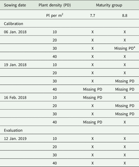
a Missing PD means that the intended plant density was not reached, therefore results were discarded.
Crop management was done according to the farm schedule, including seed treatment with insecticide and fungicide, followed by biological inoculant containing strains of Bradyrhizobium: SEMIA 5019 (B. elkanii) and SEMIA 5079 (B. japonicum) at an amount of 0.03 litres per ha. The soil fertilization was incorporated during sowing using 90 kg/ha of monoammonium phosphate (NPK: 12-61-0). Copper, cobalt and molybdenum were supplemented by foliar application. Weeds were controlled after sowing using glyphosate; pests were controlled by monitoring their presence every 5 days and diseases were controlled preventively, considering the action time of different chemical products; where these controls were aimed to avoid the presence of limiting factors.
Soil data collection
Soil chemical and physical attributes were sampled before sowing the field experiment at layers of 0–10, 10–20, 20–30, 30–50 and 50–70 cm depths. Four undisturbed samples were collected at the field using the volumetric ring to quantify soil water content at the soil saturation (SAT), at the drained upper limit (DUL), at the lower limit (LL) of plant extractable soil water, soil bulk density (BD) and hydraulic conductivity at saturation (KSAT) (Table 2), and three disturbed subsamples to quantify chemical and texture soil properties (Table 2). The DUL and LL points were quantified using the pressure plate method, respectively, at 10 and 1500 kPa. The initial soil water content was set at 50% of the difference between DUL and LL with the simulation initiated 30 days prior to the sowing date in the crop model.
Table 2. Soil layer characteristics measured prior to planting in the field experiment in Paragominas, PA

OM, organic matter; Presin, phosphorus extracted by ion exchange resins; CEC, cation-exchange capacity; V, base-cation saturation ratio; BD, soil bulk density; KSAT, hydraulic conductivity at saturation; SAT, soil water content at soil saturation; DUL, soil water content at drained upper limit; LL, lower limit of plant extractable soil water. The layer 70–300 cm was obtained extrapolating the last measured layer (50–70 cm). SRGF, soil root growth factor, obtained from Battisti et al. (Reference Battisti, Sentelhas and Boote2017).
Weather data collection
Daily weather data were obtained from an automatic weather station located at the experimental field, including maximum and minimum air temperature, total daily solar radiation and rainfall (Fig. 2). The mean (min–max) air temperatures were 26.4°C (18.9–38.8) and 27.0°C (19.8–37.3) respectively, for 2017/18 and 2018/19 growing seasons. The accumulated rainfalls were 1749 and 1928 mm from December to June, respectively, for 2017/18 and 2018/19 growing seasons. Total daily solar radiation had an average (min–max) of 18.2 (8.4–25.0) and 19.2 (6.5–28.6) MJ/m2/day, respectively, for 2017/18 and 2018/19 growing seasons. The climatology for the field experiment site (Paragominas) is shown in Fig. S1 of the Supplementary material.

Fig. 2. (Colour online) Maximum and minimum air temperature (a), total daily solar radiation (b and c) and rainfall (b and c) for field experiment conducted during 2017/18 (a and b) and 2018/19 (a and c) growing seasons. In (a), the arrow indicates the sowing date for soybean and in (b) and (c), the continuous line is total daily solar radiation and bar graph is rainfall.
Measurements
The phenological stages were monitored weekly, recording the date when at least 50% of plot plants achieved the phenological characteristics described by Boote et al. (Reference Boote, Jones, Batchelor, Nafziger and Myers2003). The phenological stages were sowing, emergence (VE, cotyledons above soil surface), first flower (R1, when one open flower appeared on any node on the main stem), first seed (R5, when 3 mm seeds appeared on any node on the main stem) and beginning maturity (R7, when one pod with mature colour appeared on any node on the main stem). Total above-ground biomass, stem, leaf, pod, grain, LAI and leaf number were measured from three to six times during the growing season by sampling 1 linear metre of a row (0.5 m2) from four replications. The samples occurred around 15, 30, 60, 75 and 90 days after sowing and at harvest for most of the treatments. Maturity group 7.7 did not have samples at 90 days after sowing, while for sowing dates on 16 Feb. 2018 and 12 Jan. 2019, the samples were done only at 40 and 75 days after sowing and at harvest.
The dry biomass was obtained after partitioning the plant in stem, leaf, pod and grain, drying at 70°C until constant weight. The LAI was determined by sampling leaves and scanning the whole leaf area with the LI-COR LI-3100C. The specific leaf area was calculated by dividing leaf area (cm2) by leaf biomass (g). Two central 1-m rows were harvested for final yield converted to dry mass, drying at 70°C until constant weight, and yield components (grain yield, number of pods, number of grains per pod and weight per grain). The harvest index was calculated by dividing grain yield by total aboveground biomass.
Crop model
Description of plant density response
The DSSAT CSM-CROPGRO-Soybean model v 4.7.0 (Hoogenboom et al., Reference Hoogenboom, Porter, Shelia, Boote, Singh, White, Hunt, Ogoshi, Lizaso, Koo, Asseng, Singels, Moreno and Jones2017) is widely used in Brazil for management evaluation, for example, for tropical conditions (Banterng et al., Reference Banterng, Hoogenboom, Patanothai, Singh, Wani, Pathak, Tongpoon-pol, Atichart, Srihaban, Buranaviriyakul, Jintrawet and Nguyen2009), climate response (Silva et al., Reference Silva, Pereira, Gonçalves, Bordignon and Marin2017; Battisti and Sentelhas, Reference Battisti and Sentelhas2019; Lima et al., Reference Lima, Oliveira, Sampaio, William and Souza2019) and irrigation (Battisti et al., Reference Battisti, Casaroli, Paixão, Alves Júnior, Evangelista, Mesquita, Mirschel, Terleev and Wenkel2020b). The response to plant density is influenced by the LAI which affects crop evapotranspiration and photosynthesis rates during the life cycle. Leaf area growth depends on canopy photosynthesis, partitioning of biomass to leaf and the specific leaf area (response to temperature, light and water deficit) (Boote and Pickering, Reference Boote and Pickering1994; Boote et al., Reference Boote, Jones, Hoogenboom, Pickering, Peart and Curry1998). The model simulates leaf senescence as a function of water deficit and nitrogen mobilization, as well as under high LAI because lower leaves receive low solar radiation. Plant density can indirectly affect water available to the crop through root density, as daily assimilate is partitioned to root mass and root length density leading to change in how the soil is explored and the availability of water to the crop (Boote et al., Reference Boote, Jones, Hoogenboom, Pickering, Peart and Curry1998). The root distribution with the soil profile depth is defined by the soil root growth factor (SRGF) (Table 2), and the same root profile shape was used for all plant densities in our study. The SRGF was obtained from Battisti et al. (Reference Battisti, Sentelhas and Boote2017).
Calibration and evaluation
The initial set of cultivar parameters for calibration was the generic cultivar parameters for maturity groups 7.0 and 8.0 from ecotype and cultivar file in the DSSAT-CROPGRO-Soybean for MG 7.7 and MG 8.8, respectively. The first step involved calibration of phenological coefficients such as first flower appearance (EM-FL), first pod (FL-SH) (adjusted to fit the onset of pod growth), first seed (FL-SD) and beginning maturity (SD-PM) (Hunt and Boote, Reference Hunt, Boote, Tsuji, Hoogenboom and Thornton1998), in combination with critical short day length (CSDL) and slope of the relative response of development to photoperiod (PPSEN). Adjustments using observations were done to reduce bias and the root mean square error (RMSE) (Wallach et al., Reference Wallach, Makowski and Jones2006), comparing measured and simulated values using scatter plots.
After phenology calibration, growth parameters were calibrated in the second step. These included the maximum leaf photosynthesis rate (LFMAX), defined at 30°C, 350 vpm of CO2 and high light; specific leaf area of cultivar under standard growth conditions (SLAVR); maximum size of full leaf (three leaflets) (SIZLF); time between first flower (R1) and end of leaf expansion (FL-LF); maximum weight per seed (WTPSD); seed filling duration for pod cohort at standard growth conditions (SFDUR); average seed number per pod under standard growing conditions (SDPDV); time required for cultivar to reach final pod load under optimal conditions (PODUR) and threshing percentage between grain and pod (THRSH).
Growth parameters were adjusted simultaneously using generalized likelihood uncertainty analysis (GLUE) (Makowski et al., Reference Makowski, Wallach and Tremblay2002; Jones et al., Reference Jones, Jianqiang, Boote, Wilkens, Porter, Hu, Ahuja and Ma2011) available within DSSAT to adjust LFMAX, SLAVR and SIZLF. The target of GLUE was only the final yield values. Therefore, subsequent manual calibration was done to improve the model performance against time-series growth analysis using scatter plots for yield, LAI and biomass partitioning, including bias and RMSE (Wallach et al., Reference Wallach, Makowski and Jones2006). The GLUE was set to run 15 000 simulations, following the recommendation of Jones et al. (Reference Jones, Jianqiang, Boote, Wilkens, Porter, Hu, Ahuja and Ma2011). After the optimization with GLUE and the manual calibration, parameters were checked to verify their consistency with other calibrations and maturity group characteristics in the model database. After calibration, the crop model was evaluated with independent data measured in the 2019 growing season (Table 2).
Model application over multiple weather seasons at six sites
Crop management was simulated using DSSAT's Seasonal Analysis software considering sowing dates, plant densities and maturity groups for six sites in northern Brazil. The sites were: Paragominas, Santarém, Santana do Araguaia, Anapurus, Balsas and Porto Nacional (Fig. 1). The daily weather data for 33 growing seasons were obtained from 01 Jan. 1980 to 31 Dec. 2013 (Xavier et al., Reference Xavier, King and Scanlon2015). The climatology for these sites can be found in Fig. S1 of the Supplementary material. The simulated crop management included four plant densities of 10, 20, 30 and 40 pl per m2; two maturity groups (7.7 and 8.8); and sowing dates every 10 days during the sowing windows for each region (Table 3), defined based on agroclimatic zoning risk (MAPA, 2020). The soil type and texture by site were obtained from RADAM (1974) (Table 3), while the soil water characteristics were obtained from Battisti and Sentelhas (Reference Battisti and Sentelhas2019) (Supplementary material, Table S1). The Seasonal Analysis was initiated 3 months prior to each sowing date, assuming initial soil water content at 50% of the difference between DUL and LL, with initial conditions reinitiated every growing season.
Table 3. Sites, geographic location, sowing window dates and soil type considered in the seasonal analyses for soybean management in the north Brazil

a Lat is the latitude.
b Long is the longitude.
c Elev is the elevation (m above sea level).
d Sowing was done every 10 days.
e Soil parameters are shown in Table S1 of the Supplementary material.
Results
Crop model performance compared to experimental data
The parameters calibrated can be found in Table 4 for MG 7.7 and 8.8. In the calibration process, the first step was to adjust parameters of CSDL and PPSEN to improve the prediction of first flower occurrence, followed by calibrating EM-FL, FL-SH, FL-SD and SD-PM. Then FL-LF, SLAVR and SIZELF were modified to improve LAI simulation, where it was necessary to modify parameters to improve LAI mainly for the lower plant density. FL-LF was increased for MG 7.7 due to its indeterminate flowering habit (start flowering early and indeterminate leaf area growth), while FL-LF for MG 8.8 was not changed from the generic default determine cultivar parameters because of its determinate growth habit. LFMAX was adjusted to increase biomass production, as this parameter increases both LAI and biomass. The default LFMAX value of 1.03 was increased to 1.20 and 1.175 μmol/m2/s, respectively, for MG 7.7 and 8.8. The final changes involved parameters related to pod and grain growth duration, to improve yield simulation (Table 4).
Table 4. Calibrated soybean cultivar parameters for the MG 7.7 and 8.8 in the CSM-CROPGRO-Soybean crop model

a Traits are described in Boote et al. (Reference Boote, Jones, Batchelor, Nafziger and Myers2003).
b V1-JU is in the ecotype file.
Phenology
For calibration, the model had a bias lower than 2 days for emergence, first flower, first seed and beginning maturity for MG 7.7 and 8.8 (Table 5), with a strong agreement between measured and simulated (Figs 3(a) and (b)). The evaluation was in agreement across crop stages for MG 7.7, with bias less than 1.3 days (Table 5) and strong agreement between measured and simulated (Fig. 3(a)). However, MG 8.8 showed a longer time to the occurrence of beginning maturity (bias = 7 days; Table 5); while anthesis occurred 4 days early in the crop model simulation (Table 5). There were no observed or simulated effects of plant density on crop phenology.

Fig. 3. Relationship between measured and simulated soybean crop stages (emergence, anthesis, first seed and maturity) for calibration and evaluation for maturity group 7.7 (a) and 8.8 (b). Absolute values and bias for calibration and evaluation steps can be found in Table 5.
Table 5. Measured (M), simulated (S), bias, RMSE and RRMSE (%) for crop end -season variables simulated by crop model in the calibration and evaluation steps for maturity groups (MG) 7.7 and 8.8

Time-series of leaf area index and biomass
LAI was simulated well across plant densities and sowing dates for MG 7.7 for both model calibration and evaluation processes (Fig. 4). For calibration, the RMSE was lower than 1.23 (relative RMSE (RRMSE) <33%; bias <1.08) (Supplementary material, Table S2). The later sowing dates (19 Jan. and 16 Feb.) showed a higher observed LAI than simulated, being higher during the middle to end of the cycle for 19 Jan. sowing (Fig. 4(b)), and a more rapid reduction for 16 Feb. (Fig. 4(c)). This performance was similar during evaluation for the sowing on 12 Jan. for four plant densities, with the field experiment having higher LAI late in the cycle when compared with simulated (Fig. 4(d)), although the crop model simulated higher main stem leaf (node) number during the evaluation (bias = 0.71) (Table 5).

Fig. 4. (Colour online) Measured (symbols) and simulated (line) LAI over time for calibration (a, b, c, e, f and g) and evaluation (d and h) for MG 7.7 (a, b, c and d) and MG 8.8 (e, f, g and h) at four plant densities. Mean measured and simulated values, bias, RMSE and RRMSE can be found in Table S2 of the Supplementary material.
The simulated and observed LAI were similar during the growing cycle for MG 8.8. A limitation was that the model overpredicted LAI for high plant density, as can be observed for 40 pl per m2 for sowing date on 06 Jan. (Fig. 4(e)) and 16 Feb. (Fig. 4(g)), where RRMSE was 28 and 19%, respectively (Supplementary material, Table S2). Simulated LAI was higher than observed for 10 pl per m2, where RRMSE were between 5 and 13% (Supplementary material, Table S2). For the model evaluation, the RRMSE increased with higher plant densities. RRMSE was 5% for 10 pl per m2, while it reached 32% at 40 pl per m2 (Supplementary material, Table S2).
The model response to plant density was well predicted for biomass and the individual components of biomass across crop cycle (pod, leaf and stem). The fractional partitioning between pod, leaf and stem for MG 7.7 was not affected by plant densities (true of the data as well as the model) (Figs 5(a–d)). For model calibration, the aboveground dry biomass for MG 7.7 had RMSE lower than 975 kg/ha (RRMSE <26%) (Supplementary material, Table S3) for time-series data, while for end-of-season, including all plant density, the overall RMSE was 489 kg/ha (RRMSE = 11.4%) (Table 5). The results from model evaluation revealed that RMSE for aboveground dry biomass increased to 1220 kg/ha, but with RRMSE of 21% for time-series data, while overall performance at end-of-season showed RMSE of 268 kg/ha (RRMSE = 4.6%) (Table 5). The bias for leaf and pod dry mass were similar during calibration and evaluation, being between −395 and −17 kg/ha for leaf (Supplementary material, Table S4), and between – 460 and 622 kg/ha for pod (Supplementary material, Table S5), showing agreement across crop cycle (Fig. 5). The LAI and leaf dry biomass resulted in a good simulation of specific leaf area for most of the plant densities (RRMSE between 2 and 40%), but with high RRMSE for low plant densities and early planting dates (Supplementary material, Table S7).

Fig. 5. (Colour online) Measured (symbols) and simulated (line) soybean above-ground biomass and partition to leaf, stem and pod over time for 10 pl per m2 (a, c, e and g) and 40 pl per m2 (b, d, f and h) sown on 06 Jan. 2018 (a, b, e and f) and 12 Jan. 2019 (c, d, g and h) for MG 7.7 (a, b, c and d) and 8.8 (e, f, g and h). Mean measured and simulated values, bias, RMSE and RRMSE can be found in Tables S3, S4, S5, S6 and S7 of the Supplementary material, respectively, for aboveground, leaf, pod and stem dry biomass.
The aboveground dry biomass was overpredicted by the model in the last date of measurement for MG 8.8 in the calibration and evaluation (Figs 5(e–h)). As expected, the RMSE aboveground dry biomass was larger for 40 than for 10 pl per m2 (increasing from 499 to 652 kg/ha in calibration and from 798 to 1206 kg/ha in evaluation) (Supplementary material, Table S3). The model simulated well the values and the dynamics of aboveground dry biomass (Figs 5(e–h)), with RRMSE ranged from 7 and 16% for calibration, and 21 to 28% for evaluation (Supplementary material, Table S3). The leaf dry mass had low RRMSE during calibration (between 13 and 22%) (Supplementary material, Table S4) than during evaluation, when RRMSE increased from 10 to 33% with plant densities, respectively, from 10 to 40 pl per m2 (Supplementary material, Table S4); although specific leaf area had a similar RRMSE, from 7 to 27% during calibration, and from 11 to 21 during evaluation (Supplementary material, Table S7).
Grain yield
Grain yield had an RMSE and RRMSE, respectively, of 401 kg/ha and 12% for calibration, and 119 kg/ha and 3% for evaluation for MG 7.7 (Fig. 6(a)). The biases were 88 and 21 kg/ha, respectively, for calibration and evaluation (Table 5). MG 8.8 had similar performance for calibration to MG 7.7, resulting in a RMSE and RRMSE, respectively, of 384 kg/ha and 10% (Fig. 6(b)), with a bias of −24 kg/ha (Table 5). However, RRMSE was larger for evaluation of MG 8.8, with 32% (RMSE = 1035 kg/ha) and a bias of 986 kg/ha (Fig. 6(b)). In this case, the model showed a yield response higher than field experiments across plant densities.

Fig. 6. Relation between simulated and measured soybean grain yield for calibration and evaluation for maturity group 7.7 (a) and 8.8 (b). RMSE is the root mean square error and RRMSE is the relative root mean square error.
Seasonal analysis application: sowing dates × plant density × cultivars
Seasonal analysis over 33 seasons showed that higher plant density (40 pl per m2) resulted in higher yield than lower plant density for all locations, sowing dates and maturity group (Fig. 7). However, the yield increase was greater when plant density was increased from 10 to 20 pl per m2, followed by 20 to 30 pl per m2 and 30 to 40 pl per m2. The higher yield difference between plant density occurred for the sowing date on 21 Feb. and MG 8.8 in Santarém. Under this condition, median yields were 2658, 3197, 3442 and 3583 kg/ha (Fig. 7(f)), respectively, for 10, 20, 30 and 40 pl per m2. The yield increase was 20, 8 and 4%, respectively, from 10 to 20, 20 to 30 and 30 to 40 pl per m2. Porto Nacional had the lower response with plant density increase for MG 8.8, from 1.2 to 7.3%, with a median yield across sowing dates of 2991, 3211, 3293 and 3332 kg/ha, respectively, for 10, 20, 30 and 40 pl per m2 (Fig. 7(j)).

Fig. 7. (Colour online) Soybean grain yield simulated as a function of plant density (10 to 40 pl per m2), sowing dates and maturity groups 7.7 (a, c, e, g, i and k) and 8.8 (b, d, f, h, j and l) across 33 growing seasons in Anapurus (a and b), Paragominas (c and d), Santarém (e and f), Balsas (g and h), Porto Nacional (i and j) and Santana do Araguaia (k and l). In the box-plot, the central line is the medium, the lower and upper hinges correspond to the first and third quartiles (the 25th and 75th percentiles), the upper and lower whisker extends from the hinge to the largest and smallest value, respectively, than 1.5 × IQR from the hinge (where IQR is the inter-quartile range, or distance between the first and third quartiles), and data beyond the end of the whiskers are called ‘outlying’ points and are plotted individually. The red dashed line is the mean value across plant density and sowing date.
The yield across sowing dates had a similar response for MG 7.7 and 8.8 in Anapurus (Figs 7(a) and (b)), Paragominas (Figs 7(c) and (d)) and Santarém (Figs 7(e) and (f)). The greater inter-annual yield variability occurred at the beginning of sowing window (01 Dec. and 11 Dec.), due to limiting weather conditions that can occur at the beginning of the sowing window. The delay of the sowing date increased the yield difference between plant densities in these sites. For example, the median yield for MG 7.7 with 40 pl per m2 density was 635 kg/ha (25%) greater than that with 10 pl per m2 for the 01 Dec. sowing date, and this yield difference between plant densities was 820 kg/ha (38%) for the 21 Feb. sowing date. For these three sites, the median yield typically reduced on delaying the sowing date, and the yield reduction with delayed sowing was larger for the lowest planting density than for the highest planting density. For example, the difference yield for MG 7.7 with 10 pl per m2 sowing on 01 Dec. and 21 Feb. was 415 kg/ha, while this difference was 230 kg/ha for 40 pl per m2.
The sowing dates resulted in two patterns of yield when considered MG 7.7 (Fig. 7(g)) and MG 8.8 (Fig. 7(h)) in Balsas. The two maturity groups showed very similar potential yield in the region, with, respectively, a mean yield of 3408 and 3335 kg/ha. MG 7.7 increased median yield, averaged across planting densities, from 3448 kg/ha on 01 Oct. to 3895 kg/ha on 11 Nov., reducing after that date until 21 Jan. In this scenario, the sowing date affects the yield difference between plant density, where early sowing date (01 Oct.) showed a mean difference between 10 and 40 pl per m2 of 453 kg/ha, while late sowing (21 Jan.) reached a difference of 662 kg/ha. However, MG 8.8 increased median yield, averaged across planting densities, from 3133 kg/ha on 01 Oct. to 3772 kg/ha on 21 Dec., reducing after data until 21 Jan.
Porto Nacional (Figs 7(i) and (j)) and Santana do Araguaia (Figs 7(k) and (l)) had similar yield levels and patterns across sowing dates, maturity groups and plant densities. MG 7.7 had a similar yield from 01 Oct. to 21 Nov., with a reduction until 21 Dec. for plant density of 20, 30 and 40 pl per m2. However, plant density of 10 pl per m2 showed a lower yield at the start and end of the sowing window, with the best sowing date occurring on 11 Nov., with a median yield of 3637 and 3591 kg/ha, respectively, for Porto Nacional (Fig. 7(i)) and Santana do Araguaia (Fig. 7(k)). The delay of sowing from 01 Oct. to 21 Dec. increased yield for MG 8.8, showing lower potential and yield difference between plant densities than MG 7.7 (Figs 7(j) and (l)).
Discussion
CSM-CROPGRO-Soybean demonstrated good performance for both MG 7.7 and 8.8 in response to plant densities and sowing dates in this short photoperiod low latitude environment. The performance of the model as described by statistical indices are similar to prior studies in Brazil for the north (Lima et al., Reference Lima, Oliveira, Sampaio, William and Souza2019), midwestern (Teixeira et al., Reference Teixeira, Battisti, Sentelhas, de Moraes and de Oliveira Junior2019) and southern (Battisti et al., Reference Battisti, Sentelhas and Boote2017) regions. Furthermore, a characteristic not accounted for by Grimm et al. (Reference Grimm, Jones, Boote and Hesketh1993) in the default parameters is the presence of long juvenile phase introduced into soybean germplasm adapted to low latitude (Destro et al., Reference Destro, Afonso, Kiihl, Alves and Almeida2001; Carpentieri-Pípolo et al., Reference Carpentieri-Pípolo, de Almeida and de Kiihl2002; Sinclair et al., Reference Sinclair, Neumaier, Farias and Nepomuceno2005; Alliprandini et al., Reference Alliprandini, Abatti, Bertagnolli, Cavassim, Gabe, Kurek, Marsumoto, Oliveira, Pitol, Prado and Steckling2009; Liu et al., Reference Liu, Wu, Ren, Qi, Li, Cao, Zhang, Zhang, Cai and Gai2017). A value of 6 thermal days was added to the ecotype parameter time required from first true leaf to end of the juvenile phase (V1-JU) (Table 4), which led to minimal effect of short photoperiod of this region on the time for first flower occurrence. However, this did not work as intended, therefore the effect of the juvenile trait was created by using a longer EM-FL parameter duration than the generic cultivar parameters presented by Boote et al. (Reference Boote, Jones, Batchelor, Nafziger and Myers2003).
The model had poorer phenology performance during the evaluation (2019 growing season) for MG 8.8. The crop model followed the same pattern for evaluation as for calibration, while the observed crop in the evaluation had a longer vegetative period (4-day delay of the first flower) and a shorter time from first flowering to beginning maturity (7 days earlier to beginning maturity). We hypothesize that this occurred because of an effect of water excess in the field associated with high cultivar sensitivity (Bajgain et al., Reference Bajgain, Kawasaki, Akamatsu, Tanaka, Kawamura, Katsura and Shiraiwa2015; Pasley et al., Reference Pasley, Huber, Castellano and Archontoulis2020). The crop model simulated a penalization for water excess lower than 1% (data not shown). The potential water excess can be verified based on a high frequency of rainy days during the growing seasons (Figs 2(b) and (c)), where the accumulated rainfalls were 1749 and 1928 mm from December to June, respectively, for 2017/18 and 2018/19 growing seasons.
CROPGRO-Soybean does simulate canopy height and width and does account for row spacing (Boote et al., Reference Boote, Jones, Hoogenboom, Pickering, Peart and Curry1998) an approach required for its hedgerow light interception. Plant structure changes considerably across plant density due to soybean plasticity (Supplementary material, Fig. S2) (Carpenter et al., Reference Carpenter and Board1997; Balbinot Junior et al., Reference Balbinot Junior, de Oliveira, Zucareli, Ferreira, Werner and Silva2018; Ferreira et al., Reference Ferreira, Zucareli, Werner, Fonseca and Balbinot Junior2020). The plasticity increases branch number under low plant density in response to solar radiation interception, light quality and plant competition (Board, Reference Board2000; Nakano et al., Reference Nakano, Purcell, Homma and Shiraiwa2019). The leaf senescence was smaller in the field than in the crop model from the middle to the end of the cycle under low plant density (10 pl per m2). This may be associated with a less self-shading effect and a high number of branches, and high light may slow nitrogen mobilization from leaves, thus reducing leaf senescence (Boote and Pickering, Reference Boote and Pickering1994).
The interaction between maturity group, sowing dates and plant densities affected LAI dynamics and, consequently, potential yield. For example, MG 7.7 had LAI reaching value 3 later in the cycle (80 days after sowing) for 10 pl per m2 (Figs 4(a), (b) and (d)), while plant densities above 20 pl per m2 reached the LAI 3 value in less than 50 days after sowing.
A higher plant density typically increases aboveground biomass and LAI, but yield increase is conditioned by the cultivar adaptation to a given environment (Ball et al., Reference Ball, Purcell and Vories2000; Board, Reference Board2000; Corassa et al., Reference Corassa, Amado, Strieder, Schwalbert, Pires, Carter and Ciampitti2018; Carciochi et al., Reference Carciochi, Schwalbert, Andrade, Corassa, Carter, Gaspar, Schmidt and Ciampitti2019). The crop model simulated well the yield, biomass and LAI for most cases across plant density and sowing dates. However, for MG 8.8 (determinate growth) sowing on 12 Jan. 2019 (Fig. 5(h)), the higher plant density did not result in an increase of yield at the field, while the crop model did increase yield in response to high plant density.
Seasonal analysis showed a higher soybean grain yield for a plant density of 40 pl per m2, as expected (Fig. 7). However, a considerable yield increase occurred from 10 to 20 pl per m2. This indicates that a minimum of plant density over 20 pl per m2 is required for these sites (Fig. 7), ensuring soybean yield stability across sowing dates. The soybean plasticity across plant density is associated with adjustment in branch number, pod and seed number by area (Supplementary material, Fig. S2). The resultant effects include increased biomass partitioned to branches, the net photosynthesis, the efficiency of solar radiation interception by leaf area during the vegetative phase and the leaf expansion during reproductive phase (Carpenter and Board, Reference Carpenter and Board1997; Ball et al., Reference Ball, Purcell and Vories2000; Board, Reference Board2000; Balbinot Junior et al., Reference Balbinot Junior, de Oliveira, Zucareli, Ferreira, Werner and Silva2018).
Plant density higher than 20 pl per m2 showed higher yield, however, it is essential to consider cultivars resistance to lodging and the potential pressure of diseases in the region. These are conditions that can lead to yield losses when higher plant densities are used, and lodging and pests are not accounted for yield penalization by the crop model (Teixeira et al., Reference Teixeira, Battisti, Sentelhas, de Moraes and de Oliveira Junior2019). For example, Paragominas has a higher rainfall amount during the reproductive period when sowing occurs in January (Supplementary material, Fig. S1). High rainfall amount increases soybean rust pressure due to leaf wetness (Del Ponte et al., Reference Del Ponte, Godoy, Li and Yang2006), where a plant density between 20 and 30 pl per m2 has a preference to reach high potential yield and reduce diseases risk by lower leaf area (lower leaf wetness and more efficiency of application of chemical control).
The maturity group and sowing dates affected the interaction between local weather and plant density over yield due to cycle duration and the time to achieve the optimum LAI for maximum light interception (Purcell et al., Reference Purcell, Ball, Reaper and Voires2002; Lee et al., Reference Lee, Egli and TeKrony2008; Zdziarski et al., Reference Zdziarski, Todeschini, Milioli, Woyann, Madureira, Stoco and Benin2018). For the sites of low latitude, between 2° and 4° south, MG 8.8 had preference over MG 7.7 due to the higher average and stability yield across sowing window, while for sites below latitude 9° south, MG 7.7 had the preference of sowing. On the contrary, Balsas (latitude 8° south) had a similar average yield across sowing window for MG 7.7 and MG 8.8, but with the higher yield occurring for sowing dates, respectively, in November and December.
The maturity groups and sowing date patterns by location occurred due to cycle duration and potential yield associated with climate (Battisti and Sentelhas, Reference Battisti and Sentelhas2019). The cycle duration defines the capacity of the crop to intercept solar radiation and, consequently, the potential yield (Van Roekel et al., Reference Van Roekel, Purcell and Salmerón2015). The longer cycle (MG 8.8) was a better strategy for low latitude, where water deficit is lower and longer cycle results in higher potential yield (Battisti and Sentelhas, Reference Battisti and Sentelhas2019). The sites of higher latitude showed a preference for MG 7.7, mainly for early sowing dates. On the contrary, MG 8.8 had a higher yield for late sowing dates in Balsas, and a lower yield difference between MG 8.8 and MG 7.7 with early sowing dates in Porto Nacional and Santana do Araguaia. This occurred due to the photoperiod reduction in late sowing dates accelerates the crop cycle of MG 7.7, resulting in less time for the crop to increase leaf area in low plant densities (Tagliapietra et al., Reference Tagliapietra, Streck, da Rocha, Richter, da Silva, Cera and Junior Zanon2018).
Conclusion
CSM-CROPGRO-Soybean was able to simulate crop development and growth across maturity groups, sowing dates and plant densities in the short-day low latitude environment. Multi-year seasonal analysis indicated that plant density of 40 pl per m2 leads to higher yield in all sites, sowing dates and maturity groups simulated in the crop model. However, high plant density can lead to yield losses by plant lodging and increase disease pressure by higher leaf area, increasing leaf wetness and reducing the efficiency of application of chemical control. Lodging and diseases are factors that crop models are not accounted for in yield simulation. Overall, the 20 pl per m2 is a minimum plant density required for soybean production in this region, due to the higher yield increase that occurred when plant density was increased from 10 to 20 pl per m2, leading to high yield gain and relive to lower seed costs. Further to plant density, the planning of maturity groups and sowing dates by sites showed to be important factors by the different response patterns, which can help to improve soybean yield.
Supplementary material
The supplementary material for this article can be found at https://doi.org/10.1017/S0021859621000204.
Acknowledgements
The authors would like to thank the Juparanã Agrícola farm for field support; the Universidade Federal de Santa Catarina for the post-doc position for the first author in the Postgraduate Program in Agroecosystems, especially for the contribution from Prof. Dr S. L. Schlindwein.
Financial support
Support for the second author from the National Council for Scientific and Technological Development (CNPq) through Financial Support to Research (Process No. 405740/2018-2) is gratefully acknowledged.
Conflict of interest
None.


