


1. Introduction
Suspensions of solid particles are ubiquitous in environmental (landslides), industrial (waste slurries) and biological flows (blood), and their study has continued to yield new discoveries (Jeffrey & Acrivos Reference Jeffrey and Acrivos1976; Stickel & Powell Reference Stickel and Powell2005). The vast majority of previous efforts were dedicated to Newtonian suspensions, while in many applications the suspending fluid is non-Newtonian (Chhabra Reference Chhabra2006). Viscoelasticity is a prominent non-Newtonian effect that alters the rheological and transport properties of the flow in complex and often unexpected ways, even in the absence of the particle phase. For instance, the addition of minute amounts of polymer additives to turbulent pipe flow renders the fluid viscoelastic, weakens the turbulence activity, and reduces the drag (Toms Reference Toms1948). In the absence of turbulence, however, the same practice can destabilize the flow in the transitional regime (Samanta et al. Reference Samanta, Dubief, Holzner, Schäfer, Morozov, Wagner and Hof2013; Lee & Zaki Reference Lee and Zaki2017) and can give rise to elastic turbulence in the absence of inertia (Groisman & Steinberg Reference Groisman and Steinberg2000). In this study, we computationally investigate the combined effects of viscoelasticity and concentrated particle suspension on the dynamics of turbulent channel flow. We begin with a brief account of the rheological properties of viscoelastic suspensions in the absence of turbulence, followed by a summary of the effects of fluid inertia and turbulence on particle-laden flows; the latter studies being mostly limited to Newtonian fluids.
1.1. Viscoelastic suspensions in inertialess flows
Early theoretical developments by Einstein for dilute Newtonian suspensions in the absence of inertia predict a relative increase in the so-called effective viscosity, or the bulk shear viscosity of the mixture, at a rate of  $\sim (5/2)\varphi$ where
  $\varphi$ is the bulk solid volume fraction (Happel & Brenner Reference Happel and Brenner2012). Einarsson, Yang & Shaqfeh (Reference Einarsson, Yang and Shaqfeh2018) reported a correction to the Einstein relation in the same limit of dilute suspension, but when the background fluid is viscoelastic. The shear dependent rheology of such suspensions, including for Boger fluids, exhibits shear-thickening (Zarraga, Hill & Leighton Reference Zarraga, Hill and Leighton2001; Scirocco, Vermant & Mewis Reference Scirocco, Vermant and Mewis2005). Two-dimensional numerical simulations confirmed this effect in disk suspensions in Oldroyd-B fluids (Hwang, Hulsen & Meijer Reference Hwang, Hulsen and Meijer2004). In a linear velocity field and in the limit of Weissenberg number
  $Wi \equiv \dot {\gamma } \lambda \ll 1$, where
  $\dot {\gamma }$ and
  $\lambda$ are the shear rate and the viscoelastic relaxation time, Koch & Subramanian (Reference Koch and Subramanian2006) theoretically explained that the contribution of particles to the bulk stress is two-fold: (i) polymer stresses modify the particle stresslet; (ii) velocity and pressure disturbances in the vicinity of the particles alter the polymer stress in the fluid. Recently, Yang & Shaqfeh (Reference Yang and Shaqfeh2018a) extended this analysis to moderate and high-Weissenberg numbers by boundary-fitted numerical simulations of a single sphere. Reportedly, the regions that contribute most to particle-induced fluid stresses are close to the sphere surface where streamlines form closed trajectories. In another effort, Yang & Shaqfeh (Reference Yang and Shaqfeh2018b) investigated suspensions at finite solid volume fractions (
 $\varphi < 10\,\%$), and concluded that particle–particle interactions have a negligible influence on the bulk rheology of the flow.
At non-dilute concentrations ( $10\,\% <\varphi < 40\,\%$), previous studies reported a nonlinear relation between the effective viscosity and the solid volume fraction in both Newtonian and viscoelastic fluids (Denn & Morris Reference Denn and Morris2014; Dai & Tanner Reference Dai and Tanner2017). For the latter, studies of filled molten polymers highlight a complex rheology which primarily depends on the diffusion time scale of fillers (Brownian or non-Brownian particles), but also their shape, concentration, and nature of the carrier fluid (see Rueda et al. (Reference Rueda, Auscher, Fulchiron, Perie, Martin, Sonntag and Cassagnau2017), for a review). For other non-Newtonian effects, such as variable-viscosity and yield-stress fluids, we refer the reader to the review of Tanner (Reference Tanner2019).
1.2. Inertial effects and turbulence
In the presence of fluid inertia, the effective viscosity of suspensions increases. In the laminar regime, this observation is attributed to multiple effects, including the Reynolds stresses induced by particle fluctuations (Kulkarni & Morris Reference Kulkarni and Morris2008), particle and fluid phase acceleration (Rahmani, Hammouti & Wachs Reference Rahmani, Hammouti and Wachs2018) and anisotropy in microstructure leading to higher effective solid volume fractions (Picano et al. Reference Picano, Breugem, Mitra and Brandt2013). Since viscoelasticity influences both the hydrodynamic forces experienced by particles (Becker et al. Reference Becker, McKinley, Rasmussen and Hassager1994) and the local microstructure (D'Avino & Maffettone Reference D'Avino and Maffettone2015), it is interesting to consider whether and how the increase in effective viscosity is influenced by viscoelastic effects in the carrier fluid.
Beyond a critical Reynolds number, transition to turbulence takes place and the shear stress increases dramatically – a phenomenon that is modulated by both finite-size particles (Matas, Morris & Guazzelli Reference Matas, Morris and Guazzelli2003) and viscoelasticity (Draad, Kuiken & Nieuwstadt Reference Draad, Kuiken and Nieuwstadt1998; Lee & Zaki Reference Lee and Zaki2017). Dilute particle suspensions can promote instability and sustain a turbulent state at lower Reynolds numbers than a single-phase flow (Matas et al. Reference Matas, Morris and Guazzelli2003; Loisel et al. Reference Loisel, Abbas, Masbernat and Climent2013). Beyond the transitional regime, the literature on particle-turbulence interactions in a Newtonian fluid is extensive (cf. introduction by Agarwal, Brandt & Zaki (Reference Agarwal, Brandt and Zaki2014); Esteghamatian & Zaki (Reference Esteghamatian and Zaki2019), for a review). In brief, the effect of particles on Newtonian turbulence primarily depends on the solid volume fraction and the relative size of particles with respect to the Kolmogorov scale. In a concentrated suspension of finite-size spherical particles in wall-bounded turbulence, the Reynolds shear stress is attenuated. However, due to the addition of particle stresses the overall drag is increased (Shao, Wu & Yu Reference Shao, Wu and Yu2012; Picano, Breugem & Brandt Reference Picano, Breugem and Brandt2015). Hence, the propensity of particles to increase the drag grows with the solid volume fraction. In viscoelastic single-phase flows, linear theory has been developed to explain the new phenomenology that arises in the vorticity dynamics of wall-bounded flows, e.g. re-energization of streaks, reverse-Orr amplification, and non-local amplification of vorticity away from curved surfaces (Page & Zaki Reference Page and Zaki2014, Reference Page and Zaki2015, Reference Page and Zaki2016). A rigorous mathematical framework was also developed recently to derive perturbative expansion of the conformation tensor while maintaining the physical and geometrical consistency (Hameduddin, Gayme & Zaki Reference Hameduddin, Gayme and Zaki2019). A wealth of studies have been dedicated to the fully turbulent region (see review by White & Mungal (Reference White and Mungal2008)), and the mathematical theory has shed light on the appropriate mean polymer conformation tensor and measures of the disturbances relative to that mean (Hameduddin et al. Reference Hameduddin, Meneveau, Zaki and Gayme2018; Hameduddin & Zaki Reference Hameduddin and Zaki2019).
Very limited studies have been dedicated to the combined effects of finite-size particles, viscoelasticity and turbulence. For particles smaller than the Kolmogorov scale (in one-way coupling regime), De Lillo, Boffetta & Musacchio (Reference De Lillo, Boffetta and Musacchio2012) and Nowbahar et al. (Reference Nowbahar, Sardina, Picano and Brandt2013) investigated the influence of viscoelasticity on the particle clustering. In a weakly viscoelastic duct flow, experimental findings by Zade, Lundell & Brandt (Reference Zade, Lundell and Brandt2019) reported a less effective drag reduction in the particle-laden condition compared with the single-phase counterpart. For suspensions at dilute limits ( $\varphi =5\,\%$), while the particles significantly contribute to the turbulence suppression, Esteghamatian & Zaki (Reference Esteghamatian and Zaki2019) showed that they can also modify the cycles of low and high turbulence intensity which Xi & Graham (Reference Xi and Graham2010) termed ‘hibernating’ and ‘active’ turbulence. Extended periods of hibernating turbulence gives rise to the particles’ migration towards the channel centre, while the infrequent bursts of active turbulence redistributes the particles across the channel. Given the dual effect of particles in attenuating the Reynolds stresses while increasing the polymer stresses, the newly established momentum balance is expected to depend on the solid volume fraction. However, similar detailed studies of particle-laden viscoelastic flows at higher particle concentrations are absent from the literature – a matter that is addressed herein.
The present study reports on direct numerical simulations of particle-laden viscoelastic turbulent flows at 20 % solid volume fraction and over a wide range of viscoelasticity. The computations resolve the flow at the scale of particles, and polymer forces are obtained by solving an evolution equation for the polymer conformation tensors. The flow configuration, governing equations and computational set-up are described in § 2. Drag modulations, polymer and turbulence modification, and particle dynamics are analysed in § 3. Concluding remarks are provided in § 4.
2. Flow configuration and numerical approach
The computational domain is a plane channel, where  $x$,
$x$,  $y$ and
  $z$ correspond to the streamwise, wall-normal and spanwise directions (figure 1). The flow is maintained at a constant mass flux in the
  $x$ direction. The bulk velocity,
  $U_b$, and the channel half-height,
  $h$, are chosen as characteristic scales. The associated Reynolds and Weissenberg numbers are
  $Re \equiv hU_b/\nu$ and
  $Wi \equiv \lambda U_b/h$, where
  $\nu$ and
  $\lambda$ are the fluid total kinematic viscosity and viscoelastic relaxation time. When present, particles are spherical, their density matches that of the fluid
  $\rho$, and their diameter is denoted
  $d_p$. The bulk volume fraction is
  $\varphi \equiv N_p \mathcal {V}_p/\mathcal {V}_t$, where
  $N_p$,
  $\mathcal {V}_p$ and
  $\mathcal {V}_t$ are the total number of particles, the volume of a particle and the volume of the computational domain. The flow is periodic in the
  $x$ and
  $z$ directions, while a no-slip boundary condition is set at the bottom and top walls
  $y=\{0,2\}$, as well as at the surfaces of particles.

Figure 1. Schematic of the particle-laden flow configuration. Periodic boundary conditions are imposed in the  $x$ and
  $z$ directions, and no-slip conditions
  $\boldsymbol {u}_f = 0$ are enforced at
  $y=\{0,2\}$.
The non-dimensional governing equations for the fluid velocity  $\boldsymbol {u}_f$, the hydrodynamic pressure
  $p$, and the conformation tensor
  $\boldsymbol{\mathsf{c}}$ are
 \begin{gather} \boldsymbol{\nabla}\boldsymbol{\cdot}{\boldsymbol{u}_f} = 0, \end{gather}
 \begin{gather}\dfrac{\partial{\boldsymbol{u}_f}}{\partial{t}} + \boldsymbol{u}_f \boldsymbol{\cdot} \boldsymbol{\nabla}{\boldsymbol{u}_f}+\boldsymbol{\nabla}{p} - \dfrac{\beta}{Re} \nabla^2{\boldsymbol{u}_f} - \dfrac{1-\beta}{Re} \boldsymbol{\nabla}\boldsymbol{\cdot}{{\boldsymbol{\mathsf{T}}}} - \boldsymbol{F} = 0, \end{gather}
 \begin{gather}\dfrac{\partial{\boldsymbol{\mathsf{c}}}}{\partial{t}} +\boldsymbol{u}_f \boldsymbol{\cdot} \boldsymbol{\nabla}{\boldsymbol{\mathsf{c}}}- \boldsymbol{\mathsf{c}} \boldsymbol{\cdot} \boldsymbol{\nabla}{\boldsymbol{u}_f} - (\boldsymbol{\mathsf{c}} \boldsymbol{\cdot} \boldsymbol{\nabla}{\boldsymbol{u}}_f)^\textrm{T} - {\boldsymbol{\mathsf{T}}} = 0. \end{gather}
The solvent to total viscosity ratio is denoted  $\beta \equiv {\mu _s}/{\mu _s+\mu _p}$, where
  $\mu _s$ and
  $\mu _p$ denote the solvent and polymer contributions, and
  $\boldsymbol {F}$ represent a generic force field. Additionally, the viscoelastic stress tensor
  ${\boldsymbol{\mathsf{T}}}$ is expressed in terms of the conformation tensor with a FENE-P model,
 \begin{equation} {\boldsymbol{\mathsf{T}}} \equiv \dfrac{1}{Wi} \left(\dfrac{\boldsymbol{\mathsf{c}}}{\psi}-\dfrac{\boldsymbol{\mathsf{I}}}{a} \right), \quad \psi = 1 - \dfrac{\text{tr}(\boldsymbol{\mathsf{c}})}{L^2_{max}}, \quad a = 1- \dfrac{3}{L^2_{max}}, \end{equation}
where  $\boldsymbol{\mathsf{I}}$ and
  $L_{max}$ are the unit tensor and maximum extensibility of the polymer chains. The rigid-body motion of particles is governed by the Newton–Euler equations,
 \begin{gather} {\mathcal{V}_p} \dfrac{\boldsymbol{\text{d}}{\boldsymbol{u}_p}}{\text{d}{t}} = \oint_{\partial {\mathcal{V}_p}} \boldsymbol{\sigma}_f \boldsymbol{\cdot} \boldsymbol{n} \,\text{d} \mathcal{A} + \boldsymbol{F}_c, \end{gather}
 \begin{gather}\mathcal{I}_p \dfrac{\boldsymbol{\text{d}}{\boldsymbol{\omega}_{\boldsymbol{p}}}}{\text{d}{t}} = \oint_{\partial {\mathcal{V}_p}} \boldsymbol{r} \times \boldsymbol{\sigma}_f \boldsymbol{\cdot} \boldsymbol{n} \,\text{d} \mathcal{A}, \end{gather}
where  $\boldsymbol {u}_p$ and
  $\boldsymbol {\omega }_p$ are the particle translational and angular velocities. The hydrodynamic stress tensor comprising both Newtonian and viscoelastic contributions is denoted
  $\boldsymbol {\sigma }_f$, while
  ${\mathcal {V}_p} = {{\rm \pi} d_p^3}/{6}$ and
  ${\mathcal {I}_p}= {{\rm \pi} d_p^5}/{60}$ are the dimensionless volume and moment of inertia of a spherical particle. The particle–particle and particle–wall repulsive collision forces,
  $\boldsymbol {F}_c$, are adopted from Glowinski et al. (Reference Glowinski, Pan, Hesla, Joseph and Périaux2001), and are applied in the opposite direction to the outward unit vector
  $\boldsymbol {n}$ at the surface.
For a detailed description of the herein-adopted numerical algorithm for simulating particle-laden viscoelastic turbulence, the reader is referred to Esteghamatian & Zaki (Reference Esteghamatian and Zaki2019). For completeness, only the principal features of the algorithm are summarized here: the flow equations (2.1) and (2.2) are discretized using a control volume formulation and marched in time by a fractional step method (Rosenfeld, Kwak & Vinokur Reference Rosenfeld, Kwak and Vinokur1991). The diffusion terms are treated implicitly by a Crank–Nicolson scheme, while an explicit Adams–Bashforth scheme is adopted for advection. The conformation-tensor (2.3) are solved using a third-order accurate Runge–Kutta method, an explicit Adams–Bashforth discretization for advection and stretching terms and a semi-implicit approach for the polymer stress term in order to ensure finite extensibility of the polymers (Dubief et al. Reference Dubief, Terrapon, White, Shaqfeh, Moin and Lele2005; Lee & Zaki Reference Lee and Zaki2017). The advection term in (2.3) is evaluated with a second-order accurate spatial discretization as long as the conformation tensor remains positive definite; when its smallest eigenvalue approaches zero, the discretization is replaced by the one-sided difference which maximizes the minimum eigenvalue (see appendix B in Hameduddin et al. (Reference Hameduddin, Meneveau, Zaki and Gayme2018)). A sharp-interface immersed boundary force field (Nicolaou, Jung & Zaki Reference Nicolaou, Jung and Zaki2015) is employed to enforce a no-slip boundary condition at the surface of the particles ( $\boldsymbol {F} = \boldsymbol {F}_{\text {IB}}$ in (2.2)), and the conformation tensor is set to unity inside the solid domain. In addition, a short-range repulsive force equivalent to the one proposed by Glowinski et al. (Reference Glowinski, Pan, Hesla, Joseph and Périaux2001) is used to avoid particle–particle and particle–wall overlap.
Our numerical method has been previously validated in single-phase Newtonian (Lee et al. Reference Lee, Jung, Sung and Zaki2013) and viscoelastic turbulence (Lee & Zaki Reference Lee and Zaki2017), as well as in several fluid/particle configurations in both Newtonian and viscoelastic conditions (Esteghamatian & Zaki Reference Esteghamatian and Zaki2019). In the Appendix, we present an additional validation case to demonstrate the accuracy of our particle-laden viscoelastic solver in the simulation of lateral migration of a sphere in Newtonian and viscoelastic fluids.
Direct numerical simulations were performed for a Newtonian and five viscoelastic fluids, each without and with the particle phase. The physical and computational parameters of the simulations are provided in table 1. In the Newtonian single-phase configuration, the friction Reynolds number  $Re_\tau \equiv hu_\tau /\nu \approx 180$, where
  $u_\tau \equiv \sqrt {\langle \tau _{w} \rangle /\rho }$ denotes the friction velocity and
  $\langle \tau _{w} \rangle$ is the average wall shear stress. In particle-laden cases, the particle size in wall units
  $d_p\nu /u_\tau$ ranges from 18 to 21. A designation is introduced to identify each flow configuration: the letter
  $W$ is followed by the Weissenberg number
  $Wi$ and
  $P$ by the bulk solid volume fraction of the system
  $\varphi (\%)$.
Table 1. Physical and computational parameters of the simulations. Reynolds number  $Re \equiv hU_b/\nu$ and Weissenberg number
  $Wi \equiv \lambda U_b/h$ are based on the channel half-height
  $h$, the bulk velocity
  $U_b$, total kinematic viscosity
  $\nu$ and viscoelastic fluid relaxation time
  $\lambda$. The domain sizes are
  $L_{\{x,y,z\}}$ in the
  $\{x,y,z\}$ directions, and the numbers of grid cells are
  $N_{\{x,y,z\}}$. The noted line types and symbols are adopted in all figures unless otherwise stated.

The computational grid was uniform in the streamwise and spanwise directions. In the wall-normal direction, the grid spacing was also uniform in the particle-laden simulations and a hyperbolic tangent grid stretching was adopted in the single-phase simulations. In order to properly capture the flow field in the vicinity of the particles, the grid-cell size in those simulation was set to  $d_p/ {\rm \Delta} x=16$, commensurate with earlier studies (Goyal & Derksen Reference Goyal and Derksen2012; Costa et al. Reference Costa, Picano, Brandt and Breugem2018).
Randomly seeded particles naturally trigger the breakdown to turbulence in the Newtonian cases, while the single-phase Newtonian case was initialized with a superposition of laminar Poiseuille flow and random fluctuations. The viscoelastic cases were initialized with the velocity and pressure fields adopted from their Newtonian counterparts after the breakdown to turbulence.
Beyond an initial transient, once a statistically stationary state is achieved, conditional ensemble-averaging is performed in the particle and fluid phases and is denoted  $\langle o_{\{\,f, p\}}\rangle _{\{f, p\}}$. By defining a phase indicator
  $\chi$ that is zero and one in the fluid and solid phases, the unconditional mixture average can be related to the phase-averaged quantities,
 \begin{equation} \langle o\rangle =\langle (1-\chi)o_f\rangle + \langle \chi o_p\rangle = (1-\phi)\langle o_f \rangle_f + \phi \langle o_p \rangle_p, \end{equation}
where  $\phi$ denotes the solid volume fraction. For brevity, the subscripts
  $\{f,p\}$ are hereafter omitted from the averaging symbol. Fluctuations in fluid and particle phases are defined relative to their respective means,
  $o'_{\{f, p\}}= o_{\{f, p\}}- \langle o_{\{f, p\}} \rangle$. Averaging the polymer conformation tensor requires special care: owing to the Riemannian structure of the manifold of positive-definite tensors, the arithmetic mean is not physically representative of the ensemble of polymer conformation tensors. Hameduddin & Zaki (Reference Hameduddin and Zaki2019) proposed alternative means, namely a geometric and a log-Euclidean mean, which enable a proper representation of stretches and volume of the conformation tensor. The log-Euclidean mean, denoted
  $\langle \bullet \rangle _{\log }$, is adopted in this work for conditional averaging of the conformation tensors.
3. Results
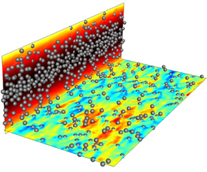
Visualizations of instantaneous fields from the Newtonian (W0P20) and viscoelastic (W25P20) particle-laden simulations are provided in figure 2, and serve to highlight the striking differences between the two conditions: in the viscoelastic case, the streamwise fluid velocity is appreciably higher in the channel centre, as shown by contours of instantaneous  $u_f$ (vertical planes) and by the mean velocity profiles. Furthermore, contours of
  $u_f \text {--} \langle u_f \rangle$ (horizontal planes) show that the turbulence motion is highly subdued by viscoelasticity. Also, the accumulation of particles in the centre of the channel in the viscoelastic condition is a signature of their migration. In the following, we extensively analyse the state of the flow, polymers and particles in order to explain the origins of these contrasting features.

Figure 2. Instantaneous particles positions and contours of (side view)  $u_f$ and (top view at
  $y=d_p$)
  $u_f\text {--}\langle u_f \rangle$ for (a) Newtonian case W0P20; (b) viscoelastic case W25P20. For clarity, only particles that are cut by the planes are displayed. Isosurfaces mark (a)
  $u\text {--}\langle u_f\rangle = \pm 0.2$ and (b)
  $u\text {--}\langle u_f\rangle = \pm 0.08$ in a subregion above the horizontal plane. Wall-normal profiles of the mean streamwise fluid velocity are also schematically displayed.
3.1. Drag modulation and stress balance
The fluid viscosity, turbulence, polymers and particle phase all contribute to the total stress within the channel. In order to assess their relative contributions, the mean total stress  $\tau _{tot}$ can be expressed in terms of its constituents,
 \begin{align} &\overbrace{\dfrac{\beta}{Re} (1-\phi) \dfrac{\boldsymbol{\text{d}}{\langle u_f \rangle}}{\text{d}{y}}}^{\displaystyle\tau_{\mu}} \
\overbrace{-[(1-\phi) \langle u'_f v'_f \rangle + \phi \langle u'_p v'_p \rangle]}^{\displaystyle\tau_{Re}} \nonumber\\
&\quad + \underbrace{\dfrac{(1-\beta)}{Re}(1-\phi) \langle \boldsymbol{\mathsf{T}}_{xy} \rangle}_{\displaystyle\tau_{\beta}} +
\underbrace{\phi \langle \sigma_{p,xy} \rangle}_{\displaystyle\tau_{\phi}} =
\underbrace{\langle \tau_{w}\rangle(1-y)}_{\displaystyle\tau_{tot}}. \end{align}
\begin{align} &\overbrace{\dfrac{\beta}{Re} (1-\phi) \dfrac{\boldsymbol{\text{d}}{\langle u_f \rangle}}{\text{d}{y}}}^{\displaystyle\tau_{\mu}} \
\overbrace{-[(1-\phi) \langle u'_f v'_f \rangle + \phi \langle u'_p v'_p \rangle]}^{\displaystyle\tau_{Re}} \nonumber\\
&\quad + \underbrace{\dfrac{(1-\beta)}{Re}(1-\phi) \langle \boldsymbol{\mathsf{T}}_{xy} \rangle}_{\displaystyle\tau_{\beta}} +
\underbrace{\phi \langle \sigma_{p,xy} \rangle}_{\displaystyle\tau_{\phi}} =
\underbrace{\langle \tau_{w}\rangle(1-y)}_{\displaystyle\tau_{tot}}. \end{align}
From left to right, the components are the viscous stress  $\tau _\mu$, the turbulent Reynolds stress
  $\tau _{Re}$, the polymer stress
  $\tau _\beta$ and the particle stress
  $\tau _\phi$. When integrated over
  $0<y<1$ and normalized by
  $0.5\langle \tau _{w} \rangle ^{{\text {W0}}}$ from the single-phase Newtonian case, the right-hand side of (3.1) reduces to
  $\langle \tau _{w} \rangle /\langle \tau _{w} \rangle ^{{\text {W0}}}$, i.e. the normalized mean wall shear stress (drag), and the left-hand side expresses the contribution of different stress constituents. Figure 3 reports the normalized total drag (height of the bars) and its constituents (layering of the bars) from the various flow conditions. While the primary focus of the present work is on dense concentration (
 $\varphi = 20\,\%$), for the purpose of comparison two dilute cases (
 $\varphi = 5\,\%$) from Esteghamatian & Zaki (Reference Esteghamatian and Zaki2019) are also included.

Figure 3. Contributions of different stress components to the total drag, integrated between  $0<y<1$ and normalized by
  $0.5\langle \tau _{w} \rangle ^{{\text {W0}}}$. Results are arranged to display the effect of (a) Weissenberg number, (b) solid volume fraction. The intensity of fluctuations of the total stress in time, measured by the standard deviation of
  $\langle \tau _{w} \rangle _{xz}/\langle \tau _{w} \rangle ^{{\text {W0}}}$, is shown by uncertainty bars. Case designations are listed in table 1.
We first focus on the effect of the Weissenberg number (figure 3a). In single-phase flows, with increasing viscoelasticity, the Reynolds shear stress markedly diminishes while the polymer stress is marginally enhanced. The net effect is the well-established reduction in the total drag. At  $20\,\%$ particle concentration, increasing viscoelasticity results in the reduction of the Reynolds shear stress, a mild increase in the particle stress and significant enhancement of the polymer stress.
These combined effects give rise to a non-monotonic behaviour in the total stress: the drag is decreased with an increase in viscoelasticity up to the point where the Reynolds shear stress is nearly eradicated in case W5P20. Beyond  $Wi=5$, further increasing
  $Wi$ only enhances the polymer and particle stresses and, in turn, the total drag.
The non-monotonic trend is not universal for all particle concentrations. Results from the earlier study at  $5\,\%$ particle concentration (Esteghamatian & Zaki Reference Esteghamatian and Zaki2019) predicted smaller particle and polymer stresses and lower drag relative to the
  $20\,\%$ cases, and a consistent reduction in the total stress with increasing elasticity. The Reynolds stress,
  $\tau _{Re}$, was also eradicated in the dilute case, but only at the highest Weissenberg number (case W25P5) – an indication that turbulence inhibition in particle-laden viscoelastic flows is weaker at dilute conditions. A comparison of the drag makeup at both concentrations suggests that increasing the Weissenberg number beyond
  $Wi=25$ in the dilute case (
 $\varphi =5\,\%$) would enhance the polymer stress and potentially increase the total drag, although additional simulations at the lower concentration would be required to verify this outcome. Nonetheless, the general conclusion is that increasing
  $Wi$ in particle-laden flows reduces drag when the reduction in
  $\tau _{Re}$ is appreciable, and hence
  $\tau _{Re}$ must be finite.
The intensity of fluctuations of the total stress in time, measured by the standard deviation of  $\langle \tau _{w} \rangle _{xz}/\langle \tau _{w} \rangle ^{{\text {W0}}}$, is shown by uncertainty bars in figure 3. Strong fluctuations in time are a signature of intermittency, or the alternation of the turbulence between a hibernating and an active state – an effect that intensifies at higher
  $Wi$. In cases where the turbulence is eradicated, the intermittency thus vanishes. At
  $\varphi = 20\,\%$, the intermittency is most pronounced at
  $Wi=3$. The results highlight that intermittency sets in and is most pronounced at lower
  $Wi$ for larger particle concentrations.
Figure 3(b) draws the focus to the effect of the solid volume fraction on different components of the total stress. In both Newtonian and viscoelastic conditions, the addition of particles increases the total drag. In the Newtonian cases, underlying the increase in total drag is a non-monotonic behaviour of the Reynolds stress: as the particle concentration is increased,  $\tau _{Re}$ first increases (W0P5) and then reduces (W0P20) relative to the single-phase configuration. This trend is consistent with a previous study in Newtonian flows and similar conditions by Picano et al. (Reference Picano, Breugem and Brandt2015). The increase in the total drag at higher particle concentration is more pronounced for the viscoelastic conditions due to the significant increase of the particle and polymer stresses with the solid volume fraction. Also, the non-monotonic trend in the Reynolds stress reported for Newtonian carrier fluids disappears in the viscoelastic cases: the addition of particles monotonically reduces and ultimately eliminates
  $\tau _{Re}$.
The particle stress  $\tau _\phi$ makes an important contribution to the total drag at
  $\varphi = 20\,\%$, and warrants consideration. Two relevant quantities are the solid volume fraction
  $\phi$ and the mean shear rate
  $\dot {\gamma } \equiv {\boldsymbol {\text {d}}{\langle u_f \rangle }}/{\text {d}{y}}$ (figure 4a,b). For
  $Wi\ge 5$, particles migrate away from the wall in all the particle-laden cases and the solid volume fraction reaches near
  $45\,\%$ at the channel centre (figure 4a) – an explanation of this migration trend is provided in § 3.4. In all cases, the
  $\phi$ profile has a local maximum near
  $y\approx d_p$, due to the asymmetric interaction of near-wall particles that are stabilized by the wall lubrication. For
  $Wi \geq 5$, a second local maximum near
  $y\approx 2d_p$ is indicative of a propensity for the particles to form a layered structure in the absence of a vertical mixing mechanism. The mean shear rate (figure 4b) exhibits a non-monotonic behaviour with increasing viscoelasticity. At the wall, it decreases to a minimum at
  $Wi=5$ and increases beyond that value. Away from the wall,
  $y \ge 0.2$, that trend is reversed and the mean shear rate is the highest for
  $Wi=5$ and decreases at higher
  $Wi$.
$Wi$.

Figure 4. Wall-normal profiles of (a) solid volume fraction; (b) mean shear rate  $\dot {\gamma } \equiv {\boldsymbol {\text {d}}{\langle u_f \rangle }}/{\text {d}{y}}$ in particle-laden cases; (c) particle stress
  $\tau _\phi$; and polymer stress
  $\tau _\beta$ in (d) single-phase and (e) particle-laden conditions. Line types are listed in table 1.
The profile of  $\tau _\phi$ (figure 4c) is influenced by viscoelasticity in three ways. (i) The polymers directly increase the stresslet contribution to the particle stress by altering the surface traction (Einarsson et al. Reference Einarsson, Yang and Shaqfeh2018). (ii) The mean shear rates are higher in the region
  $y\ge 0.2$. Since particles resist deformation under shear, the stresslet contribution to the particle stress is enhanced in that region. (iii) Due to the migration of particles towards the channel centre, the particle concentration and in turn the particle stress are larger at
  $y\geq 0.65$. A combination of all these effects leads to the larger particle stresses in the viscoelastic cases away from the wall. Near the wall, local peaks in
  $\tau _\phi$ coincide with the local maxima in the solid volume fraction. In addition, conditions with the stronger near-wall shear rates (
 $Wi<5$ cases) have larger peaks in the particle stress profiles.
The other important contribution to drag in the particle-laden viscoelastic cases is the polymer stress, especially when compared with the single-phase cases (figures 4d and 4e). The latter sustain small levels of  $\tau _\beta$, with very weak variation in the wall-normal direction. In contrast, in presence of the particle phase, the polymer stress increases appreciably, is highest in the near-wall region where particle layering is observed, and decays to zero towards the channel centre. Evidently, the particles contribute to the deformation of polymers and, in turn, increasing the polymer stress. It is unexpected, however, that the polymer stress vanishes in the region where the particles are most accumulated (
 $0.8 < y < 1.0$). In this region, the mean flow is akin to a plug profile with negligible shear rate due to the high concentration of particles (see figure 4b for the shear rate). This observation underscores that the presence of particles and of a finite shear rate are two essential components for effective polymer deformation. The differences between the polymer conformation in the near-wall region and the channel centre are further examined in § 3.3.
3.2. Flow structures and statistics
In this section, we examine the effect of particles on turbulent structures, mean flow statistics and Reynolds stresses. Figure 5 compares the instantaneous contours of  $u_f - \langle u_f \rangle$, and the correlation of
  $u'_f$ in the spanwise direction,
 \begin{equation} R_{u'_fu'_f}(y, {\rm \Delta} z) = \dfrac{\langle u'_f(x,y,z,t)u'_f(x,y,z+{\rm \Delta} z,t)\rangle}{ \langle u'_f(x,y,z,t)u'_f(x,y,z,t)\rangle}. \end{equation}
In single phase, relative to the Newtonian streaks, viscoelasticity inflates these structures (see figures 5a and 5b). Addition of particles to a Newtonian flow also increases the width of the streamwise structures (figure 5c). The particle-laden viscoelastic case is markedly different: the classical turbulent streaks are nearly absent at  $Wi =25$ (figure 5d), and the spanwise correlation length reduces to the order of a particle diameter.

Figure 5. Instantaneous contours and isosurfaces of  $u_f\text {--}\langle u_f\rangle$ and particle positions in
  $xz$ plane (top); and two-point correlation of
  $u'_f$ as a function of spanwise spacing (bottom). (a) Single-phase Newtonian (W0); (b) single-phase viscoelastic (W25); (c) particle-laden Newtonian (W0P20); (d) particle-laden viscoelastic (W25P20). The wall-normal location of the contours and correlations is
  $y u_\tau /\nu \approx 20$.
The mean fluid-velocity profiles and their deviation from Poiseuille flow are reported in figure 6. In single-phase flows, the mean profiles monotonically approach the Poiseuille condition with increasing elasticity. In particle-laden flows, a non-monotonic behaviour that is consistent with the change in drag is observed: the flow approaches the laminar condition with increasing elasticity up to  $Wi=5$ at which the turbulence is completely eradicated. Beyond that level, the polymer stress dominates the momentum transfer in the wall-normal direction. As a result, the mean velocity profiles are flattened with further increase in elasticity.

Figure 6. Mean streamwise fluid velocity (top); and its deviation from the laminar profile  $u_{{L}}$ (bottom) in (a) single-phase and (b) 20 % particle concentration. Line types are listed in table 1.
The normal components of the Reynolds stress tensor are plotted in figure 7. In single-phase flows, the peak of  $\langle u'_f u'_f \rangle$ shifts away from the wall with increasing elasticity due to the swelling of the streamwise streaks, and the stresses in the cross-flow plane are progressively attenuated at higher
  $Wi$. In particle-laden conditions, the co-presence of the solid phase and elasticity effectively suppresses the turbulent fluctuations. At
  $Wi\ge 5$, fluctuations are significantly suppressed in all three directions and become independent of elasticity. This observation reinforces our previous interpretation of flow perturbations (figure 5): they are not due to conventional turbulent eddies, but rather fluctuations due to the particles in shear.

Figure 7. Wall-normal profiles of (a,d) streamwise, (b,e) wall-normal and (c,f) spanwise fluid velocity fluctuations. Line types are listed in table 1.
Quadrant analysis of the Reynolds shear stress is reported in figure 8. The second and fourth quadrants ( $\langle u'_f v'_f \rangle _\text {Q2}$ and
  $\langle u'_f v'_f \rangle _\text {Q4}$) are associated with ejections and sweeps that are responsible for the turbulence production, while
  $\langle u'_f v'_f \rangle _\text {Q1}$ and
  $\langle u'_f v'_f \rangle _\text {Q3}$ correspond to interaction events that counter the wall-normal momentum flux (Wallace, Eckelmann & Brodkey Reference Wallace, Eckelmann and Brodkey1972). In single-phase flows, elasticity reduces the magnitude of
  $u_f'v_f'$ in all quadrants, while the largest drops are associated with
  $\langle u'_f v'_f \rangle _\text {Q2}$ and
  $\langle u'_f v'_f \rangle _\text {Q4}$. As a result, the net effect is a reduction in the turbulent shear stress and in turn the wall-normal momentum transfer.

Figure 8. Quadrant analysis of the Reynolds shear stress,  $\langle u'_f v'_f \rangle$, in (a) single-phase and (b) particle-laden conditions. Line types are listed in table 1.
The addition of particles to the Newtonian flow increases the contributions in  $\langle u'_f v'_f \rangle _\text {Q1}$,
  $\langle u'_f v'_f \rangle _\text {Q3}$ and
  $\langle u'_f v'_f \rangle _\text {Q4}$, while weakening
  $\langle u'_f v'_f \rangle _\text {Q2}$ ejection events. These modifications are marginal, and their net effect is an
  $11\,\%$ reduction in the turbulent shear stress relative to the single-phase condition. At
  $Wi=\{1,3\}$ the turbulence is still active, and the addition of particles results in
  $\{15,31\}\%$ decrease in the turbulent shear stress mostly due to weakened
  $\langle u'_f v'_f \rangle _\text {Q2}$ ejection events. Beyond
  $Wi = 5$, a steep reduction in the contributions to
  $\langle u'_fv'_f\rangle$ is observed in all four quadrants. The nearly symmetric contributions of
  $\langle u'_f v'_f \rangle _\text {Q1}$ to
  $\langle u'_f v'_f \rangle _\text {Q4}$ highlights that the turbulence production is completely disrupted. Also, the remarkable drop in the peak values underlines the reduction in correlated motions in the
  $x$ and
  $y$ directions.
3.3. Polymer conformation
Velocity gradients in the fluid phase, whether induced by the mean shear, turbulent fluctuations or particles, modify the polymer conformation away from equilibrium. As explained in detail by Hameduddin et al. (Reference Hameduddin, Meneveau, Zaki and Gayme2018), these modifications cannot be accurately interpreted with reference to isolated components of  $\boldsymbol{\mathsf{c}}$. Instead, those authors introduced three rigorous measures to characterize the conformation tensor and its perturbations: (i) the logarithmic volume ratio,
  $\log (\det (\boldsymbol{\mathsf{c}})/\det (\bar {\boldsymbol{\mathsf{c}}}))$, which compares the volume of the instantaneous polymer conformation
  $\boldsymbol{\mathsf{c}}$ relative to a reference conformation tensor
  $\bar {\boldsymbol{\mathsf{c}}}$; (ii) the squared geodesic distance between
  $\boldsymbol{\mathsf{c}}$ and
  $\bar {\boldsymbol{\mathsf{c}}}$ on the manifold of positive-definite matrices; (iii) the anisotropy which is a function of (i) and (ii), and therefore is not considered in the present study. The squared geodesic distance between a pair of positive-definite matrices
  ${\boldsymbol{\mathsf{A}}}$ and
  ${\boldsymbol{\mathsf{B}}}$ is defined by
 \begin{equation} \textrm{d}^2({\boldsymbol{\mathsf{A}}},{\boldsymbol{\mathsf{B}}}) \equiv \text{tr}(\log^2({\boldsymbol{\mathsf{A}}}^{-1/2} \boldsymbol{\cdot} {\boldsymbol{\mathsf{B}}} \boldsymbol{\cdot} {\boldsymbol{\mathsf{A}}}^{-1/2})) . \end{equation}
 Wall-normal profiles of the first two scalar measures are reported in figure 9, where the reference tensor was selected to be  $\bar {\boldsymbol{\mathsf{c}}} = \boldsymbol{\mathsf{I}}$ in order to highlight the departure of the polymer from the isotropic equilibrium state. This choice of the reference state also affords a fair comparison across the different flow configurations. In both the single-phase and particle-laden cases,
  $\langle \log (\det (\boldsymbol{\mathsf{c}}))\rangle$ and
  $\langle \textrm {d}^2(\boldsymbol{\mathsf{I}},\boldsymbol{\mathsf{c}}) \rangle$ increase with
  $Wi$, with marginal difference between
  $Wi = 15$ and
  $Wi=25$. In single-phase flows, and at the lowest
  $Wi$, the profiles of both measures decay in the outer flow due to the fast polymer relaxation away from the peak turbulence production. At the higher
  $Wi$ cases, the profiles only have weak variations in the wall-normal direction. Due to the long polymers’ relaxation times in these cases, the perturbations in polymer conformations are effectively transported by turbulent motion across the channel, explaining the almost uniform profile of both measures in the bulk of the channel at
  $Wi=\{15,25\}$. In the particle-laden cases with
  $Wi \ge 5$, the wall-normal mixing is inhibited due to the suppression of turbulence (cf. figure 8b), yet both measures still exhibit small variations in most of the channel, except near the centre. The controlling factors in polymer perturbations in particle-laden cases with
  $Wi \ge 5$ are the mean shear rate and the particle concentration. From the wall to the centre, the polymer perturbation is enhanced with an increase in the number of particles, yet hindered by a decrease in the mean shear rate. These competing effects explain the weak variations in most of the channel. Nevertheless, near the channel centre where the mean shear decays to zero and the particles population is the highest, the significant drop in both measures of polymer deformation is a signature of a different particle–polymer interaction mechanism, which is further detailed in the following.

Profiles of  $\langle \textrm {d}^2(\langle \boldsymbol{\mathsf{c}} \rangle _{\log },\boldsymbol{\mathsf{c}}) \rangle$ are reported for the single-phase and particle-laden conditions in figure 10. This quantity is the average of the squared geodesic distance between the instantaneous and the log-Euclidean mean conformation, and is therefore a measure of the intensity of the perturbation from that mean at different
  $y$ locations. Note that since volumetric compressions and expansions of polymers with respect to
  $\langle \boldsymbol{\mathsf{c}} \rangle _{\log }$ are symmetric, the average value of
  $\log (\det (\boldsymbol{\mathsf{c}})/\det (\langle \boldsymbol{\mathsf{c}} \rangle _{\log }))$ is zero and is therefore not reported. In the single-phase flows, higher elasticity is associated with larger departures of the conformation from its mean value, and the profiles of
  $\langle \textrm {d}^2(\langle \boldsymbol{\mathsf{c}} \rangle _{\log },\boldsymbol{\mathsf{c}}) \rangle$ become nearly flat for
  $Wi \geq 5$. The recorded values are, as can be anticipated, smaller than
  $\langle \textrm {d}^2(\boldsymbol{\mathsf{I}}, \boldsymbol{\mathsf{c}}) \rangle$. Another notable difference is the appreciable near-wall drop in figure 10(a) relative to figure 9(c): although the polymers are highly deformed in the near-wall region, the fluctuations away from their log-Euclidean mean are relatively small. In the particle-laden cases, local maxima near the wall coincide with the peaks of the solid volume fraction profiles (cf. figure 4a). In the outer bulk flow, where the particle population is larger, the perturbations relative to the mean are enhanced at larger
  $Wi$. Nevertheless, in all cases the fluctuations decay significantly beyond
  $y \approx 0.8$, confirming the trends in the profiles of
  $\langle \log (\det (\boldsymbol{\mathsf{c}}))\rangle$ and
  $\langle \textrm {d}^2(\boldsymbol{\mathsf{c}}, \boldsymbol{\mathsf{I}}) \rangle$ in figures 9(b) and 9(d).

Figure 10. Wall-normal profiles of the mean squared geodesic distance between instantaneous and the log-Euclidean mean conformation tensors in (a) single-phase and (b) particle-laden conditions. Line types are listed table 1.
We now direct the focus to select  $y$ locations where we provide a further detailed account of the polymer deformation when
  $Wi=25$; the results for
  $Wi=15$ are qualitatively similar. Figure 11 shows the joint probability density function (JPDF) of
  $\langle \textrm {d}^2(\boldsymbol{\mathsf{I}}, \boldsymbol{\mathsf{c}}) \rangle$ and
  $\log (\det (\boldsymbol{\mathsf{c}}))$. At
  $y=0.15$, polymers depart appreciably from the isotropic state and, in the particle-laden condition, are more deformed and expanded compared with the single-phase counterpart (figure 11a). The figure also shows instantaneous realizations of the polymer conformation, visualized using ellipsoids whose axes are the eigenvectors of the tensor each scaled by the corresponding eigenvalues; the ellipsoid are also coloured by the logarithm of the volume of the tensor. These visualizations suggest dissimilar mechanisms for polymers’ deformation in the single-phase and particle-laden cases. In the former, polymers are most perturbed in the vicinity of the coherent turbulent structures, visualized by contours of
  $u_f\text {--}\langle u_f \rangle$. On the other hand, in the particle-laden condition, large polymer deformation are observed in the vicinity of particles. The JPDF of
  $\langle \textrm {d}^2(\boldsymbol{\mathsf{I}}, \boldsymbol{\mathsf{c}}) \rangle$ and
  $\log (\det (\boldsymbol{\mathsf{c}}))$ at the channel centre (figure 11b) shows appreciable departure of the polymer from equilibrium in the single-phase condition. In contrast, in the particle-laden case the polymer conformation is most akin to the isotropic equilibrium state.

Figure 11. The JPDF of squared geodesic distance  $\textrm {d}^2(\boldsymbol{\mathsf{I}},\boldsymbol{\mathsf{c}})$ and the logarithmic volume
  $\log (\det (\boldsymbol{\mathsf{c}}))$ at (a)
  $y=0.15$ and (b)
  $y = 1$. Flood (particle-laden) and line (single-phase) contours are plotted in the same range, and refer to the cases with the
  $Wi=25$ condition. Flow visualizations show snapshots of
  $u_f\text {--}\langle u_f \rangle$ contours in the single-phase condition and position of particles that are cut by the
  $x$–
$x$– $z$ plane in the particle-laden case. The ellipsoids represent instantaneous realizations of the polymer conformation, are coloured by the logarithmic volume of
  $\boldsymbol{\mathsf{c}}$, and their axes are the eigenvectors of
  $\boldsymbol{\mathsf{c}}$ scaled by the corresponding eigenvalues.
The instantaneous visualizations at  $y=1$ show that the polymer conformation is relatively small in volume in the two-phase case, in the confined regions between the crowd of particles. Scattered instances of deformed polymer conformation are still observable, although their presence is rare and their magnitude is small (note that the colourbars for
  $\log (\det (\boldsymbol{\mathsf{c}}))$ in the particle-laden condition have different ranges in figures 11a and 11b).
So far, we have shown that the particles appreciably alter the polymer deformation and, in turn, the associated stresses. We will now examine how these deformations take place at the particle scale. To this end, we first describe the particles’ microstructure by evaluating the particle-pair distribution function,  $q(r,\psi ,\theta )$, which depends on the pair separation
  $r$, the polar angle
  $\psi$ relative to the positive
  $z$ axis, and the azimuthal angle
  $\theta$ measured anticlockwise from the positive
  $x$ axis,
 \begin{gather} q(r,\psi,\theta) = \langle \text{d}N(r,\psi,\theta) \rangle / \langle \text{d} N(r,\psi,\theta)^{R} \rangle, \end{gather}
 \begin{gather}\text{d}N(r,\psi,\theta) = \sum_{m=1}^{N_p} \delta(r-|{\boldsymbol{r}}_{m}|)\delta(\psi - \psi_{m})\delta(\theta - \theta_{m}), \end{gather}
 \begin{gather}{\boldsymbol{r}}_{m} = {\boldsymbol{P}}_{m} - {\boldsymbol{P}}_{ref}, \end{gather}
 \begin{gather}\psi_{m} = \cos^{-1}\left(\dfrac{{\boldsymbol{r}}_m\boldsymbol{\cdot} \boldsymbol{e}_z}{|{\boldsymbol{r}}_{m}|} \right); \quad \theta_{m} = \arctan\left(\dfrac{{\boldsymbol{r}}_m\boldsymbol{\cdot} \boldsymbol{e}_y}{{\boldsymbol{r}}_m\boldsymbol{\cdot} \boldsymbol{e}_x}\right). \end{gather}
The number of neighbouring particles within each bin is denoted  $\text {d}N$, and
  ${\boldsymbol {P}}$ refers to the particles’ position vector. Similar to our previous study (Esteghamatian & Zaki Reference Esteghamatian and Zaki2019), the particle-pair distribution function
  $q$ is normalized by
  $\textrm {d}N^R$ which corresponds to a random distribution of particles with a no-overlap condition and the case-specific wall-normal profile of the mean solid fraction, in order to eliminate bias in the interpretation of the results.
Results for reference particles located at  $y=0.2$ are shown in figure 12(a). Contours of
  $q(r = 1.05d_p)$ are projected onto the particle surface. In terms of the particle-attached coordinates,
  $\tilde {{\boldsymbol {x}}}=\boldsymbol {x} - {\boldsymbol {P}}_{ref}$, the pairwise distribution function shows accumulations of neighbouring particles in the regions
  $\tilde {x}\tilde {y}<0$ and depletion
  $\tilde {x}\tilde {y}>0$. This microstructure is generally observed when finite-size particles are suspended in shear flows: particles at
  $\tilde {y}>0$ advect faster than the reference one and, as a result, are more likely to accumulate behind it. A similar explanation describes the asymmetry of
  $q$ with respect to the
  $\tilde {y}$ axis at
  $\tilde {y}<0$ locations, where the neighbouring particles advect more slowly than the reference one.

Figure 12. Particle-pair distribution and polymer conformation for case W25P20. (a) Reference particle located at  $y=0.2$ coloured by
  $q(r = 1.05d_p)$. Ellipsoids represent the particle-conditioned log-Euclidean mean conformation
  $\langle \boldsymbol{\mathsf{c}} \rangle _{\log }$ coloured by their logarithmic volume and plotted in the particle coordinates (
 $\tilde {\boldsymbol {x}}=\boldsymbol {x} - \boldsymbol {P}_{ref}$). Four regions within one diameter from the particle centre are designated
  $\Omega _1$–
 $\Omega _4$. (b) The JPDF of squared geodesic distance
  $\textrm {d}^2(\langle \boldsymbol{\mathsf{c}} \rangle _{\log },\boldsymbol{\mathsf{c}})$ and logarithmic volume ratio
  $\log (\det (\boldsymbol{\mathsf{c}})/\det (\langle \boldsymbol{\mathsf{c}} \rangle _{\log }))$ for points located at
  $y=0.15$ (
 $\tilde {y}=-0.05$). Line contours are unconditional; colours are points within one diameter of a particle centre and exclusively located in (left)
  $\Omega _1$ or
  $\Omega _3$ versus (right)
  $\Omega _2$ or
  $\Omega _4$.
Figure 12(a) also shows the conditionally averaged log-Euclidean polymer conformation  $\langle \boldsymbol{\mathsf{c}} \rangle _{\log }$. In order to aid the discussion, four regions are identified within one diameter of the particle centre and are designated
  $\Omega _1$ to
  $\Omega _4$. Regions
  $\Omega _1$ and
  $\Omega _3$ correspond to
  $\tilde { x} \tilde { y} > 0$, while
  $\Omega _2$ and
  $\Omega _4$ correspond to
  $\tilde { x} \tilde { y} < 0$. The conformation tensors have larger volumes in
  $\Omega _1$ and
  $\Omega _3$, where polymers are effectively deformed by the presence of the reference particle and unconstrained by adjacent particles, as demonstrated by the particles microstructure. In the other two regions, where the neighbouring particles are stabilized by collision, polymers are overall less deformed and large deformations are only recorded in the immediate vicinity of the reference particle.
The effect of the microstructure on the polymer conformation in case W25P20 is quantified using the JPDF of the squared geodesic distance and logarithmic volume ratio in figure 12(b). The adopted reference conformation is  $\bar {\boldsymbol{\mathsf{c}}} = \langle \boldsymbol{\mathsf{c}} \rangle _{\log }$, that is to say the polymer deformation is evaluated relative to the log-Euclidean mean conformation. The line contours in both panels show the unconditional JPDF at
  $y = 0.15$. Near symmetry of positive and negative values of the logarithmic volume ratio confirms that the log-Euclidean mean is representative of the ensemble. The colour contours display the JPDF conditional on the fluid points belonging to specific regions: the left panel for points in
  $\Omega _1$ and
  $\Omega _3$, and the right for points in
  $\Omega _2$ and
  $\Omega _4$. In both figures, the colour contours are skewed towards larger values of the logarithmic volume ratio, highlighting the role of particles in the deformation of the polymers. The shift of the peak in the JPDFs towards larger expansions and squared geodesic distances is more appreciable in
  $\Omega _1$ and
  $\Omega _3$, which is consistent with the interpretation of figure 12(a): polymers are more deformed in
  $\tilde {x}\tilde {y}>0$ regions, where the reference particle is not immediately constrained by immediate neighbours.
3.4. Particle dynamics: diffusion and migration
The diffusion of particles is examined by evaluating their mean square displacement in the wall-normal direction  $\langle {\rm \Delta} y^2\rangle$ as a function of the separation time
  ${\rm \Delta} t$:
 \begin{equation} \langle {\rm \Delta} y^2\rangle \equiv \langle (P_y(t+{\rm \Delta} t) - P_y(t))^2\rangle, \end{equation}
where the average is performed over the ensemble of particles which at time  $t$ are located in a wall-parallel bin centred at
  $y$. The extent of the bin in the wall-normal direction is
  $1.5d_p$, while in the
  $x$ and
  $z$ directions it spans the full domain. The mean square displacements as a function of
  ${\rm \Delta} t$ are reported in figure 13, and exhibit quadratic and linear growth at small and large separation times, respectively. The former is indicative of correlated motion driven by collisions, and the latter is due to uncorrelated diffusive motion. In viscoelastic conditions, the eradication of turbulence results in faster decorrelation of particles motion compared with the Newtonian flow. In addition, the mean square displacements are orders of magnitude smaller in the viscoelastic flow due to the weaker mixing of particles in the wall-normal direction.

Figure 13. Particles’ mean squared displacement in the wall-normal direction (cf. (3.8)) normalized by the particle diameter squared  $\langle {\rm \Delta} y^2 \rangle /d_p^2$, for cases (a) W0P20 and (b,c) W25P20. In panel (c), the ordinate is also normalized by the mean shear rate of the streamwise fluid velocity
  $\dot {\gamma }$. The colours indicate different
  $y$ locations of the reference particle at
  ${\rm \Delta} t = 0$.
In the Newtonian condition, the first bin for the computation of  $\langle {\rm \Delta} y^2\rangle$ is located at
  $y^+\approx 35$. At higher wall-normal positions, and during the correlated regime
  $\langle {\rm \Delta} y^2\rangle \propto {\rm \Delta} t^2$, the mean squared displacements weakly decrease as the turbulence activity decreases. In the viscoelastic flow,
  $\langle {\rm \Delta} y^2\rangle$ is a stronger function of
  $y$ during both the correlated and diffusive regimes. In the absence of the turbulence, it is expected that the particles’ dynamics is driven by shear-induced self-diffusion. We examine this hypothesis by normalizing
  $\langle {\rm \Delta} y^2\rangle$ with the mean shear rate of the streamwise fluid velocity,
  $\dot {\gamma }$, in figure 13(c). The better collapse of the curves corresponding to different
  $y$ locations confirms that the shear-induced self-diffusion is a dominant mechanism for the dispersion of particles in the wall-normal direction.
In § 3.1, we have shown that the particles’ concentration increases away from the wall for  $Wi \ge 5$ (cf. figure 4a). An explanation was sought by performing an additional simulation that probes the transient particles’ migration dynamics. The initial condition was a snapshot from the statistically stationary Newtonian particle-laden flow, where the particle concentration is almost flat in the majority of the channel. Viscoelasticity was then suddenly introduced, with
  $Wi=25$. The particles migrated towards the channel centre over approximately 400 time units, and the migration velocity progressively weakened. The equilibrium concentration profile for case W25P20 was established beyond
  $t=500$.
A particle in wall-bounded shear has an equilibrium position farther away from the wall when the carrier fluid is viscoelastic compared with Newtonian (e.g. Karnis & Mason (Reference Karnis and Mason1966); Leshansky et al. (Reference Leshansky, Bransky, Korin and Dinnar2007), and the Appendix). This lateral migration of isolated particles, or in the very dilute regime, is well documented and is due to an imbalance of elastic normal stresses (see D'Avino, Greco & Maffettone (Reference D'Avino, Greco and Maffettone2017), for a review). In the present concentrated suspension, interparticle collisions play an important role in shear-induced migration towards the channel centre. In order to elucidate the mechanism, the statistical measures introduced by Sundaram & Collins (Reference Sundaram and Collins1997) are tailored for our configuration. The propensity of particle interactions to affect a reference particle is determined by (i) the probability of the presence of a neighbouring particle and (ii) the intensity of their relative velocity. The first measure is quantified by the particle-pair distribution function, previously defined as  $q$ in (3.4). Here the quantity is redefined with a different normalization,
 \begin{equation} q'(r,\psi,\theta) = \langle \text{d}N(r,\psi,\theta) \rangle / (r^2\,\text{d}\theta \, \text{d}\psi \,\text{d}r), \end{equation}
namely using the volume of the spherical bin,  $r^2\,\text {d}\theta \,\text {d}\psi \,\text {d}r$. Unlike the previous definition,
  $q'(r,\psi ,\theta )$ is intentionally biased by the inhomogeneity of particles distribution in the wall-normal direction. As we will show shortly, this inhomogeneity plays an important role in the migration dynamics. The second measure is expressed by the approaching velocity between the reference and a neighbouring particle
  $m$,
$m$,
 \begin{gather} {\rm \Delta} u^{n,-} (r,\psi,\theta)= \dfrac{ \displaystyle\sum_{m=1}^{N_p} \delta(r-|{\boldsymbol{r}}_{m}|)\delta(\psi - \psi_{m})\delta(\theta - \theta_{m}) {\rm \Delta} u_{m}^{n,-}}{\text{d}N(r,\psi,\theta)}, \end{gather}
 \begin{gather}{\rm \Delta} u_{m}^{n,-}= \max\left\{0, -(\boldsymbol{u}_{p,m} - \boldsymbol{u}_{p,{ref}})\boldsymbol{\cdot} \dfrac{{\boldsymbol{r}}_m}{|{\boldsymbol{r}}_m|}\right\}. \end{gather}
On average,  $\langle {\rm \Delta} u^{n,-} \rangle (r,\psi ,\theta )$ describes the spatial variations in the approaching velocity of neighbouring particles in the vicinity of the reference one. Finally, the product of
  $q'$ and
  $\langle {\rm \Delta} u^{n,-} \rangle$, referred to as the collision kernel when
  $r=d_p$ (Sundaram & Collins Reference Sundaram and Collins1997), quantifies the intensity of collision events. Note that in addition to direct collisions, neighbouring particles also indirectly affect the motion of the reference one by displacement of the interstitial fluid between them. Hence, the observable
  $q' \times \langle {\rm \Delta} u^{n,-} \rangle$ will be examined even at
  $r>d_p$, with the knowledge that values at larger separation distances are less relevant to the dynamics of the reference particle.
These statistical measures are reported in figure 14 for case W25P20. The figure compares the initial transient of the simulation and a statistically stationary interval. During the former, the profile of solid volume fraction is similar to its initial condition adopted from the Newtonian flow, i.e. it increases away from the wall at a relatively weak rate compared with its statistically stationary state. As a result,  $q'$ is slightly larger above the reference particle than below it during the transient, and this asymmetry becomes much more pronounced in the statistically stationary state (figure 14a). Due to the positive mean shear rate, neighbouring particles experience a finite approaching velocity only in regions
  $\Omega _2$ and
  $\Omega _4$ (cf. figure 12a for a definition). Also, the values of
  $\langle {\rm \Delta} u_p^{n,-} \rangle$ are larger in
  $\Omega _4$ due to the curvature of the mean streamwise velocity profile: the mean shear rate decreases away from the wall, giving rise to a stronger approaching velocity for neighbouring particles below the reference one (figure 14b). The combination of these two effects is shown in figure 14(c). While in the statistically stationary state
  $q' \times \langle {\rm \Delta} u_p^{n,-} \rangle$ is symmetric about the origin, it is larger in
  $\Omega _4$ during the initial transient. Hence, stronger collisions from below drive the reference particle towards the channel centre. In short, the curvature in mean streamwise velocity profile induces the migration of particles towards the channel centre, and this effect is eventually counterbalanced by the gradient of solid volume fraction in the wall-normal direction.

Figure 14. Measures of microstructure for case W25P20 and particles located at  $0.6 \le y \le 0.8$, averaged during (top) transient and (middle) statistically stationary intervals. Lines compare the statistics averaged over
  $1\le r/d_p \le 2$. (a) Particle-pair distribution function
  $q'(r,\psi ,\theta )$ (3.9), (b) mean approaching velocity
  $\langle {\rm \Delta} u_p^{n,-}(r,\psi ,\theta ) \rangle$ (3.10) and (c) intensity of particles collision measured by
  $q'\times \langle {\rm \Delta} u_p^{n,-} \rangle$. All quantities are averaged over the polar angle range of
  $- {{\rm \pi} }/{8} < \psi - {{\rm \pi} }/{2} < {{\rm \pi} }/{8}$.
The results presented herein showed that, while both the presence of particles and viscoelasticity can suppress and even eradicate turbulence at moderate particle concentrations and high elasticity, drag can increase appreciably. Both the particle and polymer stresses become important in these conditions. The large contribution to the polymer stress takes place in the high-shear region of the flow, where the polymers undergo appreciable deformation in the vicinity of the particles, and decays in the channel centre. The particle contribution to the stress shifts away from the wall at higher  $Wi$ due to the change in the preferential migration of the particles.
4. Conclusion
Direct numerical simulations of particle-laden viscoelastic flow in a channel were performed at moderate particle concentration and a wide range of Weissenberg numbers, and the results were analysed in detail. The flow was resolved at the scale of particles with an immersed boundary method, and the viscoelastic effects were modelled by solving the evolution equations of the polymer conformation tensor for a FENE-P fluid. The particle-laden cases with a bulk solid volume fraction  $\varphi = 20\,\%$ were contrasted to their single-phase counterparts. Key features of the flow were also contrasted to data at dilute concentration (
 $\varphi = 5\,\%$) from a previous study (Esteghamatian & Zaki Reference Esteghamatian and Zaki2019); differences are striking all the way from the global stress balance and down to the particle migration and microstructure.
In a regime where single-phase and dilute two-phase viscoelastic flows exhibit drag reduction with increasing elasticity, the concentrated suspension of particles leads to a non-monotonic change in drag. At low Weissenberg numbers, the turbulent shear stress is effectively reduced along with the total drag. Beyond  $Wi=5$, turbulence is nearly eradicated and the drag increases with increasing elasticity, due primarily to an increasing contribution from the polymer stress.
Consistent with the change in drag, the mean flow approaches the Poiseuille profile as the Weissenberg number approaches  $Wi=5$. Beyond that level, in the particle-laden flows, the mean flow flattens with further increase in elasticity. While this effect is reminiscent of the transition from laminar to elasto-inertial turbulence in single-phase viscoelastic flows (Choueiri, Lopez & Hof Reference Choueiri, Lopez and Hof2018), turbulence does not play a role here. The diagonal components of the Reynolds stresses, although highly suppressed, are still finite and are primarily driven by particle-induced perturbations which are insensitive to the level of elasticity. In addition, the shear component of Reynolds stresses is nearly eradicated, and quadrant analysis shows that each quadrant has nearly equal contribution to
  $u'_fv'_f$.
The influence of particles on the polymer stresses is examined by comparing the deformation and expansion of polymers in the single-phase and particle-laden conditions. Following Hameduddin & Zaki (Reference Hameduddin and Zaki2019), special care is exercised in characterizing the mean and deformations of the conformation tensor.
In the single-phase flow polymers are deformed in regions of the flow with high turbulence activity, while in the particle-laden case the strong polymer deformations and expansions are recorded in the vicinity of the particles’ surfaces. By examining the particles microstructure, we showed that polymers are effectively perturbed in the straining regions near a reference particle, where the presence of neighbouring particles is less probable.
The dynamics of the particles was investigated by examining their diffusion and migration mechanism. Here too the findings are qualitatively different from the dilute case, where particles can promote the cycles of hibernating and active turbulence during which they synchronously migrate away from and towards the wall (Esteghamatian & Zaki Reference Esteghamatian and Zaki2019). In the present concentrated suspension and at the same level of elasticity, these cycles are entirely absent and the wall-normal particle mixing is markedly hindered due to the eradication of turbulence. A shear-induced self-diffusion is identified as the primary mechanism for mixing of particles in the viscoelastic conditions. In addition, transient migration towards the channel centre was observed exclusively in viscoelastic cases with  $Wi \ge 5$ condition. Theoretical studies generally ascribe such migration trend to an imbalance in the particle-phase normal stresses (Morris Reference Morris2009). We provided an explanation by comparing the microstructure and the collision statistics during the transient and statistically stationary stages of the simulations, starting from the Newtonian configuration and suddenly introducing viscoelasticity. The collision kernel shows that the curvature of the mean velocity profile leads to preferential migration towards the channel centre, which is counterbalanced by the gradient of solid volume fraction in the statistically stationary state.
Taken all together, at high elasticity and particle concentration, the migration pattern of the particles leads to clustering in the channel centre where the polymers in the interstitial space are inappreciably perturbed away from equilibrium. Yet, away from the channel centre, a significant increase in the polymer stresses is recorded near the particles’ surfaces and becomes sufficiently large at high elasticity to ultimately cause an increase in the total drag – a reversal in the commonly anticipated effect of polymers.
Acknowledgements
This work was supported in part by the National Science Foundation (grant 1804004). Computational resources were provided by the Maryland Advanced Research Computing Center (MARCC).
Declaration of interests
The authors report no conflict of interest.
Appendix. Validation of the numerical algorithm
The particle-laden viscoelastic solver was extensively validated (see Esteghamatian & Zaki Reference Esteghamatian and Zaki2019). An additional validation case is presented here, where the lateral migration of a sphere in Newtonian and Oldroyd-B fluids is simulated and compared with data by Li, McKinley & Ardekani (Reference Li, McKinley and Ardekani2015). The computational domain is a duct geometry as illustrated in figure 15. The flow is periodic in  $x$, and no-slip boundary conditions are imposed at
  $y=\{0,1\}$ and
  $z=\{0,1\}$. A neutrally buoyant sphere of diameter
  $d_p$ is initially located at
  $(0 \times 0.75 \times 0.5)H$, where
  $H$ is the height of the square channel. Computations were performed in a domain spanning over
  $16d_p$ and the particle blockage ratio is
  $d_p/H = 0.25$. The prescribed Reynolds number based on centre velocity is
  $Re_c \equiv U_cH/\nu = 18.9$, and the Weissenberg number and the viscosity ratio are
  $Wi_c = \lambda U_c/H$ and
  $\beta = 0.1$. The particles’ equilibrium positions
  $y_{eq}$ for three viscoelastic cases,
  $Wi_c = \{0.189, 0.567, 0.945\}$, are contrasted to the Newtonian condition in table 2. The results demonstrate the accuracy of our prediction of the particle migration and equilibrium condition.

Figure 15. Configuration of validation test: lateral migration of a sphere in duct flow of Newtonian and Oldroyd-B fluids. No-slip boundary conditions  $\boldsymbol {u}_f = 0$ are imposed at
  $y=\{0,1\}$ and
  $z=\{0,1\}$, and periodicity is enforced in the
  $x$ direction.
Table 2. Parameters of the simulations of isolated particle in duct flow and the final equilibrium positions.


