NOMENCLATURE
- a w
-
ducted propeller expansion ratio (a w = A e/A R)
- A e
-
area of the exit section of the duct
- A R
-
area of the propeller disc
- c root
-
blade root chord
- CP
-
propeller power coefficient (
 $C_P = {\displaystyle {P}/{\rho _\infty n^3 D^5}}$
)
$C_P = {\displaystyle {P}/{\rho _\infty n^3 D^5}}$
) - CT
-
propeller thrust coefficient (
$C_T = {\displaystyle {T}/{\rho _\infty n^2 D^4}}$
) - D
-
propeller diameter
- I
-
cost function [Eq. 9]
- J
-
Jacobian matrix, advance ratio (J = V ∞/(nD))
- K r, n
-
binomial coefficient
- M ∞
-
free-stream Mach number
- n
-
propeller rotational speed (revolutions per second)
- P
-
propeller power
- P
-
flow solution vector, primitive variables
- R
-
propeller radius
-
${{\bm R}}$
-
flow equation residual vector
- Re
-
Reynolds number (
$\text{Re}=V_{\rm tip} c_{\rm root}/\nu _\infty$
) - T
-
propeller thrust
- V
-
mesh cell volume
- V ∞
-
free-stream velocity
- V tip
-
blade tip velocity
-
${{\bm W}}$
-
flow solution vector, conservative variables


Greek Symbols
-
${{\bm \alpha }}$
-
design variables vector [Eq. 9]
- β
-
blade pitch angle
- θ
-
blade twist angle
-
${{\bm \lambda }}$
-
adjoint variable vector [Eq. 10]
- η
-
propeller propulsive efficiency (
$\eta = J\ {\displaystyle {C_T}/{C_P}}$
) - ν∞
-
free-stream kinematic viscosity
- ρ∞
-
free-stream density


Acronyms
- ADT
-
Alternating Digital Tree
- CFD
-
Computational Fluid Dynamics
- CFL
-
Courant–Friedrichs–Lewy
- CST
-
Class/Shape Transformation
- FGMRES-DR
-
Flexible Generalised Minimum Residual with Deflated Restarting
- GCG
-
Generalised Conjugate Gradient
- HAV
-
Hybrid Air Vehicles Ltd
- HMB
-
Helicopter Multi-Block
- HPC
-
High-Performance Computing
- IDW
-
Inverse Distance Weighting
- LTA
-
Lighter-Than-Air vehicle
- NS
-
Navier-Stokes
- RANS
-
Reynolds-Averaged Navier-Stokes
- SLSQP
-
Sequential Least-Squares Quadratic Programming
Subscripts
- ∞
-
free-stream value
- i,j, k
-
mesh cell indices
Superscripts
- n
-
time level
- T
-
matrix transpose operator
1.0 INTRODUCTION
Propellers are very efficient in generating propulsive forces for low-speed aircraft, such as Lighter-Than-Air vehicles (LTAs). Their performance can be augmented by enclosing them in ducts(Reference McCormick20), that drive the expansion of their wake, decreasing the final wake velocity and reducing the induced power. Moreover, ducts reduce noise emissions and protect the propeller blades. The ideal power reduction P ducted/P free (for a fixed thrust) due to the duct is given by momentum theory(Reference Pereira22) and is a function of the ratio a w between the area of the exit section of the duct A e and the propeller disc area A R (see Fig. 1):
 $$\begin{equation}
{\displaystyle \frac{P_{\rm ducted}}{P_{\rm free}}} = {\displaystyle \frac{1}{\sqrt{2 a_{\rm w}}}}
\end{equation}$$
$$\begin{equation}
{\displaystyle \frac{P_{\rm ducted}}{P_{\rm free}}} = {\displaystyle \frac{1}{\sqrt{2 a_{\rm w}}}}
\end{equation}$$
The higher the value of a w, the higher the power reduction. In reality, however, the value of a w is limited by the adverse pressure gradient inside the duct diffuser, where flow separation may also take place. It follows that accurate predictions of the propulsor aerodynamics require high-fidelity Computational Fluid Dynamics (CFD) to capture the complex propeller flow and the interaction between the propeller wake and the duct. The aerodynamic analysis and the optimisation of a ducted propeller using high-fidelity flow modelling are pursued in this paper.
A representative geometry of a ducted LTA propeller with 1.2m radius was provided by Hybrid Air Vehicles Ltd (HAV), which includes the rotor blades, the duct, the nacelle enclosing the piston engine and the cooling devices (see Fig. 2). The performance of this baseline design was studied by solving the Reynolds-Averaged Navier-Stokes (RANS) equations with the k-ω turbulence model(Reference Wilcox33) by means of the HMB3 flow solver(Reference Barakos, Steijl, Badcock and Brocklehurst4,Reference Steijl, Barakos and Badcock31) . The obtained numerical results were compared with experimental data available from static tests conducted by HAV on a dedicated test rig (see Fig. 3), and very good agreement was observed between the predicted and measured power and thrust.
Figure 1. Schematic of a ducted propeller.
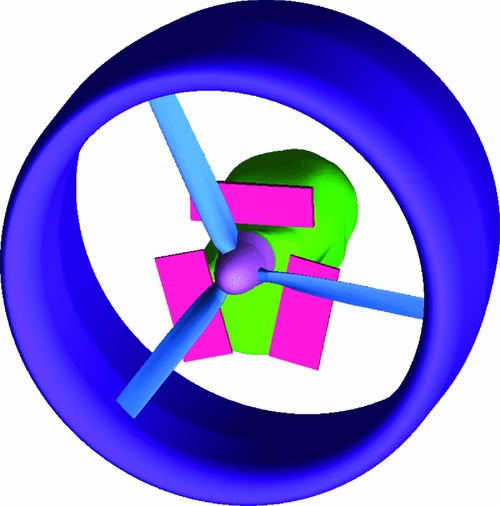
Figure 2. Ducted propeller with nacelle, radiators and cooler.

Figure 3. Propulsor test rig (Source Hybrid Air Vehicles Ltd).
The CFD model for the detailed geometry of the propulsor is, however, computationally expensive. Therefore, a simplified geometry was also considered, where the cooling devices were removed and the engine nacelle was replaced by an axisymmetric body (Fig. 4). This simpler geometry was used to quantify the effect of the duct by comparing the predicted thrust and power consumption with those of the unducted (or ‘free’) propeller (Fig. 5). The results revealed that the duct led to a substantial power reduction in low-speed operations, which cover a significant part of the LTA flight envelope.
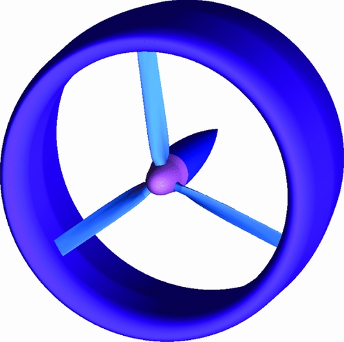
Figure 4. Ducted propeller.
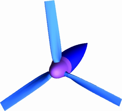
Figure 5. Free propeller.
The shape of the baseline rotor blade was optimised without the duct, and one question is whether this design is also optimal for the ducted configuration. This work focuses on the twist distribution, while other blade design parameters, such as aerofoils, chord distribution and sweep, are kept constant. To gain a basic understanding of the twist effect, the performance of the baseline blade, which is highly twisted, was compared with a low-twist blade. The low-twist blade design was the outcome of an optimisation study for low speeds, using a simple panel method(1). However, the high-fidelity CFD results presented in this paper show that the high-twist blade is superior at low and high speed.
An optimisation of the blade twist distribution with CFD was also attempted using the simplified geometry. The HMB3 flow solver was coupled with an external optimiser and an in-house parametrisation software for the blade surface. The computational mesh is updated at each optimisation cycle using an advanced deformation algorithm based on Inverse Distance Weighting (IDW)(Reference Shepard29). To minimise the expensive flow solution evaluations, a quasi-Newton optimisation method was employed. The optimiser used a Sequential Least-Squares Quadratic Programming (SLSQP) method(Reference Kraft17), as provided in the software library NLopt (Reference Johnson16). The required flow derivatives with respect to the design variables were computed using an implicit Fixed-Point Iteration (FPI) scheme(Reference Biava, Woodgate and Barakos6) or a recently developed Flexible Generalised Minimum Residual solver with Deflated Restarting (FGMRES-DR) nested with GMRES-DR (or standard GMRES) as a pre-conditioner(Reference Giraud, Gratton, Pinel and Vasseur13,Reference Morgan21,Reference Saad26) . While the FPI scheme has low memory usage, the FGMRES-DR method is more robust and faster to converge but more expensive in memory. The blade with optimised twist distribution has 1% higher propulsive efficiency with respect to the baseline design. The propulsive efficiency for the ducted propeller is defined as
 $$\begin{equation}
\eta = J {\displaystyle \frac{C_T}{C_P}},
\end{equation}$$
$$\begin{equation}
\eta = J {\displaystyle \frac{C_T}{C_P}},
\end{equation}$$
where the thrust coefficient CT includes the contribution of both the propeller and the duct. The reference area used for computing the coefficients is the propeller disc area, which is kept fixed throughout the optimisation process. To further increase the propulsor performance, the duct diffuser shape and dimensions were also considered for the optimisation, in addition to the twist distribution, and the resulting design has 2% more propulsive efficiency than the baseline.
The paper is structured as follows. Section 2 describes HMB3 and adjoint method, as well as the coupling strategy with the external optimiser. Section 3 presents the numerical results. The performance of the baseline propeller is firstly analysed with the detailed model, and a comparison with experimental data is presented. The effect of the duct and of the twist distribution is then assessed using the simplified geometry. The results of the twist and duct optimisations are finally presented. Conclusions are given in Section 4.
2.0 NUMERICAL METHODS
2.1 The optimisation tool chain
Gradient-based optimisation is an efficient and widely used method for aerodynamic shape optimisation problems, since it minimises the required number of flow solutions. It requires, however, the flow derivatives with respect to the design variables, which can be very expensive to compute when high-fidelity CFD is employed. An economic way to obtain the flow gradients with CFD is represented by the adjoint method, which reduces the cost of flow gradients evaluation to about twice the cost of the base flow solution, regardless of the number of design variables.
The HMB3 flow solver employs two adjoint solvers based on FPI scheme(Reference Biava, Woodgate and Barakos6) and FGMRES-DR(Reference Giraud, Gratton, Pinel and Vasseur13,Reference Morgan21) , which can be interfaced to any gradient-based optimisation tool to solve design problems. The current implementation employs a Sequential Quadratic Programming (SQP) optimisation algorithm(Reference Kraft17), as implemented in the software library NLopt (Reference Johnson16). It represents the objective function as a quadratic approximation to the Lagrangian and uses a dense SQP algorithm to minimise a quadratic model of the problem. It is intended for problems with up to a few hundred constraints and variables, since the required computer memory scales with the square of the problem dimension. The SQP algorithm is implemented in a separate tool, and it is interfaced with HMB3 using files for data exchange.
The mapping between the design space and the shape to be optimised is problem specific. In aerofoil design, usually a polynomial basis, such as Chebyshev or Bernstein polynomials, is used to represent the aerofoil. For three-dimensional objects (propeller blades, propulsor duct, etc.) more complex parametrisations may be required.
The design optimisation tool chain is described in Fig. 6 and can be summarised as follows.
-
1 The first step solves the flow around the baseline geometry of the shape under investigation (e.g. aerofoil, blade).
-
2 The cost functional I (e.g. drag to lift ratio, torque to thrust ratio) is evaluated from the flow solution.
-
3 The adjoint problem is solved to compute the gradient
$\text{d} I / \text{d} {{\bm \alpha }}$
of the cost functional with respect to the design variables vector
${{\bm \alpha }}$
. -
4 The cost functional and its gradient are fed to the gradient-based optimiser, which produces a new set of design variables, corresponding to a design candidate in the search direction.
-
5 An external parametrisation software updates the aerodynamic shape.
-
6 A mesh deformation algorithm computes the new volume mesh.
-
7 HMB3 solves the new flow problem and recomputes the cost functional I and its gradient
$\text{d} I / \text{d} {{\bm \alpha }}$
.


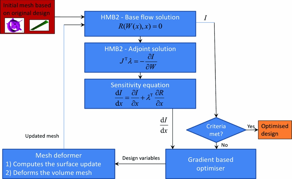
Figure 6. Flow chart of the optimisation process.
Steps 2-7 are repeated for several design cycles until determined convergence criteria are met.
2.2 The Flow Solver
The following contains a brief outline of the approach used in HMB3. The Navier-Stokes (NS) equations are discretised using a cell-centred finite-volume approach. The computational domain is divided into a finite number of non-overlapping control-volumes Vijk , and the governing equations are applied to each cell. Also, the NS equations are re-written in a curvilinear co-ordinate system which simplifies the formulation of the discretised terms since body-conforming meshes are adopted here. The spatial discretisation of the NS equations leads to a set of ordinary differential equations in real time:
 $$\begin{equation}
\frac{d}{dt} \left( {{{\bm W}}}_{ijk} V_{ijk} \right) = - {{{\bm R}}}_{ijk} \left( {{{\bm W}}} \right),
\end{equation}$$
$$\begin{equation}
\frac{d}{dt} \left( {{{\bm W}}}_{ijk} V_{ijk} \right) = - {{{\bm R}}}_{ijk} \left( {{{\bm W}}} \right),
\end{equation}$$
where
 ${{{\bm W}}}$
and
${{{\bm W}}}$
and
 ${{{\bm R}}}$
are the vectors of cell conserved variables and residuals, respectively. The convective terms are discretised using Osher’s upwind scheme(Reference Engquist and Osher11) for its robustness, accuracy and stability properties. Monotonic Upstream-Centred Scheme for Conservation Laws (MUSCL) variable extrapolation(Reference Hirsch14) is used to provide second-order accuracy with the Van Albada limiter(Reference Van Albada, Van Leer and Roberts32) to prevent spurious oscillations around shock waves. Alternatively, the classical Roe’s scheme(Reference Roe25), an all-Mach variant of the Roe’s scheme(Reference Rieper24), and the AUSM+ scheme(Reference Liou19), can be used. Boundary conditions are set using ghost cells on the exterior of the computational domain. At the far-field, ghost cells are set at the free-stream conditions. At solid boundaries, the no-slip condition is set for viscous flows.
${{{\bm R}}}$
are the vectors of cell conserved variables and residuals, respectively. The convective terms are discretised using Osher’s upwind scheme(Reference Engquist and Osher11) for its robustness, accuracy and stability properties. Monotonic Upstream-Centred Scheme for Conservation Laws (MUSCL) variable extrapolation(Reference Hirsch14) is used to provide second-order accuracy with the Van Albada limiter(Reference Van Albada, Van Leer and Roberts32) to prevent spurious oscillations around shock waves. Alternatively, the classical Roe’s scheme(Reference Roe25), an all-Mach variant of the Roe’s scheme(Reference Rieper24), and the AUSM+ scheme(Reference Liou19), can be used. Boundary conditions are set using ghost cells on the exterior of the computational domain. At the far-field, ghost cells are set at the free-stream conditions. At solid boundaries, the no-slip condition is set for viscous flows.
The integration in time of Equation (3) to a steady-state solution is performed using a fully implicit time-marching scheme by:
 $$\begin{equation}
\frac{{{{\bm W}}}_{ijk}^{n+1} - {{{\bm W}}}_{ijk}^n}{\Delta t} = - \frac{1}{V_{ijk}}{{{\bm R}}}_{ijk} \left( {{{\bm W}}}_{ijk}^{n+1} \right),
\end{equation}$$
$$\begin{equation}
\frac{{{{\bm W}}}_{ijk}^{n+1} - {{{\bm W}}}_{ijk}^n}{\Delta t} = - \frac{1}{V_{ijk}}{{{\bm R}}}_{ijk} \left( {{{\bm W}}}_{ijk}^{n+1} \right),
\end{equation}$$
where n + 1 denotes the real time (n + 1)Δt. For steady-state problems, the real time is replaced by a pseudo-time (τ), which is also used for unsteady problems according to the dual-time stepping scheme of Jameson(Reference Jameson15). Equation (4) represents a system of non-linear algebraic equations, and to simplify the solution procedure, the flux residual
 ${{{\bm R}}}_{ijk}( {{{\bm W}}}_{ijk}^{n+1})$
is linearised in time as follows:
${{{\bm R}}}_{ijk}( {{{\bm W}}}_{ijk}^{n+1})$
is linearised in time as follows:
 $$\begin{equation}
{{{\bm R}}}_{ijk} \left( {{{\bm W}}}^{n+1} \right) \approx {{{\bm R}}}_{ijk}^n \left( {{{\bm W}}}^{n} \right) + \frac{\partial {{{\bm R}}}_{ijk}}{\partial {{{\bm W}}}_{ijk}} \Delta {{{\bm W}}}_{ijk},
\end{equation}$$
$$\begin{equation}
{{{\bm R}}}_{ijk} \left( {{{\bm W}}}^{n+1} \right) \approx {{{\bm R}}}_{ijk}^n \left( {{{\bm W}}}^{n} \right) + \frac{\partial {{{\bm R}}}_{ijk}}{\partial {{{\bm W}}}_{ijk}} \Delta {{{\bm W}}}_{ijk},
\end{equation}$$
where
 $\Delta {{{\bm W}}}_{ijk}={{{\bm W}}}_{ijk}^{n+1}-{{{\bm W}}}_{ijk}^n$
. Equation (4) now becomes the following linear system:
$\Delta {{{\bm W}}}_{ijk}={{{\bm W}}}_{ijk}^{n+1}-{{{\bm W}}}_{ijk}^n$
. Equation (4) now becomes the following linear system:
 $$\begin{equation}
\left[\frac{V_{ijk}}{\Delta t} {\bf I} + \frac{\partial {{{\bm R}}}_{ijk}}{\partial {{{\bm W}}}_{ijk}} \right] \Delta {{{\bm W}}}_{ijk} = - {{{\bm R}}}_{ijk}^n \left( {{{\bm W}}}^n \right)
\end{equation}$$
$$\begin{equation}
\left[\frac{V_{ijk}}{\Delta t} {\bf I} + \frac{\partial {{{\bm R}}}_{ijk}}{\partial {{{\bm W}}}_{ijk}} \right] \Delta {{{\bm W}}}_{ijk} = - {{{\bm R}}}_{ijk}^n \left( {{{\bm W}}}^n \right)
\end{equation}$$
The left-hand side of Equation (6) is then rewritten in terms of primitive variables
 ${{{\bm P}}}$
:
${{{\bm P}}}$
:
 $$\begin{equation}
\left[ \left( \frac{V_{ijk}}{ \Delta t} \right) {\displaystyle \frac{\partial {{{\bm W}}}_{ijk}}{\partial {{{\bm P}}}_{ijk}}} + {\displaystyle \frac{\partial {{{\bm R}}}_{ijk}}{\partial {{{\bm P}}}_{ijk}}} \right] \Delta {{{\bm P}}}_{ijk} = - {{{\bm R}}}_{ijk}^n \left( {{{\bm W}}}^n \right)
\end{equation}$$
$$\begin{equation}
\left[ \left( \frac{V_{ijk}}{ \Delta t} \right) {\displaystyle \frac{\partial {{{\bm W}}}_{ijk}}{\partial {{{\bm P}}}_{ijk}}} + {\displaystyle \frac{\partial {{{\bm R}}}_{ijk}}{\partial {{{\bm P}}}_{ijk}}} \right] \Delta {{{\bm P}}}_{ijk} = - {{{\bm R}}}_{ijk}^n \left( {{{\bm W}}}^n \right)
\end{equation}$$
and the resulting linear system is solved with a Generalised Conjugate Gradient (GCG) iterative solver(Reference Axelsson3). Since at steady state the left-hand side of Equation (7) must be zero, the Jacobian
 $\partial {{\bm R}}/ \partial {{\bm P}}$
can be approximated by evaluating the derivatives of the residuals with a first-order scheme for the inviscid fluxes. The first-order Jacobian requires less storage and, being more dissipative, ensures a better convergence rate to the GCG iterations.
$\partial {{\bm R}}/ \partial {{\bm P}}$
can be approximated by evaluating the derivatives of the residuals with a first-order scheme for the inviscid fluxes. The first-order Jacobian requires less storage and, being more dissipative, ensures a better convergence rate to the GCG iterations.
The steady-state solver for turbulent flows is formulated and solved in an identical manner to that of the mean flow. The eddy-viscosity is calculated from the latest values of k and ω, for example, and is used to advance the mean and the turbulent flow solutions. An approximate Jacobian is used for the source term of the models by only taking into account the contribution of their dissipation terms, i.e. no account of the production terms is taken on the left-hand side of the system.
2.3 The adjoint solvers
An efficient way to compute the derivatives of the cost functional with respect to design variables is via solving the sensitivity equation casted in adjoint form. The underlying idea is to write explicitly the cost functional I as a function of the flow variables
 ${{\bm W}}$
and of the design variables
${{\bm W}}$
and of the design variables
 ${{\bm \alpha }}$
, that is,
${{\bm \alpha }}$
, that is,
 $I=I({{\bm W}}({{\bm \alpha }}),{{\bm \alpha }})$
. The flow variables are subject to satisfy the fluid dynamics governing equations (e.g. the NS equations) written in compact form as:
$I=I({{\bm W}}({{\bm \alpha }}),{{\bm \alpha }})$
. The flow variables are subject to satisfy the fluid dynamics governing equations (e.g. the NS equations) written in compact form as:
 $$\begin{equation}
{{\bm R}}({{\bm W}}({{\bm \alpha }}),{{\bm \alpha }}) = 0
\end{equation}$$
$$\begin{equation}
{{\bm R}}({{\bm W}}({{\bm \alpha }}),{{\bm \alpha }}) = 0
\end{equation}$$
Formally, taking the derivative of I with respect to
 ${{\bm \alpha }}$
, we obtain:
${{\bm \alpha }}$
, we obtain:
 $$\begin{equation}
{\displaystyle \frac{\text{d} I}{\text{d} {{\bm \alpha }}}} = {\displaystyle \frac{\partial I}{\partial {{\bm \alpha }}}} + {\displaystyle \frac{\partial I}{\partial {{\bm W}}}} {\displaystyle \frac{\partial {{\bm W}}}{\partial {{\bm \alpha }}}}
\end{equation}$$
$$\begin{equation}
{\displaystyle \frac{\text{d} I}{\text{d} {{\bm \alpha }}}} = {\displaystyle \frac{\partial I}{\partial {{\bm \alpha }}}} + {\displaystyle \frac{\partial I}{\partial {{\bm W}}}} {\displaystyle \frac{\partial {{\bm W}}}{\partial {{\bm \alpha }}}}
\end{equation}$$
By introducing the adjoint variable
 ${{\bm \lambda }}$
as the solution of the following linear system:
${{\bm \lambda }}$
as the solution of the following linear system:
 $$\begin{equation}
\left( {\frac{\partial {{\bm R}}}{\partial {{\bm W}}}} \right)^{\rm T} {{\bm \lambda }}= - \left( {\frac{\partial I}{\partial {{\bm W}}}} \right) ^{\rm T}
\end{equation}$$
$$\begin{equation}
\left( {\frac{\partial {{\bm R}}}{\partial {{\bm W}}}} \right)^{\rm T} {{\bm \lambda }}= - \left( {\frac{\partial I}{\partial {{\bm W}}}} \right) ^{\rm T}
\end{equation}$$
Equation (9) can be rewritten as:
 $$\begin{equation}
{\displaystyle \frac{\text{d} I}{\text{d} {{\bm \alpha }}}} = {\displaystyle \frac{\partial I}{\partial {{\bm \alpha }}}} + {{\bm \lambda }}^{\rm T} {\displaystyle \frac{\partial {{\bm R}}}{\partial {{\bm \alpha }}}}
\end{equation}$$
$$\begin{equation}
{\displaystyle \frac{\text{d} I}{\text{d} {{\bm \alpha }}}} = {\displaystyle \frac{\partial I}{\partial {{\bm \alpha }}}} + {{\bm \lambda }}^{\rm T} {\displaystyle \frac{\partial {{\bm R}}}{\partial {{\bm \alpha }}}}
\end{equation}$$
The computational cost of the dual-sensitivity problem (10)-(11) scales with the number of outputs, since the right-hand side of (10) depends on I, but it is independent of the input parameters. The adjoint form of the sensitivity equation is particularly efficient for cases where the number of (output) cost functionals is small, while the number of (input) design variables is large.
2.3.1 Fixed-point iteration scheme
The linear system (10) for computing the adjoint variable can be solved with a FPI scheme, where an approximation
 $\hat{J}$
of the linear system matrix J, with better condition number, is introduced as a pre-conditioner to advance the solution at each iteration(Reference Christianson10,Reference Giles, Corliss, Faure, Griewank, Hascoët and Naumann12) . The FPI scheme reads:
$\hat{J}$
of the linear system matrix J, with better condition number, is introduced as a pre-conditioner to advance the solution at each iteration(Reference Christianson10,Reference Giles, Corliss, Faure, Griewank, Hascoët and Naumann12) . The FPI scheme reads:
 $$\begin{equation}
\hat{J}^{\rm T} \Delta {{\bm \lambda }}^{n+1} = - \left( {\displaystyle \frac{\partial I}{\partial {{\bm W}}}} \right) ^{\rm T} - J^{\rm T} {{\bm \lambda }}^{n},
\end{equation}$$
$$\begin{equation}
\hat{J}^{\rm T} \Delta {{\bm \lambda }}^{n+1} = - \left( {\displaystyle \frac{\partial I}{\partial {{\bm W}}}} \right) ^{\rm T} - J^{\rm T} {{\bm \lambda }}^{n},
\end{equation}$$
where
 $$\begin{equation}
J = {\displaystyle \frac{\partial {{{\bm R}}}}{\partial {{{\bm W}}}}} , \\
\end{equation}$$
$$\begin{equation}
J = {\displaystyle \frac{\partial {{{\bm R}}}}{\partial {{{\bm W}}}}} , \\
\end{equation}$$
 $$\begin{equation}
\hat{J} = {\frac{V}{\text{CFL} \, \Delta t}} {{\bm I}}+ \left[ {\frac{\partial {{{\bm R}}}}{\partial {{{\bm W}}}}} \right] ^ {\rm 1st} , \\
\end{equation}$$
$$\begin{equation}
\hat{J} = {\frac{V}{\text{CFL} \, \Delta t}} {{\bm I}}+ \left[ {\frac{\partial {{{\bm R}}}}{\partial {{{\bm W}}}}} \right] ^ {\rm 1st} , \\
\end{equation}$$
 $$\begin{equation}
\Delta {{\bm \lambda }}^{n+1} = {{\bm \lambda }}^{n+1} - {{\bm \lambda }}^{n}
\end{equation}$$
$$\begin{equation}
\Delta {{\bm \lambda }}^{n+1} = {{\bm \lambda }}^{n+1} - {{\bm \lambda }}^{n}
\end{equation}$$
The pre-conditioner
 $\hat{J}$
is the matrix used for the base flow implicit update (7) and consists of the sum of the stabilising pseudo-time derivative term and of the first-order residual Jacobian (e.g. the Jacobian evaluated using a first-order scheme for the inviscid fluxes and having the sparsity pattern induced by the inviscid discretisation scheme of the equations). The CFL number in the pseudo-time derivative term can be adjusted to obtain the desired convergence speed of the FPI (12), which is solved using a GCG iterative scheme(Reference Axelsson3).
$\hat{J}$
is the matrix used for the base flow implicit update (7) and consists of the sum of the stabilising pseudo-time derivative term and of the first-order residual Jacobian (e.g. the Jacobian evaluated using a first-order scheme for the inviscid fluxes and having the sparsity pattern induced by the inviscid discretisation scheme of the equations). The CFL number in the pseudo-time derivative term can be adjusted to obtain the desired convergence speed of the FPI (12), which is solved using a GCG iterative scheme(Reference Axelsson3).
Note that the iterative scheme (12) does not require the full, exact Jacobian J, but only the matrix-vector product
 $J^{\rm T}{{\bm v}}$
. The computer code to perform the product is obtained by automatic differentiation in reverse mode of the flow steady residual function. This avoids storing J, and hence the computation of the adjoint sensitivities adds only a small memory overhead to the base solver. More details about the development of the fully implicit FPI scheme are given in Ref.(Reference Biava, Woodgate and Barakos6).
$J^{\rm T}{{\bm v}}$
. The computer code to perform the product is obtained by automatic differentiation in reverse mode of the flow steady residual function. This avoids storing J, and hence the computation of the adjoint sensitivities adds only a small memory overhead to the base solver. More details about the development of the fully implicit FPI scheme are given in Ref.(Reference Biava, Woodgate and Barakos6).
The steady RANS equations for the flows considered in this work are not always asymptotically converging. In fact, they sometimes enter limit cycles, because small residual unsteadiness is present in the flow field, due to the complexity of the geometry. This flow unsteadiness leads to the presence of unstable modes in the associated adjoint problem, which may hinder the convergence of the FPI(Reference Campobasso and Giles8). To stabilise the FPI, HMB3 embeds the Recursive Projection Method (RPM)(Reference Campobasso and Giles9,Reference Shroff and Keller30) , which, for mildly unstable flows, allows to detect and isolate the unstable modes and to restore the FPI convergence.
2.3.2 Nested Krylov-subspace method
The FPI scheme presented in the previous section has very low memory requirements, and it is suited to large applications on High-Performance Computing (HPC) systems with low memory per computing core. For stiff problems, however, the convergence rate of the FPI scheme can be poor, or it may even diverge. For this reason, a new Krylov-subspace solver based on the Generalised Minimum Residual (GMRES) method(Reference Saad and Schultz28) is introduced here.
GMRES is a robust method for the solution of a non-symmetric linear system, based on the minimisation of the equations residual over a Krylov subspace generated using Arnoldi’s method(Reference Arnoldi2). A well-known theoretical result states that GMRES is guaranteed to converge in at most n steps, where n is the dimension of the system matrix(Reference Saad27). The GMRES is easily parallelizable, as it involves only matrix-vector products and vector inner products. The drawback of the method is its memory requirements, because it needs to store all the base vectors of the Krylov subspace, whose size increases by one at each Arnoldi’s iteration. To limit the memory demand, a restarted version of the method is employed, where the Krylov subspace is discarded after a predefined number m of Arnoldi’s iterations, and the process is restarted from the last solution. The method is denoted as GMRES(m), and its memory requirement is equal to m vectors of size n. Since the information contained in the Krylov subspace is lost after a restart, the restarted GMRES has poorer convergence than full GMRES, and the process may even stagnate if the size m of the Krylov subspace is not sufficiently large.
The robustness and efficiency of Krylov subspace methods relies on the choice of a suitable pre-conditioner(Reference Saad27). In HMB3, the no-fill Incomplete Lower-Upper decomposition, or ILU(0), is used(Reference Benzi5). For parallel computations, the ILU(0) terms are computed locally on each processor because of the poor scalability of a fully coupled decomposition. For large and tough linear problems, however, neglecting the coupling terms may prevent convergence of the linear solver. In our tests, GMRES(m) with decoupled ILU(0) running on 128 cores failed to converge the adjoint problem associated to the large, three-dimensional, RANS flow solutions considered in this work, for values of m up to 500, which was the maximum allowed by the used HPC system memory.
A significant improvement over the restarted GMRES is GMRES with deflated restarting (GMRES-DR)(Reference Morgan21). At the end of a cycle, k approximate eigenvectors associated with the smallest eigenvalues are extracted from the Krylov subspace, and used to augment the subspace at the next cycle. This operation is referred to as deflation of the eigenvalues. The method is denoted as GMRES-DR(m,k), and the memory requirement is the same as that of GMRES(m). Note that GMRES-DR(m,0), i.e. with no deflation, reduces to standard GMRES. The deflation of the eigenvalues greatly improves the convergence rate of GMRES, and the minimum size m of the Krylov subspace to avoid stagnation can also be significantly reduced. Nevertheless, even GMRES-DR was stagnating or having slow convergence for the considered adjoint problems using less than 500 Krylov base vectors. This was mainly due to the reduced accuracy of the decoupled ILU(0) pre-conditioner, which is particularly severe when a large number of parallel processes is used.
To restore the effectiveness of the pre-conditioner, while maintaining the scalability of the method, we introduced a nested GMRES-DR solver as the pre-conditioner for the (outer) GMRES-DR cycles. To allow for this, a flexible variant of the outer solver was needed(Reference Saad26), at the cost of higher memory requirement, since two vectors need to be stored at each Arnoldi’s iteration. The development of flexible GMRES-DR (FGMRES-DR) is described in Ref. 13. The inner GMRES-DR solver inverts the pre-conditioning matrix
 $\hat{J}$
defined in (14), and uses, in turn, the decoupled ILU(0) pre-conditioner. The CFL number in the pseudo-time derivative term can be used to regulate the diagonal dominance of
$\hat{J}$
defined in (14), and uses, in turn, the decoupled ILU(0) pre-conditioner. The CFL number in the pseudo-time derivative term can be used to regulate the diagonal dominance of
 $\hat{J}$
and to obtain the desired convergence rate for the inner cycles. The whole scheme may be denoted as FGMRES-DR(m,k)-GMRES-DR(mp,kp
), or FGMRES-DR(m,k)-GMRES(mp
) when standard GMRES is used for the inner cycles. This nested Krylov-subspace solver proved to be able to converge tough adjoint problems using about 200 Krylov base vectors for the outer cycles, where GMRES(m) and GMRES-DR(m,k) with decoupled ILU(0) pre-conditioning were failing.
$\hat{J}$
and to obtain the desired convergence rate for the inner cycles. The whole scheme may be denoted as FGMRES-DR(m,k)-GMRES-DR(mp,kp
), or FGMRES-DR(m,k)-GMRES(mp
) when standard GMRES is used for the inner cycles. This nested Krylov-subspace solver proved to be able to converge tough adjoint problems using about 200 Krylov base vectors for the outer cycles, where GMRES(m) and GMRES-DR(m,k) with decoupled ILU(0) pre-conditioning were failing.
Like for the FPI scheme, the implementation of the nested Krylov-subspace solver does not require the Jacobian matrix J, but only the matrix-vector product
 $J^{\rm T}{{\bm v}}$
. Therefore, J is never stored explicitly, and the product
$J^{\rm T}{{\bm v}}$
. Therefore, J is never stored explicitly, and the product
 $J^{\rm T}{{\bm v}}$
is computed by means of automatically differentiated code of the residual function.
$J^{\rm T}{{\bm v}}$
is computed by means of automatically differentiated code of the residual function.
Figure 7 shows the convergence history of the developed Krylov-subspace methods for the solution of the adjoint equations (10) of a three-dimensional RANS flow. In particular, we considered the flow through the simplified model of the ducted propeller (see Fig. 4) at cruise condition, solved using a grid of about 9m cells. The k-ω turbulence model was used, and the derivatives of its terms were fully accounted for in the system matrix J, thus leading to a tough linear problem with 63m degrees of freedom. The adjoint solvers were run on 128 Xeon E5-2650 2GHz cores, and 4GB of memory was available for each core. The GMRES(500) failed to converge, and it stagnated after dropping the residual by 2 orders of magnitude, whereas GMRES-DR(400,100) showed very slow convergence. The nested Krylov-subspace solver FGMRES-DR(210,70)-GMRES(50), with
 $\hat{J}$
computed using a CFL equal to 1,200, was instead able to fully converge the solution. The performance of the nested method were also competitive in terms of run time, as it took 12 hours to drop the residual by 7 orders of magnitude, which is half of the time that was needed to converge the base flow.
$\hat{J}$
computed using a CFL equal to 1,200, was instead able to fully converge the solution. The performance of the nested method were also competitive in terms of run time, as it took 12 hours to drop the residual by 7 orders of magnitude, which is half of the time that was needed to converge the base flow.
Figure 7. Convergence history of the Krylov-subspace solvers.
2.4 Mesh deformation
To adapt the volume mesh to the surface generated by the parametrisation software at each optimisation cycle, an advanced mesh deformation algorithm has been implemented in HMB3, based on Inverse Distance Weighting (IDW)(Reference Shepard29). IDW is an interpolation method that calculates the values at given points with a weighted average of the values available at a set of known points. The weight assigned to the value at a known point is proportional to the inverse of the distance between the known and the given point.
Given N samples
 ${{\bm u}}_i=u({{\bm x}}_i)$
for i = 1, 2, . . ., N, the interpolated value of the function
${{\bm u}}_i=u({{\bm x}}_i)$
for i = 1, 2, . . ., N, the interpolated value of the function
 ${{\bm u}}$
at a point
${{\bm u}}$
at a point
 ${{\bm x}}$
using IDW is given by:
${{\bm x}}$
using IDW is given by:
 $$\begin{equation}
{{\bm u}}({{\bm x}}) = \left\lbrace \begin{array}{@{}l@{\quad }l@{}}\frac{\displaystyle \sum _{i = 1}^{N}{ w_i({{\bm x}}) {{\bm u}}_i } }{ \displaystyle \sum _{i = 1}^{N}{ w_i({{\bm x}}) } }, & \text{if } d({{\bm x}},{{\bm x}}_i) \ne 0 \text{ for all } i \\
{{\bm u}}_i, & \text{if } d({{\bm x}},{{\bm x}}_i) = 0 \text{ for some } i \end{array}\right.,
\end{equation}$$
$$\begin{equation}
{{\bm u}}({{\bm x}}) = \left\lbrace \begin{array}{@{}l@{\quad }l@{}}\frac{\displaystyle \sum _{i = 1}^{N}{ w_i({{\bm x}}) {{\bm u}}_i } }{ \displaystyle \sum _{i = 1}^{N}{ w_i({{\bm x}}) } }, & \text{if } d({{\bm x}},{{\bm x}}_i) \ne 0 \text{ for all } i \\
{{\bm u}}_i, & \text{if } d({{\bm x}},{{\bm x}}_i) = 0 \text{ for some } i \end{array}\right.,
\end{equation}$$
where
 $$\begin{equation}
w_i({{\bm x}}) = \frac{1}{d({{\bm x}},{{\bm x}}_i)^p}
\end{equation}$$
$$\begin{equation}
w_i({{\bm x}}) = \frac{1}{d({{\bm x}},{{\bm x}}_i)^p}
\end{equation}$$
In the above equations, p is any positive real number (called the power parameter), and
 $d({{\bm x}},{{\bm y}})$
is the Euclidean distance between
$d({{\bm x}},{{\bm y}})$
is the Euclidean distance between
 ${{\bm x}}$
and
${{\bm x}}$
and
 ${{\bm y}}$
(but any other metric operator could be considered as well).
${{\bm y}}$
(but any other metric operator could be considered as well).
The method in its original form tends to become extremely expensive as the sample data set gets large. An alternative formulation of the Shepard’s method, which is better suited for large-scale problems, has been proposed by Renka(Reference Renka23). In the new formulation, the interpolated value is calculated using only the k-nearest neighbours within the R-sphere (k and R are given, fixed, parameters). The weights are slightly modified in this case:
 $$\begin{equation}
w_i({{\bm x}}) = \left( \frac{\max (0,R-d({{\bm x}},{{\bm x}}_i))}{R d({{\bm x}},{{\bm x}}_i)} \right)^2, \quad i = 1,2, \ldots,k
\end{equation}$$
$$\begin{equation}
w_i({{\bm x}}) = \left( \frac{\max (0,R-d({{\bm x}},{{\bm x}}_i))}{R d({{\bm x}},{{\bm x}}_i)} \right)^2, \quad i = 1,2, \ldots,k
\end{equation}$$
If this interpolation formula is combined with a fast spatial search structure for finding the k-nearest points, it yields an efficient interpolation method suitable for large-scale problems.
The modified IDW interpolation formula is used in HMB3 to implement mesh deformation in an efficient and robust way. The known displacement of points belonging to solid surfaces represent the sample data, while the displacements at all other points of the volume grid are computed using Equation (16) with the weights (18). For fast spatial search of the sample points, an Alternating Digital Tree (ADT) data structure(Reference Bonet and Peraire7) is used. A blending function is also applied to the interpolated displacements so that they smoothly tend to zero as the distance from the deforming surface approaches R.
3.0 NUMERICAL RESULTS
3.1 CFD mesh and problem set-up
To model the propulsor, a system of grids is used along with the sliding mesh method available in HMB3. The sliding grids allow for the front and rear part of the intake to be meshed independently of the blades or other parts of the geometry, making the parameterisation and optimisation of the propulsor easier. This allows, for instance, to compare the performance of different blades, or of the ducted and unducted propellers, without the need to re-mesh the complete geometry.
The CFD grid for the detailed model of Fig. 2 counts 1,171 blocks and 33.5m cells (Fig. 8a). The radiators and coolers were included in the CFD simulations as infinitely thin walls, by setting up a solid wall boundary at the interface between two adjacent grid blocks(Reference Woodgate, Pastrikakis and Barakos34). The location of these thin walls, which must have rectangular shape, is specified by giving their corner point coordinates. HMB3 automatically localises the set of block boundary cells that approximate best the rectangular region and flags these cells as solid boundaries. The grid for the unducted case (Fig. 8(b)) counts 921 blocks and 31.3m of cells. The commercial software Ansys ICEMCFD was used to generate the meshes.

Figure 8. Propulsor grids including nacelle and coolers.

Figure 9. Propulsor grids for the simplified cases.
The simplified ducted and free propellers of Figs 4 and 5 are axisymmetric and, consequently, only a cylindrical sector around one blade was meshed. Periodic boundary conditions were used to account for the other blades. The grid for the ducted and free propellers are shown in Figs 9(a) and 9(b), respectively. The former grid has 324 blocks and 9.8m cells, while the latter has 256 blocks and 9.3m cells.
For both the detailed and the simplified models, to reduce the computation of the flow to the solution of a steady problem, the flow equations were formulated in the rotating reference frame attached to the blade. This is obvious in the case of the free propeller. For the ducted case, the duct is rotating with the propeller angular velocity, but in the opposite sense, in the blade attached reference frame. This is accounted for through the boundary conditions by imposing this rotational velocity to the boundary faces on the duct surface. The duct geometry is invariant under rotations around the propeller axis, so the flow can be still modelled as steady in the blade reference frame.
The detailed model is not invariant under rotations, due to the presence of the cooling devices and the shape of the nacelle. The formulation as a steady problem represents an approximation in this case. The comparison with experimental data shown in the next section confirms the validity of this assumption.
3.2 Assessment of the numerical model
Experimental data is available from static tests of the ducted propeller conducted by Hybrid Air Vehicles Ltd. The test conditions were replicated in CFD simulations for both ducted and free propeller cases, using the detailed and the simplified geometries. The flow was modelled using the RANS equations endowed with the k-ω turbulence model. The choice of the model was dictated by its simplicity and robustness and also by the good agreement between available static test data for the propulsor and our preliminary computations. The Reynolds number, based on the blade root chord and blade tip speed, was between 0.795 × 10⁶ and 3.18 × 10⁶, while the tip Mach number was between 0.175 and 0.7.
The complex flow through the ducted and free propellers is shown in Fig. 10, where a significant blockage effect due to the nacelle, radiators and cooler can be observed. The predicted performances are reported in Fig. 11, which also shows the static test measurements for the ducted case. Note that the data is scaled with a reference value to respect the confidentiality of the real-world design. The plot reveals the importance of using a more detailed representation of the real geometry. Indeed, there is a good agreement between the CFD results for the realistic model and the experiments, while the simplified model significantly underestimates the required power. Nonetheless, the simplified model is significantly more economic and was selected to study the effect of the duct, and for the analysis and optimisation of the blade twist distribution. The analysis of the results reveals also the beneficial contribution of the duct, that allows to increase significantly the thrust for a given power (compare, for instance, points A and B in Fig. 11).

Figure 10. CFD simulations of the ducted and free propellers with nacelle, radiators and cooler.
Figure 11. Computed and experimental performance of the ducted and free propellers.

Figure 12. CFD simulation of the ducted propeller at dash speed.
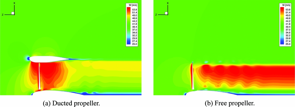
Figure 13. Axial velocity in the vertical symmetry plane of the ducted and free propellers at dash speed.
3.3 Effect of the Duct
To assess the effect of the duct, the performance of the ducted and free propellers were computed using the baseline high-twist blade and the simplified geometry of Figs 4 and 5. The flow was modelled using the RANS equations and the k-ω turbulence model. The Reynolds number was 3.18 × 10⁶ and the tip Mach number was 0.7. Three advance ratios were considered, that is, J = 0, 0.136, 0.540, which correspond to static conditions, cruise speed and dash speed, respectively.
Figures 12(a) and 12(b) show, respectively, the wake visualised using the Q-criterion and the surface pressure coefficient (based on the free-stream velocity) on the ducted high-twist propeller at dash speed. The blade loading shows the importance of the outboard part of the blades with high suction produced near 60% of the blade radius. The complex swirling flow is also well resolved with the current set of CFD grids.
Figures 13(a) and 13(b) compare the flow through the ducted and unducted propellers at the same flight conditions. The differences in the flow-field are substantial and well captured by the simulation. It is clearly shown how the rear part of the duct operates as a diffuser, decreasing the propeller wake speed and increasing the static pressure, so as to induce a positive contribution to the overall thrust.
The predicted performance of the ducted and free propellers are given in Table 1. In static conditions (J = 0), the performance of the ducted propeller is significantly higher than that of the free propeller. For instance, at a low blade pitch angle the ducted propeller gives 24% more thrust with 25% less power. At cruise speed (J = 0.136), the contribution of the duct is still important, and at a medium pitch angle, the ducted propeller gives 10% more thrust with 22% less power.
Table 1 Computed performance of the propulsor

When the speed is higher, the positive effect of the duct reduces due to the increase of the duct drag that compensates the positive contribution of the static pressure in the diffuser. Consider, for example, the flight condition at dash speed (J = 0.54). At fixed blade pitch angle, the thrust and the torque of the ducted propeller are considerably lower, since the acceleration of the flow at the duct inlet reduces the effective angle of attack of the blade. Therefore, to compare the performance at this speed, we alter the angle of attack of the ducted propeller blades to match the thrust of the free propeller. By interpolating results for the ducted and free propellers in Table 1, it is deduced that the torque in the ducted case is only 1% lower than the free propeller value. At this higher advance ratio, the duct is ineffective.
To better understand the role of the duct in the thrust generation, Table 2 reports the force breakdown of the ducted and free propellers at cruise and dash speeds. At cruise speed, the duct contribution is 45% of the overall thrust, and the diffuser effect overcompensates the duct drag force and the reduced effective angle of attack of the propeller blades. At dash speed, the contribution is reduced to 22%, and it is barely sufficient to balance the negative effects. For higher speeds, the duct is detrimental to the propulsor performance.
Table 2 Force breakdown on the ducted and free propellers
3.4 Effect of the blade twist
The propulsor analysed in the previous section is equipped with highly twisted blades. Their twist distribution was designed for the free propeller, and it is therefore interesting to verify if it is also optimal for the ducted configuration. To better understand the effect of the blade twist on the propulsor performance, a new set of blades was considered, having the same sectional shape but a lower twist value (around one-fourth).
The thrust and torque obtained with CFD for the ducted propeller with low-twist blades are given in Table 1. The comparison with the high-twist blade results reveals that the propulsive efficiency of the low-twist blades is lower both at cruise and dash speeds. These results contradict those obtained with the simple panel method(1), and highlight the necessity of using high-fidelity CFD to predict accurately the performance of a ducted propeller. In light of these results, an optimisation of the blade twist distribution was attempted, using a gradient based method coupled to the HMB3 flow solver.
3.5 Optimisation of the twist distribution
The performance of a ducted propeller depends mainly on the blade geometry and on the expansion ratio of the duct. But there are also other factors that might influence the performance, such as
-
(a) the shape of the duct diffuser, which needs to be designed to avoid separations due to the adverse pressure gradient;
-
(b) the shape of the duct inlet lips, whose design determines the behaviour at off-design working conditions such as, for instance, when the flow is not perfectly axial;
-
(c) the clearance between the blade tip and the duct inner surface, which affects the blade-tip losses;
-
(d) the blockage induced by non-aerodynamic parts, such as purely structural component, engine and cooling devices.
This work focuses on the blade and duct geometries. Initially, the twist distribution alone was optimised, and at a second stage, both the blade twist distribution and the duct shape were included in the optimisation process. The results of the twist optimisation are given in this section, while the optimisation including the duct shape follows.
The ducted propeller with the high-twist blades with medium pitch, and with advance ratio corresponding to the LTA cruise speed was considered for the twist optimisation exercise. The baseline performance of the propulsor at these conditions are listed in Table 1, from which we get
 $C_T/C_{T,\text{ref}}=6.861$
and
$C_T/C_{T,\text{ref}}=6.861$
and
 $C_P/C_{P,\text{ref}}=2.206$
. The optimisation objective was to maximise the thrust coefficient CT
, with the power coefficient CP
constrained to the value of the baseline design.
$C_P/C_{P,\text{ref}}=2.206$
. The optimisation objective was to maximise the thrust coefficient CT
, with the power coefficient CP
constrained to the value of the baseline design.
The shape of the duct was fixed, as well as the shape of the blade sections. The only permitted modification to the blade geometry was a perturbation of the initial twist distribution. This perturbation was described by a Bernstein polynomial expansion of order n:
 $$\begin{equation}
\Delta \theta (\xi ) = \sum _{r=0}^{n} \alpha _r K_{r,n} \xi ^r (1-\xi )^{n-r},
\end{equation}$$
$$\begin{equation}
\Delta \theta (\xi ) = \sum _{r=0}^{n} \alpha _r K_{r,n} \xi ^r (1-\xi )^{n-r},
\end{equation}$$
where K r, n is given by
 $$\begin{equation}
K_{r,n} = \left( \begin{array}{c}n \\
r \end{array} \right) = {\displaystyle \frac{n!}{r!(n-r)!}}
\end{equation}$$
$$\begin{equation}
K_{r,n} = \left( \begin{array}{c}n \\
r \end{array} \right) = {\displaystyle \frac{n!}{r!(n-r)!}}
\end{equation}$$
and ξ is the blade span-wise normalised coordinate, which has a value of 0 at the rotation axis and value of 1 at the blade tip.
The gradients of the thrust and power coefficients with respect to the design variables were computed by means of FGMRES-DR(210,70)-GMRES(50). The number of inner iterations was limited to 50, and the CFL number used for computing the pre-conditioning matrix
 $\hat{J}$
, given by Equation (14), was 1,200. The linear solver was run on 128 Intel Xeon E5-2650 2GHz cores, and it took about 12 hours and 1,637 outer iterations to converge the solution of the adjoint equations to a relative residual of 10−7, which is almost half of the time needed to solve the base flow (see Fig. 14). The developed GMRES method proved to be particularly effective for the solution of the adjoint equations that represent a particularly challenging problem in this work, since the derivatives of the two-equation k-ω turbulence model are included. Note also that the base flow is not asymptotically converging but instead enters a limit cycle (see Fig. 14), and this is known to lead to an even tougher linear system for the adjoint variables(Reference Campobasso and Giles8).
$\hat{J}$
, given by Equation (14), was 1,200. The linear solver was run on 128 Intel Xeon E5-2650 2GHz cores, and it took about 12 hours and 1,637 outer iterations to converge the solution of the adjoint equations to a relative residual of 10−7, which is almost half of the time needed to solve the base flow (see Fig. 14). The developed GMRES method proved to be particularly effective for the solution of the adjoint equations that represent a particularly challenging problem in this work, since the derivatives of the two-equation k-ω turbulence model are included. Note also that the base flow is not asymptotically converging but instead enters a limit cycle (see Fig. 14), and this is known to lead to an even tougher linear system for the adjoint variables(Reference Campobasso and Giles8).
Figure 14. Convergence history of the base flow and of the adjoint equations.
Figures 15 and 16 show, respectively, the distribution of the adjoint variable of the thrust and power coefficients relative to the pressure equation for the baseline design. Even if a direct interpretation of the adjoint variable is not easy, by Equation (11) we can infer that modifications to surface regions with higher absolute values of the adjoint variable shall affect more the output functional (CT or CP ). On the other hand, regions with small absolute values of the adjoint variable have negligible influence on the output functional.
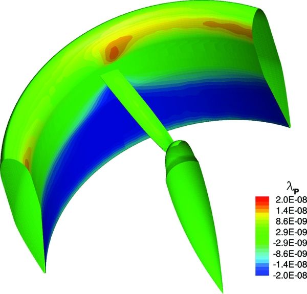
Figure 15. Pressure equation adjoint variable of the thrust coefficient CT .
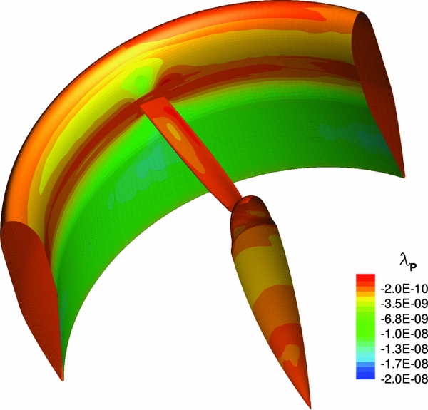
Figure 16. Pressure equation adjoint variable of the power coefficient CP .
Seven coefficients were used for the parametrisation (19), and each coefficient was constrained within the range ( − 5°, 5°). The optimisation loop converged after 15 cycles (see Fig. 17), yielding an increase in the propulsive efficiency of the propulsor of about 1%. This is a moderate improvement over the baseline design and suggests that the original twist distribution was nearly optimal for the ducted propeller configuration. Figure 18 compares the baseline and optimised blade surfaces and shows how the local pitch has been increased next to the blade tip and at the root and decreased in the sections between 65% and 93% of the blade radius. This leads to a higher loading at the tip of the optimised blade, as shown in Figs 19 and 20.
Figure 17. Optimisation history.

Figure 18. Comparison of baseline (light gray) and optimised (dark gray) blade surfaces.
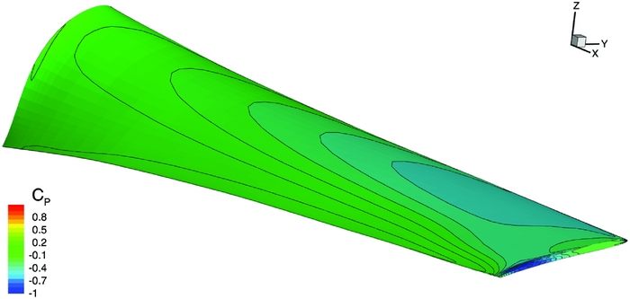
Figure 19. Surface pressure coefficient of the baseline blade (cruise speed, medium blade pitch).
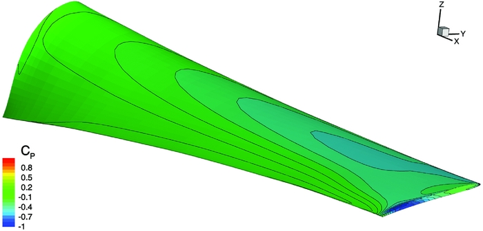
Figure 20. Surface pressure coefficient of the optimised blade (cruise speed, medium blade pitch).
3.6 Optimisation of the duct shape
A further improvement of the propulsor performance is expected if the duct shape and size are included in the optimisation process. As for the twist optimisation case, the optimisation objective was the maximisation of the thrust coefficient CT , with the power coefficient CP constrained to the value of the baseline design.
The blade twist perturbation was described again by the Bernstein polynomial expansion (19). The duct is axisymmetric; therefore, only the section shape needs to be parametrised. The considered design variables allow to vary the shape of the duct diffuser, the radius at the duct outlet and the length of the duct (see Fig. 21). This is done as follows.
-
• The shape of the duct diffuser is described using a Class/Shape Transformation (CST) parametrisation(Reference Kulfan18):
(21)where
$$\begin{equation}
r(\xi _1) = C_{N_1}^{N_2}(\xi _1) \sum _{r=0}^{n} \alpha _r K_{r,n} \xi _1^r (1-\xi _1)^{n-r},
\end{equation}$$
(22)
$$\begin{equation}
C_{N_1}^{N_2}(\xi _1) = \xi _1^{N_1} \left(1-\xi _1^{N_2}\right)
\end{equation}$$
The symbol r represents the radial coordinate of the duct, while ξ1 is a nondimensional variable that ranges from 0 at the duct lip to 1 at the inner flat surface of the duct section, as shown in Fig. 21. To represent the rounded lip at ξ = 0 and the flat surface at ξ = 1, we take N 1 = 0.5 and N 2 = 1.0.
Figure 21. Schematic of the parametrisation of the duct cross-section.
-
• The variation of the duct radius ΔR at the outlet is given by the following two functions:
(23)
$$\begin{equation}
\Delta r(\xi _1) = \Delta R [ 1 - \sin ^2(0.5 \pi \xi _1) ],\\
\end{equation}$$
(24)
$$\begin{equation}
\Delta r(\xi _2) = \Delta R [ 1 - \sin ^2(0.5 \pi \xi _2) ]
\end{equation}$$
The first function is used to parametrise the duct diffuser surface, whereas the second is used for the duct outer surface.
-
• The variation of the duct length ΔL is described by the following function:
where z represents the axial coordinates, positive from the aft to the forward side of the propulsor. The first function is used for the diffuser, while the second is for the outer surface.(25)
$$\begin{equation}
\Delta z(\xi _1) = \Delta L [ 1 - \sin ^2(0.5 \pi \xi _1) ],\\
\end{equation}$$
(26)
$$\begin{equation}
\Delta z(\xi _2) = \Delta L [ 1 - \sin ^2(0.5 \pi \xi _2) ],
\end{equation}$$


Seven coefficients were used for the parametrisation of the twist variation (19). The shape of the duct diffuser was described considering 16 coefficients for the CST parametrisation (22). Two design variables were finally used to define the variation of the duct radius and length in (23) and (25), respectively. There was a total of 25 design variables. The twist coefficients were constrained within the range ( − 5°, 5°). Both the duct radius and length variations were limited to ( − 100mm, 100mm). The optimisation converged after 19 cycles (see Fig. 22), leading to a 2% increase in the propulsive efficiency. Figure 23 shows a comparison of the optimised and baseline surface of the blade and duct. Note that the computed optimal shape of the duct has a larger radius and shorter length. Minor variations have been introduced in the diffuser shape, with the optimised one having a slightly higher curvature near the outflow section.

Figure 22. Optimisation history.

Figure 23. Comparison of baseline (light gray) and optimised (dark gray) blade and duct surfaces.
4.0 CONCLUSIONS
This paper presented the analysis and design of a ducted propeller by means of high-fidelity CFD methods. The numerical results prove the effectiveness of the duct for low-speed operations, where it significantly increased the overall propulsor efficiency. The effect of the blade twist on the performance was also analysed, and results indicate that blades loaded outboard operate with higher efficiency over a wide range of operating conditions. Optimisation of the twist distribution and of the duct shape was then attempted using a quasi-Newton method and an adjoint solver to provide the required gradients. A moderate increase in the propulsor efficiency was obtained using the blade with optimised twist. Further performance improvement was achieved by combined optimisation of the blade twist and the duct shape, which led to a 2% increase in the propulsor efficiency. The above optimisations were facilitated by the developed nested Krylov-subspace method for solving the adjoint equations.
ACKNOWLEDGEMENTS
The research leading to these results has received funding from the LOCATE project of Hybrid Air Vehicles Ltd and Innovate UK, grant agreement no. 101798. Results were obtained using the EPSRC funded ARCHIE-WeSt High Performance Computer (www.archie-west.ac.uk), EPSRC grant no. EP/K000586/1.