


1 Introduction
We study the behaviour of thermodynamic fluctuations in compressible aerodynamic turbulence. It is well known (Hansen Reference Hansen1958, figure 1, p. 57) that, for temperatures
 $T\lessapprox 2000~\text{K}$
, the equation of state of air flow can be reasonably approximated by the so-called perfect-gas equation of state (Liepmann & Roshko Reference Liepmann and Roshko1957, § 1, pp. 1–37)
$T\lessapprox 2000~\text{K}$
, the equation of state of air flow can be reasonably approximated by the so-called perfect-gas equation of state (Liepmann & Roshko Reference Liepmann and Roshko1957, § 1, pp. 1–37)
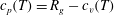
 $$\begin{eqnarray}\displaystyle {\mathcal{Z}}(\unicode[STIX]{x1D70C},T):={\displaystyle \frac{p}{\unicode[STIX]{x1D70C}R_{g}T}}=1\;\Longleftrightarrow \;p=\unicode[STIX]{x1D70C}R_{g}T\;\Longrightarrow \;\left\{\begin{array}{@{}l@{}}a=\sqrt{\unicode[STIX]{x1D6FE}(T)\,R_{g}T}\\ \unicode[STIX]{x1D6FE}(T):={\displaystyle \frac{c_{p}(T)}{c_{v}(T)}}={\displaystyle \frac{c_{p}(T)}{c_{p}(T)-R_{g}}},\end{array}\right. & & \displaystyle\end{eqnarray}$$
where
 $R_{g}=\text{const.}$
is the gas constant (
$R_{g}=\text{const.}$
is the gas constant (
 $R_{g}=287.04~\text{m}^{2}~\text{s}^{-2}\,\text{ K}^{-1}$
for air),
$R_{g}=287.04~\text{m}^{2}~\text{s}^{-2}\,\text{ K}^{-1}$
for air),
 $p$
is the pressure,
$p$
is the pressure,
 $\unicode[STIX]{x1D70C}$
is the density,
$\unicode[STIX]{x1D70C}$
is the density,
 $T$
is the temperature,
$T$
is the temperature,
 ${\mathcal{Z}}$
is the compressibility factor (Hansen Reference Hansen1958, p. 7),
${\mathcal{Z}}$
is the compressibility factor (Hansen Reference Hansen1958, p. 7),
 $c_{p}(T)$
and
$c_{p}(T)$
and
 $c_{v}(T)=c_{p}(T)-R_{g}$
are the specific heats at constant pressure or volume, with ratio
$c_{v}(T)=c_{p}(T)-R_{g}$
are the specific heats at constant pressure or volume, with ratio
 $\unicode[STIX]{x1D6FE}(T)$
, and
$\unicode[STIX]{x1D6FE}(T)$
, and
 $a(T)$
is the sound speed. At higher temperatures, dissociation of oxygen is the first phenomenon causing departure from (1.1), this departure occurring at higher temperatures with increasing pressure (Hansen Reference Hansen1958, figure 1, p. 57). Throughout the paper, the validity of (1.1) is assumed, and its implications for thermodynamic fluctuations in compressible turbulent flows are studied.
$a(T)$
is the sound speed. At higher temperatures, dissociation of oxygen is the first phenomenon causing departure from (1.1), this departure occurring at higher temperatures with increasing pressure (Hansen Reference Hansen1958, figure 1, p. 57). Throughout the paper, the validity of (1.1) is assumed, and its implications for thermodynamic fluctuations in compressible turbulent flows are studied.
Standard decomposition
 $(\cdot )=\overline{(\cdot )}+(\cdot )^{\prime }$
(Huang, Coleman & Bradshaw Reference Huang, Coleman and Bradshaw1995, (2.1), p. 188) in Reynolds (ensemble) averages
$(\cdot )=\overline{(\cdot )}+(\cdot )^{\prime }$
(Huang, Coleman & Bradshaw Reference Huang, Coleman and Bradshaw1995, (2.1), p. 188) in Reynolds (ensemble) averages
 $\overline{(\cdot )}$
and fluctuations
$\overline{(\cdot )}$
and fluctuations
 $(\cdot )^{\prime }$
is used in the paper, for any flow quantity
$(\cdot )^{\prime }$
is used in the paper, for any flow quantity
 $(\cdot )$
. An initial attempt to use Favre (mass-weighted) decomposition,
$(\cdot )$
. An initial attempt to use Favre (mass-weighted) decomposition,
 $(\cdot )=\widetilde{(\cdot )}+(\cdot )^{\prime \prime }$
, for
$(\cdot )=\widetilde{(\cdot )}+(\cdot )^{\prime \prime }$
, for
 $T$
and
$T$
and
 $s$
, as is generally the case for transport equations (Gerolymos & Vallet Reference Gerolymos and Vallet2014), was inconclusive, both because it did not offer any particular conciseness in the relations between thermodynamic fluctuations and because it presents some mathematical difficulties in defining coefficients of variation and correlation coefficients in a strict mathematical sense. Furthermore, the correlation coefficient
$s$
, as is generally the case for transport equations (Gerolymos & Vallet Reference Gerolymos and Vallet2014), was inconclusive, both because it did not offer any particular conciseness in the relations between thermodynamic fluctuations and because it presents some mathematical difficulties in defining coefficients of variation and correlation coefficients in a strict mathematical sense. Furthermore, the correlation coefficient
 $c_{\unicode[STIX]{x1D70C}^{\prime }T^{\prime }}$
comes out as an important parameter in the present work, independently of the relative importance of
$c_{\unicode[STIX]{x1D70C}^{\prime }T^{\prime }}$
comes out as an important parameter in the present work, independently of the relative importance of
 $\overline{T^{\prime \prime }}=-c_{\unicode[STIX]{x1D70C}^{\prime }T^{\prime }}\,\text{CV}_{\unicode[STIX]{x1D70C}^{\prime }}\,\text{CV}_{T^{\prime }}\,\bar{T}$
.
$\overline{T^{\prime \prime }}=-c_{\unicode[STIX]{x1D70C}^{\prime }T^{\prime }}\,\text{CV}_{\unicode[STIX]{x1D70C}^{\prime }}\,\text{CV}_{T^{\prime }}\,\bar{T}$
.
The intensity of the fluctuations of thermodynamic state variables (
 $p$
,
$p$
,
 $\unicode[STIX]{x1D70C}$
,
$\unicode[STIX]{x1D70C}$
,
 $T$
) is quantified by their coefficients of variation (
$T$
) is quantified by their coefficients of variation (
 $\text{CV}_{\unicode[STIX]{x1D70C}^{\prime }}:=\bar{\unicode[STIX]{x1D70C}}^{-1}\unicode[STIX]{x1D70C}_{rms}^{\prime }$
,
$\text{CV}_{\unicode[STIX]{x1D70C}^{\prime }}:=\bar{\unicode[STIX]{x1D70C}}^{-1}\unicode[STIX]{x1D70C}_{rms}^{\prime }$
,
 $\text{CV}_{T^{\prime }}:=\bar{T}^{-1}T_{rms}^{\prime }$
,
$\text{CV}_{T^{\prime }}:=\bar{T}^{-1}T_{rms}^{\prime }$
,
 $\text{CV}_{p^{\prime }}:=\bar{p}^{-1}p_{rms}^{\prime }$
) i.e. their relative r.m.s. (root-mean-square) fluctuation levels (§ 2.1). The perfect-gas equation of state (1.1) implies exact nonlinear relations between coefficients of variation of the state variables and correlation coefficients between thermodynamic fluctuations. Such relations are of general validity, independently of the particular flow that is investigated. Thermodynamic relations based on the linearized truncation
$\text{CV}_{p^{\prime }}:=\bar{p}^{-1}p_{rms}^{\prime }$
) i.e. their relative r.m.s. (root-mean-square) fluctuation levels (§ 2.1). The perfect-gas equation of state (1.1) implies exact nonlinear relations between coefficients of variation of the state variables and correlation coefficients between thermodynamic fluctuations. Such relations are of general validity, independently of the particular flow that is investigated. Thermodynamic relations based on the linearized truncation
 $\bar{p}^{-1}\,p^{\prime }\approxeq \bar{\unicode[STIX]{x1D70C}}^{-1}\,\unicode[STIX]{x1D70C}^{\prime }+\bar{T}^{-1}\,T^{\prime }$
(Gatski & Bonnet Reference Gatski and Bonnet2009, (3.114), p. 72) of the exact expansion of (1.1) are widely used (Kovásznay Reference Kovásznay1953; Taulbee & VanOsdol Reference Taulbee and Van Osdol1991): this approach studies compressible turbulence in the limiting case of small relative fluctuation amplitudes, neglecting quadratic or higher-order terms. The point should be made, nonetheless, that the assumption that the relative
$\bar{p}^{-1}\,p^{\prime }\approxeq \bar{\unicode[STIX]{x1D70C}}^{-1}\,\unicode[STIX]{x1D70C}^{\prime }+\bar{T}^{-1}\,T^{\prime }$
(Gatski & Bonnet Reference Gatski and Bonnet2009, (3.114), p. 72) of the exact expansion of (1.1) are widely used (Kovásznay Reference Kovásznay1953; Taulbee & VanOsdol Reference Taulbee and Van Osdol1991): this approach studies compressible turbulence in the limiting case of small relative fluctuation amplitudes, neglecting quadratic or higher-order terms. The point should be made, nonetheless, that the assumption that the relative
 $\text{r.m.s.}$
-levels,
$\text{r.m.s.}$
-levels,
 $\bar{\unicode[STIX]{x1D70C}}^{-1}\unicode[STIX]{x1D70C}_{rms}^{\prime }$
and
$\bar{\unicode[STIX]{x1D70C}}^{-1}\unicode[STIX]{x1D70C}_{rms}^{\prime }$
and
 $\bar{T}^{-1}T_{rms}^{\prime }$
, are small, which is used in some parts of the paper, is less stringent than assuming that the instantaneous levels,
$\bar{T}^{-1}T_{rms}^{\prime }$
, are small, which is used in some parts of the paper, is less stringent than assuming that the instantaneous levels,
 $\bar{\unicode[STIX]{x1D70C}}^{-1}\unicode[STIX]{x1D70C}^{\prime }$
and
$\bar{\unicode[STIX]{x1D70C}}^{-1}\unicode[STIX]{x1D70C}^{\prime }$
and
 $\bar{T}^{-1}T^{\prime }$
are invariably small, as in the standard linearized approximation (Gatski & Bonnet Reference Gatski and Bonnet2009, (3.114), p. 72). Mahesh, Lele & Moin (Reference Mahesh, Lele and Moin1997) use, in the context of the Reynolds analogy assumptions (Morkovin Reference Morkovin and Favre1962), the term ‘weak form’ for relations in a
$\bar{T}^{-1}T^{\prime }$
are invariably small, as in the standard linearized approximation (Gatski & Bonnet Reference Gatski and Bonnet2009, (3.114), p. 72). Mahesh, Lele & Moin (Reference Mahesh, Lele and Moin1997) use, in the context of the Reynolds analogy assumptions (Morkovin Reference Morkovin and Favre1962), the term ‘weak form’ for relations in a
 $\text{r.m.s.}$
sense, as opposed to ‘strong form’ for instantaneous relations. This point is further is highlighted in Barre & Bonnet (Reference Barre and Bonnet2015) who distinguish between the SRA (strong Reynolds analogy) involving relations between variances and covariances and the VSRA (very strong Reynolds analogy) invoking instantaneous fluctuating relations. The acoustic, vorticity and entropy modes describing the essential dynamics of compressible turbulence (Kovásznay Reference Kovásznay1953) are the mathematical result of linearized analysis. However, the higher-order (nonlinear) coupling between modes identified from the general small-perturbation series expansion of the compressible Navier–Stokes equations (Chu & Kovásznay Reference Chu and Kovásznay1958) is essential in completing this now classic view of gas dynamic turbulence. Nonetheless, Blaisdell, Mansour & Reynolds (Reference Blaisdell, Mansour and Reynolds1993) point out the difficulty of using this approach ‘to study fully nonlinear turbulence for which the decomposition into such modes cannot be made’.
$\text{r.m.s.}$
sense, as opposed to ‘strong form’ for instantaneous relations. This point is further is highlighted in Barre & Bonnet (Reference Barre and Bonnet2015) who distinguish between the SRA (strong Reynolds analogy) involving relations between variances and covariances and the VSRA (very strong Reynolds analogy) invoking instantaneous fluctuating relations. The acoustic, vorticity and entropy modes describing the essential dynamics of compressible turbulence (Kovásznay Reference Kovásznay1953) are the mathematical result of linearized analysis. However, the higher-order (nonlinear) coupling between modes identified from the general small-perturbation series expansion of the compressible Navier–Stokes equations (Chu & Kovásznay Reference Chu and Kovásznay1958) is essential in completing this now classic view of gas dynamic turbulence. Nonetheless, Blaisdell, Mansour & Reynolds (Reference Blaisdell, Mansour and Reynolds1993) point out the difficulty of using this approach ‘to study fully nonlinear turbulence for which the decomposition into such modes cannot be made’.
Often, in studies of compressible turbulence, some representative Mach number is assumed to quantify compressibility effects (Smits & Dussauge Reference Smits and Dussauge2006, § 4.5, pp. 105–108), e.g. the turbulent Mach number
 $M_{T}$
(Gatski & Bonnet Reference Gatski and Bonnet2009, (5.1), p. 118), which is essentially (Blaisdell et al.
Reference Blaisdell, Mansour and Reynolds1993, p. 454) approximately equal to
$M_{T}$
(Gatski & Bonnet Reference Gatski and Bonnet2009, (5.1), p. 118), which is essentially (Blaisdell et al.
Reference Blaisdell, Mansour and Reynolds1993, p. 454) approximately equal to
 $M_{rms}^{\prime }$
(provided
$M_{rms}^{\prime }$
(provided
 $\text{CV}_{T^{\prime }}$
is sufficiently small), or the gradient Mach number
$\text{CV}_{T^{\prime }}$
is sufficiently small), or the gradient Mach number
 $M_{g}$
(Smits & Dussauge Reference Smits and Dussauge2006, p. 107), introduced by Sarkar (Reference Sarkar1995). The widespread use of such scalings should be attributed to the deliberate choice of attempting to relate compressibility effects on turbulence to parameters of the dynamic (velocity
$M_{g}$
(Smits & Dussauge Reference Smits and Dussauge2006, p. 107), introduced by Sarkar (Reference Sarkar1995). The widespread use of such scalings should be attributed to the deliberate choice of attempting to relate compressibility effects on turbulence to parameters of the dynamic (velocity
 $\bar{u}_{i}+u_{i}^{\prime }$
) field. Correlations based on these local turbulence-representative Mach numbers lack universality, in the sense that their applicability is flow dependent. On the contrary, Morkovin’s (Reference Morkovin and Favre1962) ideas on the effects of compressibility on turbulence, directly point to
$\bar{u}_{i}+u_{i}^{\prime }$
) field. Correlations based on these local turbulence-representative Mach numbers lack universality, in the sense that their applicability is flow dependent. On the contrary, Morkovin’s (Reference Morkovin and Favre1962) ideas on the effects of compressibility on turbulence, directly point to
 $\text{CV}_{\unicode[STIX]{x1D70C}^{\prime }}$
as the primary indicator, a fact explicitly formulated by Bradshaw (Reference Bradshaw1977).
$\text{CV}_{\unicode[STIX]{x1D70C}^{\prime }}$
as the primary indicator, a fact explicitly formulated by Bradshaw (Reference Bradshaw1977).
The idea that thermodynamic turbulence i.e.
 $\{p^{\prime },\unicode[STIX]{x1D70C}^{\prime },T^{\prime },s^{\prime }\}$
is subordinate to the dynamic field
$\{p^{\prime },\unicode[STIX]{x1D70C}^{\prime },T^{\prime },s^{\prime }\}$
is subordinate to the dynamic field
 $\{\bar{u}_{i},u_{i}^{\prime }\}$
is central in compressible-turbulence research. There are numerous examples of this approach, e.g. various parametrizations in terms of
$\{\bar{u}_{i},u_{i}^{\prime }\}$
is central in compressible-turbulence research. There are numerous examples of this approach, e.g. various parametrizations in terms of
 $M_{T}$
(Donzis & Jagannathan Reference Donzis and Jagannathan2013) or
$M_{T}$
(Donzis & Jagannathan Reference Donzis and Jagannathan2013) or
 $M_{g}$
(Sarkar Reference Sarkar1995), but also the various forms of Reynolds analogy (Huang et al.
Reference Huang, Coleman and Bradshaw1995; Guarini et al.
Reference Guarini, Moser, Shariff and Wray2000; Zhang et al.
Reference Zhang, Bi, Hussain and She2013) relating shear-flow temperature transport
$M_{g}$
(Sarkar Reference Sarkar1995), but also the various forms of Reynolds analogy (Huang et al.
Reference Huang, Coleman and Bradshaw1995; Guarini et al.
Reference Guarini, Moser, Shariff and Wray2000; Zhang et al.
Reference Zhang, Bi, Hussain and She2013) relating shear-flow temperature transport
 $\overline{T^{\prime }v^{\prime }}$
to momentum transport
$\overline{T^{\prime }v^{\prime }}$
to momentum transport
 $\overline{u^{\prime }v^{\prime }}$
. The underlying assumption of all these approaches is that
$\overline{u^{\prime }v^{\prime }}$
. The underlying assumption of all these approaches is that
 $p^{\prime }$
is essentially a consequence of the velocity field
$p^{\prime }$
is essentially a consequence of the velocity field
 $\{\bar{u}_{i},u_{i}^{\prime }\}$
, through the compressible-flow Poisson equation (Gerolymos, Sénéchal & Vallet Reference Gerolymos, Sénéchal and Vallet2013, (A 1e), p. 46). To leading order in
$\{\bar{u}_{i},u_{i}^{\prime }\}$
, through the compressible-flow Poisson equation (Gerolymos, Sénéchal & Vallet Reference Gerolymos, Sénéchal and Vallet2013, (A 1e), p. 46). To leading order in
 $\text{CV}_{\unicode[STIX]{x1D70C}^{\prime }}$
(Foysi, Sarkar & Friedrich Reference Foysi, Sarkar and Friedrich2004), the source terms of this Poisson equation are the basic incompressible mechanisms (Kim Reference Kim1989, slow, rapid and Stokes), with variable
$\text{CV}_{\unicode[STIX]{x1D70C}^{\prime }}$
(Foysi, Sarkar & Friedrich Reference Foysi, Sarkar and Friedrich2004), the source terms of this Poisson equation are the basic incompressible mechanisms (Kim Reference Kim1989, slow, rapid and Stokes), with variable
 $\bar{\unicode[STIX]{x1D70C}}$
and
$\bar{\unicode[STIX]{x1D70C}}$
and
 $\bar{T}$
to account for mean-flow stratification, in the sense of Morkovin’s (Reference Morkovin and Favre1962) hypothesis. Beyond this regime, when
$\bar{T}$
to account for mean-flow stratification, in the sense of Morkovin’s (Reference Morkovin and Favre1962) hypothesis. Beyond this regime, when
 $\text{CV}_{\unicode[STIX]{x1D70C}^{\prime }}$
is high, several other source terms in the Poisson equation for
$\text{CV}_{\unicode[STIX]{x1D70C}^{\prime }}$
is high, several other source terms in the Poisson equation for
 $p^{\prime }$
, representing compressible-turbulence (
$p^{\prime }$
, representing compressible-turbulence (
 $\unicode[STIX]{x1D70C}^{\prime }$
) mechanisms may become important (Foysi et al.
Reference Foysi, Sarkar and Friedrich2004), including the wave-like term (Pantano & Sarkar Reference Pantano and Sarkar2002): coupling between
$\unicode[STIX]{x1D70C}^{\prime }$
) mechanisms may become important (Foysi et al.
Reference Foysi, Sarkar and Friedrich2004), including the wave-like term (Pantano & Sarkar Reference Pantano and Sarkar2002): coupling between
 $p^{\prime }$
and
$p^{\prime }$
and
 $\unicode[STIX]{x1D70C}^{\prime }$
becomes important. Notice also, that the
$\unicode[STIX]{x1D70C}^{\prime }$
becomes important. Notice also, that the
 $p^{\prime }$
-Hessian is governed, in compressible flow, by a specific transport equation (Suman & Girimaji Reference Suman and Girimaji2001, (2.9), p. 292), involving
$p^{\prime }$
-Hessian is governed, in compressible flow, by a specific transport equation (Suman & Girimaji Reference Suman and Girimaji2001, (2.9), p. 292), involving
 $\unicode[STIX]{x1D70C}^{\prime }$
-dependent terms.
$\unicode[STIX]{x1D70C}^{\prime }$
-dependent terms.
The particular approach of compressible-turbulence analysis notwithstanding, thermodynamic fluctuations are interrelated by the equation of state (1.1) and its basic thermodynamic (Liepmann & Roshko Reference Liepmann and Roshko1957, § 1, pp. 1–37) consequences (1.1). There are, however, few studies concentrating on these relations. Donzis & Jagannathan (Reference Donzis and Jagannathan2013) have investigated in detail the behaviour of thermodynamic fluctuations
 $\{p^{\prime },\unicode[STIX]{x1D70C}^{\prime },T^{\prime }\}$
in sustained compressible homogenous isotropic turbulence (HIT), including the
$\{p^{\prime },\unicode[STIX]{x1D70C}^{\prime },T^{\prime }\}$
in sustained compressible homogenous isotropic turbulence (HIT), including the
 $c_{\unicode[STIX]{x1D70C}^{\prime }T^{\prime }}$
correlation coefficient, skewness, flatness and p.d.f.s (probability density functions). This study (Donzis & Jagannathan Reference Donzis and Jagannathan2013) highlights the influence of compressibility
$c_{\unicode[STIX]{x1D70C}^{\prime }T^{\prime }}$
correlation coefficient, skewness, flatness and p.d.f.s (probability density functions). This study (Donzis & Jagannathan Reference Donzis and Jagannathan2013) highlights the influence of compressibility
 $\text{CV}_{\unicode[STIX]{x1D70C}^{\prime }}$
, p.d.f.s tending to near-Gaussian values for skewness and flatness with increasing
$\text{CV}_{\unicode[STIX]{x1D70C}^{\prime }}$
, p.d.f.s tending to near-Gaussian values for skewness and flatness with increasing
 $M_{T}$
implying increasing
$M_{T}$
implying increasing
 $\text{CV}_{\unicode[STIX]{x1D70C}^{\prime }}$
. Gerolymos & Vallet (Reference Gerolymos and Vallet2014) have studied, for compressible plane channel flow, the budgets of the transport equations for the variances and fluxes of the thermodynamic fluctuations
$\text{CV}_{\unicode[STIX]{x1D70C}^{\prime }}$
. Gerolymos & Vallet (Reference Gerolymos and Vallet2014) have studied, for compressible plane channel flow, the budgets of the transport equations for the variances and fluxes of the thermodynamic fluctuations
 $\{p^{\prime },\unicode[STIX]{x1D70C}^{\prime },T^{\prime },s^{\prime }\}$
, and provided data for correlation coefficients between thermodynamic fluctuations (Gerolymos & Vallet Reference Gerolymos and Vallet2014, figure 7, p. 723). Wei & Pollard (Reference Wei and Pollard2011, figure 1, p. 6) suggest that the correlation coefficient
$\{p^{\prime },\unicode[STIX]{x1D70C}^{\prime },T^{\prime },s^{\prime }\}$
, and provided data for correlation coefficients between thermodynamic fluctuations (Gerolymos & Vallet Reference Gerolymos and Vallet2014, figure 7, p. 723). Wei & Pollard (Reference Wei and Pollard2011, figure 1, p. 6) suggest that the correlation coefficient
 $c_{p^{\prime }\unicode[STIX]{x1D70C}^{\prime }}$
decreases near the wall with increasing Mach number, but its level is probably also
$c_{p^{\prime }\unicode[STIX]{x1D70C}^{\prime }}$
decreases near the wall with increasing Mach number, but its level is probably also
 $Re$
-dependent (Gerolymos & Vallet Reference Gerolymos and Vallet2014). Several authors (Lechner, Sesterhenn & Friedrich Reference Lechner, Sesterhenn and Friedrich2001; Shadloo, Hadjadj & Hussain Reference Shadloo, Hadjadj and Hussain2015) have used two-dimensional (2-D) scatter plots of relative amplitudes to gain insight into the correlation between thermodynamic fluctuations. Duan, Choudhari & Zhang (Reference Duan, Choudhari and Zhang2016) studied using direct numerical simulation (DNS) 2-point/2-time
$Re$
-dependent (Gerolymos & Vallet Reference Gerolymos and Vallet2014). Several authors (Lechner, Sesterhenn & Friedrich Reference Lechner, Sesterhenn and Friedrich2001; Shadloo, Hadjadj & Hussain Reference Shadloo, Hadjadj and Hussain2015) have used two-dimensional (2-D) scatter plots of relative amplitudes to gain insight into the correlation between thermodynamic fluctuations. Duan, Choudhari & Zhang (Reference Duan, Choudhari and Zhang2016) studied using direct numerical simulation (DNS) 2-point/2-time
 $p^{\prime }$
-correlations in a hypersonic
$p^{\prime }$
-correlations in a hypersonic
 $\bar{M}_{e}\approxeq 5.86$
cold-wall boundary layer and obtained detailed information on the convective velocity of
$\bar{M}_{e}\approxeq 5.86$
cold-wall boundary layer and obtained detailed information on the convective velocity of
 $p^{\prime }$
in the boundary layer and on the acoustic field radiated in the free stream.
$p^{\prime }$
in the boundary layer and on the acoustic field radiated in the free stream.
In the absence of direct
 $p^{\prime }$
measurements, early shear-flow hot-wire practice (Kovásznay Reference Kovásznay1953; Kistler Reference Kistler1959; Morkovin Reference Morkovin and Favre1962), assumed that in supersonic (
$p^{\prime }$
measurements, early shear-flow hot-wire practice (Kovásznay Reference Kovásznay1953; Kistler Reference Kistler1959; Morkovin Reference Morkovin and Favre1962), assumed that in supersonic (
 $\bar{M}_{e}\lessapprox 5$
) boundary layers
$\bar{M}_{e}\lessapprox 5$
) boundary layers
 $\text{CV}_{p^{\prime }}\ll \text{CV}_{\unicode[STIX]{x1D70C}^{\prime }}=O(\text{CV}_{T^{\prime }})$
, expecting (Morkovin Reference Morkovin and Favre1962) that
$\text{CV}_{p^{\prime }}\ll \text{CV}_{\unicode[STIX]{x1D70C}^{\prime }}=O(\text{CV}_{T^{\prime }})$
, expecting (Morkovin Reference Morkovin and Favre1962) that
 $\text{CV}_{p^{\prime }}$
would become important only at higher external flow Mach number
$\text{CV}_{p^{\prime }}$
would become important only at higher external flow Mach number
 $\bar{M}_{e}$
. Of course DNS data (Coleman, Kim & Moser Reference Coleman, Kim and Moser1995) largely moderate this assumption, since near the wall, although
$\bar{M}_{e}$
. Of course DNS data (Coleman, Kim & Moser Reference Coleman, Kim and Moser1995) largely moderate this assumption, since near the wall, although
 $\text{CV}_{p^{\prime }}<\text{CV}_{\unicode[STIX]{x1D70C}^{\prime }}$
, they both are still of the same order of magnitude (Gerolymos & Vallet Reference Gerolymos and Vallet2014), while further away from the wall (wake region)
$\text{CV}_{p^{\prime }}<\text{CV}_{\unicode[STIX]{x1D70C}^{\prime }}$
, they both are still of the same order of magnitude (Gerolymos & Vallet Reference Gerolymos and Vallet2014), while further away from the wall (wake region)
 $\text{CV}_{p^{\prime }}>\text{CV}_{\unicode[STIX]{x1D70C}^{\prime }}$
. Laderman & Demetriades (Reference Laderman and Demetriades1974) were probably the first to make an approximate assessment of
$\text{CV}_{p^{\prime }}>\text{CV}_{\unicode[STIX]{x1D70C}^{\prime }}$
. Laderman & Demetriades (Reference Laderman and Demetriades1974) were probably the first to make an approximate assessment of
 $\text{CV}_{p^{\prime }}$
in their analysis of
$\text{CV}_{p^{\prime }}$
in their analysis of
 $\bar{M}_{e}\approxeq 9.4$
boundary-layer measurements: interestingly they assumed that
$\bar{M}_{e}\approxeq 9.4$
boundary-layer measurements: interestingly they assumed that
 $p^{\prime }$
and
$p^{\prime }$
and
 $s^{\prime }$
were uncorrelated (Laderman & Demetriades Reference Laderman and Demetriades1974,
$s^{\prime }$
were uncorrelated (Laderman & Demetriades Reference Laderman and Demetriades1974,
 $c_{s^{\prime }p^{\prime }}=0$
; table 2, p. 138). This assumption is approximately verified by recent wall turbulence DNS data (Gerolymos & Vallet Reference Gerolymos and Vallet2014, figure 7, p. 723). Barre & Bonnet (Reference Barre and Bonnet2015), citing Blaisdell et al. (Reference Blaisdell, Mansour and Reynolds1993), associate the approximation
$c_{s^{\prime }p^{\prime }}=0$
; table 2, p. 138). This assumption is approximately verified by recent wall turbulence DNS data (Gerolymos & Vallet Reference Gerolymos and Vallet2014, figure 7, p. 723). Barre & Bonnet (Reference Barre and Bonnet2015), citing Blaisdell et al. (Reference Blaisdell, Mansour and Reynolds1993), associate the approximation
 $c_{s^{\prime }p^{\prime }}=0$
with the decoupling of acoustic and entropy modes in supersonic turbulence (Kovásznay Reference Kovásznay1953). On the other hand, Pantano & Sarkar (Reference Pantano and Sarkar2002, pp. 351–352) using the thermodynamic identity
$c_{s^{\prime }p^{\prime }}=0$
with the decoupling of acoustic and entropy modes in supersonic turbulence (Kovásznay Reference Kovásznay1953). On the other hand, Pantano & Sarkar (Reference Pantano and Sarkar2002, pp. 351–352) using the thermodynamic identity
 $D_{t}p=(\unicode[STIX]{x2202}_{\unicode[STIX]{x1D70C}}p)_{s}\,D_{t}\unicode[STIX]{x1D70C}+(\unicode[STIX]{x2202}_{s}p)_{\unicode[STIX]{x1D70C}}\,D_{t}s$
assumed that
$D_{t}p=(\unicode[STIX]{x2202}_{\unicode[STIX]{x1D70C}}p)_{s}\,D_{t}\unicode[STIX]{x1D70C}+(\unicode[STIX]{x2202}_{s}p)_{\unicode[STIX]{x1D70C}}\,D_{t}s$
assumed that
 $ps$
-coupling becomes dominant as the convective Mach number
$ps$
-coupling becomes dominant as the convective Mach number
 $M_{c}$
increases.
$M_{c}$
increases.
Contrary to studies of astrophysical turbulence, where a tentative thermodynamic model is constructed assuming explicitly isothermal or polytropic behaviour (Banerjee & Galtier Reference Banerjee and Galtier2014), in aerodynamic (more generally gas dynamic) flows the working medium thermodynamics is known, and the weakly compressible regime or the quasi-incompressible limit are the consequences of the characteristic flow Mach number
 $M_{ref}\rightarrow 0$
. In modelling work, Rubesin (Reference Rubesin1976, (47), p.10) introduces the assumption of polytropic behaviour of thermodynamic fluctuations, with polytropic exponent
$M_{ref}\rightarrow 0$
. In modelling work, Rubesin (Reference Rubesin1976, (47), p.10) introduces the assumption of polytropic behaviour of thermodynamic fluctuations, with polytropic exponent
 $n_{P}$
which can be considered a modelling parameter (flow dependent). This polytropic behaviour can also be considered in an
$n_{P}$
which can be considered a modelling parameter (flow dependent). This polytropic behaviour can also be considered in an
 $\text{r.m.s.}$
-sense (Barre & Bonnet Reference Barre and Bonnet2015). Notice that analysis of plane-mixing-layer DNS data at convective Mach number
$\text{r.m.s.}$
-sense (Barre & Bonnet Reference Barre and Bonnet2015). Notice that analysis of plane-mixing-layer DNS data at convective Mach number
 $M_{c}=1$
clearly indicate that free shear turbulence is not polytropic (Barre & Bonnet Reference Barre and Bonnet2015, figure 13, p. 331).
$M_{c}=1$
clearly indicate that free shear turbulence is not polytropic (Barre & Bonnet Reference Barre and Bonnet2015, figure 13, p. 331).
The above cited references explicitly study thermodynamic fluctuations and their correlations. We do not include here many other studies on the dynamic field in compressible turbulence, which are reviewed elsewhere (Lele Reference Lele1994; Guarini et al. Reference Guarini, Moser, Shariff and Wray2000; Duan & Martín Reference Duan and Martín2011; Lagha et al. Reference Lagha, Kim, Eldredge and Zhong2011; Zhang et al. Reference Zhang, Bi, Hussain and She2013; Gerolymos & Vallet Reference Gerolymos and Vallet2014; Modesti & Pirozzoli Reference Modesti and Pirozzoli2016). Phenomenological models such as eddy-shocklets (Lee, Lele & Moin Reference Lee, Lele and Moin1991), pseudo-sound (Ristorcelli Reference Ristorcelli1997) and compressibility damping of the velocity/pressure-gradient correlation (Sarkar Reference Sarkar1995; Pantano & Sarkar Reference Pantano and Sarkar2002) have evolved to explain the effects of compressibility on turbulence dynamics.
The paper focuses on the relations between thermodynamic fluctuations
 $\{p^{\prime },\unicode[STIX]{x1D70C}^{\prime },T^{\prime },s^{\prime }\}$
implied by (1.1). Compressibility
$\{p^{\prime },\unicode[STIX]{x1D70C}^{\prime },T^{\prime },s^{\prime }\}$
implied by (1.1). Compressibility
 $\text{CV}_{\unicode[STIX]{x1D70C}^{\prime }}$
principally controls the level of thermodynamic fluctuations
$\text{CV}_{\unicode[STIX]{x1D70C}^{\prime }}$
principally controls the level of thermodynamic fluctuations
 $\{\text{CV}_{p^{\prime }},\text{CV}_{\unicode[STIX]{x1D70C}^{\prime }},\text{CV}_{T^{\prime }}\}$
. On the other hand, the set of ratios of these relative levels, along with all possible 2-moment correlation coefficients
$\{\text{CV}_{p^{\prime }},\text{CV}_{\unicode[STIX]{x1D70C}^{\prime }},\text{CV}_{T^{\prime }}\}$
. On the other hand, the set of ratios of these relative levels, along with all possible 2-moment correlation coefficients
 $$\begin{eqnarray}\displaystyle \text{TTS}:=\left\{{\displaystyle \frac{\text{CV}_{T^{\prime }}}{\text{CV}_{\unicode[STIX]{x1D70C}^{\prime }}}},{\displaystyle \frac{\text{CV}_{p^{\prime }}}{\text{CV}_{\unicode[STIX]{x1D70C}^{\prime }}}},{\displaystyle \frac{s_{rms}^{\prime }}{R_{g}\,\text{CV}_{\unicode[STIX]{x1D70C}^{\prime }}}},c_{\unicode[STIX]{x1D70C}^{\prime }T^{\prime }},c_{p^{\prime }\unicode[STIX]{x1D70C}^{\prime }},c_{p^{\prime }T^{\prime }},c_{s^{\prime }\unicode[STIX]{x1D70C}^{\prime }},c_{s^{\prime }T^{\prime }},c_{s^{\prime }p^{\prime }}\right\} & & \displaystyle\end{eqnarray}$$
defines, in the sense of Bradshaw (Reference Bradshaw1977), the thermodynamic turbulence structure of the flow. The analysis of DNS data will show that, although weakly (slowly) dependent on the characteristic Mach number of the flow, the set TTS (1.2) is rather the footprint of the specific type of flow. Furthermore, for weakly compressible turbulence (
 $\text{CV}_{\unicode[STIX]{x1D70C}^{\prime }}\ll 1$
) the knowledge of any couple of elements of TTS suffices to determine to
$\text{CV}_{\unicode[STIX]{x1D70C}^{\prime }}\ll 1$
) the knowledge of any couple of elements of TTS suffices to determine to
 $O(\text{CV}_{\unicode[STIX]{x1D70C}^{\prime }})$
all the other elements. We use the
$O(\text{CV}_{\unicode[STIX]{x1D70C}^{\prime }})$
all the other elements. We use the
 $(\text{CV}_{\unicode[STIX]{x1D70C}^{\prime }}^{-1}\,\text{CV}_{T^{\prime }},c_{\unicode[STIX]{x1D70C}^{\prime }T^{\prime }})$
-plane to map the behaviour of thermodynamic turbulence of various flows.
$(\text{CV}_{\unicode[STIX]{x1D70C}^{\prime }}^{-1}\,\text{CV}_{T^{\prime }},c_{\unicode[STIX]{x1D70C}^{\prime }T^{\prime }})$
-plane to map the behaviour of thermodynamic turbulence of various flows.
In § 2 we introduce notation, summarize exact relations and expansions of various terms in the set TTS (1.2). In (§ 3) we examine the relative magnitude of the coefficients of variation of thermodynamic variables (
 $\text{CV}_{\unicode[STIX]{x1D70C}^{\prime }}$
,
$\text{CV}_{\unicode[STIX]{x1D70C}^{\prime }}$
,
 $\text{CV}_{T^{\prime }}$
,
$\text{CV}_{T^{\prime }}$
,
 $\text{CV}_{p^{\prime }}$
) obtained from DNS both of sustained solenoidally forced compressible homogeneous isotropic turbulence (§ 3.1) and of compressible turbulent plane channel flow (§ 3.2). In § 4 we study approximate (leading-order) relations between correlation coefficients and coefficients of variation, at the limit of weakly compressible turbulence, defined by the condition
$\text{CV}_{p^{\prime }}$
) obtained from DNS both of sustained solenoidally forced compressible homogeneous isotropic turbulence (§ 3.1) and of compressible turbulent plane channel flow (§ 3.2). In § 4 we study approximate (leading-order) relations between correlation coefficients and coefficients of variation, at the limit of weakly compressible turbulence, defined by the condition
 $\text{CV}_{\unicode[STIX]{x1D70C}^{\prime }}\ll 1$
. These approximations and their leading error are evaluated against DNS data (§ 5) to assess their range of validity and robustness. In § 6 we map compressible turbulence on a plane defined by two structure parameters, revealing consistent behaviour of DNS data for different types of flow or regions of flow, which is identified using the leading-order relations (§ 4). In § 7 we use this observed behaviour of thermodynamic turbulence to develop phenomenological approximations of the elements of the set TTS (1.2) specific to the flows studied in § 6. Finally, in § 8 we summarize the main conclusions of the present work and discuss future perspectives.
$\text{CV}_{\unicode[STIX]{x1D70C}^{\prime }}\ll 1$
. These approximations and their leading error are evaluated against DNS data (§ 5) to assess their range of validity and robustness. In § 6 we map compressible turbulence on a plane defined by two structure parameters, revealing consistent behaviour of DNS data for different types of flow or regions of flow, which is identified using the leading-order relations (§ 4). In § 7 we use this observed behaviour of thermodynamic turbulence to develop phenomenological approximations of the elements of the set TTS (1.2) specific to the flows studied in § 6. Finally, in § 8 we summarize the main conclusions of the present work and discuss future perspectives.
2 Thermodynamic fluctuations and correlations
The fluctuating form of the equation of state (§ 2.3) implies exact relations between the relative
 $\text{r.m.s.}$
magnitudes (§ 2.1) and the correlation coefficients (§ 2.2) of the thermodynamic fluctuations
$\text{r.m.s.}$
magnitudes (§ 2.1) and the correlation coefficients (§ 2.2) of the thermodynamic fluctuations
 $\{p^{\prime },\unicode[STIX]{x1D70C}^{\prime },T^{\prime }\}$
. Entropy can be expanded in a power series of
$\{p^{\prime },\unicode[STIX]{x1D70C}^{\prime },T^{\prime }\}$
. Entropy can be expanded in a power series of
 $\{p^{\prime },\unicode[STIX]{x1D70C}^{\prime },T^{\prime }\}$
(§ 2.4).
$\{p^{\prime },\unicode[STIX]{x1D70C}^{\prime },T^{\prime }\}$
(§ 2.4).
2.1 Coefficients of variation
The coefficient of variation of a flow quantity is (Pham Reference Pham2006, (48.1), p. 906) the r.m.s. of the relative fluctuation, i.e.
 $$\begin{eqnarray}\displaystyle \text{CV}_{(\cdot )^{\prime }}:={\displaystyle \frac{\sqrt{\overline{{(\cdot )^{\prime }}^{2}}}}{\overline{(\cdot )}}}=\left[{\displaystyle \frac{(\cdot )^{\prime }}{\overline{(\cdot )}}}\right]_{rms} & & \displaystyle\end{eqnarray}$$
 $$\begin{eqnarray}\displaystyle \text{CV}_{\unicode[STIX]{x1D70C}^{\prime }}:={\displaystyle \frac{\sqrt{\overline{{\unicode[STIX]{x1D70C}^{\prime }}^{2}}}}{\bar{\unicode[STIX]{x1D70C}}}}={\displaystyle \frac{\unicode[STIX]{x1D70C}_{rms}^{\prime }}{\bar{\unicode[STIX]{x1D70C}}}};\quad \text{CV}_{T^{\prime }}:={\displaystyle \frac{\sqrt{\overline{{T^{\prime }}^{2}}}}{\bar{T}}}={\displaystyle \frac{T_{rms}^{\prime }}{\bar{T}}};\quad \text{CV}_{p^{\prime }}:={\displaystyle \frac{\sqrt{\overline{{p^{\prime }}^{2}}}}{\bar{p}}}={\displaystyle \frac{p_{rms}^{\prime }}{\bar{p}}}.\qquad \quad & & \displaystyle\end{eqnarray}$$
Although definitions (2.1) are not in general use, their introduction greatly simplifies notation in the equations developed in the paper. An important observation from available compressible DNS data (Donzis & Jagannathan Reference Donzis and Jagannathan2013; Gerolymos & Vallet Reference Gerolymos and Vallet2014; Jagannathan & Donzis Reference Jagannathan and Donzis2016) is that, generally,
 $$\begin{eqnarray}\displaystyle O\Bigg(\underbrace{{\displaystyle \frac{\sqrt{\overline{{T^{\prime }}^{2}}}}{\bar{T}}}}_{\displaystyle \text{CV}_{T^{\prime }}}\Bigg)=O\Bigg(\underbrace{{\displaystyle \frac{\sqrt{\overline{{\unicode[STIX]{x1D70C}^{\prime }}^{2}}}}{\bar{\unicode[STIX]{x1D70C}}}}}_{\displaystyle \text{CV}_{\unicode[STIX]{x1D70C}^{\prime }}}\Bigg)=O\Bigg(\underbrace{{\displaystyle \frac{\sqrt{\overline{{p^{\prime }}^{2}}}}{\bar{p}}}}_{\displaystyle \text{CV}_{p^{\prime }}}\Bigg)=O\Bigg(\!\underbrace{{\displaystyle \frac{\sqrt{\overline{{s^{\prime }}^{2}}}}{R_{g}}}}_{\displaystyle R_{g}^{-1}s_{rms}^{\prime }}\!\Bigg). & & \displaystyle\end{eqnarray}$$
The last term in (2.2) represents the non-dimensional level of entropy fluctuations (§ 2.5), which was shown in Gerolymos & Vallet (Reference Gerolymos and Vallet2014, figure 5, p. 720) to be of the same order of magnitude and to follow a similar
 $\bar{M}_{CL}$
-dependency as
$\bar{M}_{CL}$
-dependency as
 $\{\text{CV}_{p^{\prime }},\text{CV}_{\unicode[STIX]{x1D70C}^{\prime }},\text{CV}_{T^{\prime }}\}$
.
$\{\text{CV}_{p^{\prime }},\text{CV}_{\unicode[STIX]{x1D70C}^{\prime }},\text{CV}_{T^{\prime }}\}$
.
Condition (2.2) is central in the asymptotic expansions worked out in the paper. In weakly compressible turbulence, the defining assumption
 $\text{CV}_{\unicode[STIX]{x1D70C}^{\prime }}\ll 1$
(Bradshaw Reference Bradshaw1977) is directly extended to the other thermodynamic variables by (2.2).
$\text{CV}_{\unicode[STIX]{x1D70C}^{\prime }}\ll 1$
(Bradshaw Reference Bradshaw1977) is directly extended to the other thermodynamic variables by (2.2).
2.2 Correlation coefficients
The correlation coefficient (CC) between any 2 flow quantities
 $[\cdot ]$
and
$[\cdot ]$
and
 $(\cdot )$
is defined by
$(\cdot )$
is defined by
 $$\begin{eqnarray}\displaystyle c_{(\cdot )^{\prime }[\cdot ]^{\prime }}:={\displaystyle \frac{\overline{(\cdot )^{\prime }[\cdot ]^{\prime }}}{\sqrt{\overline{{(\cdot )^{\prime }}^{2}}}\sqrt{\overline{{[\cdot ]^{\prime }}^{2}}}}}\,\in [-1,1]. & & \displaystyle\end{eqnarray}$$
These correlation coefficients pertain to the 2-momenta between fluctuating quantities. Definition (2.3a ) can be extended to higher-order correlations as
 $$\begin{eqnarray}\displaystyle c_{(\cdot )^{\prime }\cdots [\cdot ]^{\prime }}:={\displaystyle \frac{\overline{(\cdot )^{\prime }\cdots [\cdot ]^{\prime }}}{\sqrt{\overline{{(\cdot )^{\prime }}^{2}}}\cdots \sqrt{\overline{{[\cdot ]^{\prime }}^{2}}}}}. & & \displaystyle\end{eqnarray}$$
However, in the multiple correlation case, the correlation coefficient (
 $n$
CC,
$n$
CC,
 $n\geqslant 3$
) is not limited in a particular interval, unlike the 2-moment case (2.3a
). Notice that by (2.3b
) skewness and flatness are
$n\geqslant 3$
) is not limited in a particular interval, unlike the 2-moment case (2.3a
). Notice that by (2.3b
) skewness and flatness are
 $$\begin{eqnarray}\displaystyle S_{(\cdot )^{\prime }}:={\displaystyle \frac{\overline{{(.)^{\prime }}^{3}}}{\left[\sqrt{\overline{{(.)^{\prime }}^{2}}}\right]^{3}}}\stackrel{\text{(2.3b)}}{=}c_{(\cdot )^{\prime }(\cdot )^{\prime }(\cdot )^{\prime }};\quad F_{(\cdot )^{\prime }}:={\displaystyle \frac{\overline{{(.)^{\prime }}^{4}}}{\left[\sqrt{\overline{{(.)^{\prime }}^{2}}}\right]^{4}}}\stackrel{\text{(2.3b)}}{=}c_{(\cdot )^{\prime }(\cdot )^{\prime }(\cdot )^{\prime }(\cdot )^{\prime }}.\quad & & \displaystyle\end{eqnarray}$$
2.3 Fluctuating equation of state and correlations
The basic thermodynamic variables (
 $p$
,
$p$
,
 $\unicode[STIX]{x1D70C}$
,
$\unicode[STIX]{x1D70C}$
,
 $T$
) are related by the equation of state (1.1), implying
$T$
) are related by the equation of state (1.1), implying
 $$\begin{eqnarray}\displaystyle \text{(1.1)}\stackrel{\text{(2.3)}}{\;\Longrightarrow \;}\left\{\begin{array}{@{}l@{}}\bar{p}=\bar{\unicode[STIX]{x1D70C}}R_{g}\bar{T}(1+c_{\unicode[STIX]{x1D70C}^{\prime }T^{\prime }}\,\text{CV}_{\unicode[STIX]{x1D70C}^{\prime }}\,\text{CV}_{T^{\prime }})\\[6.0pt] (1+c_{\unicode[STIX]{x1D70C}^{\prime }T^{\prime }}\,\text{CV}_{\unicode[STIX]{x1D70C}^{\prime }}\,\text{CV}_{T^{\prime }}){\displaystyle \frac{p^{\prime }}{\bar{p}}}={\displaystyle \frac{\unicode[STIX]{x1D70C}^{\prime }}{\bar{\unicode[STIX]{x1D70C}}}}+{\displaystyle \frac{T^{\prime }}{\bar{T}}}+{\displaystyle \frac{\unicode[STIX]{x1D70C}^{\prime }T^{\prime }}{\bar{\unicode[STIX]{x1D70C}}\bar{T}}}-c_{\unicode[STIX]{x1D70C}^{\prime }T^{\prime }}\,\text{CV}_{\unicode[STIX]{x1D70C}^{\prime }}\,\text{CV}_{T^{\prime }}.\end{array}\right. & & \displaystyle\end{eqnarray}$$
Often, approximations for weakly compressible turbulence are constructed directly from (2.4), by dropping all nonlinear terms (i.e.
 $\unicode[STIX]{x1D70C}^{\prime }T^{\prime }$
and
$\unicode[STIX]{x1D70C}^{\prime }T^{\prime }$
and
 $\text{CV}_{\unicode[STIX]{x1D70C}^{\prime }}\,\text{CV}_{T^{\prime }}$
). It is nonetheless useful to consider a more systematic approach based on exact relations between correlation coefficients. Multiplying (2.4) by
$\text{CV}_{\unicode[STIX]{x1D70C}^{\prime }}\,\text{CV}_{T^{\prime }}$
). It is nonetheless useful to consider a more systematic approach based on exact relations between correlation coefficients. Multiplying (2.4) by
 $p^{\prime }$
,
$p^{\prime }$
,
 $\unicode[STIX]{x1D70C}^{\prime }$
or
$\unicode[STIX]{x1D70C}^{\prime }$
or
 $T^{\prime }$
, we obtain, upon averaging the exact relations,
$T^{\prime }$
, we obtain, upon averaging the exact relations,
 $$\begin{eqnarray}\displaystyle (1+c_{\unicode[STIX]{x1D70C}^{\prime }T^{\prime }}\,\text{CV}_{\unicode[STIX]{x1D70C}^{\prime }}\,\text{CV}_{T^{\prime }})\text{CV}_{p^{\prime }}\stackrel{\text{(2.4)},\,\text{(2.3)}}{=}c_{p^{\prime }\unicode[STIX]{x1D70C}^{\prime }}\,\text{CV}_{\unicode[STIX]{x1D70C}^{\prime }}+c_{p^{\prime }T^{\prime }}\,\text{CV}_{T^{\prime }}+c_{p^{\prime }\unicode[STIX]{x1D70C}^{\prime }T^{\prime }}\,\text{CV}_{\unicode[STIX]{x1D70C}^{\prime }}\,\text{CV}_{T^{\prime }} & & \displaystyle\end{eqnarray}$$
 $$\begin{eqnarray}\displaystyle (1+c_{\unicode[STIX]{x1D70C}^{\prime }T^{\prime }}\,\text{CV}_{\unicode[STIX]{x1D70C}^{\prime }}\,\text{CV}_{T^{\prime }})c_{p^{\prime }\unicode[STIX]{x1D70C}^{\prime }}\text{CV}_{p^{\prime }}\stackrel{\text{(2.4)},\,\text{(2.3)}}{=}\text{CV}_{\unicode[STIX]{x1D70C}^{\prime }}+c_{\unicode[STIX]{x1D70C}^{\prime }T^{\prime }}\,\text{CV}_{T^{\prime }}+c_{\unicode[STIX]{x1D70C}^{\prime }\unicode[STIX]{x1D70C}^{\prime }T^{\prime }}\,\text{CV}_{\unicode[STIX]{x1D70C}^{\prime }}\,\text{CV}_{T^{\prime }} & & \displaystyle\end{eqnarray}$$
 $$\begin{eqnarray}\displaystyle (1+c_{\unicode[STIX]{x1D70C}^{\prime }T^{\prime }}\,\text{CV}_{\unicode[STIX]{x1D70C}^{\prime }}\,\text{CV}_{T^{\prime }})c_{p^{\prime }T^{\prime }}\text{CV}_{p^{\prime }}\stackrel{\text{(2.4)},\,\text{(2.3)}}{=}c_{\unicode[STIX]{x1D70C}^{\prime }T^{\prime }}\,\text{CV}_{\unicode[STIX]{x1D70C}^{\prime }}+\text{CV}_{T^{\prime }}+c_{\unicode[STIX]{x1D70C}^{\prime }T^{\prime }T^{\prime }}\,\text{CV}_{\unicode[STIX]{x1D70C}^{\prime }}\,\text{CV}_{T^{\prime }}. & & \displaystyle\end{eqnarray}$$
2.4 Entropy fluctuations
For any bivariate substance, entropy, as a state variable, is defined (Liepmann & Roshko Reference Liepmann and Roshko1957, p. 338) by the differential equation
 $$\begin{eqnarray}\displaystyle T\text{d}s=\text{d}h-{\displaystyle \frac{\text{d}p}{\unicode[STIX]{x1D70C}}}\stackrel{\text{(1.1)}}{\;\Longrightarrow \;}\left\{\begin{array}{@{}l@{}}{\displaystyle \frac{\text{d}s}{R_{g}}}={\displaystyle \frac{c_{p}(T)}{R_{g}}}{\displaystyle \frac{\text{d}T}{T}}-{\displaystyle \frac{\text{d}p}{p}}\\[12.0pt] ={\displaystyle \frac{c_{v}(T)}{R_{g}}}{\displaystyle \frac{\text{d}T}{T}}-{\displaystyle \frac{\text{d}\unicode[STIX]{x1D70C}}{\unicode[STIX]{x1D70C}}}.\end{array}\right. & & \displaystyle\end{eqnarray}$$
Integrating (2.6) between the reference states
 $(\,\bar{p},\bar{T})$
or
$(\,\bar{p},\bar{T})$
or
 $(\bar{\unicode[STIX]{x1D70C}},\bar{T})$
and the corresponding instantaneous turbulent flow conditions
$(\bar{\unicode[STIX]{x1D70C}},\bar{T})$
and the corresponding instantaneous turbulent flow conditions
 $(p,T)=(\bar{p}+p^{\prime },\bar{T}+T^{\prime })$
or
$(p,T)=(\bar{p}+p^{\prime },\bar{T}+T^{\prime })$
or
 $(\unicode[STIX]{x1D70C},T)=(\bar{\unicode[STIX]{x1D70C}}+\unicode[STIX]{x1D70C}^{\prime },\bar{T}+T^{\prime })$
, respectively, readily yields
$(\unicode[STIX]{x1D70C},T)=(\bar{\unicode[STIX]{x1D70C}}+\unicode[STIX]{x1D70C}^{\prime },\bar{T}+T^{\prime })$
, respectively, readily yields
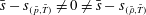
 $$\begin{eqnarray}\displaystyle {\displaystyle \frac{s-s_{(\,\bar{p},\bar{T})}}{R_{g}}}\stackrel{\text{(2.6)}\,}{=}{\displaystyle \frac{1}{R_{g}}}\int _{\bar{T}}^{\bar{T}+T^{\prime }}{\displaystyle \frac{c_{p}(T^{\ast })}{T^{\ast }}}\,\text{d}T^{\ast }-\ln \left(1+{\displaystyle \frac{p^{\prime }}{\bar{p}}}\right), & & \displaystyle\end{eqnarray}$$
 $$\begin{eqnarray}\displaystyle {\displaystyle \frac{s-s_{(\bar{\unicode[STIX]{x1D70C}},\bar{T})}}{R_{g}}}\stackrel{\text{(2.6)}}{=}{\displaystyle \frac{1}{R_{g}}}\int _{\bar{T}}^{\bar{T}+T^{\prime }}{\displaystyle \frac{c_{v}(T^{\ast })}{T^{\ast }}}\,\text{d}T^{\ast }-\ln \left(1+{\displaystyle \frac{\unicode[STIX]{x1D70C}^{\prime }}{\bar{\unicode[STIX]{x1D70C}}}}\right), & & \displaystyle\end{eqnarray}$$
 $s_{(\,\bar{p},\bar{T})}$
and
$s_{(\,\bar{p},\bar{T})}$
and
 $s_{(\bar{\unicode[STIX]{x1D70C}},\bar{T})}$
the entropy at the corresponding states, which are to
$s_{(\bar{\unicode[STIX]{x1D70C}},\bar{T})}$
the entropy at the corresponding states, which are to
 $O(\text{CV}_{\unicode[STIX]{x1D70C}^{\prime }}^{2})$
approximately equal to
$O(\text{CV}_{\unicode[STIX]{x1D70C}^{\prime }}^{2})$
approximately equal to
 $\bar{s}$
(Lele Reference Lele1994, p. 224). Relations (2.7) can be easily expanded in powers series of relative fluctuation amplitudes, and replacing
$\bar{s}$
(Lele Reference Lele1994, p. 224). Relations (2.7) can be easily expanded in powers series of relative fluctuation amplitudes, and replacing
 $s=\bar{s}+s^{\prime }$
we obtain the expansions for the entropy fluctuations, truncated after the quadratic terms
$s=\bar{s}+s^{\prime }$
we obtain the expansions for the entropy fluctuations, truncated after the quadratic terms  $$\begin{eqnarray}\displaystyle {\displaystyle \frac{s^{\prime }}{R_{g}}} & \stackrel{\text{(2.7a)}}{{\sim}} & \displaystyle {\displaystyle \frac{\breve{\unicode[STIX]{x1D6FE}}}{\breve{\unicode[STIX]{x1D6FE}}-1}}\,\left({\displaystyle \frac{T^{\prime }}{\bar{T}}}-\frac{1}{2}\left({\displaystyle \frac{T^{\prime }}{\bar{T}}}\right)^{2}\right)-\left({\displaystyle \frac{p^{\prime }}{\bar{p}}}-\frac{1}{2}\left({\displaystyle \frac{p^{\prime }}{\bar{p}}}\right)^{2}\right)+\frac{1}{2}\left({\displaystyle \frac{T^{\prime }}{\bar{T}}}\right)^{2}\,{\displaystyle \frac{\bar{T}}{R_{g}}}\left.{\displaystyle \frac{\text{d}c_{p}}{\text{d}T}}\right|_{\bar{T}}\nonumber\\ \displaystyle & & \displaystyle -\,{\displaystyle \frac{\bar{s}-s_{(\,\bar{p},\bar{T})}}{R_{g}}}+O\Bigg(\!\left({\displaystyle \frac{p^{\prime }}{\bar{p}}}\right)^{3},\left({\displaystyle \frac{T^{\prime }}{\bar{T}}}\right)^{3}\Bigg)\end{eqnarray}$$
 $$\begin{eqnarray}\displaystyle & \stackrel{\text{(2.7b)}}{{\sim}} & \displaystyle {\displaystyle \frac{1}{\breve{\unicode[STIX]{x1D6FE}}-1}}\,\left({\displaystyle \frac{T^{\prime }}{\bar{T}}}-\frac{1}{2}\left({\displaystyle \frac{T^{\prime }}{\bar{T}}}\right)^{2}\right)-\left({\displaystyle \frac{\unicode[STIX]{x1D70C}^{\prime }}{\bar{\unicode[STIX]{x1D70C}}}}-\frac{1}{2}\left({\displaystyle \frac{\unicode[STIX]{x1D70C}^{\prime }}{\bar{\unicode[STIX]{x1D70C}}}}\right)^{2}\right)+\frac{1}{2}\left({\displaystyle \frac{T^{\prime }}{\bar{T}}}\right)^{2}\,{\displaystyle \frac{\bar{T}}{R_{g}}}\left.{\displaystyle \frac{\text{d}c_{p}}{\text{d}T}}\right|_{\bar{T}}\nonumber\\ \displaystyle & & \displaystyle -\,{\displaystyle \frac{\bar{s}-s_{(\bar{\unicode[STIX]{x1D70C}},\bar{T})}}{R_{g}}}+O\Bigg(\!\left({\displaystyle \frac{\unicode[STIX]{x1D70C}^{\prime }}{\bar{\unicode[STIX]{x1D70C}}}}\right)^{3},\left({\displaystyle \frac{T^{\prime }}{\bar{T}}}\right)^{3}\Bigg),\end{eqnarray}$$
where we defined for brevity
 $$\begin{eqnarray}\displaystyle \breve{\unicode[STIX]{x1D6FE}}:=\unicode[STIX]{x1D6FE}(\bar{T}) & & \displaystyle\end{eqnarray}$$
following the convention that
 $\breve{\cdot }$
is a function of averaged quantities which cannot be identified with a Reynolds or Favre average (Gerolymos & Vallet Reference Gerolymos and Vallet1996, Reference Gerolymos and Vallet2014). Notice the presence of the constants
$\breve{\cdot }$
is a function of averaged quantities which cannot be identified with a Reynolds or Favre average (Gerolymos & Vallet Reference Gerolymos and Vallet1996, Reference Gerolymos and Vallet2014). Notice the presence of the constants
 $\bar{s}-s_{(\,\bar{p},\bar{T})}\neq 0\neq \bar{s}-s_{(\bar{\unicode[STIX]{x1D70C}},\bar{T})}$
, which are
$\bar{s}-s_{(\,\bar{p},\bar{T})}\neq 0\neq \bar{s}-s_{(\bar{\unicode[STIX]{x1D70C}},\bar{T})}$
, which are
 $O(\text{CV}_{\unicode[STIX]{x1D70C}^{\prime }}^{2})$
(Lele Reference Lele1994, p. 224), and are directly related to the nonlinearity of (2.7). The influence of variable
$O(\text{CV}_{\unicode[STIX]{x1D70C}^{\prime }}^{2})$
(Lele Reference Lele1994, p. 224), and are directly related to the nonlinearity of (2.7). The influence of variable
 $c_{p}(T)=R_{g}-c_{v}(T)$
(1.1) also induces a quadratic
$c_{p}(T)=R_{g}-c_{v}(T)$
(1.1) also induces a quadratic
 $O(\text{CV}_{\unicode[STIX]{x1D70C}^{\prime }}^{2})$
term in the expressions for
$O(\text{CV}_{\unicode[STIX]{x1D70C}^{\prime }}^{2})$
term in the expressions for
 $s^{\prime }$
(2.8). Therefore, leading-order approximations related to
$s^{\prime }$
(2.8). Therefore, leading-order approximations related to
 $s^{\prime }$
are valid independently of the variability of
$s^{\prime }$
are valid independently of the variability of
 $c_{p}(T)$
, and depend only on the local value of
$c_{p}(T)$
, and depend only on the local value of
 $\unicode[STIX]{x1D6FE}(\bar{T})$
(1.1). Notice that by (1.1)
$\unicode[STIX]{x1D6FE}(\bar{T})$
(1.1). Notice that by (1.1)
 $d_{T}c_{p}=d_{T}c_{v}$
.
$d_{T}c_{p}=d_{T}c_{v}$
.
2.5 Entropy variance and correlations
It is straightforward from (2.8) to calculate expansions for the entropy variance
 $s_{rms}^{\prime }$
and for correlation coefficients containing
$s_{rms}^{\prime }$
and for correlation coefficients containing
 $s^{\prime }$
. Squaring and averaging (2.8b
) and introducing definitions (2.1), (2.3) yields after simple calculations using (4.4), (A1)
$s^{\prime }$
. Squaring and averaging (2.8b
) and introducing definitions (2.1), (2.3) yields after simple calculations using (4.4), (A1)
 $$\begin{eqnarray}\displaystyle & & \displaystyle \left({\displaystyle \frac{s_{rms}^{\prime }}{R_{g}}}\right)^{2}\stackrel{\text{(2.8b)},\,\text{(4.4)},\,\text{(A 1)},\text{(2.2)}}{{\sim}}{\displaystyle \frac{\breve{\unicode[STIX]{x1D6FE}}}{(\breve{\unicode[STIX]{x1D6FE}}-1)^{2}}}\,\text{CV}_{T^{\prime }}^{2}+{\displaystyle \frac{\breve{\unicode[STIX]{x1D6FE}}}{\breve{\unicode[STIX]{x1D6FE}}-1}}\,\text{CV}_{\unicode[STIX]{x1D70C}^{\prime }}^{2}-{\displaystyle \frac{1}{\breve{\unicode[STIX]{x1D6FE}}-1}}\,\text{CV}_{p^{\prime }}^{2}\nonumber\\ \displaystyle & & \displaystyle \quad -\,{\displaystyle \frac{\breve{\unicode[STIX]{x1D6FE}}}{(\breve{\unicode[STIX]{x1D6FE}}-1)^{2}}}\,S_{T^{\prime }}\,\text{CV}_{T^{\prime }}^{3}-{\displaystyle \frac{\breve{\unicode[STIX]{x1D6FE}}}{\breve{\unicode[STIX]{x1D6FE}}-1}}\,S_{\unicode[STIX]{x1D70C}^{\prime }}\,\text{CV}_{\unicode[STIX]{x1D70C}^{\prime }}^{3}+{\displaystyle \frac{1}{\breve{\unicode[STIX]{x1D6FE}}-1}}\,S_{p^{\prime }}\,\text{CV}_{p^{\prime }}^{3}\nonumber\\ \displaystyle & & \displaystyle \quad +\,c_{s^{\prime }T^{\prime }T^{\prime }}\,{\displaystyle \frac{s_{rms}^{\prime }}{R_{g}}}\,\text{CV}_{T^{\prime }}^{2}\,{\displaystyle \frac{\bar{T}}{R_{g}}}\left.{\displaystyle \frac{\text{d}c_{p}}{\text{d}T}}\right|_{\bar{T}}+O(\text{CV}_{\unicode[STIX]{x1D70C}^{\prime }}^{4}).\end{eqnarray}$$
Notice that (2.9) implies that the correct non-dimensional expression for the entropy variance is
 $R_{g}^{-1}s_{rms}^{\prime }$
and is of the same order of magnitude as the coefficients of variation of the basic thermodynamic quantities. The reason why
$R_{g}^{-1}s_{rms}^{\prime }$
and is of the same order of magnitude as the coefficients of variation of the basic thermodynamic quantities. The reason why
 $R_{g}^{-1}\,s_{rms}^{\prime }$
should be considered in the order-of-magnitude relation (2.2) instead of
$R_{g}^{-1}\,s_{rms}^{\prime }$
should be considered in the order-of-magnitude relation (2.2) instead of
 $\text{CV}_{s^{\prime }}$
is because, by definition (2.6), entropy is defined with respect to an arbitrary reference state, so that the precise value of
$\text{CV}_{s^{\prime }}$
is because, by definition (2.6), entropy is defined with respect to an arbitrary reference state, so that the precise value of
 $\bar{s}$
that appears in the definition of
$\bar{s}$
that appears in the definition of
 $\text{CV}_{s^{\prime }}$
(2.1) has no physical significance: only entropy differences have physical meaning.
$\text{CV}_{s^{\prime }}$
(2.1) has no physical significance: only entropy differences have physical meaning.
3 DNS data
The expansions and approximations developed in the paper are assessed against DNS data from two different aerodynamic configurations, viz sustained compressible HIT (Donzis & Jagannathan Reference Donzis and Jagannathan2013, isotropic homogeneous turbulence) and fully developed compressible turbulent plane channel flow (Gerolymos & Vallet Reference Gerolymos and Vallet2014). In both databases, the coefficient of variation of density
 $\text{CV}_{\unicode[STIX]{x1D70C}^{\prime }}$
(2.1b–d
) increases from very low values (which approach asymptotically the quasi-incompressible limit) to maximum values as high as 0.16 (figure 1). In both cases
$\text{CV}_{\unicode[STIX]{x1D70C}^{\prime }}$
(2.1b–d
) increases from very low values (which approach asymptotically the quasi-incompressible limit) to maximum values as high as 0.16 (figure 1). In both cases
 $\text{CV}_{\unicode[STIX]{x1D70C}^{\prime }}$
varies with the representative Mach number, viz the turbulent Mach number
$\text{CV}_{\unicode[STIX]{x1D70C}^{\prime }}$
varies with the representative Mach number, viz the turbulent Mach number
 $M_{T}$
in HIT (3.1a
) or the centreline Mach number
$M_{T}$
in HIT (3.1a
) or the centreline Mach number
 $\bar{M}_{CL}$
in channel flow (3.2a
).
$\bar{M}_{CL}$
in channel flow (3.2a
).

Figure 1. Log scale plots of DNS data, for the evolution of
 $\text{CV}_{\unicode[STIX]{x1D70C}^{\prime }}$
versus
$\text{CV}_{\unicode[STIX]{x1D70C}^{\prime }}$
versus
 $M_{T}\in [0.1,0.6]$
in sustained homogeneous isotropic turbulence (HIT) simulations (Donzis & Jagannathan Reference Donzis and Jagannathan2013; D. A. Donzis, 2016 Compressible HIT DNS data, Private communication, donzis@tamu.edu; Jagannathan & Donzis Reference Jagannathan and Donzis2016), and for the evolution of
$M_{T}\in [0.1,0.6]$
in sustained homogeneous isotropic turbulence (HIT) simulations (Donzis & Jagannathan Reference Donzis and Jagannathan2013; D. A. Donzis, 2016 Compressible HIT DNS data, Private communication, donzis@tamu.edu; Jagannathan & Donzis Reference Jagannathan and Donzis2016), and for the evolution of
 $\text{CV}_{\unicode[STIX]{x1D70C}^{\prime }}$
versus
$\text{CV}_{\unicode[STIX]{x1D70C}^{\prime }}$
versus
 $\bar{M}_{CL}\in [0.3,2.5]$
in fully developed compressible turbulent plane channel (TPC) flow (Gerolymos & Vallet Reference Gerolymos and Vallet2014) at three different locations across the channel (wall, centreline and maximum value).
$\bar{M}_{CL}\in [0.3,2.5]$
in fully developed compressible turbulent plane channel (TPC) flow (Gerolymos & Vallet Reference Gerolymos and Vallet2014) at three different locations across the channel (wall, centreline and maximum value).
Donzis & Jagannathan (Reference Donzis and Jagannathan2013, figure 2, p. 227) have estimated that in HIT
 $\text{CV}_{\unicode[STIX]{x1D70C}^{\prime }}$
increases as
$\text{CV}_{\unicode[STIX]{x1D70C}^{\prime }}$
increases as
 $M_{T}^{2.2}$
, the exponent being a best fit of the data. A slightly lower exponent of
$M_{T}^{2.2}$
, the exponent being a best fit of the data. A slightly lower exponent of
 $2.1$
also fits well the DNS data (figure 1). The channel DNS data (Gerolymos & Vallet Reference Gerolymos and Vallet2014) indicate that
$2.1$
also fits well the DNS data (figure 1). The channel DNS data (Gerolymos & Vallet Reference Gerolymos and Vallet2014) indicate that
 $\text{CV}_{\unicode[STIX]{x1D70C}^{\prime }}$
varies as
$\text{CV}_{\unicode[STIX]{x1D70C}^{\prime }}$
varies as
 $\bar{M}_{CL}^{2.1}$
(figure 1). The channel data fit very closely the
$\bar{M}_{CL}^{2.1}$
(figure 1). The channel data fit very closely the
 $\bar{M}_{CL}^{2.1}$
variation both at the maximum near-wall peak and at the channel centreline, but exhibit some scatter at the wall. This is attributed to a
$\bar{M}_{CL}^{2.1}$
variation both at the maximum near-wall peak and at the channel centreline, but exhibit some scatter at the wall. This is attributed to a
 $Re_{\unicode[STIX]{x1D70F}^{\star }}$
-influence, associated with the strictly isothermal wall boundary condition, which implies (Gerolymos & Vallet Reference Gerolymos and Vallet2014, (3.5), p. 719)
$Re_{\unicode[STIX]{x1D70F}^{\star }}$
-influence, associated with the strictly isothermal wall boundary condition, which implies (Gerolymos & Vallet Reference Gerolymos and Vallet2014, (3.5), p. 719)
 $[p_{rms}^{\prime }]_{w}=a_{w}^{2}[\unicode[STIX]{x1D70C}_{rms}^{\prime }]_{w}\;\Longleftrightarrow \;[\text{CV}_{p^{\prime }}]_{w}=\unicode[STIX]{x1D6FE}_{w}[\text{CV}_{\unicode[STIX]{x1D70C}^{\prime }}]_{w}$
; therefore,
$[p_{rms}^{\prime }]_{w}=a_{w}^{2}[\unicode[STIX]{x1D70C}_{rms}^{\prime }]_{w}\;\Longleftrightarrow \;[\text{CV}_{p^{\prime }}]_{w}=\unicode[STIX]{x1D6FE}_{w}[\text{CV}_{\unicode[STIX]{x1D70C}^{\prime }}]_{w}$
; therefore,
 $[\text{CV}_{\unicode[STIX]{x1D70C}^{\prime }}]_{w}$
follows the well known from incompressible channel flow (Tsuji et al.
Reference Tsuji, Fransson, Alfredsson and Johansson2007)
$[\text{CV}_{\unicode[STIX]{x1D70C}^{\prime }}]_{w}$
follows the well known from incompressible channel flow (Tsuji et al.
Reference Tsuji, Fransson, Alfredsson and Johansson2007)
 $Re_{\unicode[STIX]{x1D70F}^{\star }}$
-dependence of
$Re_{\unicode[STIX]{x1D70F}^{\star }}$
-dependence of
 $[p_{rms}^{\prime }]_{w}^{+}$
.
$[p_{rms}^{\prime }]_{w}^{+}$
.
As a conclusion, aerodynamic (
 $\unicode[STIX]{x1D6FE}=1.4$
) DNS data indicate that
$\unicode[STIX]{x1D6FE}=1.4$
) DNS data indicate that
 $\text{CV}_{\unicode[STIX]{x1D70C}^{\prime }}$
values for a given configuration, vary, at constant
$\text{CV}_{\unicode[STIX]{x1D70C}^{\prime }}$
values for a given configuration, vary, at constant
 $Re$
-number, proportionally to a power of the representative Mach number, with exponent
$Re$
-number, proportionally to a power of the representative Mach number, with exponent
 $\in [2.1,2.2]$
, i.e. slightly higher than 2.
$\in [2.1,2.2]$
, i.e. slightly higher than 2.
3.1 Sustained compressible HIT
Donzis & Jagannathan (Reference Donzis and Jagannathan2013) and Jagannathan & Donzis (Reference Jagannathan and Donzis2016) have performed DNS of sustained compressible HIT with solenoidal forcing at the large scales (Eswaran & Pope Reference Eswaran and Pope1988). The flow is modelled by the compressible Navier–Stokes equations (Jagannathan & Donzis Reference Jagannathan and Donzis2016, (3.1–3.5), p. 673), without bulk viscosity
 $\unicode[STIX]{x1D707}_{b}=0$
(Gerolymos & Vallet Reference Gerolymos and Vallet2014, (2.1e), p. 706), a power law for the dynamic viscosity
$\unicode[STIX]{x1D707}_{b}=0$
(Gerolymos & Vallet Reference Gerolymos and Vallet2014, (2.1e), p. 706), a power law for the dynamic viscosity
 $\unicode[STIX]{x1D707}(T)\propto \sqrt{T}$
and constant Prandtl number
$\unicode[STIX]{x1D707}(T)\propto \sqrt{T}$
and constant Prandtl number
 $Pr=0.72$
(Donzis & Jagannathan Reference Donzis and Jagannathan2013, p. 224). The working medium follows the equation of state (1.1) with a constant ratio of specific heats (1.1)
$Pr=0.72$
(Donzis & Jagannathan Reference Donzis and Jagannathan2013, p. 224). The working medium follows the equation of state (1.1) with a constant ratio of specific heats (1.1)
 $\unicode[STIX]{x1D6FE}=1.4$
(Donzis & Jagannathan Reference Donzis and Jagannathan2013, figure 7, p. 234). The representative parameters in this configuration are the turbulent Mach number
$\unicode[STIX]{x1D6FE}=1.4$
(Donzis & Jagannathan Reference Donzis and Jagannathan2013, figure 7, p. 234). The representative parameters in this configuration are the turbulent Mach number
 $M_{T}$
(Jagannathan & Donzis Reference Jagannathan and Donzis2016, p. 670) and the Taylor-microscale Reynolds number
$M_{T}$
(Jagannathan & Donzis Reference Jagannathan and Donzis2016, p. 670) and the Taylor-microscale Reynolds number
 $Re_{\unicode[STIX]{x1D706}}$
(Jagannathan & Donzis Reference Jagannathan and Donzis2016, p. 671)
$Re_{\unicode[STIX]{x1D706}}$
(Jagannathan & Donzis Reference Jagannathan and Donzis2016, p. 671)
 $$\begin{eqnarray}\displaystyle M_{T}:={\displaystyle \frac{\sqrt{\overline{u_{i}^{\prime }u_{i}^{\prime }}}}{\bar{a}}}={\displaystyle \frac{u_{rms}^{\prime }\sqrt{3}}{\bar{a}}}, & & \displaystyle\end{eqnarray}$$
 $$\begin{eqnarray}\displaystyle Re_{\unicode[STIX]{x1D706}}:={\displaystyle \frac{\bar{\unicode[STIX]{x1D70C}}\,\sqrt{u_{rms}^{\prime }}\,\unicode[STIX]{x1D706}_{\Vert }}{\bar{\unicode[STIX]{x1D707}}}};\quad \unicode[STIX]{x1D706}_{\Vert }:=\sqrt{{\displaystyle \frac{\overline{{u^{\prime }}^{2}}}{\overline{\left({\displaystyle \frac{\unicode[STIX]{x2202}u^{\prime }}{\unicode[STIX]{x2202}x}}\right)^{2}}}}}. & & \displaystyle\end{eqnarray}$$
These data were made available with a precision of 4 significant digits (D. A. Donzis, 2016, Private communication, lower precision was found inadequate for use in the approximate relations developed in the paper), and cover the range
 $Re_{\unicode[STIX]{x1D706}}\in [35,430]$
and
$Re_{\unicode[STIX]{x1D706}}\in [35,430]$
and
 $M_{T}\in [0.1,0.6]$
, with a corresponding range of
$M_{T}\in [0.1,0.6]$
, with a corresponding range of
 $\text{CV}_{\unicode[STIX]{x1D70C}^{\prime }}\in [0.004,0.157]$
(Donzis & Jagannathan Reference Donzis and Jagannathan2013, table 1, p. 225). The ratios
$\text{CV}_{\unicode[STIX]{x1D70C}^{\prime }}\in [0.004,0.157]$
(Donzis & Jagannathan Reference Donzis and Jagannathan2013, table 1, p. 225). The ratios
 $\text{CV}_{\unicode[STIX]{x1D70C}^{\prime }}^{-1}\text{CV}_{p^{\prime }}$
and
$\text{CV}_{\unicode[STIX]{x1D70C}^{\prime }}^{-1}\text{CV}_{p^{\prime }}$
and
 $\text{CV}_{\unicode[STIX]{x1D70C}^{\prime }}^{-1}\text{CV}_{T^{\prime }}$
vary slightly with
$\text{CV}_{\unicode[STIX]{x1D70C}^{\prime }}^{-1}\text{CV}_{T^{\prime }}$
vary slightly with
 $M_{T}$
and
$M_{T}$
and
 $Re_{\unicode[STIX]{x1D706}}$
(figure 2). This dependency notwithstanding, in this flow, relative variations of temperature are weaker than relative variations of density (
$Re_{\unicode[STIX]{x1D706}}$
(figure 2). This dependency notwithstanding, in this flow, relative variations of temperature are weaker than relative variations of density (
 $0.35\,\text{CV}_{\unicode[STIX]{x1D70C}^{\prime }}\lessapprox \text{CV}_{T^{\prime }}\lessapprox 0.4\,\text{CV}_{\unicode[STIX]{x1D70C}^{\prime }}$
; figure 2) whereas relative variations of pressure are stronger (
$0.35\,\text{CV}_{\unicode[STIX]{x1D70C}^{\prime }}\lessapprox \text{CV}_{T^{\prime }}\lessapprox 0.4\,\text{CV}_{\unicode[STIX]{x1D70C}^{\prime }}$
; figure 2) whereas relative variations of pressure are stronger (
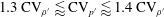 $1.3\,\text{CV}_{\unicode[STIX]{x1D70C}^{\prime }}\lessapprox \text{CV}_{p^{\prime }}\lessapprox 1.4\,\text{CV}_{\unicode[STIX]{x1D70C}^{\prime }}$
; figure 2).
$1.3\,\text{CV}_{\unicode[STIX]{x1D70C}^{\prime }}\lessapprox \text{CV}_{p^{\prime }}\lessapprox 1.4\,\text{CV}_{\unicode[STIX]{x1D70C}^{\prime }}$
; figure 2).

Figure 2. Sustained homogeneous isotropic turbulence (HIT) DNS data (Donzis & Jagannathan Reference Donzis and Jagannathan2013; D. A. Donzis, 2016, Private communication; Jagannathan & Donzis Reference Jagannathan and Donzis2016) for the magnitude of the ratios of the coefficients of variation of temperature
 $\text{CV}_{T^{\prime }}$
and pressure
$\text{CV}_{T^{\prime }}$
and pressure
 $\text{CV}_{p^{\prime }}$
to the coefficient of variation of density
$\text{CV}_{p^{\prime }}$
to the coefficient of variation of density
 $\text{CV}_{\unicode[STIX]{x1D70C}^{\prime }}$
, as a function of the turbulent Mach number
$\text{CV}_{\unicode[STIX]{x1D70C}^{\prime }}$
, as a function of the turbulent Mach number
 $M_{T}\in [0.1,0.6]$
, for different values of
$M_{T}\in [0.1,0.6]$
, for different values of
 $Re_{\unicode[STIX]{x1D706}}\in [35,430]$
.
$Re_{\unicode[STIX]{x1D706}}\in [35,430]$
.
3.2 Compressible turbulent plane channel flow
The DNS data for compressible turbulent plane channel flow were obtained (Gerolymos & Vallet Reference Gerolymos and Vallet2014) using a high-order solver (Gerolymos, Sénéchal & Vallet Reference Gerolymos, Sénéchal and Vallet2010). The flow is modelled by the compressible Navier–Stokes equations (Gerolymos & Vallet Reference Gerolymos and Vallet2014, (2.1), p. 706), without bulk viscosity
 $\unicode[STIX]{x1D707}_{b}=0$
(Gerolymos & Vallet Reference Gerolymos and Vallet2014, (2.1e), p. 706). The working medium is air, following the equation of state (1.1) with a constant ratio of specific heats (1.1)
$\unicode[STIX]{x1D707}_{b}=0$
(Gerolymos & Vallet Reference Gerolymos and Vallet2014, (2.1e), p. 706). The working medium is air, following the equation of state (1.1) with a constant ratio of specific heats (1.1)
 $\unicode[STIX]{x1D6FE}=1.4$
, and Sutherland-like laws for the dynamic viscosity
$\unicode[STIX]{x1D6FE}=1.4$
, and Sutherland-like laws for the dynamic viscosity
 $\unicode[STIX]{x1D707}(T)$
and heat conductivity
$\unicode[STIX]{x1D707}(T)$
and heat conductivity
 $\unicode[STIX]{x1D706}(T)$
(Gerolymos & Vallet Reference Gerolymos and Vallet2014, p. 706). The data used in the paper include both data from these computations (Gerolymos & Vallet Reference Gerolymos and Vallet2014) and new unpublished data (table 1). The relevant Mach number is the mean centreline Mach number (Gerolymos & Vallet Reference Gerolymos and Vallet2014, figure 1, p. 713)
$\unicode[STIX]{x1D706}(T)$
(Gerolymos & Vallet Reference Gerolymos and Vallet2014, p. 706). The data used in the paper include both data from these computations (Gerolymos & Vallet Reference Gerolymos and Vallet2014) and new unpublished data (table 1). The relevant Mach number is the mean centreline Mach number (Gerolymos & Vallet Reference Gerolymos and Vallet2014, figure 1, p. 713)
 $$\begin{eqnarray}\displaystyle \bar{M}_{CL}:=\overline{\left({\displaystyle \frac{u_{CL}}{a_{CL}}}\right)}, & & \displaystyle\end{eqnarray}$$
 $u$
is the streamwise velocity,
$u$
is the streamwise velocity,
 $a$
is the sound speed and
$a$
is the sound speed and
 $(\cdot )_{CL}$
denotes values at the centreline
$(\cdot )_{CL}$
denotes values at the centreline
 $y=\unicode[STIX]{x1D6FF}$
. Following Huang et al. (Reference Huang, Coleman and Bradshaw1995) we use mixed wall-local scaling (HCB-scaling), based on skin friction
$y=\unicode[STIX]{x1D6FF}$
. Following Huang et al. (Reference Huang, Coleman and Bradshaw1995) we use mixed wall-local scaling (HCB-scaling), based on skin friction
 $\bar{\unicode[STIX]{x1D70F}}_{w}$
along with the local mean density
$\bar{\unicode[STIX]{x1D70F}}_{w}$
along with the local mean density
 $\bar{\unicode[STIX]{x1D70C}}(y)$
and mean viscosity
$\bar{\unicode[STIX]{x1D70C}}(y)$
and mean viscosity
 $\bar{\unicode[STIX]{x1D707}}(y)$
, for the non-dimensional wall distance and corresponding Reynolds number
$\bar{\unicode[STIX]{x1D707}}(y)$
, for the non-dimensional wall distance and corresponding Reynolds number  $$\begin{eqnarray}\displaystyle y^{\star }:={\displaystyle \frac{\bar{\unicode[STIX]{x1D70C}}(y)\sqrt{{\displaystyle \frac{\bar{\unicode[STIX]{x1D70F}}_{w}}{\bar{\unicode[STIX]{x1D70C}}(y)}}}(y-y_{w})}{\bar{\unicode[STIX]{x1D707}}(y)}}={\displaystyle \frac{\sqrt{\bar{\unicode[STIX]{x1D70C}}^{+}(y)}}{\bar{\unicode[STIX]{x1D707}}^{+}(y)}}y^{+};\quad Re_{\unicode[STIX]{x1D70F}^{\star }}:=\unicode[STIX]{x1D6FF}^{\star }={\displaystyle \frac{\sqrt{\bar{\unicode[STIX]{x1D70C}}_{CL}^{+}}}{\bar{\unicode[STIX]{x1D707}}_{CL}^{+}}}\unicode[STIX]{x1D6FF}^{+}, & & \displaystyle\end{eqnarray}$$
where
 $(\cdot )_{w}$
denotes wall values and
$(\cdot )_{w}$
denotes wall values and
 $$\begin{eqnarray}\displaystyle y^{+}:={\displaystyle \frac{\bar{\unicode[STIX]{x1D70C}}_{w}\sqrt{{\displaystyle \frac{\bar{\unicode[STIX]{x1D70F}}_{w}}{\bar{\unicode[STIX]{x1D70C}}_{w}}}}(y-y_{w})}{\bar{\unicode[STIX]{x1D707}}_{w}}};\quad Re_{\unicode[STIX]{x1D70F}_{w}}:=\unicode[STIX]{x1D6FF}^{+};\quad \bar{\unicode[STIX]{x1D70C}}^{+}:={\displaystyle \frac{\bar{\unicode[STIX]{x1D70C}}}{\bar{\unicode[STIX]{x1D70C}}_{w}}};\quad \bar{\unicode[STIX]{x1D707}}^{+}:={\displaystyle \frac{\bar{\unicode[STIX]{x1D707}}}{\bar{\unicode[STIX]{x1D707}}_{w}}} & & \displaystyle\end{eqnarray}$$
are the usual incompressible-flow inner-scaled variables (Gerolymos & Vallet Reference Gerolymos and Vallet2014, (3.2), p. 714).
Table 1. Parameters of the DNS computations (
 $L_{x}$
,
$L_{x}$
,
 $L_{y}$
,
$L_{y}$
,
 $L_{z}$
(
$L_{z}$
(
 $N_{x}$
,
$N_{x}$
,
 $N_{y}$
,
$N_{y}$
,
 $N_{z}$
) are the dimensions (number of grid points) of the computational domain (
$N_{z}$
) are the dimensions (number of grid points) of the computational domain (
 $x=$
homogeneous streamwise,
$x=$
homogeneous streamwise,
 $y=$
wall-normal,
$y=$
wall-normal,
 $z=$
homogeneous spanwise direction);
$z=$
homogeneous spanwise direction);
 $\unicode[STIX]{x1D6FF}$
is the channel half-height;
$\unicode[STIX]{x1D6FF}$
is the channel half-height;
 $(\cdot )^{+}$
denotes wall units;
$(\cdot )^{+}$
denotes wall units;
 $\unicode[STIX]{x0394}x^{+}$
,
$\unicode[STIX]{x0394}x^{+}$
,
 $\unicode[STIX]{x0394}y_{w}^{+}$
,
$\unicode[STIX]{x0394}y_{w}^{+}$
,
 $\unicode[STIX]{x0394}y_{CL}^{+}$
,
$\unicode[STIX]{x0394}y_{CL}^{+}$
,
 $\unicode[STIX]{x0394}z^{+}$
are the mesh sizes;
$\unicode[STIX]{x0394}z^{+}$
are the mesh sizes;
 $(\cdot )_{w}$
denotes wall and
$(\cdot )_{w}$
denotes wall and
 $(\cdot )_{CL}$
centreline values;
$(\cdot )_{CL}$
centreline values;
 $N_{y^{+}\leqslant 10}$
is the number of grid points between the wall and
$N_{y^{+}\leqslant 10}$
is the number of grid points between the wall and
 $y^{+}=10$
;
$y^{+}=10$
;
 $\bar{M}_{CL}$
is the centreline Mach number (3.2a
);
$\bar{M}_{CL}$
is the centreline Mach number (3.2a
);
 $Re_{\unicode[STIX]{x1D70F}^{\star }}:=\sqrt{\bar{\unicode[STIX]{x1D70C}}_{CL}\,\bar{\unicode[STIX]{x1D70F}}_{w}}\unicode[STIX]{x1D6FF}\bar{\unicode[STIX]{x1D707}}_{CL}^{-1}$
is the friction Reynolds number in HCB-scaling (3.2b,c
);
$Re_{\unicode[STIX]{x1D70F}^{\star }}:=\sqrt{\bar{\unicode[STIX]{x1D70C}}_{CL}\,\bar{\unicode[STIX]{x1D70F}}_{w}}\unicode[STIX]{x1D6FF}\bar{\unicode[STIX]{x1D707}}_{CL}^{-1}$
is the friction Reynolds number in HCB-scaling (3.2b,c
);
 $Re_{\unicode[STIX]{x1D70F}_{w}}:=\sqrt{\bar{\unicode[STIX]{x1D70C}}_{w}\,\bar{\unicode[STIX]{x1D70F}}_{w}}\unicode[STIX]{x1D6FF}\bar{\unicode[STIX]{x1D707}}_{w}^{-1}$
is the friction Reynolds number (3.2d–g
);
$Re_{\unicode[STIX]{x1D70F}_{w}}:=\sqrt{\bar{\unicode[STIX]{x1D70C}}_{w}\,\bar{\unicode[STIX]{x1D70F}}_{w}}\unicode[STIX]{x1D6FF}\bar{\unicode[STIX]{x1D707}}_{w}^{-1}$
is the friction Reynolds number (3.2d–g
);
 $\unicode[STIX]{x0394}t^{+}$
is the computational time step;
$\unicode[STIX]{x0394}t^{+}$
is the computational time step;
 $t_{\text{OBS}}^{+}$
is the observation period over which single-point statistics were computed;
$t_{\text{OBS}}^{+}$
is the observation period over which single-point statistics were computed;
 $\unicode[STIX]{x0394}t_{s}^{+}$
is the sampling time step for the single-point statistics).
$\unicode[STIX]{x0394}t_{s}^{+}$
is the sampling time step for the single-point statistics).

The coefficients of variation
 $\{\text{CV}_{p^{\prime }},\text{CV}_{\unicode[STIX]{x1D70C}^{\prime }},\text{CV}_{T^{\prime }}\}$
are of the same order of magnitude everywhere in the channel (figure 3), and for all
$\{\text{CV}_{p^{\prime }},\text{CV}_{\unicode[STIX]{x1D70C}^{\prime }},\text{CV}_{T^{\prime }}\}$
are of the same order of magnitude everywhere in the channel (figure 3), and for all
 $(Re_{\unicode[STIX]{x1D70F}^{\star }},\bar{M}_{CL})$
that were investigated, even at the low Mach number limit. Notice that previously published results (Gerolymos & Vallet Reference Gerolymos and Vallet2014, figure 6, p. 721) indicate that the correlation coefficients between thermodynamic variables plotted against
$(Re_{\unicode[STIX]{x1D70F}^{\star }},\bar{M}_{CL})$
that were investigated, even at the low Mach number limit. Notice that previously published results (Gerolymos & Vallet Reference Gerolymos and Vallet2014, figure 6, p. 721) indicate that the correlation coefficients between thermodynamic variables plotted against
 $y^{\star }$
(3.2b,c
) show little dependence on
$y^{\star }$
(3.2b,c
) show little dependence on
 $\bar{M}_{CL}$
, except perhaps very near the wall (
$\bar{M}_{CL}$
, except perhaps very near the wall (
 $y^{\star }<10$
). Nonetheless, in the neighbourhood of the near-wall
$y^{\star }<10$
). Nonetheless, in the neighbourhood of the near-wall
 $\text{CV}_{\unicode[STIX]{x1D70C}^{\prime }}$
peak (Gerolymos & Vallet Reference Gerolymos and Vallet2014,
$\text{CV}_{\unicode[STIX]{x1D70C}^{\prime }}$
peak (Gerolymos & Vallet Reference Gerolymos and Vallet2014,
 $7\lessapprox y^{\ast }\lessapprox 20$
, figure 5, p. 720),
$7\lessapprox y^{\ast }\lessapprox 20$
, figure 5, p. 720),
 $\text{CV}_{\unicode[STIX]{x1D70C}^{\prime }}\approxeq 5\text{CV}_{p^{\prime }}$
(figure 3), so that the assumption
$\text{CV}_{\unicode[STIX]{x1D70C}^{\prime }}\approxeq 5\text{CV}_{p^{\prime }}$
(figure 3), so that the assumption
 $O(\text{CV}_{\unicode[STIX]{x1D70C}^{\prime }})=O(\text{CV}_{p^{\prime }})$
(2.2) is stretched to the limit. On the contrary,
$O(\text{CV}_{\unicode[STIX]{x1D70C}^{\prime }})=O(\text{CV}_{p^{\prime }})$
(2.2) is stretched to the limit. On the contrary,
 $O(\text{CV}_{\unicode[STIX]{x1D70C}^{\prime }})=O(\text{CV}_{T^{\prime }})$
is satisfied practically everywhere, except very near the wall (
$O(\text{CV}_{\unicode[STIX]{x1D70C}^{\prime }})=O(\text{CV}_{T^{\prime }})$
is satisfied practically everywhere, except very near the wall (
 $y^{\star }\lessapprox 1$
; figure 3) where the strictly isothermal wall boundary condition enforces
$y^{\star }\lessapprox 1$
; figure 3) where the strictly isothermal wall boundary condition enforces
 $[\text{CV}_{T^{\prime }}]_{w}=0$
at the wall (
$[\text{CV}_{T^{\prime }}]_{w}=0$
at the wall (
 $y^{\ast }=0$
). The question is naturally raised, how a less stringent isothermal-in-the-mean wall boundary condition, where
$y^{\ast }=0$
). The question is naturally raised, how a less stringent isothermal-in-the-mean wall boundary condition, where
 $T_{w}^{\prime }\neq 0$
but instead only
$T_{w}^{\prime }\neq 0$
but instead only
 $\bar{T}_{w}=\text{const.}$
in the mean is enforced, would modify the viscous sublayer thermodynamic turbulence, and this will be the subject of a future study. Nonetheless, DNS data (Gerolymos & Vallet Reference Gerolymos and Vallet2014, figure 5, p. 720) suggest that the boundary condition effect is confined very near the wall (
$\bar{T}_{w}=\text{const.}$
in the mean is enforced, would modify the viscous sublayer thermodynamic turbulence, and this will be the subject of a future study. Nonetheless, DNS data (Gerolymos & Vallet Reference Gerolymos and Vallet2014, figure 5, p. 720) suggest that the boundary condition effect is confined very near the wall (
 $y^{\ast }\lessapprox 1$
), and this is further confirmed in § 6.
$y^{\ast }\lessapprox 1$
), and this is further confirmed in § 6.

Figure 3. Compressible fully developed turbulent plane channel (TPC) flow DNS data (Gerolymos & Vallet Reference Gerolymos and Vallet2014) for the magnitude of the ratios of the coefficients of variation of temperature
 $\text{CV}_{T^{\prime }}$
and pressure
$\text{CV}_{T^{\prime }}$
and pressure
 $\text{CV}_{p^{\prime }}$
to the coefficient of variation of density
$\text{CV}_{p^{\prime }}$
to the coefficient of variation of density
 $\text{CV}_{\unicode[STIX]{x1D70C}^{\prime }}$
, as a function of the HCB-scaled wall distance
$\text{CV}_{\unicode[STIX]{x1D70C}^{\prime }}$
, as a function of the HCB-scaled wall distance
 $y^{\star }$
(3.2b,c
), for different values of
$y^{\star }$
(3.2b,c
), for different values of
 $Re_{\unicode[STIX]{x1D70F}^{\star }}\in [78,341]$
and
$Re_{\unicode[STIX]{x1D70F}^{\star }}\in [78,341]$
and
 $\bar{M}_{CL}\in [0.3,2.5]$
(Gerolymos & Vallet Reference Gerolymos and Vallet2014, the shaded region corresponds to values
$\bar{M}_{CL}\in [0.3,2.5]$
(Gerolymos & Vallet Reference Gerolymos and Vallet2014, the shaded region corresponds to values
 $\text{CV}_{\unicode[STIX]{x1D70C}^{\prime }}\geqslant 2\text{CV}_{p^{\prime }}$
observed in the neighbourhood of the
$\text{CV}_{\unicode[STIX]{x1D70C}^{\prime }}\geqslant 2\text{CV}_{p^{\prime }}$
observed in the neighbourhood of the
 $\text{CV}_{\unicode[STIX]{x1D70C}^{\prime }}$
-peak; figure 5, p. 720).
$\text{CV}_{\unicode[STIX]{x1D70C}^{\prime }}$
-peak; figure 5, p. 720).
3.3 Shear turbulence is not polytropic
Near the centreline, where the wall influence is weak, channel DNS data (figure 3) indicate that the relative magnitudes of the coefficients of variation
 $\{\text{CV}_{\unicode[STIX]{x1D70C}^{\prime }},\text{CV}_{T^{\prime }},\text{CV}_{p^{\prime }}\}$
approach those observed in the HIT DNS data (figure 2), the more so as
$\{\text{CV}_{\unicode[STIX]{x1D70C}^{\prime }},\text{CV}_{T^{\prime }},\text{CV}_{p^{\prime }}\}$
approach those observed in the HIT DNS data (figure 2), the more so as
 $Re_{\unicode[STIX]{x1D70F}^{\star }}=\unicode[STIX]{x1D6FF}^{\star }$
(3.2b,c
) increases. On the other hand, close to the wall (
$Re_{\unicode[STIX]{x1D70F}^{\star }}=\unicode[STIX]{x1D6FF}^{\star }$
(3.2b,c
) increases. On the other hand, close to the wall (
 $y^{\star }\lessapprox 100$
) there are substantial differences. Whereas in HIT (figure 2) and near the centreline in channel flow (figure 3),
$y^{\star }\lessapprox 100$
) there are substantial differences. Whereas in HIT (figure 2) and near the centreline in channel flow (figure 3),
 $\text{CV}_{p^{\prime }}>\text{CV}_{\unicode[STIX]{x1D70C}^{\prime }}>\text{CV}_{T^{\prime }}$
, near the solid wall
$\text{CV}_{p^{\prime }}>\text{CV}_{\unicode[STIX]{x1D70C}^{\prime }}>\text{CV}_{T^{\prime }}$
, near the solid wall
 $\text{CV}_{\unicode[STIX]{x1D70C}^{\prime }}\approxeq \text{CV}_{T^{\prime }}>\text{CV}_{p^{\prime }}$
(
$\text{CV}_{\unicode[STIX]{x1D70C}^{\prime }}\approxeq \text{CV}_{T^{\prime }}>\text{CV}_{p^{\prime }}$
(
 $5\lessapprox y^{\star }\lessapprox 50$
; figure 3). This difference is easily explained by the approximate leading-order relation (Donzis & Jagannathan Reference Donzis and Jagannathan2013, (3.4), p. 226)
$5\lessapprox y^{\star }\lessapprox 50$
; figure 3). This difference is easily explained by the approximate leading-order relation (Donzis & Jagannathan Reference Donzis and Jagannathan2013, (3.4), p. 226)
 $\text{CV}_{p^{\prime }}^{2}\approxeq \text{CV}_{\unicode[STIX]{x1D70C}^{\prime }}^{2}+\text{CV}_{T^{\prime }}^{2}+2\,c_{\unicode[STIX]{x1D70C}^{\prime }T^{\prime }}\,\text{CV}_{\unicode[STIX]{x1D70C}^{\prime }}\,\text{CV}_{T^{\prime }}$
(4.4). In HIT (Donzis & Jagannathan Reference Donzis and Jagannathan2013, table 1, p. 225) and in channel flow near the centreline (Gerolymos & Vallet Reference Gerolymos and Vallet2014, figure 6, p. 721), the correlation coefficient (2.3a
)
$\text{CV}_{p^{\prime }}^{2}\approxeq \text{CV}_{\unicode[STIX]{x1D70C}^{\prime }}^{2}+\text{CV}_{T^{\prime }}^{2}+2\,c_{\unicode[STIX]{x1D70C}^{\prime }T^{\prime }}\,\text{CV}_{\unicode[STIX]{x1D70C}^{\prime }}\,\text{CV}_{T^{\prime }}$
(4.4). In HIT (Donzis & Jagannathan Reference Donzis and Jagannathan2013, table 1, p. 225) and in channel flow near the centreline (Gerolymos & Vallet Reference Gerolymos and Vallet2014, figure 6, p. 721), the correlation coefficient (2.3a
)
 $c_{\unicode[STIX]{x1D70C}^{\prime }T^{\prime }}>0\;\Longrightarrow \;\text{CV}_{p^{\prime }}^{2}>\text{CV}_{\unicode[STIX]{x1D70C}^{\prime }}^{2}+\text{CV}_{T^{\prime }}^{2}$
, whereas near the solid wall (Gerolymos & Vallet Reference Gerolymos and Vallet2014,
$c_{\unicode[STIX]{x1D70C}^{\prime }T^{\prime }}>0\;\Longrightarrow \;\text{CV}_{p^{\prime }}^{2}>\text{CV}_{\unicode[STIX]{x1D70C}^{\prime }}^{2}+\text{CV}_{T^{\prime }}^{2}$
, whereas near the solid wall (Gerolymos & Vallet Reference Gerolymos and Vallet2014,
 $y^{\star }\lessapprox 100$
, figure 6, p. 721)
$y^{\star }\lessapprox 100$
, figure 6, p. 721)
 $c_{\unicode[STIX]{x1D70C}^{\prime }T^{\prime }}<0\;\Longrightarrow \;\text{CV}_{p^{\prime }}^{2}<\text{CV}_{\unicode[STIX]{x1D70C}^{\prime }}^{2}+\text{CV}_{T^{\prime }}^{2}$
.
$c_{\unicode[STIX]{x1D70C}^{\prime }T^{\prime }}<0\;\Longrightarrow \;\text{CV}_{p^{\prime }}^{2}<\text{CV}_{\unicode[STIX]{x1D70C}^{\prime }}^{2}+\text{CV}_{T^{\prime }}^{2}$
.

Figure 4. Estimates
 $n_{P}(\text{CV}_{p^{\prime }},\text{CV}_{\unicode[STIX]{x1D70C}^{\prime }})\approxeq n_{P_{p^{\prime }\unicode[STIX]{x1D70C}^{\prime }}}$
and
$n_{P}(\text{CV}_{p^{\prime }},\text{CV}_{\unicode[STIX]{x1D70C}^{\prime }})\approxeq n_{P_{p^{\prime }\unicode[STIX]{x1D70C}^{\prime }}}$
and
 $n_{P}(\text{CV}_{\unicode[STIX]{x1D70C}^{\prime }},\text{CV}_{T^{\prime }})\approxeq n_{P_{\unicode[STIX]{x1D70C}^{\prime }T^{\prime }}}$
by (3.3) of an eventual representative polytropic exponent, from DNS data of sustained homogeneous isotropic turbulence (HIT) simulations (Donzis & Jagannathan Reference Donzis and Jagannathan2013; D. A. Donzis, 2016, Private communication; Jagannathan & Donzis Reference Jagannathan and Donzis2016) versus the turbulent Mach number
$n_{P}(\text{CV}_{\unicode[STIX]{x1D70C}^{\prime }},\text{CV}_{T^{\prime }})\approxeq n_{P_{\unicode[STIX]{x1D70C}^{\prime }T^{\prime }}}$
by (3.3) of an eventual representative polytropic exponent, from DNS data of sustained homogeneous isotropic turbulence (HIT) simulations (Donzis & Jagannathan Reference Donzis and Jagannathan2013; D. A. Donzis, 2016, Private communication; Jagannathan & Donzis Reference Jagannathan and Donzis2016) versus the turbulent Mach number
 $M_{T}\in [0.1,0.6]$
and for compressible fully developed turbulent plane channel (TPC) flow (Gerolymos & Vallet Reference Gerolymos and Vallet2014) versus the HCB-scaled wall distance
$M_{T}\in [0.1,0.6]$
and for compressible fully developed turbulent plane channel (TPC) flow (Gerolymos & Vallet Reference Gerolymos and Vallet2014) versus the HCB-scaled wall distance
 $y^{\star }$
(3.2b,c
) (for different values of
$y^{\star }$
(3.2b,c
) (for different values of
 $Re_{\unicode[STIX]{x1D70F}^{\star }}\in [78,341]$
and
$Re_{\unicode[STIX]{x1D70F}^{\star }}\in [78,341]$
and
 $\bar{M}_{CL}\in [0.3,2.5]$
).
$\bar{M}_{CL}\in [0.3,2.5]$
).
The difference in behaviour between HIT and near-wall turbulence is further highlighted by considering polytropic exponents, in line with Donzis & Jagannathan (Reference Donzis and Jagannathan2013, figure 7, p. 234). If turbulence were polytropic (
 $p\propto \unicode[STIX]{x1D70C}^{n_{P}}$
), then, to leading order, specific relations should hold between CVs (Barre & Bonnet Reference Barre and Bonnet2015, p. 331)
$p\propto \unicode[STIX]{x1D70C}^{n_{P}}$
), then, to leading order, specific relations should hold between CVs (Barre & Bonnet Reference Barre and Bonnet2015, p. 331)
 $$\begin{eqnarray}\displaystyle p\propto \unicode[STIX]{x1D70C}^{n_{P}}\stackrel{\text{(1.1)}}{\;\Longrightarrow \;}n_{P}\approxeq \underbrace{{\displaystyle \frac{\text{CV}_{p^{\prime }}}{\text{CV}_{\unicode[STIX]{x1D70C}^{\prime }}}}}_{\displaystyle n_{P_{p^{\prime }\unicode[STIX]{x1D70C}^{\prime }}}}\approxeq \underbrace{1+{\displaystyle \frac{\text{CV}_{T^{\prime }}}{\text{CV}_{\unicode[STIX]{x1D70C}^{\prime }}}}}_{\displaystyle n_{P_{\unicode[STIX]{x1D70C}^{\prime }T^{\prime }}}>1}. & & \displaystyle\end{eqnarray}$$
Notice that expression (3.3) which is used in compressible turbulence, both for instantaneous fluctuations (Rubesin Reference Rubesin1976) or on the average (Blaisdell et al.
Reference Blaisdell, Mansour and Reynolds1993) is a leading-order approximation of a polytropic process. In practice,
 $n_{P_{p^{\prime }\unicode[STIX]{x1D70C}^{\prime }}}$
and
$n_{P_{p^{\prime }\unicode[STIX]{x1D70C}^{\prime }}}$
and
 $n_{P_{\unicode[STIX]{x1D70C}^{\prime }T^{\prime }}}$
are never equal (3.3). Gatski & Bonnet (Reference Gatski and Bonnet2009, p. 74) suggest considering
$n_{P_{\unicode[STIX]{x1D70C}^{\prime }T^{\prime }}}$
are never equal (3.3). Gatski & Bonnet (Reference Gatski and Bonnet2009, p. 74) suggest considering
 $n_{P_{p^{\prime }\unicode[STIX]{x1D70C}^{\prime }}}$
and
$n_{P_{p^{\prime }\unicode[STIX]{x1D70C}^{\prime }}}$
and
 $n_{P_{\unicode[STIX]{x1D70C}^{\prime }T^{\prime }}}$
(3.3) as independent parameters, but still
$n_{P_{\unicode[STIX]{x1D70C}^{\prime }T^{\prime }}}$
(3.3) as independent parameters, but still
 $n_{P_{p^{\prime }\unicode[STIX]{x1D70C}^{\prime }}}\neq n_{P_{\unicode[STIX]{x1D70C}^{\prime }T^{\prime }}}$
implies that turbulence does not follow a polytropic behaviour.
$n_{P_{p^{\prime }\unicode[STIX]{x1D70C}^{\prime }}}\neq n_{P_{\unicode[STIX]{x1D70C}^{\prime }T^{\prime }}}$
implies that turbulence does not follow a polytropic behaviour.
In HIT both expressions (3.3) are reasonably consistent one with another (figure 4), and although the process is not isentropic the departure from the isentropic value
 $\unicode[STIX]{x1D6FE}=1.4$
is not very large. On the contrary, wall turbulence is very far from isentropic (figure 4). Furthermore, for
$\unicode[STIX]{x1D6FE}=1.4$
is not very large. On the contrary, wall turbulence is very far from isentropic (figure 4). Furthermore, for
 $y^{\star }\lessapprox 100$
, the polytropic exponent estimate
$y^{\star }\lessapprox 100$
, the polytropic exponent estimate
 $n_{P}(\text{CV}_{\unicode[STIX]{x1D70C}^{\prime }},\text{CV}_{T^{\prime }})\approxeq n_{P_{\unicode[STIX]{x1D70C}^{\prime }T^{\prime }}}>1$
is substantially higher than the isentropic value (figure 4), whereas the polytropic exponent estimate
$n_{P}(\text{CV}_{\unicode[STIX]{x1D70C}^{\prime }},\text{CV}_{T^{\prime }})\approxeq n_{P_{\unicode[STIX]{x1D70C}^{\prime }T^{\prime }}}>1$
is substantially higher than the isentropic value (figure 4), whereas the polytropic exponent estimate
 $n_{P}(\text{CV}_{p^{\prime }},\text{CV}_{\unicode[STIX]{x1D70C}^{\prime }})\approxeq n_{P_{p^{\prime }\unicode[STIX]{x1D70C}^{\prime }}}$
is substantially lower than the isentropic value (figure 4). Therefore, not only is wall turbulence not isentropic, but it cannot be approximated by a polytropic process, which would require the two estimates of
$n_{P}(\text{CV}_{p^{\prime }},\text{CV}_{\unicode[STIX]{x1D70C}^{\prime }})\approxeq n_{P_{p^{\prime }\unicode[STIX]{x1D70C}^{\prime }}}$
is substantially lower than the isentropic value (figure 4). Therefore, not only is wall turbulence not isentropic, but it cannot be approximated by a polytropic process, which would require the two estimates of
 $n_{P}$
(3.3) to be approximately the same. It is not always recognized that the equality
$n_{P}$
(3.3) to be approximately the same. It is not always recognized that the equality
 $n_{P_{p^{\prime }\unicode[STIX]{x1D70C}^{\prime }}}\approxeq n_{P_{\unicode[STIX]{x1D70C}^{\prime }T^{\prime }}}$
can only be achieved under very specific conditions. To leading order, straightforward calculation of the difference
$n_{P_{p^{\prime }\unicode[STIX]{x1D70C}^{\prime }}}\approxeq n_{P_{\unicode[STIX]{x1D70C}^{\prime }T^{\prime }}}$
can only be achieved under very specific conditions. To leading order, straightforward calculation of the difference
 $n_{P_{\unicode[STIX]{x1D70C}^{\prime }T^{\prime }}}^{2}-n_{P_{p^{\prime }\unicode[STIX]{x1D70C}^{\prime }}}^{2}$
(3.3), readily yields, using (4.4),
$n_{P_{\unicode[STIX]{x1D70C}^{\prime }T^{\prime }}}^{2}-n_{P_{p^{\prime }\unicode[STIX]{x1D70C}^{\prime }}}^{2}$
(3.3), readily yields, using (4.4),
 $$\begin{eqnarray}\displaystyle \text{(3.3)},\text{(4.4)}\;\Longrightarrow \;n_{P_{\unicode[STIX]{x1D70C}^{\prime }T^{\prime }}}^{2}-n_{P_{p^{\prime }\unicode[STIX]{x1D70C}^{\prime }}}^{2}\approxeq 2(1-c_{\unicode[STIX]{x1D70C}^{\prime }T^{\prime }}){\displaystyle \frac{\text{CV}_{T^{\prime }}}{\text{CV}_{\unicode[STIX]{x1D70C}^{\prime }}}}\stackrel{\text{(2.3b)}}{{>}}0. & & \displaystyle\end{eqnarray}$$
Therefore, turbulence can only be approximated by a polytropic process iff
 $c_{\unicode[STIX]{x1D70C}^{\prime }T^{\prime }}\approxeq +1$
, since the alternative condition
$c_{\unicode[STIX]{x1D70C}^{\prime }T^{\prime }}\approxeq +1$
, since the alternative condition
 $\text{CV}_{T^{\prime }}\ll \text{CV}_{\unicode[STIX]{x1D70C}^{\prime }}$
contradicts conjecture (2.2) and DNS data (figures 2 and 3). Consistent with (3.4), the observed non-polytropic behaviour of thermodynamic fluctuations (figure 4) is explained by the
$\text{CV}_{T^{\prime }}\ll \text{CV}_{\unicode[STIX]{x1D70C}^{\prime }}$
contradicts conjecture (2.2) and DNS data (figures 2 and 3). Consistent with (3.4), the observed non-polytropic behaviour of thermodynamic fluctuations (figure 4) is explained by the
 $c_{\unicode[STIX]{x1D70C}^{\prime }T^{\prime }}$
-data. In HIT (Donzis & Jagannathan Reference Donzis and Jagannathan2013, table 1, p. 225)
$c_{\unicode[STIX]{x1D70C}^{\prime }T^{\prime }}$
-data. In HIT (Donzis & Jagannathan Reference Donzis and Jagannathan2013, table 1, p. 225)
 $0.6\lessapprox c_{\unicode[STIX]{x1D70C}^{\prime }T^{\prime }}\lessapprox 1$
(approaching 1 with increasing
$0.6\lessapprox c_{\unicode[STIX]{x1D70C}^{\prime }T^{\prime }}\lessapprox 1$
(approaching 1 with increasing
 $M_{T}$
): the 2 polytropic exponent estimates are close one to another, and their difference decreases with increasing
$M_{T}$
): the 2 polytropic exponent estimates are close one to another, and their difference decreases with increasing
 $M_{T}$
(figure 4). In channel flow (Gerolymos & Vallet Reference Gerolymos and Vallet2014, figure 6, p. 721)
$M_{T}$
(figure 4). In channel flow (Gerolymos & Vallet Reference Gerolymos and Vallet2014, figure 6, p. 721)
 $c_{\unicode[STIX]{x1D70C}^{\prime }T^{\prime }}<0\;\forall y^{\star }\lessapprox 100$
(it might approach 1 at high
$c_{\unicode[STIX]{x1D70C}^{\prime }T^{\prime }}<0\;\forall y^{\star }\lessapprox 100$
(it might approach 1 at high
 $Re_{\unicode[STIX]{x1D70F}^{\star }}$
at the centreline): the 2 polytropic exponent estimates are largely different, except when approaching the centreline for the higher
$Re_{\unicode[STIX]{x1D70F}^{\star }}$
at the centreline): the 2 polytropic exponent estimates are largely different, except when approaching the centreline for the higher
 $Re_{\unicode[STIX]{x1D70F}^{\star }}$
(figure 4). This discussion highlights the importance of the correlation coefficient
$Re_{\unicode[STIX]{x1D70F}^{\star }}$
(figure 4). This discussion highlights the importance of the correlation coefficient
 $c_{\unicode[STIX]{x1D70C}^{\prime }T^{\prime }}$
on thermodynamic turbulence structure, and is further investigated in § 6.
$c_{\unicode[STIX]{x1D70C}^{\prime }T^{\prime }}$
on thermodynamic turbulence structure, and is further investigated in § 6.
4 Leading-order approximations of correlation coefficients
To obtain estimates of approximation errors, we built approximations by asymptotically expanding the exact relations (2.5), (2.9).
4.1 Approximation of correlation coefficients
 $\{c_{p^{\prime }\unicode[STIX]{x1D70C}^{\prime }},c_{p^{\prime }T^{\prime }},c_{\unicode[STIX]{x1D70C}^{\prime }T^{\prime }}\}$

Using again the order-of-magnitude relation (2.2), the system (2.5) is readily expanded as
 $$\begin{eqnarray}\displaystyle \text{CV}_{p^{\prime }}-c_{p^{\prime }\unicode[STIX]{x1D70C}^{\prime }}\,\text{CV}_{\unicode[STIX]{x1D70C}^{\prime }}-c_{p^{\prime }T^{\prime }}\,\text{CV}_{T^{\prime }}\stackrel{\text{(2.5a)}}{{\sim}}c_{p^{\prime }\unicode[STIX]{x1D70C}^{\prime }T^{\prime }}\,\text{CV}_{\unicode[STIX]{x1D70C}^{\prime }}\,\text{CV}_{T^{\prime }}+O(\text{CV}_{\unicode[STIX]{x1D70C}^{\prime }}\text{CV}_{T^{\prime }}\text{CV}_{p^{\prime }}), & & \displaystyle\end{eqnarray}$$
 $$\begin{eqnarray}\displaystyle c_{p^{\prime }\unicode[STIX]{x1D70C}^{\prime }}\,\text{CV}_{p^{\prime }}-\text{CV}_{\unicode[STIX]{x1D70C}^{\prime }}-c_{\unicode[STIX]{x1D70C}^{\prime }T^{\prime }}\,\text{CV}_{T^{\prime }}\stackrel{\text{(2.5b)}}{{\sim}}c_{\unicode[STIX]{x1D70C}^{\prime }\unicode[STIX]{x1D70C}^{\prime }T^{\prime }}\,\text{CV}_{\unicode[STIX]{x1D70C}^{\prime }}\,\text{CV}_{T^{\prime }}+O(\text{CV}_{\unicode[STIX]{x1D70C}^{\prime }}\text{CV}_{T^{\prime }}\text{CV}_{p^{\prime }}), & & \displaystyle\end{eqnarray}$$
 $$\begin{eqnarray}\displaystyle c_{p^{\prime }T^{\prime }}\,\text{CV}_{p^{\prime }}-c_{\unicode[STIX]{x1D70C}^{\prime }T^{\prime }}\,\text{CV}_{\unicode[STIX]{x1D70C}^{\prime }}-\text{CV}_{T^{\prime }}\stackrel{\text{(2.5c)}}{{\sim}}c_{\unicode[STIX]{x1D70C}^{\prime }T^{\prime }T^{\prime }}\,\text{CV}_{\unicode[STIX]{x1D70C}^{\prime }}\,\text{CV}_{T^{\prime }}+O(\text{CV}_{\unicode[STIX]{x1D70C}^{\prime }}\text{CV}_{T^{\prime }}\text{CV}_{p^{\prime }}), & & \displaystyle\end{eqnarray}$$
 $O(\text{CV}_{\unicode[STIX]{x1D70C}^{\prime }}\text{CV}_{T^{\prime }}\text{CV}_{p^{\prime }})=O(\text{CV}_{\unicode[STIX]{x1D70C}^{\prime }}^{3})$
. The linear system (4.1) for the 2-moment correlation coefficients, can be readily solved to obtain
$O(\text{CV}_{\unicode[STIX]{x1D70C}^{\prime }}\text{CV}_{T^{\prime }}\text{CV}_{p^{\prime }})=O(\text{CV}_{\unicode[STIX]{x1D70C}^{\prime }}^{3})$
. The linear system (4.1) for the 2-moment correlation coefficients, can be readily solved to obtain  $$\begin{eqnarray}\displaystyle c_{p^{\prime }\unicode[STIX]{x1D70C}^{\prime }}\stackrel{\text{(4.1)},\,\text{(A 1a)}}{{\sim}}+\frac{1}{2}{\displaystyle \frac{\text{CV}_{p^{\prime }}}{\text{CV}_{\unicode[STIX]{x1D70C}^{\prime }}}}+\frac{1}{2}{\displaystyle \frac{\text{CV}_{\unicode[STIX]{x1D70C}^{\prime }}}{\text{CV}_{p^{\prime }}}}-\frac{1}{2}{\displaystyle \frac{\text{CV}_{T^{\prime }}}{\text{CV}_{p^{\prime }}}}{\displaystyle \frac{\text{CV}_{T^{\prime }}}{\text{CV}_{\unicode[STIX]{x1D70C}^{\prime }}}}-c_{\unicode[STIX]{x1D70C}^{\prime }T^{\prime }T^{\prime }}{\displaystyle \frac{\text{CV}_{T^{\prime }}^{2}}{\text{CV}_{p^{\prime }}}}+O\left(\text{CV}_{\unicode[STIX]{x1D70C}^{\prime }}^{2}\right), & & \displaystyle\end{eqnarray}$$
 $$\begin{eqnarray}\displaystyle c_{p^{\prime }T^{\prime }}\stackrel{\text{(4.1)},\,\text{(A 1a)}}{{\sim}}+\frac{1}{2}{\displaystyle \frac{\text{CV}_{T^{\prime }}}{\text{CV}_{p^{\prime }}}}+\frac{1}{2}{\displaystyle \frac{\text{CV}_{p^{\prime }}}{\text{CV}_{T^{\prime }}}}-\frac{1}{2}{\displaystyle \frac{\text{CV}_{\unicode[STIX]{x1D70C}^{\prime }}}{\text{CV}_{p^{\prime }}}}{\displaystyle \frac{\text{CV}_{\unicode[STIX]{x1D70C}^{\prime }}}{\text{CV}_{T^{\prime }}}}-c_{\unicode[STIX]{x1D70C}^{\prime }\unicode[STIX]{x1D70C}^{\prime }T^{\prime }}{\displaystyle \frac{\text{CV}_{\unicode[STIX]{x1D70C}^{\prime }}^{2}}{\text{CV}_{p^{\prime }}}}+O\left(\text{CV}_{\unicode[STIX]{x1D70C}^{\prime }}^{2}\right), & & \displaystyle\end{eqnarray}$$
 $$\begin{eqnarray}\displaystyle c_{\unicode[STIX]{x1D70C}^{\prime }T^{\prime }}\stackrel{\text{(4.1)},\,\text{(A 1a)}}{{\sim}}-\frac{1}{2}{\displaystyle \frac{\text{CV}_{\unicode[STIX]{x1D70C}^{\prime }}}{\text{CV}_{T^{\prime }}}}-\frac{1}{2}{\displaystyle \frac{\text{CV}_{T^{\prime }}}{\text{CV}_{\unicode[STIX]{x1D70C}^{\prime }}}}+\frac{1}{2}{\displaystyle \frac{\text{CV}_{p^{\prime }}}{\text{CV}_{\unicode[STIX]{x1D70C}^{\prime }}}}{\displaystyle \frac{\text{CV}_{p^{\prime }}}{\text{CV}_{T^{\prime }}}}-c_{p^{\prime }\unicode[STIX]{x1D70C}^{\prime }T^{\prime }}\,\text{CV}_{p^{\prime }}+O\left(\text{CV}_{\unicode[STIX]{x1D70C}^{\prime }}^{2}\right), & & \displaystyle\end{eqnarray}$$
 $O(\text{CV}_{\unicode[STIX]{x1D70C}^{\prime }}^{3})$
in (4.1) and
$O(\text{CV}_{\unicode[STIX]{x1D70C}^{\prime }}^{3})$
in (4.1) and
 $O\left(\text{CV}_{\unicode[STIX]{x1D70C}^{\prime }}^{2}\right)$
in (4.2), using (2.2).
$O\left(\text{CV}_{\unicode[STIX]{x1D70C}^{\prime }}^{2}\right)$
in (4.2), using (2.2). Retaining only
 $O(1)$
terms in (4.2) yields the approximations
$O(1)$
terms in (4.2) yields the approximations
 $$\begin{eqnarray}\displaystyle c_{p^{\prime }\unicode[STIX]{x1D70C}^{\prime }}\stackrel{\text{(4.2a)}}{\approxeq }+\frac{1}{2}{\displaystyle \frac{\text{CV}_{p^{\prime }}}{\text{CV}_{\unicode[STIX]{x1D70C}^{\prime }}}}+\frac{1}{2}{\displaystyle \frac{\text{CV}_{\unicode[STIX]{x1D70C}^{\prime }}}{\text{CV}_{p^{\prime }}}}-\frac{1}{2}{\displaystyle \frac{\text{CV}_{T^{\prime }}}{\text{CV}_{p^{\prime }}}}{\displaystyle \frac{\text{CV}_{T^{\prime }}}{\text{CV}_{\unicode[STIX]{x1D70C}^{\prime }}}}+O\left({\displaystyle \frac{\text{CV}_{T^{\prime }}^{2}}{\text{CV}_{p^{\prime }}}}\right), & & \displaystyle\end{eqnarray}$$
 $$\begin{eqnarray}\displaystyle c_{p^{\prime }T^{\prime }}\stackrel{\text{(4.2b)}}{\approxeq }+\frac{1}{2}{\displaystyle \frac{\text{CV}_{T^{\prime }}}{\text{CV}_{p^{\prime }}}}+\frac{1}{2}{\displaystyle \frac{\text{CV}_{p^{\prime }}}{\text{CV}_{T^{\prime }}}}-\frac{1}{2}{\displaystyle \frac{\text{CV}_{\unicode[STIX]{x1D70C}^{\prime }}}{\text{CV}_{p^{\prime }}}}{\displaystyle \frac{\text{CV}_{\unicode[STIX]{x1D70C}^{\prime }}}{\text{CV}_{T^{\prime }}}}+O\left({\displaystyle \frac{\text{CV}_{\unicode[STIX]{x1D70C}^{\prime }}^{2}}{\text{CV}_{p^{\prime }}}}\right), & & \displaystyle\end{eqnarray}$$
 $$\begin{eqnarray}\displaystyle c_{\unicode[STIX]{x1D70C}^{\prime }T^{\prime }}\stackrel{\text{(4.2c)}}{\approxeq }-\frac{1}{2}{\displaystyle \frac{\text{CV}_{\unicode[STIX]{x1D70C}^{\prime }}}{\text{CV}_{T^{\prime }}}}-\frac{1}{2}{\displaystyle \frac{\text{CV}_{T^{\prime }}}{\text{CV}_{\unicode[STIX]{x1D70C}^{\prime }}}}+\frac{1}{2}{\displaystyle \frac{\text{CV}_{p^{\prime }}}{\text{CV}_{\unicode[STIX]{x1D70C}^{\prime }}}}{\displaystyle \frac{\text{CV}_{p^{\prime }}}{\text{CV}_{T^{\prime }}}}+O\left(\text{CV}_{p^{\prime }}\right). & & \displaystyle\end{eqnarray}$$
 $$\begin{eqnarray}\displaystyle \text{CV}_{p^{\prime }}^{2}\approxeq \text{CV}_{\unicode[STIX]{x1D70C}^{\prime }}^{2}+\text{CV}_{T^{\prime }}^{2}+2\,c_{\unicode[STIX]{x1D70C}^{\prime }T^{\prime }}\,\text{CV}_{\unicode[STIX]{x1D70C}^{\prime }}\,\text{CV}_{T^{\prime }}+O(\text{CV}_{p^{\prime }}\,\text{CV}_{\unicode[STIX]{x1D70C}^{\prime }}\,\text{CV}_{T^{\prime }}). & & \displaystyle\end{eqnarray}$$
4.2 Approximation of entropy variance and correlations
Expansion (2.9) can be readily truncated to yield the approximations
 $$\begin{eqnarray}\displaystyle {\displaystyle \frac{s_{rms}^{\prime }}{R_{g}}} & \stackrel{\text{(2.9)},\,\text{(2.2)}}{\approxeq } & \displaystyle \sqrt{{\displaystyle \frac{\breve{\unicode[STIX]{x1D6FE}}}{(\breve{\unicode[STIX]{x1D6FE}}-1)^{2}}}\,\text{CV}_{T^{\prime }}^{2}+{\displaystyle \frac{\breve{\unicode[STIX]{x1D6FE}}}{\breve{\unicode[STIX]{x1D6FE}}-1}}\,\text{CV}_{\unicode[STIX]{x1D70C}^{\prime }}^{2}-{\displaystyle \frac{1}{\breve{\unicode[STIX]{x1D6FE}}-1}}\,\text{CV}_{p^{\prime }}^{2}}\nonumber\\ \displaystyle & & \displaystyle +\,O\left(\text{CV}_{T^{\prime }}^{2},{\displaystyle \frac{\max \left(\text{CV}_{\unicode[STIX]{x1D70C}^{\prime }}^{3},\text{CV}_{T^{\prime }}^{3},\text{CV}_{p^{\prime }}^{3}\right)}{R_{g}^{-1}\,s_{rms}^{\prime }}}\right)\end{eqnarray}$$
 $$\begin{eqnarray}\displaystyle & \stackrel{\text{(4.4)},\,\text{(2.2)}}{\approxeq } & \displaystyle \sqrt{{\displaystyle \frac{1}{(\breve{\unicode[STIX]{x1D6FE}}-1)^{2}}}\,\text{CV}_{T^{\prime }}^{2}+\text{CV}_{\unicode[STIX]{x1D70C}^{\prime }}^{2}-{\displaystyle \frac{2}{\breve{\unicode[STIX]{x1D6FE}}-1}}\,c_{\unicode[STIX]{x1D70C}^{\prime }T^{\prime }}\,\text{CV}_{\unicode[STIX]{x1D70C}^{\prime }}\,\text{CV}_{T^{\prime }}}\nonumber\\ \displaystyle & & \displaystyle +\,O\left(\text{CV}_{T^{\prime }}^{2},{\displaystyle \frac{\max \left(\text{CV}_{\unicode[STIX]{x1D70C}^{\prime }}^{3},\text{CV}_{T^{\prime }}^{3},\text{CV}_{\unicode[STIX]{x1D70C}^{\prime }}\,\text{CV}_{T^{\prime }}\,\text{CV}_{p^{\prime }}\right)}{R_{g}^{-1}\,s_{rms}^{\prime }}}\right).\end{eqnarray}$$
 ${\geqslant}0$
because
${\geqslant}0$
because
 $\left|c_{\unicode[STIX]{x1D70C}^{\prime }T^{\prime }}\right|\leqslant 1$
(2.3a
). The leading terms
$\left|c_{\unicode[STIX]{x1D70C}^{\prime }T^{\prime }}\right|\leqslant 1$
(2.3a
). The leading terms
 $O(\text{CV}_{\unicode[STIX]{x1D70C}^{\prime }}^{3},\text{CV}_{T^{\prime }}^{3},\text{CV}_{p^{\prime }}^{3},\text{CV}_{T^{\prime }}^{2}\,R_{g}^{-1}\,s_{rms}^{\prime })$
of the approximation error of
$O(\text{CV}_{\unicode[STIX]{x1D70C}^{\prime }}^{3},\text{CV}_{T^{\prime }}^{3},\text{CV}_{p^{\prime }}^{3},\text{CV}_{T^{\prime }}^{2}\,R_{g}^{-1}\,s_{rms}^{\prime })$
of the approximation error of
 $R_{g}^{-2}\,{s^{\prime }}_{rms}^{2}$
(2.9), do not contain ratios but only positive powers of coefficients of variation, in the same way as the
$R_{g}^{-2}\,{s^{\prime }}_{rms}^{2}$
(2.9), do not contain ratios but only positive powers of coefficients of variation, in the same way as the
 $c_{\unicode[STIX]{x1D70C}^{\prime }T^{\prime }}$
approximation (4.2c
), and therefore (2.9), is expected to be quite reliable. This remark obviously applies to the approximation (4.5), where the appearance of
$c_{\unicode[STIX]{x1D70C}^{\prime }T^{\prime }}$
approximation (4.2c
), and therefore (2.9), is expected to be quite reliable. This remark obviously applies to the approximation (4.5), where the appearance of
 $s_{rms}^{\prime }$
at the denominator of the error is formal, by the expansion of
$s_{rms}^{\prime }$
at the denominator of the error is formal, by the expansion of
 $\sqrt{\cdot }$
of (2.9).
$\sqrt{\cdot }$
of (2.9). Multiplying (2.8b
) by
 $\unicode[STIX]{x1D70C}^{\prime }$
or
$\unicode[STIX]{x1D70C}^{\prime }$
or
 $T^{\prime }$
yields, upon averaging, using definitions (2.1), (2.3) and truncating to leading order
$T^{\prime }$
yields, upon averaging, using definitions (2.1), (2.3) and truncating to leading order
 $$\begin{eqnarray}\displaystyle c_{s^{\prime }\unicode[STIX]{x1D70C}^{\prime }}{\displaystyle \frac{s_{rms}^{\prime }}{R_{g}}}\stackrel{\text{(2.8b)}}{{\sim}}{\displaystyle \frac{1}{\breve{\unicode[STIX]{x1D6FE}}-1}}\,c_{\unicode[STIX]{x1D70C}^{\prime }T^{\prime }}\,\text{CV}_{T^{\prime }}-\text{CV}_{\unicode[STIX]{x1D70C}^{\prime }}+O\left(\text{CV}_{\unicode[STIX]{x1D70C}^{\prime }}^{2},\text{CV}_{T^{\prime }}^{2}\right), & & \displaystyle\end{eqnarray}$$
 $$\begin{eqnarray}\displaystyle c_{s^{\prime }T^{\prime }}{\displaystyle \frac{s_{rms}^{\prime }}{R_{g}}}\stackrel{\text{(2.8b)}}{{\sim}}{\displaystyle \frac{1}{\breve{\unicode[STIX]{x1D6FE}}-1}}\,\text{CV}_{T^{\prime }}-c_{\unicode[STIX]{x1D70C}^{\prime }T^{\prime }}\,\text{CV}_{\unicode[STIX]{x1D70C}^{\prime }}+O\left(\text{CV}_{\unicode[STIX]{x1D70C}^{\prime }}^{2},\text{CV}_{T^{\prime }}^{2}\right). & & \displaystyle\end{eqnarray}$$
Multiplying (2.4) by
 $s^{\prime }$
yields, upon averaging, using definitions (2.1), (2.3) and truncating to leading order
$s^{\prime }$
yields, upon averaging, using definitions (2.1), (2.3) and truncating to leading order
 $$\begin{eqnarray}\displaystyle & & \displaystyle c_{s^{\prime }p^{\prime }}\,\text{CV}_{p^{\prime }}\stackrel{\text{(2.4)}}{{\sim}}c_{s^{\prime }\unicode[STIX]{x1D70C}^{\prime }}\,\text{CV}_{\unicode[STIX]{x1D70C}^{\prime }}+c_{s^{\prime }T^{\prime }}\,\text{CV}_{T^{\prime }}+O\left(\text{CV}_{\unicode[STIX]{x1D70C}^{\prime }}\,\text{CV}_{T^{\prime }}\right)\end{eqnarray}$$
 $$\begin{eqnarray}\displaystyle & & \displaystyle \stackrel{\text{(4.6a)},\,\text{(4.6b)}}{{\sim}}{\displaystyle \frac{1}{R_{g}^{-1}\,s_{rms}^{\prime }}}\left(-\text{CV}_{\unicode[STIX]{x1D70C}^{\prime }}^{2}+{\displaystyle \frac{2-\breve{\unicode[STIX]{x1D6FE}}}{\breve{\unicode[STIX]{x1D6FE}}-1}}\,c_{\unicode[STIX]{x1D70C}^{\prime }T^{\prime }}\,\text{CV}_{\unicode[STIX]{x1D70C}^{\prime }}\,\text{CV}_{T^{\prime }}+{\displaystyle \frac{1}{\breve{\unicode[STIX]{x1D6FE}}-1}}\,\text{CV}_{T^{\prime }}^{2}\right)\nonumber\\ \displaystyle & & \displaystyle \quad +\,O\left(\text{CV}_{\unicode[STIX]{x1D70C}^{\prime }}\,\text{CV}_{T^{\prime }},{\displaystyle \frac{\max \left(\text{CV}_{\unicode[STIX]{x1D70C}^{\prime }}^{3},\text{CV}_{T^{\prime }}^{3}\right)}{R_{g}^{-1}\,s_{rms}^{\prime }}}\right).\end{eqnarray}$$
Using the leading-order approximations (4.3c
) for
 $c_{\unicode[STIX]{x1D70C}^{\prime }T^{\prime }}$
and (4.5b
) in (4.6) yields the leading-order approximations
$c_{\unicode[STIX]{x1D70C}^{\prime }T^{\prime }}$
and (4.5b
) in (4.6) yields the leading-order approximations
 $$\begin{eqnarray}\displaystyle c_{s^{\prime }\unicode[STIX]{x1D70C}^{\prime }} & \stackrel{\text{(4.6a)},\,\text{(4.5)},\,\text{(4.2c)}}{\approxeq } & \displaystyle \,\frac{1}{2}{\displaystyle \frac{-{\displaystyle \frac{2\breve{\unicode[STIX]{x1D6FE}}-1}{\breve{\unicode[STIX]{x1D6FE}}-1}}\text{CV}_{\unicode[STIX]{x1D70C}^{\prime }}^{2}-{\displaystyle \frac{1}{\breve{\unicode[STIX]{x1D6FE}}-1}}\,\text{CV}_{T^{\prime }}^{2}+{\displaystyle \frac{1}{\breve{\unicode[STIX]{x1D6FE}}-1}}\,\text{CV}_{p^{\prime }}^{2}}{\text{CV}_{\unicode[STIX]{x1D70C}^{\prime }}\,\sqrt{{\displaystyle \frac{\breve{\unicode[STIX]{x1D6FE}}}{(\breve{\unicode[STIX]{x1D6FE}}-1)^{2}}}\,\text{CV}_{T^{\prime }}^{2}+{\displaystyle \frac{\breve{\unicode[STIX]{x1D6FE}}}{\breve{\unicode[STIX]{x1D6FE}}-1}}\,\text{CV}_{\unicode[STIX]{x1D70C}^{\prime }}^{2}-{\displaystyle \frac{1}{\breve{\unicode[STIX]{x1D6FE}}-1}}\,\text{CV}_{p^{\prime }}^{2}}}}\nonumber\\ \displaystyle & & \displaystyle +\,O\left({\displaystyle \frac{\max \left(\text{CV}_{\unicode[STIX]{x1D70C}^{\prime }}^{2},\text{CV}_{T^{\prime }}^{2},\text{CV}_{T^{\prime }}\,\text{CV}_{p^{\prime }}\right)}{R_{g}^{-1}\,s_{rms}^{\prime }}}\right),\end{eqnarray}$$
 $$\begin{eqnarray}\displaystyle c_{s^{\prime }T^{\prime }} & \stackrel{\text{(4.6b)},\,\text{(4.5)},\,\text{(4.2c)}}{\approxeq } & \displaystyle \,\frac{1}{2}{\displaystyle \frac{\text{CV}_{\unicode[STIX]{x1D70C}^{\prime }}^{2}+{\displaystyle \frac{\breve{\unicode[STIX]{x1D6FE}}+1}{\breve{\unicode[STIX]{x1D6FE}}-1}}\,\text{CV}_{T^{\prime }}^{2}-\text{CV}_{p^{\prime }}^{2}}{\text{CV}_{T^{\prime }}\,\sqrt{{\displaystyle \frac{\breve{\unicode[STIX]{x1D6FE}}}{(\breve{\unicode[STIX]{x1D6FE}}-1)^{2}}}\,\text{CV}_{T^{\prime }}^{2}+{\displaystyle \frac{\breve{\unicode[STIX]{x1D6FE}}}{\breve{\unicode[STIX]{x1D6FE}}-1}}\,\text{CV}_{\unicode[STIX]{x1D70C}^{\prime }}^{2}-{\displaystyle \frac{1}{\breve{\unicode[STIX]{x1D6FE}}-1}}\,\text{CV}_{p^{\prime }}^{2}}}}\nonumber\\ \displaystyle & & \displaystyle +\,O\left({\displaystyle \frac{\max \left(\text{CV}_{\unicode[STIX]{x1D70C}^{\prime }}^{2},\text{CV}_{T^{\prime }}^{2},\text{CV}_{\unicode[STIX]{x1D70C}^{\prime }\,}\text{CV}_{p^{\prime }}\right)}{R_{g}^{-1}\,s_{rms}^{\prime }}}\right),\end{eqnarray}$$
 $$\begin{eqnarray}\displaystyle c_{s^{\prime }p^{\prime }} & \stackrel{\text{(4.6c)},\,\text{(4.7a)},\,\text{(4.7b)}}{\approxeq } & \displaystyle \,\frac{1}{2}{\displaystyle \frac{-{\displaystyle \frac{\breve{\unicode[STIX]{x1D6FE}}}{\breve{\unicode[STIX]{x1D6FE}}-1}}\,\text{CV}_{\unicode[STIX]{x1D70C}^{\prime }}^{2}+{\displaystyle \frac{\breve{\unicode[STIX]{x1D6FE}}}{\breve{\unicode[STIX]{x1D6FE}}-1}}\,\text{CV}_{T^{\prime }}^{2}+{\displaystyle \frac{2-\breve{\unicode[STIX]{x1D6FE}}}{\breve{\unicode[STIX]{x1D6FE}}-1}}\text{CV}_{p^{\prime }}^{2}}{\text{CV}_{p^{\prime }}\,\sqrt{{\displaystyle \frac{\breve{\unicode[STIX]{x1D6FE}}}{(\breve{\unicode[STIX]{x1D6FE}}-1)^{2}}}\,\text{CV}_{T^{\prime }}^{2}+{\displaystyle \frac{\breve{\unicode[STIX]{x1D6FE}}}{\breve{\unicode[STIX]{x1D6FE}}-1}}\,\text{CV}_{\unicode[STIX]{x1D70C}^{\prime }}^{2}-{\displaystyle \frac{1}{\breve{\unicode[STIX]{x1D6FE}}-1}}\,\text{CV}_{p^{\prime }}^{2}}}}\nonumber\\ \displaystyle & & \displaystyle +\,O\left({\displaystyle \frac{\text{CV}_{\unicode[STIX]{x1D70C}^{\prime }}\,\text{CV}_{T^{\prime }}}{\text{CV}_{p^{\prime }}}},{\displaystyle \frac{\max \left(\text{CV}_{\unicode[STIX]{x1D70C}^{\prime }}^{3},\text{CV}_{T^{\prime }}^{3}\right)}{\text{CV}_{p^{\prime }}\,R_{g}^{-1}\,s_{rms}^{\prime }}}\right)\end{eqnarray}$$
 $\{c_{s^{\prime }\unicode[STIX]{x1D70C}^{\prime }},c_{s^{\prime }T^{\prime }},c_{s^{\prime }p^{\prime }}\}$
in terms of the coefficients of variation
$\{c_{s^{\prime }\unicode[STIX]{x1D70C}^{\prime }},c_{s^{\prime }T^{\prime }},c_{s^{\prime }p^{\prime }}\}$
in terms of the coefficients of variation
 $\{\text{CV}_{\unicode[STIX]{x1D70C}^{\prime }},\text{CV}_{T^{\prime }},\text{CV}_{p^{\prime }}\}$
, which of course include
$\{\text{CV}_{\unicode[STIX]{x1D70C}^{\prime }},\text{CV}_{T^{\prime }},\text{CV}_{p^{\prime }}\}$
, which of course include
 $\breve{\unicode[STIX]{x1D6FE}}$
.
$\breve{\unicode[STIX]{x1D6FE}}$
.5 Assessment of leading-order approximations against DNS data
DNS data determine the range of validity and robustness of the approximations (4.3), (4.5a ), (4.7).

Figure 5. Comparison of the leading
 $O(\text{CV}_{\unicode[STIX]{x1D70C}^{\prime }})$
approximation (4.3c
) of
$O(\text{CV}_{\unicode[STIX]{x1D70C}^{\prime }})$
approximation (4.3c
) of
 $c_{\unicode[STIX]{x1D70C}^{\prime }T^{\prime }}(\text{CV}_{\unicode[STIX]{x1D70C}^{\prime }},\text{CV}_{T^{\prime }},\text{CV}_{p^{\prime }})$
with DNS data for compressible fully developed turbulent plane channel (TPC) flow (Gerolymos & Vallet Reference Gerolymos and Vallet2014), plotted against the HCB-scaled wall distance
$c_{\unicode[STIX]{x1D70C}^{\prime }T^{\prime }}(\text{CV}_{\unicode[STIX]{x1D70C}^{\prime }},\text{CV}_{T^{\prime }},\text{CV}_{p^{\prime }})$
with DNS data for compressible fully developed turbulent plane channel (TPC) flow (Gerolymos & Vallet Reference Gerolymos and Vallet2014), plotted against the HCB-scaled wall distance
 $y^{\star }$
(3.2b,c
), for different values of
$y^{\star }$
(3.2b,c
), for different values of
 $Re_{\unicode[STIX]{x1D70F}^{\star }}\in [98,341]$
and
$Re_{\unicode[STIX]{x1D70F}^{\star }}\in [98,341]$
and
 $\bar{M}_{CL}\in [0.8,2.5]$
, and with the higher
$\bar{M}_{CL}\in [0.8,2.5]$
, and with the higher
 $O(\text{CV}_{\unicode[STIX]{x1D70C}^{\prime }}^{2})$
expansion (4.2c
) which uses DNS data for
$O(\text{CV}_{\unicode[STIX]{x1D70C}^{\prime }}^{2})$
expansion (4.2c
) which uses DNS data for
 $c_{p^{\prime }\unicode[STIX]{x1D70C}^{\prime }T^{\prime }}$
.
$c_{p^{\prime }\unicode[STIX]{x1D70C}^{\prime }T^{\prime }}$
.

Figure 6. Comparison of the leading
 $O(\text{CV}_{\unicode[STIX]{x1D70C}^{\prime }})$
approximation (4.3a
) of
$O(\text{CV}_{\unicode[STIX]{x1D70C}^{\prime }})$
approximation (4.3a
) of
 $c_{p^{\prime }\unicode[STIX]{x1D70C}^{\prime }}(\text{CV}_{\unicode[STIX]{x1D70C}^{\prime }},\text{CV}_{T^{\prime }},\text{CV}_{p^{\prime }})$
with DNS data for compressible fully developed turbulent plane channel (TPC) flow (Gerolymos & Vallet Reference Gerolymos and Vallet2014), plotted against the HCB-scaled wall distance
$c_{p^{\prime }\unicode[STIX]{x1D70C}^{\prime }}(\text{CV}_{\unicode[STIX]{x1D70C}^{\prime }},\text{CV}_{T^{\prime }},\text{CV}_{p^{\prime }})$
with DNS data for compressible fully developed turbulent plane channel (TPC) flow (Gerolymos & Vallet Reference Gerolymos and Vallet2014), plotted against the HCB-scaled wall distance
 $y^{\star }$
(3.2b,c
), for different values of
$y^{\star }$
(3.2b,c
), for different values of
 $Re_{\unicode[STIX]{x1D70F}^{\star }}\in [98,341]$
and
$Re_{\unicode[STIX]{x1D70F}^{\star }}\in [98,341]$
and
 $\bar{M}_{CL}\in [0.8,2.5]$
, and with the higher
$\bar{M}_{CL}\in [0.8,2.5]$
, and with the higher
 $O(\text{CV}_{\unicode[STIX]{x1D70C}^{\prime }}^{2})$
expansion (4.2a
) which uses DNS data for
$O(\text{CV}_{\unicode[STIX]{x1D70C}^{\prime }}^{2})$
expansion (4.2a
) which uses DNS data for
 $c_{\unicode[STIX]{x1D70C}^{\prime }T^{\prime }T^{\prime }}$
.
$c_{\unicode[STIX]{x1D70C}^{\prime }T^{\prime }T^{\prime }}$
.

Figure 7. Comparison of the leading
 $O(\text{CV}_{\unicode[STIX]{x1D70C}^{\prime }})$
approximation (4.3b
) of
$O(\text{CV}_{\unicode[STIX]{x1D70C}^{\prime }})$
approximation (4.3b
) of
 $c_{p^{\prime }T^{\prime }}(\text{CV}_{\unicode[STIX]{x1D70C}^{\prime }},\text{CV}_{T^{\prime }},\text{CV}_{p^{\prime }})$
with DNS data for compressible fully developed turbulent plane channel (TPC) flow (Gerolymos & Vallet Reference Gerolymos and Vallet2014), plotted against the HCB-scaled wall distance
$c_{p^{\prime }T^{\prime }}(\text{CV}_{\unicode[STIX]{x1D70C}^{\prime }},\text{CV}_{T^{\prime }},\text{CV}_{p^{\prime }})$
with DNS data for compressible fully developed turbulent plane channel (TPC) flow (Gerolymos & Vallet Reference Gerolymos and Vallet2014), plotted against the HCB-scaled wall distance
 $y^{\star }$
(3.2b,c
), for different values of
$y^{\star }$
(3.2b,c
), for different values of
 $Re_{\unicode[STIX]{x1D70F}^{\star }}\in [98,341]$
and
$Re_{\unicode[STIX]{x1D70F}^{\star }}\in [98,341]$
and
 $\bar{M}_{CL}\in [0.8,2.5]$
, and with the higher
$\bar{M}_{CL}\in [0.8,2.5]$
, and with the higher
 $O(\text{CV}_{\unicode[STIX]{x1D70C}^{\prime }}^{2})$
expansion (4.2b
) which uses DNS data for
$O(\text{CV}_{\unicode[STIX]{x1D70C}^{\prime }}^{2})$
expansion (4.2b
) which uses DNS data for
 $c_{\unicode[STIX]{x1D70C}^{\prime }\unicode[STIX]{x1D70C}^{\prime }T^{\prime }}$
.
$c_{\unicode[STIX]{x1D70C}^{\prime }\unicode[STIX]{x1D70C}^{\prime }T^{\prime }}$
.
5.1 Approximation accuracy in compressible turbulent plane channel flow
The leading-order approximations (4.3) are assessed by comparison with DNS data (Gerolymos & Vallet Reference Gerolymos and Vallet2014) for channel flow (figures 5–7), but also by comparison with the higher-order expansions (4.2), to analyse the eventual importance of the leading error terms and when necessary to identify the origin of the nonlinearities.
Regarding
 $c_{\unicode[STIX]{x1D70C}^{\prime }T^{\prime }}$
(figure 5), the leading-order approximation (4.3c
) is in excellent agreement with DNS data
$c_{\unicode[STIX]{x1D70C}^{\prime }T^{\prime }}$
(figure 5), the leading-order approximation (4.3c
) is in excellent agreement with DNS data
 $\forall \,y^{\star }$
and for the entire available range of
$\forall \,y^{\star }$
and for the entire available range of
 $(Re_{\unicode[STIX]{x1D70F}^{\star }},\bar{M}_{CL})$
. The higher
$(Re_{\unicode[STIX]{x1D70F}^{\star }},\bar{M}_{CL})$
. The higher
 $O(\text{CV}_{\unicode[STIX]{x1D70C}^{\prime }}^{2})$
expansion of
$O(\text{CV}_{\unicode[STIX]{x1D70C}^{\prime }}^{2})$
expansion of
 $c_{\unicode[STIX]{x1D70C}^{\prime }T^{\prime }}$
(4.2c
) is practically identical to the leading
$c_{\unicode[STIX]{x1D70C}^{\prime }T^{\prime }}$
(4.2c
) is practically identical to the leading
 $O(\text{CV}_{\unicode[STIX]{x1D70C}^{\prime }})$
approximation (4.3c
) and to the DNS data (figure 5), implying that the leading error
$O(\text{CV}_{\unicode[STIX]{x1D70C}^{\prime }})$
approximation (4.3c
) and to the DNS data (figure 5), implying that the leading error
 $-c_{p^{\prime }\unicode[STIX]{x1D70C}^{\prime }T^{\prime }}\text{CV}_{p^{\prime }}$
is indeed negligible, even for the highest
$-c_{p^{\prime }\unicode[STIX]{x1D70C}^{\prime }T^{\prime }}\text{CV}_{p^{\prime }}$
is indeed negligible, even for the highest
 $\bar{M}_{CL}\approxeq 2.5$
.
$\bar{M}_{CL}\approxeq 2.5$
.
Regarding the correlation coefficients involving
 $p^{\prime }$
,
$p^{\prime }$
,
 $c_{p^{\prime }\unicode[STIX]{x1D70C}^{\prime }}$
(figure 6) and
$c_{p^{\prime }\unicode[STIX]{x1D70C}^{\prime }}$
(figure 6) and
 $c_{p^{\prime }T^{\prime }}$
(figure 7), the leading
$c_{p^{\prime }T^{\prime }}$
(figure 7), the leading
 $O(\text{CV}_{\unicode[STIX]{x1D70C}^{\prime }})$
approximations (4.3a
), (4.3b
) are excellent for the subsonic
$O(\text{CV}_{\unicode[STIX]{x1D70C}^{\prime }})$
approximations (4.3a
), (4.3b
) are excellent for the subsonic
 $\bar{M}_{CL}\approxeq 0.8$
case, and remain quite satisfactory at
$\bar{M}_{CL}\approxeq 0.8$
case, and remain quite satisfactory at
 $\bar{M}_{CL}\approxeq 1.5$
, the more so with increasing
$\bar{M}_{CL}\approxeq 1.5$
, the more so with increasing
 $Re_{\unicode[STIX]{x1D70F}^{\star }}$
(figures 6, 7). For the higher
$Re_{\unicode[STIX]{x1D70F}^{\star }}$
(figures 6, 7). For the higher
 $\bar{M}_{CL}\in \{2,2.5\}$
cases, the leading
$\bar{M}_{CL}\in \{2,2.5\}$
cases, the leading
 $O(\text{CV}_{\unicode[STIX]{x1D70C}^{\prime }})$
approximations (4.3a
), (4.3b
) are satisfactory near the wall and in the outer part of the flow, but discrepancies with DNS data appear in the region
$O(\text{CV}_{\unicode[STIX]{x1D70C}^{\prime }})$
approximations (4.3a
), (4.3b
) are satisfactory near the wall and in the outer part of the flow, but discrepancies with DNS data appear in the region
 $10\lessapprox y^{\star }\lessapprox 40$
(figures 6, 7). Both the magnitude of the error and the
$10\lessapprox y^{\star }\lessapprox 40$
(figures 6, 7). Both the magnitude of the error and the
 $y^{\star }$
-range where discrepancies are observed increase with increasing
$y^{\star }$
-range where discrepancies are observed increase with increasing
 $\bar{M}_{CL}\gtrapprox 2$
. These discrepancies are fully accounted for by the leading error of the approximations (4.3a
), (4.3b
), because the corresponding by (2.2)
$\bar{M}_{CL}\gtrapprox 2$
. These discrepancies are fully accounted for by the leading error of the approximations (4.3a
), (4.3b
), because the corresponding by (2.2)
 $O(\text{CV}_{\unicode[STIX]{x1D70C}^{\prime }}^{2})$
expansions (4.2a
), (4.2b
), which use DNS data for the 3CCs
$O(\text{CV}_{\unicode[STIX]{x1D70C}^{\prime }}^{2})$
expansions (4.2a
), (4.2b
), which use DNS data for the 3CCs
 $c_{\unicode[STIX]{x1D70C}^{\prime }T^{\prime }T^{\prime }}$
and
$c_{\unicode[STIX]{x1D70C}^{\prime }T^{\prime }T^{\prime }}$
and
 $c_{\unicode[STIX]{x1D70C}^{\prime }\unicode[STIX]{x1D70C}^{\prime }T^{\prime }}$
, are in excellent agreement with DNS data (figures 6, 7)
$c_{\unicode[STIX]{x1D70C}^{\prime }\unicode[STIX]{x1D70C}^{\prime }T^{\prime }}$
, are in excellent agreement with DNS data (figures 6, 7)
 $\forall \,y^{\star }$
and for the entire
$\forall \,y^{\star }$
and for the entire
 $(Re_{\unicode[STIX]{x1D70F}^{\star }},\bar{M}_{CL})$
-range studied, a very slight discrepancy observed at
$(Re_{\unicode[STIX]{x1D70F}^{\star }},\bar{M}_{CL})$
-range studied, a very slight discrepancy observed at
 $\bar{M}_{CL}\approxeq 2.5$
notwithstanding. The leading error in the approximations (4.3a
) for
$\bar{M}_{CL}\approxeq 2.5$
notwithstanding. The leading error in the approximations (4.3a
) for
 $c_{p^{\prime }\unicode[STIX]{x1D70C}^{\prime }}$
and (4.3b
) for
$c_{p^{\prime }\unicode[STIX]{x1D70C}^{\prime }}$
and (4.3b
) for
 $c_{p^{\prime }T^{\prime }}$
is more important than that for the approximation (4.2c
) for
$c_{p^{\prime }T^{\prime }}$
is more important than that for the approximation (4.2c
) for
 $c_{\unicode[STIX]{x1D70C}^{\prime }T^{\prime }}$
because of the presence of the ratios
$c_{\unicode[STIX]{x1D70C}^{\prime }T^{\prime }}$
because of the presence of the ratios
 $\text{CV}_{p^{\prime }}^{-1}\text{CV}_{T^{\prime }}$
and
$\text{CV}_{p^{\prime }}^{-1}\text{CV}_{T^{\prime }}$
and
 $\text{CV}_{p^{\prime }}^{-1}\text{CV}_{\unicode[STIX]{x1D70C}^{\prime }}$
which become
$\text{CV}_{p^{\prime }}^{-1}\text{CV}_{\unicode[STIX]{x1D70C}^{\prime }}$
which become
 ${\geqslant}2$
around
${\geqslant}2$
around
 $5\leqslant y^{\star }\leqslant 25$
(figure 3), whereas the leading error in (4.2c
) for
$5\leqslant y^{\star }\leqslant 25$
(figure 3), whereas the leading error in (4.2c
) for
 $c_{\unicode[STIX]{x1D70C}^{\prime }T^{\prime }}$
does not contain ratios between relative amplitudes.
$c_{\unicode[STIX]{x1D70C}^{\prime }T^{\prime }}$
does not contain ratios between relative amplitudes.

Figure 8. Comparison of the leading
 $O(\text{CV}_{{\unicode[STIX]{x1D70C}^{\prime }}^{2}})$
approximation (4.5a
) of
$O(\text{CV}_{{\unicode[STIX]{x1D70C}^{\prime }}^{2}})$
approximation (4.5a
) of
 $s_{rms}^{\prime }(\text{CV}_{\unicode[STIX]{x1D70C}^{\prime }},\text{CV}_{T^{\prime }},\text{CV}_{p^{\prime }})$
with DNS data for compressible fully developed turbulent plane channel (TPC) flow (Gerolymos & Vallet Reference Gerolymos and Vallet2014), plotted against the HCB-scaled wall distance
$s_{rms}^{\prime }(\text{CV}_{\unicode[STIX]{x1D70C}^{\prime }},\text{CV}_{T^{\prime }},\text{CV}_{p^{\prime }})$
with DNS data for compressible fully developed turbulent plane channel (TPC) flow (Gerolymos & Vallet Reference Gerolymos and Vallet2014), plotted against the HCB-scaled wall distance
 $y^{\star }$
(3.2b,c
), for different values of
$y^{\star }$
(3.2b,c
), for different values of
 $Re_{\unicode[STIX]{x1D70F}^{\star }}\in [98,341]$
and
$Re_{\unicode[STIX]{x1D70F}^{\star }}\in [98,341]$
and
 $\bar{M}_{CL}\in [0.8,2.5]$
, and with the higher
$\bar{M}_{CL}\in [0.8,2.5]$
, and with the higher
 $O(\text{CV}_{\unicode[STIX]{x1D70C}^{\prime }}^{3})$
expansion (2.9) which uses DNS data for the skewnesses
$O(\text{CV}_{\unicode[STIX]{x1D70C}^{\prime }}^{3})$
expansion (2.9) which uses DNS data for the skewnesses
 $\{S_{p^{\prime }},S_{\unicode[STIX]{x1D70C}^{\prime }},S_{T^{\prime }}\}$
.
$\{S_{p^{\prime }},S_{\unicode[STIX]{x1D70C}^{\prime }},S_{T^{\prime }}\}$
.

Figure 9. Comparison of the leading
 $O(\text{CV}_{\unicode[STIX]{x1D70C}^{\prime }})$
approximation (4.7a
) of
$O(\text{CV}_{\unicode[STIX]{x1D70C}^{\prime }})$
approximation (4.7a
) of
 $c_{s^{\prime }\unicode[STIX]{x1D70C}^{\prime }}(\text{CV}_{\unicode[STIX]{x1D70C}^{\prime }},\text{CV}_{T^{\prime }},\text{CV}_{p^{\prime }})$
with DNS data for compressible fully developed turbulent plane channel (TPC) flow (Gerolymos & Vallet Reference Gerolymos and Vallet2014), plotted against the HCB-scaled wall distance
$c_{s^{\prime }\unicode[STIX]{x1D70C}^{\prime }}(\text{CV}_{\unicode[STIX]{x1D70C}^{\prime }},\text{CV}_{T^{\prime }},\text{CV}_{p^{\prime }})$
with DNS data for compressible fully developed turbulent plane channel (TPC) flow (Gerolymos & Vallet Reference Gerolymos and Vallet2014), plotted against the HCB-scaled wall distance
 $y^{\star }$
(3.2b,c
), for different values of
$y^{\star }$
(3.2b,c
), for different values of
 $Re_{\unicode[STIX]{x1D70F}^{\star }}\in [98,341]$
and
$Re_{\unicode[STIX]{x1D70F}^{\star }}\in [98,341]$
and
 $\bar{M}_{CL}\in [0.8,2.5]$
.
$\bar{M}_{CL}\in [0.8,2.5]$
.

Figure 10. Comparison of the leading
 $O(\text{CV}_{\unicode[STIX]{x1D70C}^{\prime }})$
approximation (4.7b
) of
$O(\text{CV}_{\unicode[STIX]{x1D70C}^{\prime }})$
approximation (4.7b
) of
 $c_{s^{\prime }T^{\prime }}(\text{CV}_{\unicode[STIX]{x1D70C}^{\prime }},\text{CV}_{T^{\prime }},\text{CV}_{p^{\prime }})$
with DNS data for compressible fully developed turbulent plane channel (TPC) flow (Gerolymos & Vallet Reference Gerolymos and Vallet2014), plotted against the HCB-scaled wall distance
$c_{s^{\prime }T^{\prime }}(\text{CV}_{\unicode[STIX]{x1D70C}^{\prime }},\text{CV}_{T^{\prime }},\text{CV}_{p^{\prime }})$
with DNS data for compressible fully developed turbulent plane channel (TPC) flow (Gerolymos & Vallet Reference Gerolymos and Vallet2014), plotted against the HCB-scaled wall distance
 $y^{\star }$
(3.2b,c
), for different values of
$y^{\star }$
(3.2b,c
), for different values of
 $Re_{\unicode[STIX]{x1D70F}^{\star }}\in [98,341]$
and
$Re_{\unicode[STIX]{x1D70F}^{\star }}\in [98,341]$
and
 $\bar{M}_{CL}\in [0.8,2.5]$
.
$\bar{M}_{CL}\in [0.8,2.5]$
.
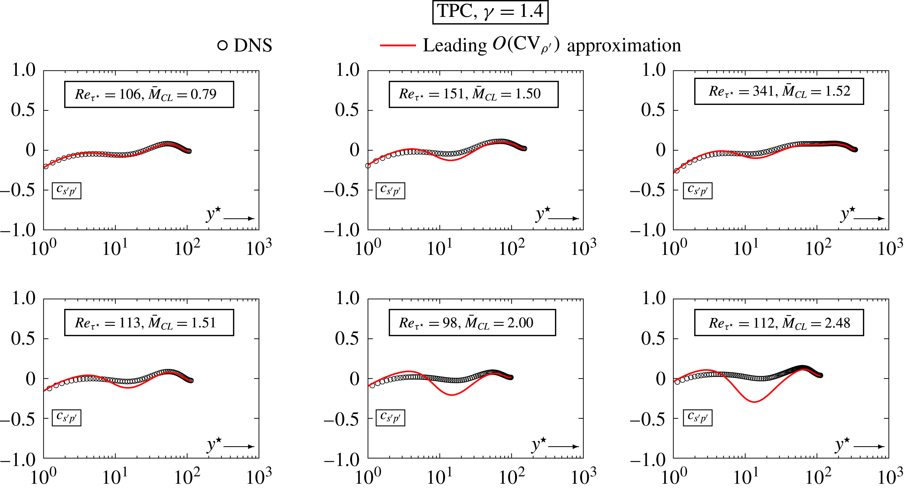
Figure 11. Comparison of the leading
 $O(\text{CV}_{\unicode[STIX]{x1D70C}^{\prime }})$
approximation (4.7c
) of
$O(\text{CV}_{\unicode[STIX]{x1D70C}^{\prime }})$
approximation (4.7c
) of
 $c_{s^{\prime }p^{\prime }}(\text{CV}_{\unicode[STIX]{x1D70C}^{\prime }},\text{CV}_{T^{\prime }},\text{CV}_{p^{\prime }})$
with DNS data for compressible fully developed turbulent plane channel (TPC) flow (Gerolymos & Vallet Reference Gerolymos and Vallet2014), plotted against the HCB-scaled wall distance
$c_{s^{\prime }p^{\prime }}(\text{CV}_{\unicode[STIX]{x1D70C}^{\prime }},\text{CV}_{T^{\prime }},\text{CV}_{p^{\prime }})$
with DNS data for compressible fully developed turbulent plane channel (TPC) flow (Gerolymos & Vallet Reference Gerolymos and Vallet2014), plotted against the HCB-scaled wall distance
 $y^{\star }$
(3.2b,c
), for different values of
$y^{\star }$
(3.2b,c
), for different values of
 $Re_{\unicode[STIX]{x1D70F}^{\star }}\in [98,341]$
and
$Re_{\unicode[STIX]{x1D70F}^{\star }}\in [98,341]$
and
 $\bar{M}_{CL}\in [0.8,2.5]$
.
$\bar{M}_{CL}\in [0.8,2.5]$
.

Figure 12. Comparison of the leading
 $O(\text{CV}_{\unicode[STIX]{x1D70C}^{\prime }})$
approximation (4.3c
) of
$O(\text{CV}_{\unicode[STIX]{x1D70C}^{\prime }})$
approximation (4.3c
) of
 $c_{\unicode[STIX]{x1D70C}^{\prime }T^{\prime }}(\text{CV}_{\unicode[STIX]{x1D70C}^{\prime }},\text{CV}_{T^{\prime }},\text{CV}_{p^{\prime }})$
with sustained homogeneous isotropic turbulence (HIT) DNS data (Donzis & Jagannathan Reference Donzis and Jagannathan2013; D. A. Donzis, 2016, Private communication; Jagannathan & Donzis Reference Jagannathan and Donzis2016), plotted against the turbulent Mach number
$c_{\unicode[STIX]{x1D70C}^{\prime }T^{\prime }}(\text{CV}_{\unicode[STIX]{x1D70C}^{\prime }},\text{CV}_{T^{\prime }},\text{CV}_{p^{\prime }})$
with sustained homogeneous isotropic turbulence (HIT) DNS data (Donzis & Jagannathan Reference Donzis and Jagannathan2013; D. A. Donzis, 2016, Private communication; Jagannathan & Donzis Reference Jagannathan and Donzis2016), plotted against the turbulent Mach number
 $M_{T}\in [0.1,0.6]$
, for different values of
$M_{T}\in [0.1,0.6]$
, for different values of
 $Re_{\unicode[STIX]{x1D706}}\in [35,430]$
(solid symbols: DNS, open symbols: approximation).
$Re_{\unicode[STIX]{x1D706}}\in [35,430]$
(solid symbols: DNS, open symbols: approximation).

Figure 13. Leading-order estimates (4.5a
), (4.3), (4.7) for
 $\{R_{g}^{-1}\,\text{CV}_{\unicode[STIX]{x1D70C}^{\prime }}^{-1}\,s_{rms}^{\prime },c_{p^{\prime }\unicode[STIX]{x1D70C}^{\prime }},c_{p^{\prime }T^{\prime }},c_{\unicode[STIX]{x1D70C}^{\prime }T^{\prime }},c_{s^{\prime }\unicode[STIX]{x1D70C}^{\prime }},c_{s^{\prime }T^{\prime }},c_{s^{\prime }p^{\prime }}\}$
with input DNS data for
$\{R_{g}^{-1}\,\text{CV}_{\unicode[STIX]{x1D70C}^{\prime }}^{-1}\,s_{rms}^{\prime },c_{p^{\prime }\unicode[STIX]{x1D70C}^{\prime }},c_{p^{\prime }T^{\prime }},c_{\unicode[STIX]{x1D70C}^{\prime }T^{\prime }},c_{s^{\prime }\unicode[STIX]{x1D70C}^{\prime }},c_{s^{\prime }T^{\prime }},c_{s^{\prime }p^{\prime }}\}$
with input DNS data for
 $\{\text{CV}_{\unicode[STIX]{x1D70C}^{\prime }},\text{CV}_{T^{\prime }},\text{CV}_{p^{\prime }}\}$
from sustained compressible HIT computations (Donzis & Jagannathan Reference Donzis and Jagannathan2013; D. A. Donzis, 2016, Private communication; Jagannathan & Donzis Reference Jagannathan and Donzis2016), for different values of
$\{\text{CV}_{\unicode[STIX]{x1D70C}^{\prime }},\text{CV}_{T^{\prime }},\text{CV}_{p^{\prime }}\}$
from sustained compressible HIT computations (Donzis & Jagannathan Reference Donzis and Jagannathan2013; D. A. Donzis, 2016, Private communication; Jagannathan & Donzis Reference Jagannathan and Donzis2016), for different values of
 $Re_{\unicode[STIX]{x1D706}}\in [35,430]$
, plotted against the turbulent Mach number
$Re_{\unicode[STIX]{x1D706}}\in [35,430]$
, plotted against the turbulent Mach number
 $M_{T}\in [0.1,0.6]$
.
$M_{T}\in [0.1,0.6]$
.
The approximations (4.5a
), (4.7) are assessed (figures 8–11) against DNS data for compressible channel flow (Gerolymos & Vallet Reference Gerolymos and Vallet2014). These data were obtained by computing the instantaneous entropy field
 $s(\boldsymbol{x},t)$
exactly (Gerolymos & Vallet Reference Gerolymos and Vallet2014, (2.5), p. 710) and sampling (Gerolymos et al.
Reference Gerolymos, Sénéchal and Vallet2010, § 4.4, p. 791) the appropriate moments: they involve no approximation or truncation.
$s(\boldsymbol{x},t)$
exactly (Gerolymos & Vallet Reference Gerolymos and Vallet2014, (2.5), p. 710) and sampling (Gerolymos et al.
Reference Gerolymos, Sénéchal and Vallet2010, § 4.4, p. 791) the appropriate moments: they involve no approximation or truncation.
The leading-order approximations (4.5a
) of
 $R_{g}^{-1}\,s_{rms}^{\prime }$
(figure 8), (4.7a
) of
$R_{g}^{-1}\,s_{rms}^{\prime }$
(figure 8), (4.7a
) of
 $c_{s^{\prime }\unicode[STIX]{x1D70C}^{\prime }}$
(figure 9), and (4.7b
) of
$c_{s^{\prime }\unicode[STIX]{x1D70C}^{\prime }}$
(figure 9), and (4.7b
) of
 $c_{s^{\prime }T^{\prime }}$
(figure 10) are in excellent agreement with DNS data
$c_{s^{\prime }T^{\prime }}$
(figure 10) are in excellent agreement with DNS data
 $\forall \,y^{\star }$
and for every available
$\forall \,y^{\star }$
and for every available
 $(Re_{\unicode[STIX]{x1D70F}^{\star }},\bar{M}_{CL})$
. On the contrary the leading-order approximation (4.7c
) of
$(Re_{\unicode[STIX]{x1D70F}^{\star }},\bar{M}_{CL})$
. On the contrary the leading-order approximation (4.7c
) of
 $c_{s^{\prime }p^{\prime }}$
(figure 11) behaves in a manner similar to the leading-order approximations (4.3a
), (4.3b
) of
$c_{s^{\prime }p^{\prime }}$
(figure 11) behaves in a manner similar to the leading-order approximations (4.3a
), (4.3b
) of
 $c_{p^{\prime }\unicode[STIX]{x1D70C}^{\prime }}$
(figure 6) and of
$c_{p^{\prime }\unicode[STIX]{x1D70C}^{\prime }}$
(figure 6) and of
 $c_{p^{\prime }T^{\prime }}$
(figure 7). It is excellent for
$c_{p^{\prime }T^{\prime }}$
(figure 7). It is excellent for
 $\bar{M}_{CL}\approxeq 0.8$
and satisfactory for
$\bar{M}_{CL}\approxeq 0.8$
and satisfactory for
 $\bar{M}_{CL}\approxeq 1.5$
, but presents discrepancies for the higher
$\bar{M}_{CL}\approxeq 1.5$
, but presents discrepancies for the higher
 $\bar{M}_{CL}\in \{2,2.5\}$
(figure 11), in the range
$\bar{M}_{CL}\in \{2,2.5\}$
(figure 11), in the range
 $10\lessapprox y^{\star }\lessapprox 40$
. Again, the leading error in (4.7c
) involves division by
$10\lessapprox y^{\star }\lessapprox 40$
. Again, the leading error in (4.7c
) involves division by
 $\text{CV}_{p^{\prime }}$
and suffers from the high values of
$\text{CV}_{p^{\prime }}$
and suffers from the high values of
 $\text{CV}_{p^{\prime }}^{-1}\text{CV}_{\unicode[STIX]{x1D70C}^{\prime }}$
and
$\text{CV}_{p^{\prime }}^{-1}\text{CV}_{\unicode[STIX]{x1D70C}^{\prime }}$
and
 $\text{CV}_{p^{\prime }}^{-1}\text{CV}_{T^{\prime }}$
(figure 3).
$\text{CV}_{p^{\prime }}^{-1}\text{CV}_{T^{\prime }}$
(figure 3).
As a conclusion, nonlinear effects of compressibility seem to influence some features of the thermodynamic correlations containing
 $p^{\prime }$
when
$p^{\prime }$
when
 $\bar{M}_{CL}\gtrapprox 2$
(figures 5–7): in this range, the quadratic terms in the exact relations (2.5) cannot be neglected. Nonetheless, the region where these nonlinear compressibility effects are important remains confined in the buffer zone of the wall layer (Smits & Dussauge Reference Smits and Dussauge2006, p. 203).
$\bar{M}_{CL}\gtrapprox 2$
(figures 5–7): in this range, the quadratic terms in the exact relations (2.5) cannot be neglected. Nonetheless, the region where these nonlinear compressibility effects are important remains confined in the buffer zone of the wall layer (Smits & Dussauge Reference Smits and Dussauge2006, p. 203).
5.2 Approximation accuracy in sustained compressible HIT
Only
 $c_{\unicode[STIX]{x1D70C}^{\prime }T^{\prime }}$
was available in the HIT DNS database (Donzis & Jagannathan Reference Donzis and Jagannathan2013; D. A. Donzis, 2016, Private communication; Jagannathan & Donzis Reference Jagannathan and Donzis2016). The leading-order approximation (4.3c
) compares very well with the DNS data (figure 12), corroborating the conclusion (§ 5.1) that (4.3c
) is a very robust approximation. Notice also that the ratios
$c_{\unicode[STIX]{x1D70C}^{\prime }T^{\prime }}$
was available in the HIT DNS database (Donzis & Jagannathan Reference Donzis and Jagannathan2013; D. A. Donzis, 2016, Private communication; Jagannathan & Donzis Reference Jagannathan and Donzis2016). The leading-order approximation (4.3c
) compares very well with the DNS data (figure 12), corroborating the conclusion (§ 5.1) that (4.3c
) is a very robust approximation. Notice also that the ratios
 $\text{CV}_{p^{\prime }}^{-1}\text{CV}_{T^{\prime }}$
and
$\text{CV}_{p^{\prime }}^{-1}\text{CV}_{T^{\prime }}$
and
 $\text{CV}_{p^{\prime }}^{-1}\text{CV}_{\unicode[STIX]{x1D70C}^{\prime }}$
which multiply the leading error of the approximations (4.3a
) for
$\text{CV}_{p^{\prime }}^{-1}\text{CV}_{\unicode[STIX]{x1D70C}^{\prime }}$
which multiply the leading error of the approximations (4.3a
) for
 $c_{p^{\prime }\unicode[STIX]{x1D70C}^{\prime }}$
and (4.3b
) for
$c_{p^{\prime }\unicode[STIX]{x1D70C}^{\prime }}$
and (4.3b
) for
 $c_{p^{\prime }T^{\prime }}$
are invariably
$c_{p^{\prime }T^{\prime }}$
are invariably
 ${<}1$
in HIT (figure 2). Therefore, we expect that the approximations (4.3a
), (4.3b
) of
${<}1$
in HIT (figure 2). Therefore, we expect that the approximations (4.3a
), (4.3b
) of
 $c_{p^{\prime }\unicode[STIX]{x1D70C}^{\prime }}$
and
$c_{p^{\prime }\unicode[STIX]{x1D70C}^{\prime }}$
and
 $c_{p^{\prime }T^{\prime }}$
should be quite accurate for the HIT case. Of course data for these correlations are needed to fully substantiate this conjecture.
$c_{p^{\prime }T^{\prime }}$
should be quite accurate for the HIT case. Of course data for these correlations are needed to fully substantiate this conjecture.
The leading-order approximations (4.3), (4.5a
), (4.7) can be used to discuss the behaviour of compressible HIT, in terms of correlations that were not available in the database (Donzis & Jagannathan Reference Donzis and Jagannathan2013; D. A. Donzis, 2016, Private communication; Jagannathan & Donzis Reference Jagannathan and Donzis2016). At the highest
 $M_{T}\approxeq 0.6$
sustained compressible HIT data (Donzis & Jagannathan Reference Donzis and Jagannathan2013, table 1, p. 225),
$M_{T}\approxeq 0.6$
sustained compressible HIT data (Donzis & Jagannathan Reference Donzis and Jagannathan2013, table 1, p. 225),
 $\text{CV}_{\unicode[STIX]{x1D70C}^{\prime }}\approxeq 0.16$
,
$\text{CV}_{\unicode[STIX]{x1D70C}^{\prime }}\approxeq 0.16$
,
 $\text{CV}_{p^{\prime }}\approxeq 0.22$
and
$\text{CV}_{p^{\prime }}\approxeq 0.22$
and
 $\text{CV}_{T^{\prime }}\approxeq 0.06$
. Based on the assessment of the leading-order approximations (4.3), (4.5a
), (4.7) for compressible channel flow (figures 5–11) we expect these approximations to be reasonably accurate, and use them to investigate the behaviour of compressible HIT with increasing
$\text{CV}_{T^{\prime }}\approxeq 0.06$
. Based on the assessment of the leading-order approximations (4.3), (4.5a
), (4.7) for compressible channel flow (figures 5–11) we expect these approximations to be reasonably accurate, and use them to investigate the behaviour of compressible HIT with increasing
 $M_{T}$
(figure 13). The non-dimensional ratio of entropy and density fluctuations
$M_{T}$
(figure 13). The non-dimensional ratio of entropy and density fluctuations
 $R_{g}^{-1}\text{CV}_{\unicode[STIX]{x1D70C}^{\prime }}^{-1}s_{rms}^{\prime }$
decreases with increasing
$R_{g}^{-1}\text{CV}_{\unicode[STIX]{x1D70C}^{\prime }}^{-1}s_{rms}^{\prime }$
decreases with increasing
 $M_{T}$
and shows significant
$M_{T}$
and shows significant
 $Re_{\unicode[STIX]{x1D706}}$
-dependency (figure 13), which is not surprising since
$Re_{\unicode[STIX]{x1D706}}$
-dependency (figure 13), which is not surprising since
 $s_{rms}^{\prime }$
is largely the result of dissipative phenomena. The various correlation coefficients depend mainly on
$s_{rms}^{\prime }$
is largely the result of dissipative phenomena. The various correlation coefficients depend mainly on
 $M_{T}$
, with a weaker
$M_{T}$
, with a weaker
 $Re_{\unicode[STIX]{x1D706}}$
-dependency (figure 13). We observe in particular that
$Re_{\unicode[STIX]{x1D706}}$
-dependency (figure 13). We observe in particular that
 $c_{s^{\prime }T^{\prime }}\approxeq 0.2\;\forall \;(M_{T},Re_{\unicode[STIX]{x1D706}})$
remains practically constant with little scatter (figure 13). This observation is further confirmed in § 6 and will be used in § 7.1 to suggest a simple model for the thermodynamic turbulence structure of subsonic sustained compressible HIT.
$c_{s^{\prime }T^{\prime }}\approxeq 0.2\;\forall \;(M_{T},Re_{\unicode[STIX]{x1D706}})$
remains practically constant with little scatter (figure 13). This observation is further confirmed in § 6 and will be used in § 7.1 to suggest a simple model for the thermodynamic turbulence structure of subsonic sustained compressible HIT.
6 Compressible aerodynamic turbulence map
The different approximate expressions developed above (4.3), (4.4), (4.5), (4.7) can be used to map the behaviour of compressible turbulence. We will assume in the following the validity of these leading-order approximations. The important and robust relation (4.4) suggests working in the
 $(\text{CV}_{\unicode[STIX]{x1D70C}^{\prime }}^{-1}\text{CV}_{T^{\prime }},c_{\unicode[STIX]{x1D70C}^{\prime }T^{\prime }})$
-plane (figure 14), limited by (2.3a
) to
$(\text{CV}_{\unicode[STIX]{x1D70C}^{\prime }}^{-1}\text{CV}_{T^{\prime }},c_{\unicode[STIX]{x1D70C}^{\prime }T^{\prime }})$
-plane (figure 14), limited by (2.3a
) to
 $-1\leqslant c_{\unicode[STIX]{x1D70C}^{\prime }T^{\prime }}\leqslant +1$
.
$-1\leqslant c_{\unicode[STIX]{x1D70C}^{\prime }T^{\prime }}\leqslant +1$
.

Figure 14. Map for
 $\breve{\unicode[STIX]{x1D6FE}}=1.4$
on the
$\breve{\unicode[STIX]{x1D6FE}}=1.4$
on the
 $(\text{CV}_{\unicode[STIX]{x1D70C}^{\prime }}^{-1}\,\text{CV}_{T^{\prime }},c_{\unicode[STIX]{x1D70C}^{\prime }T^{\prime }})$
-plane of DNS data for compressible solenoidally forced sustained HIT (Donzis & Jagannathan Reference Donzis and Jagannathan2013; D. A. Donzis, 2016, Private communication; Jagannathan & Donzis Reference Jagannathan and Donzis2016,
$(\text{CV}_{\unicode[STIX]{x1D70C}^{\prime }}^{-1}\,\text{CV}_{T^{\prime }},c_{\unicode[STIX]{x1D70C}^{\prime }T^{\prime }})$
-plane of DNS data for compressible solenoidally forced sustained HIT (Donzis & Jagannathan Reference Donzis and Jagannathan2013; D. A. Donzis, 2016, Private communication; Jagannathan & Donzis Reference Jagannathan and Donzis2016,
 $0.1\lessapprox M_{T}\lessapprox 0.6$
,
$0.1\lessapprox M_{T}\lessapprox 0.6$
,
 $35\lessapprox Re_{\unicode[STIX]{x1D706}}\lessapprox 430$
) and for fully developed compressible turbulent plane channel (TPC) flow (Gerolymos & Vallet Reference Gerolymos and Vallet2014,
$35\lessapprox Re_{\unicode[STIX]{x1D706}}\lessapprox 430$
) and for fully developed compressible turbulent plane channel (TPC) flow (Gerolymos & Vallet Reference Gerolymos and Vallet2014,
 $0.35\lessapprox \bar{M}_{CL}\lessapprox 2.48$
,
$0.35\lessapprox \bar{M}_{CL}\lessapprox 2.48$
,
 $78\lessapprox Re_{\unicode[STIX]{x1D70F}^{\star }}\lessapprox 341$
), approximate (to leading order) loci of
$78\lessapprox Re_{\unicode[STIX]{x1D70F}^{\star }}\lessapprox 341$
), approximate (to leading order) loci of
 $[c_{s^{\prime }p^{\prime }}=0]$
(6.4), of
$[c_{s^{\prime }p^{\prime }}=0]$
(6.4), of
 $[c_{s^{\prime }T^{\prime }}=0.2]$
(6.2) and of
$[c_{s^{\prime }T^{\prime }}=0.2]$
(6.2) and of
 $[c_{p^{\prime }T^{\prime }}=0.1]$
(6.3), describing turbulence structure of specific flow regions, various zones (I to V;
$[c_{p^{\prime }T^{\prime }}=0.1]$
(6.3), describing turbulence structure of specific flow regions, various zones (I to V;
 $\breve{\unicode[STIX]{x1D6FE}}=1.4$
) corresponding to different orderings of the non-dimensional
$\breve{\unicode[STIX]{x1D6FE}}=1.4$
) corresponding to different orderings of the non-dimensional
 $\text{r.m.s.}$
levels of thermodynamic fluctuations, and isolated point (within the leading-order approximate framework) of isentropic turbulence (6.1).
$\text{r.m.s.}$
levels of thermodynamic fluctuations, and isolated point (within the leading-order approximate framework) of isentropic turbulence (6.1).
The abscissa
 $\text{CV}_{\unicode[STIX]{x1D70C}^{\prime }}^{-1}\,\text{CV}_{T^{\prime }}$
separates (figure 14) the region
$\text{CV}_{\unicode[STIX]{x1D70C}^{\prime }}^{-1}\,\text{CV}_{T^{\prime }}$
separates (figure 14) the region
 $\text{CV}_{\unicode[STIX]{x1D70C}^{\prime }}>\text{CV}_{T^{\prime }}$
from the region
$\text{CV}_{\unicode[STIX]{x1D70C}^{\prime }}>\text{CV}_{T^{\prime }}$
from the region
 $\text{CV}_{\unicode[STIX]{x1D70C}^{\prime }}<\text{CV}_{T^{\prime }}$
. Most of the DNS data considered in the paper (§ 3) satisfy
$\text{CV}_{\unicode[STIX]{x1D70C}^{\prime }}<\text{CV}_{T^{\prime }}$
. Most of the DNS data considered in the paper (§ 3) satisfy
 $\text{CV}_{T^{\prime }}<\text{CV}_{\unicode[STIX]{x1D70C}^{\prime }}$
, except for a few near-wall channel data (figure 14), roughly corresponding to the peaks of
$\text{CV}_{T^{\prime }}<\text{CV}_{\unicode[STIX]{x1D70C}^{\prime }}$
, except for a few near-wall channel data (figure 14), roughly corresponding to the peaks of
 $\text{CV}_{\unicode[STIX]{x1D70C}^{\prime }}$
and
$\text{CV}_{\unicode[STIX]{x1D70C}^{\prime }}$
and
 $\text{CV}_{T^{\prime }}$
(Gerolymos & Vallet Reference Gerolymos and Vallet2014, figure 5, p. 720) around
$\text{CV}_{T^{\prime }}$
(Gerolymos & Vallet Reference Gerolymos and Vallet2014, figure 5, p. 720) around
 $y^{\star }\approxeq 7$
where values
$y^{\star }\approxeq 7$
where values
 $\text{CV}_{\unicode[STIX]{x1D70C}^{\prime }}\approxeq \text{CV}_{T^{\prime }}$
are observed (figure 14). Simple calculations define zones on the
$\text{CV}_{\unicode[STIX]{x1D70C}^{\prime }}\approxeq \text{CV}_{T^{\prime }}$
are observed (figure 14). Simple calculations define zones on the
 $(\text{CV}_{\unicode[STIX]{x1D70C}^{\prime }}^{-1}\,\text{CV}_{T^{\prime }},c_{\unicode[STIX]{x1D70C}^{\prime }T^{\prime }})$
-plane (figure 14) with specific orderings of the non-dimensional
$(\text{CV}_{\unicode[STIX]{x1D70C}^{\prime }}^{-1}\,\text{CV}_{T^{\prime }},c_{\unicode[STIX]{x1D70C}^{\prime }T^{\prime }})$
-plane (figure 14) with specific orderings of the non-dimensional
 $\text{r.m.s.}$
levels of thermodynamic fluctuations
$\text{r.m.s.}$
levels of thermodynamic fluctuations
 $\{\text{CV}_{p^{\prime }},\text{CV}_{\unicode[STIX]{x1D70C}^{\prime }},\text{CV}_{T^{\prime }},R_{g}^{-1}\,s_{rms}^{\prime }\}$
. For simplicity we study the case
$\{\text{CV}_{p^{\prime }},\text{CV}_{\unicode[STIX]{x1D70C}^{\prime }},\text{CV}_{T^{\prime }},R_{g}^{-1}\,s_{rms}^{\prime }\}$
. For simplicity we study the case
 $\breve{\unicode[STIX]{x1D6FE}}=1.4$
. Zone I at the bottom (figure 14), is characterized by low
$\breve{\unicode[STIX]{x1D6FE}}=1.4$
. Zone I at the bottom (figure 14), is characterized by low
 $\text{CV}_{p^{\prime }}$
compared to
$\text{CV}_{p^{\prime }}$
compared to
 $\text{CV}_{\unicode[STIX]{x1D70C}^{\prime }}$
and
$\text{CV}_{\unicode[STIX]{x1D70C}^{\prime }}$
and
 $\text{CV}_{T^{\prime }}$
, contrary to the four other zones, which are essentially distinguished with respect to the relative importance of the non-dimensional entropy fluctuations. In zone I,
$\text{CV}_{T^{\prime }}$
, contrary to the four other zones, which are essentially distinguished with respect to the relative importance of the non-dimensional entropy fluctuations. In zone I,
 $R_{g}^{-1}\,s_{rms}^{\prime }$
is higher than
$R_{g}^{-1}\,s_{rms}^{\prime }$
is higher than
 $\{\text{CV}_{\unicode[STIX]{x1D70C}^{\prime }},\text{CV}_{T^{\prime }},\text{CV}_{p^{\prime }}\}$
, progressively diminishing through zones I–V. Zone V, where
$\{\text{CV}_{\unicode[STIX]{x1D70C}^{\prime }},\text{CV}_{T^{\prime }},\text{CV}_{p^{\prime }}\}$
, progressively diminishing through zones I–V. Zone V, where
 $R_{g}^{-1}\,s_{rms}^{\prime }\lessapprox \text{CV}_{T^{\prime }}\lessapprox \text{CV}_{\unicode[STIX]{x1D70C}^{\prime }}\lessapprox \text{CV}_{p^{\prime }}$
(figure 14), also contains the isolated point of isentropic turbulence, where
$R_{g}^{-1}\,s_{rms}^{\prime }\lessapprox \text{CV}_{T^{\prime }}\lessapprox \text{CV}_{\unicode[STIX]{x1D70C}^{\prime }}\lessapprox \text{CV}_{p^{\prime }}$
(figure 14), also contains the isolated point of isentropic turbulence, where
 $$\begin{eqnarray}\displaystyle \Big[s_{rms}^{\prime }=0\stackrel{\text{(2.1a)}}{\;\Longleftrightarrow \;}s^{\prime }=0\,\forall \,t\Big]\stackrel{\text{(4.5b)},\,\text{(4.4)}}{\;\Longleftrightarrow \;}\left\{\begin{array}{@{}l@{}}c_{\unicode[STIX]{x1D70C}^{\prime }T^{\prime }}\approxeq +1\\ \text{CV}_{T^{\prime }}\approxeq (\breve{\unicode[STIX]{x1D6FE}}-1)\,\text{CV}_{\unicode[STIX]{x1D70C}^{\prime }}\\ \text{CV}_{p^{\prime }}\approxeq \breve{\unicode[STIX]{x1D6FE}}\,\text{CV}_{\unicode[STIX]{x1D70C}^{\prime }}.\end{array}\right. & & \displaystyle\end{eqnarray}$$
Of course this is an inaccessible limit point, since it is highly improbable (impossible) for a turbulent flow to have
 $s^{\prime }=0\,\forall \,t$
. Available DNS data for
$s^{\prime }=0\,\forall \,t$
. Available DNS data for
 $\{\text{CV}_{\unicode[STIX]{x1D70C}^{\prime }}^{-1}\,\text{CV}_{T^{\prime }},c_{\unicode[STIX]{x1D70C}^{\prime }T^{\prime }}\}$
(Donzis & Jagannathan Reference Donzis and Jagannathan2013; Gerolymos & Vallet Reference Gerolymos and Vallet2014; D. A. Donzis, 2016, Private communication; Jagannathan & Donzis Reference Jagannathan and Donzis2016) show that different flows or flow regions have specific thermodynamic turbulence structure (figure 14).
$\{\text{CV}_{\unicode[STIX]{x1D70C}^{\prime }}^{-1}\,\text{CV}_{T^{\prime }},c_{\unicode[STIX]{x1D70C}^{\prime }T^{\prime }}\}$
(Donzis & Jagannathan Reference Donzis and Jagannathan2013; Gerolymos & Vallet Reference Gerolymos and Vallet2014; D. A. Donzis, 2016, Private communication; Jagannathan & Donzis Reference Jagannathan and Donzis2016) show that different flows or flow regions have specific thermodynamic turbulence structure (figure 14).
As already observed (figure 13) the HIT data follow (for the available
 $\unicode[STIX]{x1D6FE}=1.4$
computations) the
$\unicode[STIX]{x1D6FE}=1.4$
computations) the
 $[c_{s^{\prime }T^{\prime }}\approxeq 0.2]$
-line, which is easily calculated as
$[c_{s^{\prime }T^{\prime }}\approxeq 0.2]$
-line, which is easily calculated as
 $$\begin{eqnarray}\displaystyle c_{\unicode[STIX]{x1D70C}^{\prime }T^{\prime }}\stackrel{\text{(4.5b)},\,\text{(4.6b)}}{\approxeq }\left[{\displaystyle \frac{1-c_{s^{\prime }T^{\prime }}^{2}}{\breve{\unicode[STIX]{x1D6FE}}-1}}\,{\displaystyle \frac{\text{CV}_{T^{\prime }}}{\text{CV}_{\unicode[STIX]{x1D70C}^{\prime }}}}\pm c_{s^{\prime }T^{\prime }}\sqrt{1-{\displaystyle \frac{1-c_{s^{\prime }T^{\prime }}^{2}}{(\breve{\unicode[STIX]{x1D6FE}}-1)^{2}}}\,\left({\displaystyle \frac{\text{CV}_{T^{\prime }}}{\text{CV}_{\unicode[STIX]{x1D70C}^{\prime }}}}\right)^{2}}\right]_{\left(c_{s^{\prime }T^{\prime }}=0.2,\breve{\unicode[STIX]{x1D6FE}}=1.4\right)}. & & \displaystyle\end{eqnarray}$$
There is little scatter in the HIT DNS data (figure 14) except for one outlier corresponding to the
 $(Re_{\unicode[STIX]{x1D706}},M_{T})\approxeq (60,0.1)$
simulation (Donzis & Jagannathan Reference Donzis and Jagannathan2013, table 1, p. 225). Mapping on the
$(Re_{\unicode[STIX]{x1D706}},M_{T})\approxeq (60,0.1)$
simulation (Donzis & Jagannathan Reference Donzis and Jagannathan2013, table 1, p. 225). Mapping on the
 $(\text{CV}_{\unicode[STIX]{x1D70C}^{\prime }}^{-1}\,\text{CV}_{T^{\prime }},c_{\unicode[STIX]{x1D70C}^{\prime }T^{\prime }})$
-plane explains why the alternative observation (figure 13) that the HIT data are also quite close to
$(\text{CV}_{\unicode[STIX]{x1D70C}^{\prime }}^{-1}\,\text{CV}_{T^{\prime }},c_{\unicode[STIX]{x1D70C}^{\prime }T^{\prime }})$
-plane explains why the alternative observation (figure 13) that the HIT data are also quite close to
 $c_{p^{\prime }\unicode[STIX]{x1D70C}^{\prime }}\approxeq 1$
cannot be used, as it would erroneously imply by (4.3a
), (4.4)
$c_{p^{\prime }\unicode[STIX]{x1D70C}^{\prime }}\approxeq 1$
cannot be used, as it would erroneously imply by (4.3a
), (4.4)
 $c_{\unicode[STIX]{x1D70C}^{\prime }T^{\prime }}\approxeq 1$
: in general approximations based on
$c_{\unicode[STIX]{x1D70C}^{\prime }T^{\prime }}\approxeq 1$
: in general approximations based on
 $\pm 1$
values of correlation coefficients are singular as they invariably map by (4.3), (4.5), (4.6) to
$\pm 1$
values of correlation coefficients are singular as they invariably map by (4.3), (4.5), (4.6) to
 $\left|c_{\unicode[STIX]{x1D70C}^{\prime }T^{\prime }}\right|\approxeq 1$
.
$\left|c_{\unicode[STIX]{x1D70C}^{\prime }T^{\prime }}\right|\approxeq 1$
.
The locus of the channel data depends on the non-dimensional wall distance
 $y^{\star }$
(3.2b,c
). The near-wall points
$y^{\star }$
(3.2b,c
). The near-wall points
 $y^{\star }\lessapprox 7$
seem to collapse onto a single curve. Observation of the correlation coefficients plotted against
$y^{\star }\lessapprox 7$
seem to collapse onto a single curve. Observation of the correlation coefficients plotted against
 $y^{\star }$
suggests (figure 7) that in this region
$y^{\star }$
suggests (figure 7) that in this region
 $c_{p^{\prime }T^{\prime }}\approxeq 0.1$
(for the available
$c_{p^{\prime }T^{\prime }}\approxeq 0.1$
(for the available
 $\unicode[STIX]{x1D6FE}=1.4$
computations)
$\unicode[STIX]{x1D6FE}=1.4$
computations)
 $\forall \,(Re_{\unicode[STIX]{x1D70F}^{\star }},\bar{M}_{CL})$
. The appropriate branch of the
$\forall \,(Re_{\unicode[STIX]{x1D70F}^{\star }},\bar{M}_{CL})$
. The appropriate branch of the
 $[c_{p^{\prime }T^{\prime }}\approxeq 0.1]$
-line is determined by
$[c_{p^{\prime }T^{\prime }}\approxeq 0.1]$
-line is determined by
 $$\begin{eqnarray}\displaystyle c_{\unicode[STIX]{x1D70C}^{\prime }T^{\prime }}\stackrel{\text{(4.3b)},\,\text{(4.4)}}{\approxeq }\left[-(1-c_{p^{\prime }T^{\prime }}^{2})\,{\displaystyle \frac{\text{CV}_{T^{\prime }}}{\text{CV}_{\unicode[STIX]{x1D70C}^{\prime }}}}+c_{p^{\prime }T^{\prime }}\sqrt{1-(1-c_{p^{\prime }T^{\prime }}^{2})\,\left({\displaystyle \frac{\text{CV}_{T^{\prime }}}{\text{CV}_{\unicode[STIX]{x1D70C}^{\prime }}}}\right)^{2}}\right]_{\left(c_{p^{\prime }T^{\prime }}=0.1,\breve{\unicode[STIX]{x1D6FE}}=1.4\right)}.\quad & & \displaystyle\end{eqnarray}$$
Although the mapping relation (6.3) does not involve
 $\breve{\unicode[STIX]{x1D6FE}}$
, it should be kept in mind that the observed value (
$\breve{\unicode[STIX]{x1D6FE}}$
, it should be kept in mind that the observed value (
 $c_{p^{\prime }T^{\prime }}\approxeq 0.1$
) was obtained from
$c_{p^{\prime }T^{\prime }}\approxeq 0.1$
) was obtained from
 $[\unicode[STIX]{x1D6FE}=1.4]$
-computations, and also that the wall is isothermal and cold with respect to the flow (Gerolymos & Vallet Reference Gerolymos and Vallet2014, figure 1, p. 713). All available near-wall (
$[\unicode[STIX]{x1D6FE}=1.4]$
-computations, and also that the wall is isothermal and cold with respect to the flow (Gerolymos & Vallet Reference Gerolymos and Vallet2014, figure 1, p. 713). All available near-wall (
 $y^{\star }\lessapprox 7$
) data follow the
$y^{\star }\lessapprox 7$
) data follow the
 $[c_{p^{\prime }T^{\prime }}\approxeq 0.1]$
-line with little scatter (figure 14).
$[c_{p^{\prime }T^{\prime }}\approxeq 0.1]$
-line with little scatter (figure 14).
In the region
 $7\lessapprox y^{\star }\lessapprox 30$
, roughly the lower buffer layer (Smits & Dussauge Reference Smits and Dussauge2006, p. 203), suggests (figure 11) that
$7\lessapprox y^{\star }\lessapprox 30$
, roughly the lower buffer layer (Smits & Dussauge Reference Smits and Dussauge2006, p. 203), suggests (figure 11) that
 $c_{s^{\prime }p^{\prime }}\approxeq 0$
(for the available
$c_{s^{\prime }p^{\prime }}\approxeq 0$
(for the available
 $\unicode[STIX]{x1D6FE}=1.4$
computations),
$\unicode[STIX]{x1D6FE}=1.4$
computations),
 $\forall \,(Re_{\unicode[STIX]{x1D70F}^{\star }},\bar{M}_{CL})$
. Plotting the
$\forall \,(Re_{\unicode[STIX]{x1D70F}^{\star }},\bar{M}_{CL})$
. Plotting the
 $[c_{s^{\prime }p^{\prime }}\approxeq 0]$
-line, which is determined by
$[c_{s^{\prime }p^{\prime }}\approxeq 0]$
-line, which is determined by
 $$\begin{eqnarray}\displaystyle c_{\unicode[STIX]{x1D70C}^{\prime }T^{\prime }}\stackrel{\text{(A2b)},\,\text{(4.5b)}}{\approxeq }\left[{\displaystyle \frac{\breve{\unicode[STIX]{x1D6FE}}-1}{2-\breve{\unicode[STIX]{x1D6FE}}}}{\displaystyle \frac{\text{CV}_{\unicode[STIX]{x1D70C}^{\prime }}}{\text{CV}_{T^{\prime }}}}-{\displaystyle \frac{1}{2-\breve{\unicode[STIX]{x1D6FE}}}}{\displaystyle \frac{\text{CV}_{T^{\prime }}}{\text{CV}_{\unicode[STIX]{x1D70C}^{\prime }}}}\right]_{\left(c_{s^{\prime }p^{\prime }}=0,\breve{\unicode[STIX]{x1D6FE}}=1.4\right)} & & \displaystyle\end{eqnarray}$$
indicates good correlation of the data (figure 14). Notice that the data around
 $y^{\star }\approxeq 7$
correspond to a region around the point
$y^{\star }\approxeq 7$
correspond to a region around the point
 $[\text{CV}_{\unicode[STIX]{x1D70C}^{\prime }}=\text{CV}_{T^{\prime }},c_{\unicode[STIX]{x1D70C}^{\prime }T^{\prime }}=-1]$
where the
$[\text{CV}_{\unicode[STIX]{x1D70C}^{\prime }}=\text{CV}_{T^{\prime }},c_{\unicode[STIX]{x1D70C}^{\prime }T^{\prime }}=-1]$
where the
 $[c_{p^{\prime }T^{\prime }}\approxeq 0.1]$
-line (6.3) crosses the
$[c_{p^{\prime }T^{\prime }}\approxeq 0.1]$
-line (6.3) crosses the
 $[c_{s^{\prime }p^{\prime }}\approxeq 0]$
-line (6.4), both fitting the DNS data there (figure 14). DNS data for
$[c_{s^{\prime }p^{\prime }}\approxeq 0]$
-line (6.4), both fitting the DNS data there (figure 14). DNS data for
 $y^{\star }\gtrapprox 30$
stay close (but not on) the
$y^{\star }\gtrapprox 30$
stay close (but not on) the
 $[c_{s^{\prime }p^{\prime }}\approxeq 0]$
-line, and return to this locus near the centreline (figure 14), in line with the detailed plots of
$[c_{s^{\prime }p^{\prime }}\approxeq 0]$
-line, and return to this locus near the centreline (figure 14), in line with the detailed plots of
 $c_{s^{\prime }p^{\prime }}$
versus
$c_{s^{\prime }p^{\prime }}$
versus
 $y^{\star }$
(figure 11).
$y^{\star }$
(figure 11).
The
 $(\text{CV}_{\unicode[STIX]{x1D70C}^{\prime }}^{-1}\text{CV}_{T^{\prime }},c_{\unicode[STIX]{x1D70C}^{\prime }T^{\prime }})$
-plane, essentially inspired by (4.4) is not the only possible choice. The observation e.g. that sustained subsonic compressible HIT evolves with varying
$(\text{CV}_{\unicode[STIX]{x1D70C}^{\prime }}^{-1}\text{CV}_{T^{\prime }},c_{\unicode[STIX]{x1D70C}^{\prime }T^{\prime }})$
-plane, essentially inspired by (4.4) is not the only possible choice. The observation e.g. that sustained subsonic compressible HIT evolves with varying
 $(M_{T},Re_{\unicode[STIX]{x1D706}})$
along a
$(M_{T},Re_{\unicode[STIX]{x1D706}})$
along a
 $[c_{s^{\prime }T^{\prime }}\approxeq \text{const.}]$
-line, and the corresponding model developed in § 7.1, suggest that mapping on the
$[c_{s^{\prime }T^{\prime }}\approxeq \text{const.}]$
-line, and the corresponding model developed in § 7.1, suggest that mapping on the
 $(R_{g}^{-1}\text{CV}_{\unicode[STIX]{x1D70C}^{\prime }}^{-1}s_{rms}^{\prime },c_{s^{\prime }T})$
is an alternative choice. In general, any couple of parameters in the set TTS (1.2) can potentially be used to define the mapping plane: by (4.3), (4.4), (4.5), (4.7) the set TTS (1.2) has, to leading order, 2 degrees-of-freedom.
$(R_{g}^{-1}\text{CV}_{\unicode[STIX]{x1D70C}^{\prime }}^{-1}s_{rms}^{\prime },c_{s^{\prime }T})$
is an alternative choice. In general, any couple of parameters in the set TTS (1.2) can potentially be used to define the mapping plane: by (4.3), (4.4), (4.5), (4.7) the set TTS (1.2) has, to leading order, 2 degrees-of-freedom.
7 Applications
The representations of compressible turbulence in the
 $(\text{CV}_{\unicode[STIX]{x1D70C}^{\prime }}^{-1}\,\text{CV}_{T^{\prime }},c_{\unicode[STIX]{x1D70C}^{\prime }T^{\prime }})$
-plane (CT-map) were found very useful in identifying the behaviour of the thermodynamic fluctuations and of their correlations for different flows or different flow regions (figure 14). Examples of applications are the development of a simple model for thermodynamic turbulence structure of sustained compressible HIT (§ 7.1) and the
$(\text{CV}_{\unicode[STIX]{x1D70C}^{\prime }}^{-1}\,\text{CV}_{T^{\prime }},c_{\unicode[STIX]{x1D70C}^{\prime }T^{\prime }})$
-plane (CT-map) were found very useful in identifying the behaviour of the thermodynamic fluctuations and of their correlations for different flows or different flow regions (figure 14). Examples of applications are the development of a simple model for thermodynamic turbulence structure of sustained compressible HIT (§ 7.1) and the
 $[c_{s^{\prime }p^{\prime }}\approxeq 0]$
-approximation in the lower buffer region (
$[c_{s^{\prime }p^{\prime }}\approxeq 0]$
-approximation in the lower buffer region (
 $7\lessapprox y^{\star }\lessapprox 40$
) in compressible wall turbulence (§ 7.2).
$7\lessapprox y^{\star }\lessapprox 40$
) in compressible wall turbulence (§ 7.2).

Figure 15. Zoom on the
 $(\text{CV}_{\unicode[STIX]{x1D70C}^{\prime }}^{-1}\,\text{CV}_{T^{\prime }},c_{\unicode[STIX]{x1D70C}^{\prime }T^{\prime }})$
-plane of DNS data for compressible solenoidally forced sustained HIT (Donzis & Jagannathan Reference Donzis and Jagannathan2013; D. A. Donzis, 2016, Private communication; Jagannathan & Donzis Reference Jagannathan and Donzis2016,
$(\text{CV}_{\unicode[STIX]{x1D70C}^{\prime }}^{-1}\,\text{CV}_{T^{\prime }},c_{\unicode[STIX]{x1D70C}^{\prime }T^{\prime }})$
-plane of DNS data for compressible solenoidally forced sustained HIT (Donzis & Jagannathan Reference Donzis and Jagannathan2013; D. A. Donzis, 2016, Private communication; Jagannathan & Donzis Reference Jagannathan and Donzis2016,
 $0.1\approxeq M_{T}\approxeq 0.6$
,
$0.1\approxeq M_{T}\approxeq 0.6$
,
 $35\approxeq Re_{\unicode[STIX]{x1D706}}\approxeq 430$
) following the approximation (to leading order) of the
$35\approxeq Re_{\unicode[STIX]{x1D706}}\approxeq 430$
) following the approximation (to leading order) of the
 $[c_{s^{\prime }T^{\prime }}=0.2]$
-locus (6.2), which intersects the
$[c_{s^{\prime }T^{\prime }}=0.2]$
-locus (6.2), which intersects the
 $[c_{s^{\prime }T^{\prime }}=0]$
-locus (6.4) at point
$[c_{s^{\prime }T^{\prime }}=0]$
-locus (6.4) at point
 $Q_{1}$
and the
$Q_{1}$
and the
 $[c_{s^{\prime }\unicode[STIX]{x1D70C}^{\prime }}=0]$
-locus at point
$[c_{s^{\prime }\unicode[STIX]{x1D70C}^{\prime }}=0]$
-locus at point
 $Q_{2}$
, and finally passes through the isolated limit point (within the leading-order approximate framework) of isentropic turbulence (6.1).
$Q_{2}$
, and finally passes through the isolated limit point (within the leading-order approximate framework) of isentropic turbulence (6.1).
7.1 Thermodynamic turbulence structure in sustained subsonic HIT
It appears from DNS data (Donzis & Jagannathan Reference Donzis and Jagannathan2013; D. A. Donzis, 2016, Private communication; Jagannathan & Donzis Reference Jagannathan and Donzis2016) that, as
 $M_{T}$
increases, compressible subsonic HIT thermodynamic turbulence structure parameters (1.2) tend to a slowly varying state (figures 2, 12, 8, 13) with a
$M_{T}$
increases, compressible subsonic HIT thermodynamic turbulence structure parameters (1.2) tend to a slowly varying state (figures 2, 12, 8, 13) with a
 $Re_{\unicode[STIX]{x1D706}}$
-dependency, which is clearly visible e.g. in the evolution of
$Re_{\unicode[STIX]{x1D706}}$
-dependency, which is clearly visible e.g. in the evolution of
 $c_{\unicode[STIX]{x1D70C}^{\prime }T^{\prime }}$
versus
$c_{\unicode[STIX]{x1D70C}^{\prime }T^{\prime }}$
versus
 $M_{T}$
(figure 12) and even more so for
$M_{T}$
(figure 12) and even more so for
 $R_{g}^{-1}\,\text{CV}_{\unicode[STIX]{x1D70C}^{\prime }}^{-1}\,s_{rms}^{\prime }$
versus
$R_{g}^{-1}\,\text{CV}_{\unicode[STIX]{x1D70C}^{\prime }}^{-1}\,s_{rms}^{\prime }$
versus
 $M_{T}$
(figure 13). However, when considering relations between elements of the set TTS (1.2) only, such as mapping on the
$M_{T}$
(figure 13). However, when considering relations between elements of the set TTS (1.2) only, such as mapping on the
 $(\text{CV}_{\unicode[STIX]{x1D70C}^{\prime }}^{-1}\,\text{CV}_{T^{\prime }},c_{\unicode[STIX]{x1D70C}^{\prime }T^{\prime }})$
-plane (figure 14), the DNS data collapse with little scatter on a single curve, following the
$(\text{CV}_{\unicode[STIX]{x1D70C}^{\prime }}^{-1}\,\text{CV}_{T^{\prime }},c_{\unicode[STIX]{x1D70C}^{\prime }T^{\prime }})$
-plane (figure 14), the DNS data collapse with little scatter on a single curve, following the
 $[c_{s^{\prime }T^{\prime }}=0.2]$
-locus (6.2), this value corresponding to the available
$[c_{s^{\prime }T^{\prime }}=0.2]$
-locus (6.2), this value corresponding to the available
 $\unicode[STIX]{x1D6FE}=1.4$
DNS data (Donzis & Jagannathan Reference Donzis and Jagannathan2013; D. A. Donzis, 2016, Private communication; Jagannathan & Donzis Reference Jagannathan and Donzis2016). Zoom on the HIT data in the
$\unicode[STIX]{x1D6FE}=1.4$
DNS data (Donzis & Jagannathan Reference Donzis and Jagannathan2013; D. A. Donzis, 2016, Private communication; Jagannathan & Donzis Reference Jagannathan and Donzis2016). Zoom on the HIT data in the
 $(\text{CV}_{\unicode[STIX]{x1D70C}^{\prime }}^{-1}\,\text{CV}_{T^{\prime }},c_{\unicode[STIX]{x1D70C}^{\prime }T^{\prime }})$
-plane (figure 15) confirms that there is little scatter. The DNS data follow the
$(\text{CV}_{\unicode[STIX]{x1D70C}^{\prime }}^{-1}\,\text{CV}_{T^{\prime }},c_{\unicode[STIX]{x1D70C}^{\prime }T^{\prime }})$
-plane (figure 15) confirms that there is little scatter. The DNS data follow the
 $[c_{s^{\prime }T^{\prime }}=0.2]$
-line (6.2) up to, approximately, its intersection with the
$[c_{s^{\prime }T^{\prime }}=0.2]$
-line (6.2) up to, approximately, its intersection with the
 $[R_{g}^{-1}\,s_{rms}^{\prime }=\text{CV}_{T^{\prime }}]$
-locus which defines the boundary between zones IV and V. The
$[R_{g}^{-1}\,s_{rms}^{\prime }=\text{CV}_{T^{\prime }}]$
-locus which defines the boundary between zones IV and V. The  $[c_{s^{\prime }T^{\prime }}=0.2]$
-line (6.2) terminates (figure 15) at point
$[c_{s^{\prime }T^{\prime }}=0.2]$
-line (6.2) terminates (figure 15) at point
 $Q_{2}$
where
$Q_{2}$
where
 $c_{s^{\prime }\unicode[STIX]{x1D70C}^{\prime }}=0$
. It is then continued (figure 15) by the
$c_{s^{\prime }\unicode[STIX]{x1D70C}^{\prime }}=0$
. It is then continued (figure 15) by the  $[c_{s^{\prime }T^{\prime }}=0.2]$
-line (6.2), which passes through the
$[c_{s^{\prime }T^{\prime }}=0.2]$
-line (6.2), which passes through the
 $[s_{rms}^{\prime }=0]$
-point (6.1). Increasing
$[s_{rms}^{\prime }=0]$
-point (6.1). Increasing
 $M_{T}$
corresponds to decreasing
$M_{T}$
corresponds to decreasing
 $R_{g}^{-1}\,s_{rms}^{\prime }$
(figure 13), i.e. increasing
$R_{g}^{-1}\,s_{rms}^{\prime }$
(figure 13), i.e. increasing
 $c_{\unicode[STIX]{x1D70C}^{\prime }T^{\prime }}$
along the
$c_{\unicode[STIX]{x1D70C}^{\prime }T^{\prime }}$
along the
 $[c_{s^{\prime }T^{\prime }}=0.2]$
-line. Before reaching point
$[c_{s^{\prime }T^{\prime }}=0.2]$
-line. Before reaching point
 $Q_{2}$
, the
$Q_{2}$
, the
 $[c_{s^{\prime }T^{\prime }}=0.2]$
-line intersects (figure 15) the
$[c_{s^{\prime }T^{\prime }}=0.2]$
-line intersects (figure 15) the
 $[c_{s^{\prime }p^{\prime }}=0]$
-line (6.4) at point
$[c_{s^{\prime }p^{\prime }}=0]$
-line (6.4) at point
 $Q_{1}$
. It is unclear how the evolution of HIT continues with increasing
$Q_{1}$
. It is unclear how the evolution of HIT continues with increasing
 $M_{T}$
, since we expect that shocklets and shocks for supersonic
$M_{T}$
, since we expect that shocklets and shocks for supersonic
 $M_{T}>1$
(Wang et al.
Reference Wang, Shi, Wang and He2011) will increase entropy production and substantially modify the thermodynamic turbulence structure (1.2). DNS data for higher
$M_{T}>1$
(Wang et al.
Reference Wang, Shi, Wang and He2011) will increase entropy production and substantially modify the thermodynamic turbulence structure (1.2). DNS data for higher
 $M_{T}$
are required to resolve this issue. We concentrate here on subsonic
$M_{T}$
are required to resolve this issue. We concentrate here on subsonic
 $M_{T}<1$
HIT (Donzis & Jagannathan Reference Donzis and Jagannathan2013; D. A. Donzis, 2016, Private communication; Jagannathan & Donzis Reference Jagannathan and Donzis2016).
$M_{T}<1$
HIT (Donzis & Jagannathan Reference Donzis and Jagannathan2013; D. A. Donzis, 2016, Private communication; Jagannathan & Donzis Reference Jagannathan and Donzis2016). We defer for the moment the quest of a
 $(Re_{\unicode[STIX]{x1D706}},M_{T})$
-correlation of the data and concentrate instead on thermodynamic fluctuations. The data on the
$(Re_{\unicode[STIX]{x1D706}},M_{T})$
-correlation of the data and concentrate instead on thermodynamic fluctuations. The data on the
 $(\text{CV}_{\unicode[STIX]{x1D70C}^{\prime }}^{-1}\,\text{CV}_{T^{\prime }},c_{\unicode[STIX]{x1D70C}^{\prime }T^{\prime }})$
-plane, along the
$(\text{CV}_{\unicode[STIX]{x1D70C}^{\prime }}^{-1}\,\text{CV}_{T^{\prime }},c_{\unicode[STIX]{x1D70C}^{\prime }T^{\prime }})$
-plane, along the
 $[c_{s^{\prime }T^{\prime }}=0.2]$
-line (figures 14, 15) show that
$[c_{s^{\prime }T^{\prime }}=0.2]$
-line (figures 14, 15) show that
 $\text{CV}_{\unicode[STIX]{x1D70C}^{\prime }}^{-1}\,\text{CV}_{T^{\prime }}$
varies little with
$\text{CV}_{\unicode[STIX]{x1D70C}^{\prime }}^{-1}\,\text{CV}_{T^{\prime }}$
varies little with
 $M_{T}$
, contrary to
$M_{T}$
, contrary to
 $R_{g}^{-1}\,\text{CV}_{\unicode[STIX]{x1D70C}^{\prime }}^{-1}\,s_{rms}^{\prime }$
(figure 13). Therefore,
$R_{g}^{-1}\,\text{CV}_{\unicode[STIX]{x1D70C}^{\prime }}^{-1}\,s_{rms}^{\prime }$
(figure 13). Therefore,
 $R_{g}^{-1}\,\text{CV}_{\unicode[STIX]{x1D70C}^{\prime }}^{-1}\,s_{rms}^{\prime }$
is an appropriate structure parameter to be used as independent variable in describing thermodynamic turbulence (1.2), along with the constraint that
$R_{g}^{-1}\,\text{CV}_{\unicode[STIX]{x1D70C}^{\prime }}^{-1}\,s_{rms}^{\prime }$
is an appropriate structure parameter to be used as independent variable in describing thermodynamic turbulence (1.2), along with the constraint that
 $c_{s^{\prime }T^{\prime }}=\text{const.}$
(
$c_{s^{\prime }T^{\prime }}=\text{const.}$
(
 $\approxeq 0.2$
for
$\approxeq 0.2$
for
 $\unicode[STIX]{x1D6FE}=1.4$
), which is tantamount to mapping the elements of the set TTS (1.2) on the
$\unicode[STIX]{x1D6FE}=1.4$
), which is tantamount to mapping the elements of the set TTS (1.2) on the
 $(R_{g}^{-1}\,\text{CV}_{\unicode[STIX]{x1D70C}^{\prime }}^{-1}\,s_{rms}^{\prime },c_{s^{\prime }T^{\prime }})$
-plane. Straightforward calculations yield the following model
$(R_{g}^{-1}\,\text{CV}_{\unicode[STIX]{x1D70C}^{\prime }}^{-1}\,s_{rms}^{\prime },c_{s^{\prime }T^{\prime }})$
-plane. Straightforward calculations yield the following model
 $$\begin{eqnarray}\displaystyle & \displaystyle \breve{\unicode[STIX]{x1D6FE}}=1.4\;\Longrightarrow \;c_{s^{\prime }T^{\prime }}\approxeq 0.2, & \displaystyle\end{eqnarray}$$
 $$\begin{eqnarray}\displaystyle & \displaystyle {\displaystyle \frac{\text{CV}_{T^{\prime }}}{\text{CV}_{\unicode[STIX]{x1D70C}^{\prime }}}}\stackrel{\text{(4.6b)},\,\text{(4.5b)}}{\approxeq }\left[\!(\breve{\unicode[STIX]{x1D6FE}}\!-\!1)\!\left(\!c_{s^{\prime }T^{\prime }}{\displaystyle \frac{s_{rms}^{\prime }}{R_{g}\,\text{CV}_{\unicode[STIX]{x1D70C}^{\prime }}}}+\sqrt{1-(1\!-\!c_{s^{\prime }T^{\prime }}^{2})\left(\!{\displaystyle \frac{s_{rms}^{\prime }}{R_{g}\,\text{CV}_{\unicode[STIX]{x1D70C}^{\prime }}}}\!\right)^{2}}\right)\!\right]_{\text{(7.1a)}}, & \displaystyle\end{eqnarray}$$
 $$\begin{eqnarray}\displaystyle & \displaystyle c_{\unicode[STIX]{x1D70C}^{\prime }T^{\prime }}\stackrel{\text{(4.6b)}}{\approxeq }\left[\!\sqrt{1-(1-c_{s^{\prime }T^{\prime }}^{2})\left({\displaystyle \frac{s_{rms}^{\prime }}{R_{g}\,\text{CV}_{\unicode[STIX]{x1D70C}^{\prime }}}}\right)^{2}}\right]_{\text{(7.1a)}}. & \displaystyle\end{eqnarray}$$
 $(R_{g}^{-1}\,\text{CV}_{\unicode[STIX]{x1D70C}^{\prime }}^{-1}\,s_{rms}^{\prime },c_{s^{\prime }T^{\prime }})$
-plane onto the
$(R_{g}^{-1}\,\text{CV}_{\unicode[STIX]{x1D70C}^{\prime }}^{-1}\,s_{rms}^{\prime },c_{s^{\prime }T^{\prime }})$
-plane onto the
 $(\text{CV}_{\unicode[STIX]{x1D70C}^{\prime }}^{-1}\,\text{CV}_{T^{\prime }},c_{\unicode[STIX]{x1D70C}^{\prime }T^{\prime }})$
-plane. We can therefore readily compute
$(\text{CV}_{\unicode[STIX]{x1D70C}^{\prime }}^{-1}\,\text{CV}_{T^{\prime }},c_{\unicode[STIX]{x1D70C}^{\prime }T^{\prime }})$
-plane. We can therefore readily compute
 $\text{CV}_{\unicode[STIX]{x1D70C}^{\prime }}^{-1}\,\text{CV}_{p^{\prime }}$
by (4.4), and complete the model by the previously worked out leading
$\text{CV}_{\unicode[STIX]{x1D70C}^{\prime }}^{-1}\,\text{CV}_{p^{\prime }}$
by (4.4), and complete the model by the previously worked out leading
 $O(\text{C}V_{\unicode[STIX]{x1D70C}^{\prime }})$
approximations, e.g.
$O(\text{C}V_{\unicode[STIX]{x1D70C}^{\prime }})$
approximations, e.g. $$\begin{eqnarray}\displaystyle {\displaystyle \frac{\text{CV}_{p^{\prime }}}{\text{CV}_{\unicode[STIX]{x1D70C}^{\prime }}}}\approxeq \text{(4.4)}\big|_{\text{(7.1)}}, & & \displaystyle\end{eqnarray}$$
 $$\begin{eqnarray}\displaystyle c_{p^{\prime }\unicode[STIX]{x1D70C}^{\prime }}\approxeq \text{(4.3a)}\big|_{\text{(7.1)},\,\text{(7.2a)}}, & & \displaystyle\end{eqnarray}$$
 $$\begin{eqnarray}\displaystyle c_{p^{\prime }T^{\prime }}\approxeq \text{(4.3b)}\big|_{\text{(7.1)},\,\text{(7.2a)}}, & & \displaystyle\end{eqnarray}$$
 $$\begin{eqnarray}\displaystyle c_{s^{\prime }\unicode[STIX]{x1D70C}^{\prime }}\approxeq \text{(4.7a)}\big|_{\text{(7.1)},\,\text{(7.2a)}}, & & \displaystyle\end{eqnarray}$$
 $$\begin{eqnarray}\displaystyle c_{s^{\prime }p^{\prime }}\approxeq \text{(4.7c)}\big|_{\text{(7.1)},\,\text{(7.2a)}}. & & \displaystyle\end{eqnarray}$$
 $R_{g}^{-1}\,\text{CV}_{\unicode[STIX]{x1D70C}^{\prime }}^{-1}\,s_{rms}^{\prime }$
. DNS data follow closely the proposed
$R_{g}^{-1}\,\text{CV}_{\unicode[STIX]{x1D70C}^{\prime }}^{-1}\,s_{rms}^{\prime }$
. DNS data follow closely the proposed
 $[c_{s^{\prime }T^{\prime }}=0.2]$
-model (figure 16), with very little scatter, removing the strong
$[c_{s^{\prime }T^{\prime }}=0.2]$
-model (figure 16), with very little scatter, removing the strong
 $Re_{\unicode[STIX]{x1D706}}$
-dependency observed when using
$Re_{\unicode[STIX]{x1D706}}$
-dependency observed when using
 $M_{T}$
as independent variable (figure 13). Even the minute variation of
$M_{T}$
as independent variable (figure 13). Even the minute variation of
 $c_{p^{\prime }\unicode[STIX]{x1D70C}^{\prime }}$
is captured by the model with very little scatter (figure 16). The model is inherently parametrized by
$c_{p^{\prime }\unicode[STIX]{x1D70C}^{\prime }}$
is captured by the model with very little scatter (figure 16). The model is inherently parametrized by
 $\breve{\unicode[STIX]{x1D6FE}}$
through the constant
$\breve{\unicode[STIX]{x1D6FE}}$
through the constant
 $c_{s^{\prime }T^{\prime }}(\breve{\unicode[STIX]{x1D6FE}})$
. DNS computations with different values of
$c_{s^{\prime }T^{\prime }}(\breve{\unicode[STIX]{x1D6FE}})$
. DNS computations with different values of
 $\unicode[STIX]{x1D6FE}$
are necessary to determine the functional dependence
$\unicode[STIX]{x1D6FE}$
are necessary to determine the functional dependence
 $c_{s^{\prime }T^{\prime }}(\breve{\unicode[STIX]{x1D6FE}})$
. Further work is also necessary to correlate the single relevant thermodynamic structure parameter
$c_{s^{\prime }T^{\prime }}(\breve{\unicode[STIX]{x1D6FE}})$
. Further work is also necessary to correlate the single relevant thermodynamic structure parameter
 $R_{g}^{-1}\,\text{CV}_{\unicode[STIX]{x1D70C}^{\prime }}^{-1}\,s_{rms}^{\prime }$
with
$R_{g}^{-1}\,\text{CV}_{\unicode[STIX]{x1D70C}^{\prime }}^{-1}\,s_{rms}^{\prime }$
with
 $(Re_{\unicode[STIX]{x1D706}},M_{T})$
.
$(Re_{\unicode[STIX]{x1D706}},M_{T})$
.

Figure 16. Predictions of the
 $[c_{s^{\prime }T^{\prime }}=0.2]$
-model (7.1), (7.2) representing thermodynamic turbulence structure (1.2) of sustained solenoidally forced subsonic aerodynamic (
$[c_{s^{\prime }T^{\prime }}=0.2]$
-model (7.1), (7.2) representing thermodynamic turbulence structure (1.2) of sustained solenoidally forced subsonic aerodynamic (
 $\unicode[STIX]{x1D6FE}=1.4$
) HIT as a unique function of the structure parameter
$\unicode[STIX]{x1D6FE}=1.4$
) HIT as a unique function of the structure parameter
 $R_{g}^{-1}\,\text{CV}_{\unicode[STIX]{x1D70C}^{\prime }}^{-1}\,s_{rms}^{\prime }$
, compared with leading-order estimates (4.5a
), (4.3), (4.7) with input DNS data for
$R_{g}^{-1}\,\text{CV}_{\unicode[STIX]{x1D70C}^{\prime }}^{-1}\,s_{rms}^{\prime }$
, compared with leading-order estimates (4.5a
), (4.3), (4.7) with input DNS data for
 $\{\text{CV}_{\unicode[STIX]{x1D70C}^{\prime }},\text{CV}_{T^{\prime }},\text{CV}_{p^{\prime }}\}$
(Donzis & Jagannathan Reference Donzis and Jagannathan2013; D. A. Donzis, 2016, Private communication; Jagannathan & Donzis Reference Jagannathan and Donzis2016,
$\{\text{CV}_{\unicode[STIX]{x1D70C}^{\prime }},\text{CV}_{T^{\prime }},\text{CV}_{p^{\prime }}\}$
(Donzis & Jagannathan Reference Donzis and Jagannathan2013; D. A. Donzis, 2016, Private communication; Jagannathan & Donzis Reference Jagannathan and Donzis2016,
 $0.1\lessapprox M_{T}\lessapprox 0.6$
,
$0.1\lessapprox M_{T}\lessapprox 0.6$
,
 $35\lessapprox Re_{\unicode[STIX]{x1D706}}\lessapprox 430$
).
$35\lessapprox Re_{\unicode[STIX]{x1D706}}\lessapprox 430$
).

Figure 17. Comparison of the leading
 $O(\text{CV}_{\unicode[STIX]{x1D70C}^{\prime }})$
approximations (4.3a
), (4.3b
) (4.7c
) of
$O(\text{CV}_{\unicode[STIX]{x1D70C}^{\prime }})$
approximations (4.3a
), (4.3b
) (4.7c
) of
 $c_{p^{\prime }\unicode[STIX]{x1D70C}^{\prime }}(\text{CV}_{\unicode[STIX]{x1D70C}^{\prime }},\text{CV}_{T^{\prime }},\text{CV}_{p^{\prime }})$
, of
$c_{p^{\prime }\unicode[STIX]{x1D70C}^{\prime }}(\text{CV}_{\unicode[STIX]{x1D70C}^{\prime }},\text{CV}_{T^{\prime }},\text{CV}_{p^{\prime }})$
, of
 $c_{p^{\prime }T^{\prime }}(\text{CV}_{\unicode[STIX]{x1D70C}^{\prime }},\text{CV}_{T^{\prime }},\text{CV}_{p^{\prime }})$
and of
$c_{p^{\prime }T^{\prime }}(\text{CV}_{\unicode[STIX]{x1D70C}^{\prime }},\text{CV}_{T^{\prime }},\text{CV}_{p^{\prime }})$
and of
 $c_{s^{\prime }p^{\prime }}(\text{CV}_{\unicode[STIX]{x1D70C}^{\prime }},\text{CV}_{T^{\prime }},\text{CV}_{p^{\prime }})$
, with the
$c_{s^{\prime }p^{\prime }}(\text{CV}_{\unicode[STIX]{x1D70C}^{\prime }},\text{CV}_{T^{\prime }},\text{CV}_{p^{\prime }})$
, with the
 $[c_{s^{\prime }p^{\prime }}=0]$
-approximations (7.3) and with DNS data for supersonic compressible fully developed turbulent plane channel (TPC) flow (Gerolymos & Vallet Reference Gerolymos and Vallet2014,
$[c_{s^{\prime }p^{\prime }}=0]$
-approximations (7.3) and with DNS data for supersonic compressible fully developed turbulent plane channel (TPC) flow (Gerolymos & Vallet Reference Gerolymos and Vallet2014,
 $1.50\lessapprox \bar{M}_{CL}\lessapprox 2.48$
,
$1.50\lessapprox \bar{M}_{CL}\lessapprox 2.48$
,
 $98\lessapprox Re_{\unicode[STIX]{x1D70F}^{\star }}\lessapprox 341$
), plotted against the HCB-scaled wall distance
$98\lessapprox Re_{\unicode[STIX]{x1D70F}^{\star }}\lessapprox 341$
), plotted against the HCB-scaled wall distance
 $y^{\star }$
(3.2b,c
).
$y^{\star }$
(3.2b,c
).
7.2 The
$[c_{s^{\prime }p^{\prime }}\approxeq 0]$
-approximation in compressible wall turbulence

Comparison (figures 6, 7, 11) with compressible channel DNS data (Gerolymos & Vallet Reference Gerolymos and Vallet2014) indicates that the leading
 $O(\text{CV}_{\unicode[STIX]{x1D70C}^{\prime }})$
approximations (4.3a
), (4.3b
), (4.7c
) for the correlation coefficients involving
$O(\text{CV}_{\unicode[STIX]{x1D70C}^{\prime }})$
approximations (4.3a
), (4.3b
), (4.7c
) for the correlation coefficients involving
 $p^{\prime }$
,
$p^{\prime }$
,
 $\{c_{p^{\prime }\unicode[STIX]{x1D70C}^{\prime }},c_{p^{\prime }T^{\prime }},c_{s^{\prime }p^{\prime }}\}$
, become, progressively with increasing
$\{c_{p^{\prime }\unicode[STIX]{x1D70C}^{\prime }},c_{p^{\prime }T^{\prime }},c_{s^{\prime }p^{\prime }}\}$
, become, progressively with increasing
 $\bar{M}_{CL}\gtrapprox 2$
, inaccurate in the region
$\bar{M}_{CL}\gtrapprox 2$
, inaccurate in the region
 $10\lessapprox y^{\star }\lessapprox 40$
. Furthermore, it was shown that higher
$10\lessapprox y^{\star }\lessapprox 40$
. Furthermore, it was shown that higher
 $O(\text{CV}_{\unicode[STIX]{x1D70C}^{\prime }}^{2})$
expansions for the correlation coefficients
$O(\text{CV}_{\unicode[STIX]{x1D70C}^{\prime }}^{2})$
expansions for the correlation coefficients
 $c_{p^{\prime }\unicode[STIX]{x1D70C}^{\prime }}$
(4.2a
) and
$c_{p^{\prime }\unicode[STIX]{x1D70C}^{\prime }}$
(4.2a
) and
 $c_{p^{\prime }T^{\prime }}$
(4.2b
), which require DNS data for the 3CCs
$c_{p^{\prime }T^{\prime }}$
(4.2b
), which require DNS data for the 3CCs
 $c_{\unicode[STIX]{x1D70C}^{\prime }T^{\prime }T^{\prime }}$
and
$c_{\unicode[STIX]{x1D70C}^{\prime }T^{\prime }T^{\prime }}$
and
 $c_{\unicode[STIX]{x1D70C}^{\prime }\unicode[STIX]{x1D70C}^{\prime }T^{\prime }}$
, are in excellent agreement with DNS data (figures 6, 7), identifying the
$c_{\unicode[STIX]{x1D70C}^{\prime }\unicode[STIX]{x1D70C}^{\prime }T^{\prime }}$
, are in excellent agreement with DNS data (figures 6, 7), identifying the
 $O(\text{CV}_{\unicode[STIX]{x1D70C}^{\prime }}^{2})$
terms to be responsible for the observed discrepancies. Therefore, if we need to approximate
$O(\text{CV}_{\unicode[STIX]{x1D70C}^{\prime }}^{2})$
terms to be responsible for the observed discrepancies. Therefore, if we need to approximate
 $\{c_{p^{\prime }\unicode[STIX]{x1D70C}^{\prime }},c_{p^{\prime }T^{\prime }},c_{s^{\prime }p^{\prime }}\}$
with inputs only
$\{c_{p^{\prime }\unicode[STIX]{x1D70C}^{\prime }},c_{p^{\prime }T^{\prime }},c_{s^{\prime }p^{\prime }}\}$
with inputs only
 $\{\text{CV}_{\unicode[STIX]{x1D70C}^{\prime }},\text{CV}_{T^{\prime }},\text{CV}_{p^{\prime }}\}$
, improvement of the
$\{\text{CV}_{\unicode[STIX]{x1D70C}^{\prime }},\text{CV}_{T^{\prime }},\text{CV}_{p^{\prime }}\}$
, improvement of the
 $O(\text{CV}_{\unicode[STIX]{x1D70C}^{\prime }})$
approximations (4.3a
), (4.3b
), (4.7c
) in the region of discrepancy (
$O(\text{CV}_{\unicode[STIX]{x1D70C}^{\prime }})$
approximations (4.3a
), (4.3b
), (4.7c
) in the region of discrepancy (
 $10\lessapprox y^{\star }\lessapprox 40$
) and at high
$10\lessapprox y^{\star }\lessapprox 40$
) and at high
 $\bar{M}_{CL}$
, is desirable. The mapping on the
$\bar{M}_{CL}$
, is desirable. The mapping on the
 $(\text{CV}_{\unicode[STIX]{x1D70C}^{\prime }}^{-1}\,\text{CV}_{T^{\prime }},c_{\unicode[STIX]{x1D70C}^{\prime }T^{\prime }})$
-plane (figure 14) revealed (§ 6) that precisely in that region DNS data follow the
$(\text{CV}_{\unicode[STIX]{x1D70C}^{\prime }}^{-1}\,\text{CV}_{T^{\prime }},c_{\unicode[STIX]{x1D70C}^{\prime }T^{\prime }})$
-plane (figure 14) revealed (§ 6) that precisely in that region DNS data follow the
 $[c_{s^{\prime }p^{\prime }}=0]$
-line, and this is confirmed by the plots (figures 6, 7, (1.2)) of
$[c_{s^{\prime }p^{\prime }}=0]$
-line, and this is confirmed by the plots (figures 6, 7, (1.2)) of
 $c_{s^{\prime }p^{\prime }}$
versus
$c_{s^{\prime }p^{\prime }}$
versus
 $y^{\star }$
 $\forall \,(Re_{\unicode[STIX]{x1D70F}^{\star }},\bar{M}_{CL})$
. Further away from the wall, the DNS data show that
$\forall \,(Re_{\unicode[STIX]{x1D70F}^{\star }},\bar{M}_{CL})$
. Further away from the wall, the DNS data show that
 $c_{s^{\prime }p^{\prime }}$
slightly increases and then returns to
$c_{s^{\prime }p^{\prime }}$
slightly increases and then returns to
 $0$
near the centreline (figures 6, 7, (1.2), 14). It seemed therefore worthwhile to check whether a
$0$
near the centreline (figures 6, 7, (1.2), 14). It seemed therefore worthwhile to check whether a
 $[c_{s^{\prime }p^{\prime }}=0]$
-approximation (with unique inputs
$[c_{s^{\prime }p^{\prime }}=0]$
-approximation (with unique inputs
 $\{\text{CV}_{\unicode[STIX]{x1D70C}^{\prime }},\text{CV}_{T^{\prime }},\text{CV}_{p^{\prime }}\}$
) can reduce the aforementioned discrepancies. Simple leading-order calculations yield
$\{\text{CV}_{\unicode[STIX]{x1D70C}^{\prime }},\text{CV}_{T^{\prime }},\text{CV}_{p^{\prime }}\}$
) can reduce the aforementioned discrepancies. Simple leading-order calculations yield
 $$\begin{eqnarray}\displaystyle c_{s^{\prime }p^{\prime }}=0\stackrel{\text{(A2a)},\,\text{(4.2a)}}{\;\Longrightarrow \;}\left\{\begin{array}{@{}l@{}}c_{p^{\prime }\unicode[STIX]{x1D70C}^{\prime }}\approxeq {\displaystyle \frac{1}{\breve{\unicode[STIX]{x1D6FE}}}}{\displaystyle \frac{\text{CV}_{p^{\prime }}}{\text{CV}_{\unicode[STIX]{x1D70C}^{\prime }}}}\\[12.0pt] c_{p^{\prime }T^{\prime }}\approxeq {\displaystyle \frac{\breve{\unicode[STIX]{x1D6FE}}-1}{\breve{\unicode[STIX]{x1D6FE}}}}{\displaystyle \frac{\text{CV}_{p^{\prime }}}{\text{CV}_{T^{\prime }}}}\\[6.0pt] c_{s^{\prime }p^{\prime }}\approxeq 0.\end{array}\right. & & \displaystyle\end{eqnarray}$$
Comparison of the
 $[c_{s^{\prime }p^{\prime }}=0]$
-approximation (7.3) with the leading
$[c_{s^{\prime }p^{\prime }}=0]$
-approximation (7.3) with the leading
 $O(\text{CV}_{\unicode[STIX]{x1D70C}^{\prime }})$
approximations (4.3a
), (4.3b
), (4.7c
) and DNS data for supersonic channel flows (figure 17), show that (7.3) is a good approximation
$O(\text{CV}_{\unicode[STIX]{x1D70C}^{\prime }})$
approximations (4.3a
), (4.3b
), (4.7c
) and DNS data for supersonic channel flows (figure 17), show that (7.3) is a good approximation
 $\forall \,y^{\star }\gtrapprox 7$
, particularly in the region
$\forall \,y^{\star }\gtrapprox 7$
, particularly in the region
 $10\lessapprox y^{\star }\lessapprox 40$
where the leading
$10\lessapprox y^{\star }\lessapprox 40$
where the leading
 $O(\text{CV}_{\unicode[STIX]{x1D70C}^{\prime }})$
approximations are not satisfactory when
$O(\text{CV}_{\unicode[STIX]{x1D70C}^{\prime }})$
approximations are not satisfactory when
 $\bar{M}_{CL}\gtrapprox 2$
. We may therefore construct a composite
$\bar{M}_{CL}\gtrapprox 2$
. We may therefore construct a composite
 $C^{0}$
-continuous approximation using for supersonic
$C^{0}$
-continuous approximation using for supersonic
 $\bar{M}_{CL}>1$
, the
$\bar{M}_{CL}>1$
, the
 $[c_{s^{\prime }p^{\prime }}=0]$
-approximation (7.3) in the interval between the two
$[c_{s^{\prime }p^{\prime }}=0]$
-approximation (7.3) in the interval between the two
 $0$
-crossing points around the global negative minimum of the leading
$0$
-crossing points around the global negative minimum of the leading
 $O(\text{CV}_{\unicode[STIX]{x1D70C}^{\prime }})$
approximation of
$O(\text{CV}_{\unicode[STIX]{x1D70C}^{\prime }})$
approximation of
 $c_{s^{\prime }p^{\prime }}$
(figure 17), and the
$c_{s^{\prime }p^{\prime }}$
(figure 17), and the
 $O(\text{CV}_{\unicode[STIX]{x1D70C}^{\prime }})$
approximations (4.3a
), (4.3b
), (4.7c
) elsewhere. For subsonic
$O(\text{CV}_{\unicode[STIX]{x1D70C}^{\prime }})$
approximations (4.3a
), (4.3b
), (4.7c
) elsewhere. For subsonic
 $\bar{M}_{CL}<1$
flows the
$\bar{M}_{CL}<1$
flows the
 $O(\text{CV}_{\unicode[STIX]{x1D70C}^{\prime }})$
approximations are excellent and require no modification.
$O(\text{CV}_{\unicode[STIX]{x1D70C}^{\prime }})$
approximations are excellent and require no modification.
8 Conclusions
In turbulent flows of a working medium following the perfect-gas equation of state, the coefficients of variation of the basic thermodynamic variables
 $\{\text{CV}_{\unicode[STIX]{x1D70C}^{\prime }},\text{CV}_{T^{\prime }},\text{CV}_{p^{\prime }}\}$
strongly increase with the characteristic flow Mach number, and so do the non-dimensional entropy fluctuations
$\{\text{CV}_{\unicode[STIX]{x1D70C}^{\prime }},\text{CV}_{T^{\prime }},\text{CV}_{p^{\prime }}\}$
strongly increase with the characteristic flow Mach number, and so do the non-dimensional entropy fluctuations
 $R_{g}^{-1}\,s_{rms}^{\prime }$
. These non-dimensional gauges of the thermodynamic fluctuations level
$R_{g}^{-1}\,s_{rms}^{\prime }$
. These non-dimensional gauges of the thermodynamic fluctuations level
 $\{\text{CV}_{\unicode[STIX]{x1D70C}^{\prime }},\text{CV}_{T^{\prime }},\text{CV}_{p^{\prime }},R_{g}^{-1}\,s_{rms}^{\prime }\}$
are invariably of the same order of magnitude at a given point of the flow. Therefore the notion of strongly or mildly compressible turbulence defined in terms of the level of
$\{\text{CV}_{\unicode[STIX]{x1D70C}^{\prime }},\text{CV}_{T^{\prime }},\text{CV}_{p^{\prime }},R_{g}^{-1}\,s_{rms}^{\prime }\}$
are invariably of the same order of magnitude at a given point of the flow. Therefore the notion of strongly or mildly compressible turbulence defined in terms of the level of
 $\text{CV}_{\unicode[STIX]{x1D70C}^{\prime }}$
actually concerns all of these quantities simultaneously.
$\text{CV}_{\unicode[STIX]{x1D70C}^{\prime }}$
actually concerns all of these quantities simultaneously.
As a consequence of the equation of state, exact relations can be worked out between correlation coefficients involving
 $\{\unicode[STIX]{x1D70C}^{\prime },T^{\prime },p^{\prime }\}$
for moments of any order. These exact relations can be expanded in power series of the coefficients of variation (assumed
$\{\unicode[STIX]{x1D70C}^{\prime },T^{\prime },p^{\prime }\}$
for moments of any order. These exact relations can be expanded in power series of the coefficients of variation (assumed
 ${<}1$
). Regarding entropy, fluctuations
${<}1$
). Regarding entropy, fluctuations
 $s^{\prime }$
can be expressed as power series of
$s^{\prime }$
can be expressed as power series of
 $\{\unicode[STIX]{x1D70C}^{\prime },T^{\prime },p^{\prime }\}$
. In particular the influence of variable
$\{\unicode[STIX]{x1D70C}^{\prime },T^{\prime },p^{\prime }\}$
. In particular the influence of variable
 $c_{p}(T)$
thermodynamics on
$c_{p}(T)$
thermodynamics on
 $s^{\prime }$
is quadratic (
$s^{\prime }$
is quadratic (
 $\propto {T^{\prime }}^{2}$
), and therefore does not appear in leading-order approximations.
$\propto {T^{\prime }}^{2}$
), and therefore does not appear in leading-order approximations.
Leading-order approximations,
 $O(\text{CV}_{\unicode[STIX]{x1D70C}^{\prime }}^{2})$
for the entropy variance
$O(\text{CV}_{\unicode[STIX]{x1D70C}^{\prime }}^{2})$
for the entropy variance
 $R_{g}^{-1}\,s_{rms}^{\prime }$
and
$R_{g}^{-1}\,s_{rms}^{\prime }$
and
 $O(\text{CV}_{\unicode[STIX]{x1D70C}^{\prime }})$
for the correlation coefficients between thermodynamic variables
$O(\text{CV}_{\unicode[STIX]{x1D70C}^{\prime }})$
for the correlation coefficients between thermodynamic variables
 $\{s^{\prime },\unicode[STIX]{x1D70C}^{\prime },T^{\prime },p^{\prime }\}$
, with inputs
$\{s^{\prime },\unicode[STIX]{x1D70C}^{\prime },T^{\prime },p^{\prime }\}$
, with inputs
 $\{\text{CV}_{p^{\prime }},\text{CV}_{\unicode[STIX]{x1D70C}^{\prime }},\text{CV}_{T^{\prime }}\}$
, are developed and compare with excellent accuracy with DNS data for HIT (
$\{\text{CV}_{p^{\prime }},\text{CV}_{\unicode[STIX]{x1D70C}^{\prime }},\text{CV}_{T^{\prime }}\}$
, are developed and compare with excellent accuracy with DNS data for HIT (
 $M_{T}\lessapprox 0.6$
) and channel flow (
$M_{T}\lessapprox 0.6$
) and channel flow (
 $\bar{M}_{CL}\lessapprox 2.5$
), except for those involving
$\bar{M}_{CL}\lessapprox 2.5$
), except for those involving
 $p^{\prime }$
at high
$p^{\prime }$
at high
 $\bar{M}_{CL}\gtrapprox 2$
which show discrepancies in the lower buffer layer (
$\bar{M}_{CL}\gtrapprox 2$
which show discrepancies in the lower buffer layer (
 $10\lessapprox y^{\star }\lessapprox 40$
). The
$10\lessapprox y^{\star }\lessapprox 40$
). The
 $O(\text{CV}_{\unicode[STIX]{x1D70C}^{\prime }}^{2})$
terms of the asymptotic expansions of
$O(\text{CV}_{\unicode[STIX]{x1D70C}^{\prime }}^{2})$
terms of the asymptotic expansions of
 $c_{p^{\prime }\unicode[STIX]{x1D70C}^{\prime }}$
and
$c_{p^{\prime }\unicode[STIX]{x1D70C}^{\prime }}$
and
 $c_{p^{\prime }T^{\prime }}$
were evaluated using DNS data and shown to correct for these discrepancies.
$c_{p^{\prime }T^{\prime }}$
were evaluated using DNS data and shown to correct for these discrepancies.
The contradictory values of the polytropic exponent estimates
 $n_{P}(\text{CV}_{p^{\prime }},\text{CV}_{\unicode[STIX]{x1D70C}^{\prime }})$
and
$n_{P}(\text{CV}_{p^{\prime }},\text{CV}_{\unicode[STIX]{x1D70C}^{\prime }})$
and
 $n_{P}(\text{CV}_{\unicode[STIX]{x1D70C}^{\prime }},\text{CV}_{T^{\prime }})$
in channel flow demonstrate that near-wall turbulence is strongly non-isentropic and, furthermore, that it cannot be approximated as a polytropic process. Indeed we show the more general result that, to leading order, turbulence cannot be approximated as a polytropic process unless
$n_{P}(\text{CV}_{\unicode[STIX]{x1D70C}^{\prime }},\text{CV}_{T^{\prime }})$
in channel flow demonstrate that near-wall turbulence is strongly non-isentropic and, furthermore, that it cannot be approximated as a polytropic process. Indeed we show the more general result that, to leading order, turbulence cannot be approximated as a polytropic process unless
 $c_{\unicode[STIX]{x1D70C}^{\prime }T^{\prime }}\approxeq +1$
, whereas near the wall
$c_{\unicode[STIX]{x1D70C}^{\prime }T^{\prime }}\approxeq +1$
, whereas near the wall
 $c_{\unicode[STIX]{x1D70C}^{\prime }T^{\prime }}<0$
.
$c_{\unicode[STIX]{x1D70C}^{\prime }T^{\prime }}<0$
.
The thermodynamic turbulence structure (ratios of non-dimensional variances and correlation coefficients),
 $\text{TTS}:=\{\!R_{g}^{-1}\,\text{CV}_{\unicode[STIX]{x1D70C}^{\prime }}^{-1}\,s_{rms}^{\prime },\text{CV}_{\unicode[STIX]{x1D70C}^{\prime }}^{-1}\,\text{CV}_{T^{\prime }},\text{CV}_{\unicode[STIX]{x1D70C}^{\prime }}^{-1}\,\text{CV}_{p^{\prime }},c_{p^{\prime }\unicode[STIX]{x1D70C}^{\prime }},c_{p^{\prime }T^{\prime }},c_{\unicode[STIX]{x1D70C}^{\prime }T^{\prime }}$
,
$\text{TTS}:=\{\!R_{g}^{-1}\,\text{CV}_{\unicode[STIX]{x1D70C}^{\prime }}^{-1}\,s_{rms}^{\prime },\text{CV}_{\unicode[STIX]{x1D70C}^{\prime }}^{-1}\,\text{CV}_{T^{\prime }},\text{CV}_{\unicode[STIX]{x1D70C}^{\prime }}^{-1}\,\text{CV}_{p^{\prime }},c_{p^{\prime }\unicode[STIX]{x1D70C}^{\prime }},c_{p^{\prime }T^{\prime }},c_{\unicode[STIX]{x1D70C}^{\prime }T^{\prime }}$
,
 $c_{s^{\prime }\unicode[STIX]{x1D70C}^{\prime }},c_{s^{\prime }T^{\prime }},c_{s^{\prime }p^{\prime }}\!\}$
, within the range of validity of the leading
$c_{s^{\prime }\unicode[STIX]{x1D70C}^{\prime }},c_{s^{\prime }T^{\prime }},c_{s^{\prime }p^{\prime }}\!\}$
, within the range of validity of the leading
 $O(\text{CV}_{\unicode[STIX]{x1D70C}^{\prime }})$
approximations, has only 2 independent parameters and can therefore be represented e.g. on the
$O(\text{CV}_{\unicode[STIX]{x1D70C}^{\prime }})$
approximations, has only 2 independent parameters and can therefore be represented e.g. on the
 $(\text{CV}_{\unicode[STIX]{x1D70C}^{\prime }}^{-1}\,\text{CV}_{T^{\prime }},c_{\unicode[STIX]{x1D70C}^{\prime }T^{\prime }})$
-plane. Plotting on this plane DNS data and mapping isolines of the other thermodynamic turbulence structure parameters is useful in identifying and analysing different flows or flow regions. We show in particular that subsonic sustained HIT is characterized by
$(\text{CV}_{\unicode[STIX]{x1D70C}^{\prime }}^{-1}\,\text{CV}_{T^{\prime }},c_{\unicode[STIX]{x1D70C}^{\prime }T^{\prime }})$
-plane. Plotting on this plane DNS data and mapping isolines of the other thermodynamic turbulence structure parameters is useful in identifying and analysing different flows or flow regions. We show in particular that subsonic sustained HIT is characterized by
 $c_{s^{\prime }T^{\prime }}\approxeq \text{const.}$
, and that channel flow follows
$c_{s^{\prime }T^{\prime }}\approxeq \text{const.}$
, and that channel flow follows
 $c_{p^{\prime }T^{\prime }}\approxeq \text{const.}$
very near the wall (
$c_{p^{\prime }T^{\prime }}\approxeq \text{const.}$
very near the wall (
 $y^{\star }\lessapprox 7$
) then switching to
$y^{\star }\lessapprox 7$
) then switching to
 $c_{s^{\prime }p^{\prime }}\approxeq 0$
further away from the wall (
$c_{s^{\prime }p^{\prime }}\approxeq 0$
further away from the wall (
 $y^{\star }\gtrapprox 7$
). These observations were used to correlate subsonic HIT data as a function of the single structure parameter
$y^{\star }\gtrapprox 7$
). These observations were used to correlate subsonic HIT data as a function of the single structure parameter
 $R_{g}^{-1}\,\text{CV}_{\unicode[STIX]{x1D70C}^{\prime }}^{-1}\,s_{rms}^{\prime }$
and to develop for channel flow a composite approximation which corrects the aforementioned discrepancies for the
$R_{g}^{-1}\,\text{CV}_{\unicode[STIX]{x1D70C}^{\prime }}^{-1}\,s_{rms}^{\prime }$
and to develop for channel flow a composite approximation which corrects the aforementioned discrepancies for the
 $p^{\prime }$
correlations at high
$p^{\prime }$
correlations at high
 $\bar{M}_{CL}\gtrapprox 2$
.
$\bar{M}_{CL}\gtrapprox 2$
.
DNS data clearly show that thermodynamic turbulence structure for a given flow is only weakly dependent on the relevant Mach number, and that no particular structure modification is observed as the quasi-incompressible limit is approached. This is also the case of
 $c_{\unicode[STIX]{x1D70C}^{\prime }T^{\prime }}$
which, therefore, is in not an indicator of compressibility: it controls instead the relative importance of
$c_{\unicode[STIX]{x1D70C}^{\prime }T^{\prime }}$
which, therefore, is in not an indicator of compressibility: it controls instead the relative importance of
 $\text{CV}_{p^{\prime }}^{2}$
compared to
$\text{CV}_{p^{\prime }}^{2}$
compared to
 $\text{CV}_{\unicode[STIX]{x1D70C}^{\prime }}^{2}+\text{CV}_{T^{\prime }}^{2}$
.
$\text{CV}_{\unicode[STIX]{x1D70C}^{\prime }}^{2}+\text{CV}_{T^{\prime }}^{2}$
.
There are several perspectives for future work:
(i) study of the thermodynamic turbulence signature of various other basic flows on the
$(\text{CV}_{\unicode[STIX]{x1D70C}^{\prime }}^{-1}\,\text{CV}_{T^{\prime }},c_{\unicode[STIX]{x1D70C}^{\prime }T^{\prime }})$
-plane;(ii) determination by new DNS computations of the
$c_{s^{\prime }T^{\prime }}(\breve{\unicode[STIX]{x1D6FE}})$
-dependency in subsonic HIT and correlation of the structure parameter
$R_{g}^{-1}\,\text{CV}_{\unicode[STIX]{x1D70C}^{\prime }}^{-1}\,s_{rms}^{\prime }$
with
$(Re_{\unicode[STIX]{x1D706}},M_{T})$
as well as study of higher
$M_{rms}^{\prime }$
;(iii) application of the relations and approximations developed in the present work to analogies between transport correlation coefficients
$c_{(\cdot )^{\prime }u_{i}^{\prime }}$
.


Acknowledgements
The authors are listed alphabetically. We are particularly grateful to Professor D. Donzis for providing the HIT DNS data (D. A. Donzis, 2016, Private communication) used in the paper. The computations reported in the present work were performed using HPC resources allocated at GENCI–IDRIS (Grant 2015–022139) and at ICS–UPMC (ANR–10–EQPX–29–01). Tabulated DNS data are available athttp://www.aerodynamics.fr/DNS_database/CT_chnnl. The present work was partly supported by the ANR project NumERICCS (ANR–15–CE06–0009).
Appendix A. Three-moment correlation coefficients
We use in the paper three approximate relations involving 3-moment correlation coefficients. Multiplying (2.4) by
 $\unicode[STIX]{x1D70C}^{\prime }T^{\prime }$
yields upon averaging and using definitions (2.1), (2.3)
$\unicode[STIX]{x1D70C}^{\prime }T^{\prime }$
yields upon averaging and using definitions (2.1), (2.3)
 $$\begin{eqnarray}\displaystyle c_{p^{\prime }\unicode[STIX]{x1D70C}^{\prime }T^{\prime }}\sim \underbrace{c_{\unicode[STIX]{x1D70C}^{\prime }\unicode[STIX]{x1D70C}^{\prime }T^{\prime }}{\displaystyle \frac{\text{CV}_{\unicode[STIX]{x1D70C}^{\prime }}}{\text{CV}_{p^{\prime }}}}+c_{\unicode[STIX]{x1D70C}^{\prime }T^{\prime }T^{\prime }}{\displaystyle \frac{\text{CV}_{T^{\prime }}}{\text{CV}_{p^{\prime }}}}}_{\displaystyle \stackrel{\text{(2.2)}}{=}O(1)}+\underbrace{(c_{\unicode[STIX]{x1D70C}^{\prime }\unicode[STIX]{x1D70C}^{\prime }T^{\prime }T^{\prime }}-c_{\unicode[STIX]{x1D70C}^{\prime }T^{\prime }}^{2}){\displaystyle \frac{\text{CV}_{\unicode[STIX]{x1D70C}^{\prime }}\,\text{CV}_{T^{\prime }}}{\text{CV}_{p^{\prime }}}}}_{\displaystyle \stackrel{\text{(2.2)}}{=}O(\text{CV}_{\unicode[STIX]{x1D70C}^{\prime }})}+\underbrace{O(\text{CV}_{\unicode[STIX]{x1D70C}^{\prime }}\,\text{CV}_{T^{\prime }})}_{\displaystyle \stackrel{\text{(2.2)}}{=}O(\text{CV}_{\unicode[STIX]{x1D70C}^{\prime }}^{2})}, & & \displaystyle \nonumber\\ \displaystyle & & \displaystyle\end{eqnarray}$$
where (2.2) is used to formally identify the order of magnitude of different terms in (A 1a
) with some power of
 $\text{CV}_{\unicode[STIX]{x1D70C}^{\prime }}$
. Multiplying (2.4) by
$\text{CV}_{\unicode[STIX]{x1D70C}^{\prime }}$
. Multiplying (2.4) by
 $T^{\prime }p^{\prime }$
,
$T^{\prime }p^{\prime }$
,
 $p^{\prime }\unicode[STIX]{x1D70C}^{\prime }$
,
$p^{\prime }\unicode[STIX]{x1D70C}^{\prime }$
,
 $\unicode[STIX]{x1D70C}^{\prime }\unicode[STIX]{x1D70C}^{\prime }$
,
$\unicode[STIX]{x1D70C}^{\prime }\unicode[STIX]{x1D70C}^{\prime }$
,
 $T^{\prime }T^{\prime }$
or
$T^{\prime }T^{\prime }$
or
 $p^{\prime }p^{\prime }$
, yields in the same way five other relations between 3-moment correlation coefficients. Combining these relations with (A 1a
) yields after some algebra the alternative approximate relation for
$p^{\prime }p^{\prime }$
, yields in the same way five other relations between 3-moment correlation coefficients. Combining these relations with (A 1a
) yields after some algebra the alternative approximate relation for
 $c_{p^{\prime }\unicode[STIX]{x1D70C}^{\prime }T^{\prime }}$
 $$\begin{eqnarray}\displaystyle c_{p^{\prime }\unicode[STIX]{x1D70C}^{\prime }T^{\prime }}\approxeq -\frac{1}{3}S_{T^{\prime }}\,{\displaystyle \frac{\text{CV}_{T^{\prime }}^{2}}{\text{CV}_{p^{\prime }}\text{CV}_{\unicode[STIX]{x1D70C}^{\prime }}}}-\frac{1}{3}S_{\unicode[STIX]{x1D70C}^{\prime }}\,{\displaystyle \frac{\text{CV}_{\unicode[STIX]{x1D70C}^{\prime }}^{2}}{\text{CV}_{p^{\prime }}\text{CV}_{T^{\prime }}}}+\frac{1}{3}S_{p^{\prime }}\,{\displaystyle \frac{\text{CV}_{p^{\prime }}^{2}}{\text{CV}_{\unicode[STIX]{x1D70C}^{\prime }}\text{CV}_{T^{\prime }}}}\,+O(\text{CV}_{\unicode[STIX]{x1D70C}^{\prime }}). & & \displaystyle\end{eqnarray}$$
Multiplying (2.8b
) by
 $T^{\prime }T^{\prime }$
yields upon averaging and using definitions (2.1), (2.3).
$T^{\prime }T^{\prime }$
yields upon averaging and using definitions (2.1), (2.3).
 $$\begin{eqnarray}\displaystyle c_{s^{\prime }T^{\prime }T^{\prime }}\,{\displaystyle \frac{s_{rms}^{\prime }}{R_{g}}}\sim {\displaystyle \frac{1}{\breve{\unicode[STIX]{x1D6FE}}-1}}\,S_{T^{\prime }}\,\text{CV}_{T^{\prime }}-c_{\unicode[STIX]{x1D70C}^{\prime }T^{\prime }T^{\prime }}\,\text{CV}_{\unicode[STIX]{x1D70C}^{\prime }}+O\left(\text{CV}_{\unicode[STIX]{x1D70C}^{\prime }}^{2},\text{CV}_{T^{\prime }}^{2}\right). & & \displaystyle\end{eqnarray}$$
Multiplying (2.8) by
 $p^{\prime }$
, averaging and introducing definitions (2.1), (2.3) readily yields
$p^{\prime }$
, averaging and introducing definitions (2.1), (2.3) readily yields
 $$\begin{eqnarray}\displaystyle c_{s^{\prime }p^{\prime }}{\displaystyle \frac{s_{rms}^{\prime }}{R_{g}}} & {\sim} & \displaystyle {\displaystyle \frac{\breve{\unicode[STIX]{x1D6FE}}}{\breve{\unicode[STIX]{x1D6FE}}-1}}\left(c_{p^{\prime }T^{\prime }}\,\text{CV}_{T^{\prime }}-\frac{1}{2}c_{p^{\prime }T^{\prime }T^{\prime }}\,\text{CV}_{T^{\prime }}^{2}\right)-\left(\text{CV}_{p^{\prime }}-\frac{1}{2}S_{p^{\prime }}\,\text{CV}_{p^{\prime }}^{2}\right)\nonumber\\ \displaystyle & & \displaystyle \quad +\,\frac{1}{2}c_{p^{\prime }T^{\prime }T^{\prime }}\text{CV}_{T^{\prime }}^{2}\,{\displaystyle \frac{\bar{T}}{R_{g}}}\left.{\displaystyle \frac{\text{d}c_{p}}{\text{d}T}}\right|_{\bar{T}}+O(\text{CV}_{p^{\prime }}^{3},\text{CV}_{T^{\prime }}^{3})\end{eqnarray}$$
 $$\begin{eqnarray}\displaystyle & {\sim} & \displaystyle {\displaystyle \frac{1}{\breve{\unicode[STIX]{x1D6FE}}-1}}\,\left(c_{p^{\prime }T^{\prime }}\,\text{CV}_{T^{\prime }}-\frac{1}{2}c_{p^{\prime }T^{\prime }T^{\prime }}\,\text{CV}_{T^{\prime }}^{2}\right)-\left(c_{p^{\prime }\unicode[STIX]{x1D70C}^{\prime }}\,\text{CV}_{\unicode[STIX]{x1D70C}^{\prime }}-\frac{1}{2}c_{p^{\prime }\unicode[STIX]{x1D70C}^{\prime }\unicode[STIX]{x1D70C}^{\prime }}\,\text{CV}_{\unicode[STIX]{x1D70C}^{\prime }}^{2}\right)\nonumber\\ \displaystyle & & \displaystyle \quad +\,\frac{1}{2}c_{p^{\prime }T^{\prime }T^{\prime }}\text{CV}_{T^{\prime }}^{2}\,{\displaystyle \frac{\bar{T}}{R_{g}}}\left.{\displaystyle \frac{\text{d}c_{p}}{\text{d}T}}\right|_{\bar{T}}+O(\text{CV}_{\unicode[STIX]{x1D70C}^{\prime }}^{3},\text{CV}_{T^{\prime }}^{3})\end{eqnarray}$$
 $[c_{s^{\prime }p^{\prime }}\approxeq 0]$
-approximation § 7.2.
$[c_{s^{\prime }p^{\prime }}\approxeq 0]$
-approximation § 7.2.


