2 The asymptotic suction boundary layer

Previous attempts to identify high Reynolds number invariant solutions in the near-wall region have considered confined shear flows such as channel flow. Owing to the universal nature of near-wall turbulence at sufficiently high Reynolds number we instead consider a boundary layer in a semi-infinite domain. To avoid the complications associated with non-parallelism of the flow, we study the fully turbulent asymptotic suction boundary layer (ASBL), where moderate suction at the wall keeps the base flow parallel in the downstream asymptotic regime (Schlichting Reference Schlichting2004).

Figure 1. Schematic of the asymptotic suction boundary layer flow. The streamwise, wall-normal and spanwise directions are denoted by $x$, $y$ and $z$, the corresponding velocities are denoted by $u$, $v$ and $w$, respectively. The height where the mean streamwise velocity is $99\,\%$ of the free-stream velocity is called the boundary layer thickness and denoted by $\unicode[STIX]{x1D6FF}_{99}$.

We consider the flow developing over a flat plate immersed in a uniform stream of velocity $U_{\infty }$ with constant and uniform suction $V_{s}$ into the plate (figure 1). Sufficiently far downstream, where wall friction balances streamwise momentum loss due to the suction, the boundary layer thickness reaches a constant value and ‘asymptotic suction boundary layer’ flow is reached. The laminar exact solution of the Navier–Stokes equations is ${\check{U}}/U_{\infty }=1-\exp (-\check{y}V_{s}/\unicode[STIX]{x1D708})$, where ${\check{U}}$ is the (dimensional) streamwise velocity, $\check{y}$ the (dimensional) wall-normal coordinate and $\unicode[STIX]{x1D708}$ is the kinematic viscosity of the fluid. This laminar solution is characterised by a constant displacement thickness $\unicode[STIX]{x1D6FF}^{\ast }=\unicode[STIX]{x1D708}/V_{s}$ and can be recast in dimensionless form $U=1-\text{e}^{-y}$ by using $\unicode[STIX]{x1D6FF}^{\ast }$ as reference length and $U_{\infty }$ as reference velocity. We prescribe the Reynolds number based on the laminar boundary layer displacement thickness $Re=U_{\infty }\unicode[STIX]{x1D6FF}^{\ast }/\unicode[STIX]{x1D708}=U_{\infty }/V_{s}$. This Reynolds number, referred to as ‘the Reynolds number’ is commonly used as control parameter for ASBL and needs to be distinguished from the friction Reynolds number $Re_{\unicode[STIX]{x1D70F}}$. Despite its linear stability up to $Re=54\,370$ (Hocking Reference Hocking1975), the laminar ASBL solution is in practice only observed for $Re\lesssim 270$ (Khapko et al. Reference Khapko, Schlatter, Duguet and Henningson2016); above this value the flow is turbulent.

There is numerous experimental, numerical and theoretical support for the fact that, close to a wall, high Reynolds number turbulence is universal and independent of the specific system in which it is observed (Pope Reference Pope2000; Jiménez Reference Jiménez2018). At high $Re$ the universal near-wall turbulent dynamics in the small inner region decouples from large-scale flow in the outer region. Since the universal features of near-wall turbulence can be studied in any wall-bounded shear flow, one may choose to consider a specific flow based on convenient properties of the non-universal outer scale dynamics.

The ASBL flow has two key properties that are advantageous for studying near-wall turbulence when compared to other commonly studied canonical flows such as the fixed-flux channel flow considered by Yang et al. (Reference Yang, Willis and Hwang2019):

1. (i) Inner length and velocity scales capture properties of the turbulent state and are thus in general not known a priori. In ASBL, however, momentum conservation allows us to directly control the wall drag so that the characteristic scale of near-wall turbulence can be expressed directly in terms of the control parameters of the flow. Consequently, one can carry out numerical studies in a domain whose size is fixed in inner units of the turbulent state. For some other canonical flows, this is not possible: for channel flow with constant flux, as studied by Yang et al. (Reference Yang, Willis and Hwang2019), the imposed control parameter is the Reynolds number based on the mean flow rate. A turbulent simulation or experiment is required to determine the wall shear of the turbulence $\unicode[STIX]{x1D70F}_{w}$ and quantities can be rescaled with the inner velocity scale $u_{\unicode[STIX]{x1D70F}}=\sqrt{\unicode[STIX]{x1D70F}_{w}/\unicode[STIX]{x1D70C}}$ and the inner length scale $\unicode[STIX]{x1D6FF}_{\unicode[STIX]{x1D70F}}=\unicode[STIX]{x1D708}/u_{\unicode[STIX]{x1D70F}}$ only a posteriori. If not the flux but the applied pressure gradient were fixed, also in channel flow, inner length and velocity scales could be determined a priori.

2. (ii) For a confined shear flow such as channel flow where the outer scale is given by the separation of two bounding walls, numerically resolving a near-wall solution at high $Re_{\unicode[STIX]{x1D70F}}$ in general implies numerically resolving the entire flow domain including both walls with sufficient resolution to handle the large separation between outer and inner scales. For ASBL, localisation of the flow at a single wall allows us to not fully resolve outer scales, but focus on the near-wall region.

3 Determining the minimal flow unit in inner units

We consider a numerical domain of length $L_{x}$, width $L_{z}$ and height $H$, where periodic boundary conditions are applied in the $x$ and $z$ directions. On the upper and lower boundaries, we impose Dirichlet conditions $\boldsymbol{u}(x,0,z)=\boldsymbol{u}(x,H,z)=\mathbf{0}$, with $\boldsymbol{u}$ the deviation from the laminar solution. The ASBL has continuous translational symmetries in $x$ and $z$ so that the periodic boundary conditions are compatible with the equivariance group of the flow problem. Consequently, any solution found in the periodic domain also exists in the infinitely extended system. Based on turbulent simulations, we choose $L_{x}$ and $L_{z}$ such that small-scale near-wall motions are faithfully captured. This defines the minimal flow unit (MFU). The height $H$ is chosen to be large enough so that the flow detaches from the top boundary and becomes independent of the domain height.

To determine the MFU in ASBL, we extract the most energetic length scales of the near-wall region from energy spectra. A turbulent ASBL at $Re=333$ is simulated in a large domain of size $L_{x}=243,H=225,L_{z}=121.5$ (similar to simulations of Schlatter & Örlü (Reference Schlatter and Örlü2011) and Bobke, Örlü & Schlatter (Reference Bobke, Örlü and Schlatter2016); more details about the simulation are provided in appendix A). The premultiplied streamwise energy spectrum peaks at $y^{+}=17$, where the plus superscript indicates quantities measured in terms of inner units. At this wall-normal location, the peaks in the streamwise and spanwise premultiplied energy spectra are located at $\unicode[STIX]{x1D706}_{x}^{+}=633$ and $\unicode[STIX]{x1D706}_{z}^{+}=170$, respectively. We consequently choose the length and the width of the MFU as $L_{x}^{+}=633$ and $L_{z}^{+}=170$ in inner units. This ensures that the most energetic modes of the near-wall region are captured. A height of $H^{+}=632$ is sufficient to guarantee the complete detachment of all flow structures from the upper wall, as shown in appendix A. Note that the required height of the flow domain remains considerably smaller than the turbulent boundary layer thickness $\unicode[STIX]{x1D6FF}_{99}$ defining the outer scale. As discussed in Bobke et al. (Reference Bobke, Örlü and Schlatter2016), this is related to the limited width of the MFU, disallowing the formation of the large-scale structures that extend far into the outer region of the turbulent boundary layer. The MFU capturing small-scale near-wall motions thus has a size of $L_{x}^{+}=633,H^{+}=632,L_{z}^{+}=170$ in inner units. Since the inner-unit location of the near-wall energy peak is independent of the Reynolds number, reflecting the inner-unit scaling of turbulence, the inner-unit box size determined here for $Re=333$ remains unchanged for higher Reynolds numbers.

Momentum conservation in the ASBL requires that the ratio of the friction velocity to the free-stream velocity is $u_{\unicode[STIX]{x1D70F}}/U_{\infty }=1/\sqrt{Re}$, where $u_{\unicode[STIX]{x1D70F}}=\sqrt{\unicode[STIX]{x1D70F}_{w}/\unicode[STIX]{x1D70C}}$, with $\unicode[STIX]{x1D70F}_{w}$ the mean wall friction. The viscous unit is $\unicode[STIX]{x1D6FF}_{\unicode[STIX]{x1D70F}}=\unicode[STIX]{x1D6FF}^{\ast }/\sqrt{Re}$ where $\unicode[STIX]{x1D6FF}_{\unicode[STIX]{x1D70F}}=\unicode[STIX]{x1D708}/u_{\unicode[STIX]{x1D70F}}$ and $\unicode[STIX]{x1D6FF}^{\ast }$ is the displacement thickness of the laminar flow. Consequently, in ASBL both the inner velocity scale $u_{\unicode[STIX]{x1D70F}}$ and the inner length scale $\unicode[STIX]{x1D6FF}_{\unicode[STIX]{x1D70F}}$ are directly given in terms of the externally controlled Reynolds number and do not need to be computed from turbulent statistics. Thus we can exactly prescribe the size of a computational box in inner units, and continue invariant solutions towards high Reynolds numbers. As we increase $Re$, we change the size of the minimal flow unit in outer units in such a way that the size remains exactly constant in inner units.

4 Invariant solutions in the minimal flow unit

We aim at finding a wall-attached invariant solution that can be followed to very high $Re$. Instead of computing a ‘starting’ solution at low Reynolds numbers close to the transition, where interaction with large-scale features of the flow, and in particular interaction between the two walls in Couette and Poiseuille flows, might have prevented the finding of a genuine ‘one-wall’ solution in the near-wall inner region to start the continuation from, we immediately consider a value of $Re=1000$, well above transition to avoid any potential low Reynolds number effect in the selection of the solution branch. Moreover, in ASBL the kinetic energy associated with the non-universal and system-dependent large-scale features of the flow is relatively weak when compared to other flows (Schlatter & Örlü Reference Schlatter and Örlü2011; Bobke et al. Reference Bobke, Örlü and Schlatter2016). Consequently, even at moderate $Re$, the flow dynamics is dominated by the near-wall dynamics, which may aid in identifying a solution branch representing a universal wall-attached high $Re$ solution. At $Re=1000$, edge tracking (Skufca, Yorke & Eckhardt Reference Skufca, Yorke and Eckhardt2006; Schneider, Eckhardt & Yorke Reference Schneider, Eckhardt and Yorke2007) within the mirror symmetry subspace $[u,v,w](x,y,-z)=[u,v,-w](x,y,z)$ yields a travelling wave solution in the MFU determined above.

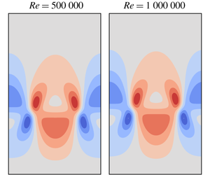
The invariant solution computed at $Re=1000$ is used as starting point for a continuation in Reynolds number where the size of the domain is kept constant in inner units, and therefore shrinks in outer units, when $Re$ is increased. As shown in figure 2, we can continue the solution up to $Re=1\,000\,000$ with both size of the box and magnitude of the solution decreasing in outer units. Figure 3 shows contours of the streamwise-averaged wall-normal velocity of the invariant solution in inner units at different Reynolds numbers. The solution structures remain almost unchanged over a wide range of Reynolds number when expressed in inner units.

To provide context for the achieved value of $Re$, we characterise the scale separation of fully developed turbulent flow at the same imposed value of $Re$ and in a large domain. While ASBL has the advantage that the self-similar near-wall inner scale $\unicode[STIX]{x1D6FF}_{\unicode[STIX]{x1D70F}}$ is directly controlled by $Re$, determining the outer scale, commonly associated with the turbulent boundary layer thickness $\unicode[STIX]{x1D6FF}_{99}$, requires extensive turbulent simulations. To be domain independent, these simulations need to be carried out in domains considerably larger than the MFU to allow for structures in the outer region, including those large compared to the wavelength imposed by the periodic MFU box, to develop. Those simulations can only be carried out for moderate $Re$. Using large eddy simulations, Schlatter & Örlü (Reference Schlatter and Örlü2011) and Bobke et al. (Reference Bobke, Örlü and Schlatter2016) determined the turbulent boundary layer thickness of ASBL as $\unicode[STIX]{x1D6FF}_{99}=101$ for $Re=333$ and $\unicode[STIX]{x1D6FF}_{99}=290$ for $Re=400$. Khapko et al. (Reference Khapko, Schlatter, Duguet and Henningson2016) observed $\unicode[STIX]{x1D6FF}_{99}$ to grow linearly in $Re$ for values between 260 and 333. For higher $Re$, the evolution of the turbulent boundary layer thickness is unknown. Since $\unicode[STIX]{x1D6FF}_{\unicode[STIX]{x1D70F}}=0.001$ at the highest achieved Reynolds number, the fully developed turbulent flow at $Re=10^{6}$ has a scale separation of at least $290\,000$, even if the growth of the turbulent boundary layer thickness does not extend much beyond $Re\sim 400$.

Figure 2. Continuation of the invariant solution to high Reynolds numbers in outer units. Cross-flow kinetic energy per area of the wall $e_{cf}=1/(L_{x}L_{z})\int _{MFU}(v^{2}+w^{2})\,\text{d}x\,\text{d}y\,\text{d}z$ in the MFU as a function of $Re$. Note that, in outer units, velocities are non-dimensionalised by $U_{\infty }$ and lengths by $\unicode[STIX]{x1D708}/V_{s}$, so $e_{cf}$ is in units of $U_{\infty }^{2}\unicode[STIX]{x1D708}/V_{s}$. The red dot indicates where the solution has been identified by edge tracking (see also inset for a magnification of the relevant parameter range). Visualisations of the invariant solution show contours of the streamwise-averaged wall-normal velocity at $Re=10\,000$, $40\,000$, $100\,000$, $200\,000$, $500\,000$ and $1\,000\,000$.

Figure 3. Invariant solution visualised in inner units. Contours of streamwise-averaged wall-normal velocity, normalised by friction velocity $u_{\unicode[STIX]{x1D70F}}$ at the same values of $Re$ as in figure 2. The contour levels are $v^{+}=v/u_{\unicode[STIX]{x1D70F}}=\{\pm 0.015,\pm 0.045,\pm 0.075,\pm 0.105,\pm 0.135\}$. The solution is localised at the wall so that only the lower half of the numerical domain is shown.

Figure 4. Three-dimensional structure of the invariant near-wall solution at $Re=40\,000$. The travelling wave is dominated by a strong low-speed streak (situated in the centre of the figure) sandwiched between weaker high-speed streaks located closer to the wall and flanked by alternating mirror-symmetric pairs of counter-rotating vortices. The low-speed streak is visualised by the green streamwise velocity isosurface ($u=0.2\,U_{\infty }$). Vortices are indicated by streamwise vorticity isosurfaces of $\unicode[STIX]{x1D714}_{x}$ at half of the maximum value with red/blue for positive/negative values. Due to the localisation of the structures near the wall, only the lower half of the computational domain is shown.

Figure 5. Amplitude of the first three streamwise Fourier modes of the invariant solution expressed in inner units ($\Vert \boldsymbol{u}_{0}^{+}(\,y,z)\Vert _{2}$, $\Vert \boldsymbol{u}_{1}^{+}(\,y,z)\Vert _{2}$ and $\Vert \boldsymbol{u}_{2}^{+}(\,y,z)\Vert _{2}$) as a function of $Re$. The amplitudes approach constant values indicating a solution that scales in inner units. The zero Fourier mode ($m=0$) dominates indicating a predominantly downstream invariant solution.

At high $Re$ the converged invariant solution remains localised near the wall. The structure of the travelling wave solution is dominated by spanwise-periodic alternating low- and high-speed streaks flanked by counter-rotating vortical structures, as shown in figure 4 where we present the solution at $Re=40\,000$. The solution is dominated by streamwise oriented streaks. In figure 5 we quantify the streamwise variation of the flow field by the amplitudes of the first three streamwise Fourier modes ($\Vert \boldsymbol{u}_{0}^{+}(\,y,z)\Vert _{2}$, $\Vert \boldsymbol{u}_{1}^{+}(\,y,z)\Vert _{2}$ and $\Vert \boldsymbol{u}_{2}^{+}(\,y,z)\Vert _{2}$). For increasing $Re$ the inner-unit amplitudes approach constant values indicating a solution scaling in inner units. Moreover, the amplitude of the downstream independent zero mode is more than two orders of magnitude larger than the amplitude of the first mode and three orders of magnitude larger than the amplitude of the second mode. This confirms that the invariant solution is dominated by streamwise invariant structures.

The relatively small bending of the low-speed streak (see figures 4 and 5) of the identified near-wall invariant solutions is consistent with features of lower-branch solutions found at large scales in large domains with size typical of transitional (e.g. Wang, Gibson & Waleffe Reference Wang, Gibson and Waleffe2007) and turbulent large-scale motions (e.g. Rawat, Cossu & Rincon Reference Rawat, Cossu and Rincon2016). In boxes remaining constant in outer units, this type of Navier–Stokes solution assumes a critical-layer structure for high Reynolds numbers (Wang et al. Reference Wang, Gibson and Waleffe2007; Deguchi & Hall Reference Deguchi and Hall2014a,Reference Deguchi and Hallb; Park & Graham Reference Park and Graham2015) where the streaks’ unstable mode concentrates near the critical layer. In the present case, however, the entire solution is downscaled in height, lateral wavelength and global amplitude when the Reynolds number increases (figure 2). There is no modification of the internal structure or a concentration near the critical layer. The zeroth streamwise Fourier mode of the wall-normal velocity $v_{0}^{+}(\,y,z)$ (associated with the streamwise vortices inducing the streaks), as well as the first streamwise Fourier mode $v_{1}^{+}(\,y,z)$ (associated with the streaks’ instability mode) are asymptotically constant when expressed in inner units as $Re$ increases, as shown in figure 6.

Figure 6. Contours of the streamwise Fourier modes of the invariant solutions’ wall-normal velocity (coloured contour lines). The zeroth mode $v_{0}^{+}(\,y^{+},z^{+})$ panels (a,b) and the first mode $v_{1}^{+}(\,y^{+},z^{+})$ panels (c,d) shown in inner units at $Re=40\,000$ panels (a,c) and $Re=100\,000$ panels (b,d). The critical layer where the zeroth streamwise mode of the streamwise velocity equals the travelling wave’s phase speed ($u_{0}(\,y,z)=c$) is also shown (bold solid black line) as well as the levels $u_{0}(\,y,z)/c=0.6,1.4,1.8$ (dashed black lines). Only the lower half of the numerical box is shown.

The root-mean-squared (r.m.s.) velocity profiles of the travelling wave solution expressed in inner units asymptotically collapse onto a single curve when $Re$ is increased (figure 7). This provides further confirmation that the travelling wave solution scales in inner units.

Figure 7. Root-mean-squared (r.m.s.) profiles of the travelling wave solutions expressed in inner units $u_{i,rms}^{+}(\,y^{+})=[1/(L_{x}^{+}L_{z}^{+})\int _{0}^{L_{x}^{+}}\int _{0}^{L_{z}^{+}}(u_{i}^{+}(x^{+},y^{+},z^{+})-u_{i,mean}^{+}(\,y^{+}))^{2}\,\text{d}x^{+}\text{d}z^{+}]^{1/2}$ at Reynolds numbers equal to $10\,000$, $40\,000$, $100\,000$, $200\,000$, $500\,000$ and $1\,000\,000$. (a) The r.m.s. profiles of the streamwise velocity $u_{rms}^{+}$, (b) r.m.s. profiles of the wall-normal velocity $v_{rms}^{+}$, (c) r.m.s. profiles of the spanwise velocity $w_{rms}^{+}$. For increasing $Re$, the r.m.s. profiles asymptotically collapse, indicating scaling in inner units. Note that the variation of $Re$ over two orders of magnitude corresponds to a full order of magnitude change in the height and lateral wavelengths of the solution in outer units (cf. figure 2).

The small change of the solution with $Re$ (figures 3 and 6), the asymptotically constant values of inner-unit amplitudes (figure 5), and the asymptotically converging r.m.s. profiles (figure 7) provide strong evidence that the fully resolved travelling wave solution asymptotes towards a self-similar solution at high $Re$. To investigate if the solution indeed becomes independent of Reynolds number for $Re\rightarrow \infty$ when expressed in similarity variables defined by rescaled length and velocity scales, we use the friction velocity, $u_{\unicode[STIX]{x1D70F}}=U_{\infty }/\sqrt{Re}$, and the viscous unit, $\unicode[STIX]{x1D6FF}_{\unicode[STIX]{x1D70F}}=\unicode[STIX]{x1D6FF}^{\ast }/\sqrt{Re}$, to non-dimensionalise the evolution equations. The Navier–Stokes equation for the inner-unit velocity deviation from the laminar solution reads

(4.1)$$\begin{eqnarray}\frac{\unicode[STIX]{x2202}\boldsymbol{u}^{+}}{\unicode[STIX]{x2202}t^{+}}+\boldsymbol{U}^{+}\boldsymbol{\cdot }\unicode[STIX]{x1D735}\boldsymbol{u}^{+}+\boldsymbol{u}^{+}\boldsymbol{\cdot }\unicode[STIX]{x1D735}\boldsymbol{U}^{+}+\boldsymbol{u}^{+}\boldsymbol{\cdot }\unicode[STIX]{x1D735}\boldsymbol{u}^{+}=-\unicode[STIX]{x1D735}p^{+}+\unicode[STIX]{x1D6FB}^{2}\boldsymbol{u}^{+},\end{eqnarray}$$

where $\boldsymbol{u}^{+}$ is the non-dimensionalised velocity deviation vector, and $\boldsymbol{U}^{+}$ is the non-dimensionalised laminar solution. The non-dimensionalised laminar solution in ASBL

(4.2)$$\begin{eqnarray}\boldsymbol{U}^{+}=Re^{1/2}(1-\exp (-y^{+}Re^{-1/2}))\hat{\boldsymbol{e}}_{\boldsymbol{ x}}-Re^{-1/2}\hat{\boldsymbol{e}}_{\boldsymbol{ y}}\end{eqnarray}$$

is a function of the Reynolds number, $Re=U_{\infty }/V_{s}$, and the wall-normal coordinate, $y^{+}$. The boundary conditions for the velocity deviation from the laminar base flow are periodic in the streamwise and in the spanwise directions, and zero-velocity at both the lower and upper walls. In the rescaled system with the given governing equation and the boundary conditions expressed in inner units, only the laminar base flow depends on $Re$. For $Re$ tending to infinity, the laminar base flow within the numerical box asymptotes to $\boldsymbol{U}^{+}=y^{+}\hat{\boldsymbol{e}}_{\boldsymbol{x}}$ and thus no longer depends on the Reynolds number. Therefore, when $Re$ is large, the rescaled system in inner units loses any dependence on the Reynolds number, and any solution of the system approaches a self-similar solution. Thus, any invariant solution that can be continued to asymptotically high Reynolds numbers in a box which has a fixed size in inner units becomes asymptotically self-similar. This suggests that the invariant solution that we present in this paper represents a self-similar solution of the Navier–Stokes equations in the near-wall inner region of the asymptotic suction boundary layer flow at high Reynolds numbers.

The analysis shows that as $Re$ tends to infinity, the equations for ASBL solutions expressed in inner units lose the dependence on Reynolds number so that any solution of those equations is self-similar and scales in inner units. Remarkably, we also observe that the partial differential equations including boundary conditions that any wall-attached solution of ASBL satisfies at asymptotically high $Re$, are identical to those describing plane Couette flow (PCF) at a value of the typically used Couette Reynolds number $Re_{PCF}={H^{+}}^{2}/4$, based on half the gap height and half the velocity difference. Boundary conditions of ASBL enforce zero wall-parallel velocity and a non-zero wall-normal suction. Expressed in inner units the suction velocity is $V_{s}^{+}=1/\sqrt{Re}$. For large $Re$, suction effects thus vanish and, asymptotically, the standard no-slip boundary conditions of PCF are reached. Consequently, at asymptotically high $Re$, any wall-attached solution of ASBL corresponds to a wall-attached solution of PCF. The value of the Couette control parameter $Re_{PCF}$ formally depends on the arbitrarily chosen $H^{+}$ reflecting the fact that a solution localised at the wall only depends on the shear rate at the wall while the distance of the second upper wall and thereby the value of $Re_{PCF}$ is irrelevant. Thus, at asymptotically high $Re$, all state-space structures representing wall-attached flow fields in the MFU of ASBL have counterparts in high Reynolds number PCF, such as those identified by Eckhardt & Zammert (Reference Eckhardt and Zammert2018). This suggests that the relevant state-space structures for near-wall turbulence that we identified in ASBL are universal in that they are not only independent of $Re$ when expressed in inner units but also do not depend on the specific shear-flow system considered. In fact, at sufficiently high $Re$, close to the wall, any wall-bounded shear flow is characterised by a universal shear profile, indistinguishable from PCF or ASBL and thus supports the same wall-attached solutions. This suggests that the entire state space of the near-wall region including the invariant solutions and their dynamical connections become independent of $Re$ and independent of the flow system. If invariant solutions, their heteroclinic connections and the entire state-space structures are universal, the deterministic dynamics supported by those structures is also universal. This provides an explanation of the well-known fact that at sufficiently high flow speeds the statistics of near-wall turbulence becomes independent of the flow system.

5 Conclusion and discussion

The aim of this work is to demonstrate the existence of an exact invariant solutions of the Navier–Stokes equations that capture spatial scales typical of turbulent motions in the near-wall region of a boundary layer at high Reynolds numbers. In a minimal flow unit of ASBL, chosen to capture the energetic scales of near-wall turbulent motions, a wall-attached travelling wave solution has been computed by edge tracking at $Re=1000$. We exploit the fact that ASBL allows us to express the viscous length scale $\unicode[STIX]{x1D6FF}_{\unicode[STIX]{x1D70F}}$ of the developed turbulent state in terms of the Reynolds number. We thus continued the solution to high $Re$ in the minimal flow unit, whose size remains constant in inner units but shrinks in outer units for increasing $Re$. The fully resolved solution can be followed up to $Re=1\,000\,000$. We provide numerical and theoretical evidence that the invariant solutions become exactly self-similar as $Re$ tends to infinity. Remarkably, the solution scales in inner units so that the individual fully resolved invariant solution of the Navier–Stokes equations captures the self-similar behaviour characteristic of near-wall-turbulent statistics. Moreover, in the high-$Re$ asymptotic limit, solutions of ASBL simultaneously constitute solutions of plane Couette flow thus reflecting the universality of near-wall turbulence.

Assuming that all relevant invariant solutions capturing near-wall motions can be continued to asymptotically high $Re$, our analysis suggests that entire state-space structures, including invariant solutions and their dynamical connections, become independent of Reynolds number when expressed in inner units. To provide further support for this picture, future research should aim at computing increasingly more complex state-space structures underlying near-wall turbulence in the high-$Re$ limit captured by the evolution equations expressed in inner units. This includes periodic orbits as well as orbits connecting invariant solutions.

Since the governing equations rescaled in inner units become asymptotically independent of Reynolds number, the complexity of the state space of near-wall turbulence and the number of relevant invariant solutions may not increase with $Re$ but remain constant, leading to a saturation of complexity in the near-wall region of turbulent flows. Such a saturation of complexity cannot be expected in the outer region of turbulent flows. It may thus be possible to eventually provide a predictive and quantitative description of turbulence in terms of a manageable number of invariant solutions (Chandler & Kerswell Reference Chandler and Kerswell2013; Cvitanović et al. Reference Cvitanović, Artuso, Mainieri, Tanner and Vattay2016) not only for transitional flows but also for the universal near-wall region of wall-bounded turbulence at very high Reynolds numbers. The self-similar exact invariant solution in the near-wall region of a boundary layer reported here is a significant step towards extending the invariant solution approach to turbulence from transitional flows to near-wall region of fully developed boundary layers.