NOMENCLATURE
- b
span of wing
- c(y)
chord distribution, spanwise
-
 $\bar{c}$
 mean aerodynamic chord
- C
nondimensional aerodynamic derivatives of flight dynamic states and structural modes
-
$\vec{d}$
elastic deformation of wing
- e
distance between elastic axis and aerodynamic center
- E
young's modulus
- I
moment of inertia
- m
weight of the drone
- mc(x)
mass distribution, chordwise
- mi
generalised mass of the ith structural mode
- p
rolling rate
- q
pitching rate
- Q
dynamic pressure
- Q ηi
generalised aerodynamic force of the ith structural mode
- S
reference area
- th(x)
membrane thickness distribution along sidewise
- u0
cruising speed
- α
angle of attack
- ηi
generalised coordinate of the ith structural mode
-
${\vec{\phi }_i}$
the ith structural mode shape
- ζi
the ith structural mode damping
- ωi
the ith structural mode frequency


1.0 INTRODUCTION
The requirements for Small Unmanned Aerial Vehicle (SUAV) have increased in many application areas, such as aerial photography and filming(Reference Beard and McLain1-Reference Chabot and Bird3). However, these vehicles lack the ability to endure significant atmospheric disturbance and usually have drastic dynamic responses in response to gusts, affecting the stability of the attitude and the flight path of the SUAV. This sensitivity to conditions is due to their small size and low Reynolds number flight, and restricts the development and application of these aerial vehicles. The low Reynolds number indicates a relatively low airspeed, which may be the same order of magnitude as the gust speed. Because of this, a gust can create a large change of Angle-of-Attack (AoA for short), leading to greater aerodynamic perturbance. The low Reynolds number also indicates the small size, weight and even a lower moment of inertia in every direction, making the overload and attitude response more sensitive to any perturbance.
Large- or medium-sized birds share similar Reynolds numbers with small-sized UAVs during flight. However, these birds seem to have a better ability to maintain their flight stability against gusts, even with a much smaller tail(Reference Videler4). Besides the extremely complex active control system of these natural creatures, which can hardly be imitated by the artificial system, the elasticity of their wings may also contribute to this stability. There have been previous studies of the aeroelastic properties of bird wings. Carruthers et al. studied the landing process of a golden eagle(Reference Carruthers, Thomas and Taylor5). They found that a small part of the feather beneath the leading edge of the eagle's wing can deform with the change of aerodynamic conditions and the flight regime. The deformation of the feather can be considered aeroelastic deformation that can provide additional lift and delay flow separation during the landing process.
A membrane wing is a type of wing with thin aerofoils, like a bird wing. This type of wing is widely used in the designs of small and micro aerial vehicles because low weight is required to maximise the carried load. One typical example is the Maveric unmanned aircraft system developed by Prioria Robotics(6). It is a portable SUAV that can be widely used for multiple types of missions. Another example is the GenMAV developed by the US Air Force Research Laboratory and the University of Florida. It is able to fly through an urban area agilely to provide reconnaissance(Reference Cantrell, LaCroix and Ifju7-Reference Arce9).
Similar to avian flight, aeroelastic effects may exist in the flight of membrane-wing-containing SUAVs because of the limited stiffness of the wing. The natural frequency of flight dynamic modes may be relatively high due to the small value of the moment of inertia, and the natural frequency of aeroelastic modes are low because of the flexibility of the membrane wing. The gap of the natural frequency can become small and there may be considerable coupling between the two types of modes through both static and dynamic aeroelastic effects. Lind et al. investigated the flight dynamic of the GenMAV with aeroelastic coupling using the numerical tool ASWING(Reference Drela10). These studies concluded that the elasticity of the wing is detrimental to the longitudinal stability of the flight dynamic(Reference Babcock and Lind11), and can also be harmful to the control law design(Reference Tseng12). Hesse et al. reached a similar conclusion about the coupling dynamic(Reference Hesse and Palacios13). These studies show that the original idea to utilise the elasticity of the wing to alleviate gust perturbance and improve flight stability has not yet been fully accomplished, although the membrane wing has the geometric shape of a bird's wing.
This study aimed to optimise the flight dynamic properties by focusing on aeroelastic effects of a bio-inspired membrane wing. In addition to the geometric imitation, the bird wing's structural dynamic properties are included in the optimisation of the wing. An analytical modelling method was applied to analyse the coupling between the aeroelastic modes and the flight dynamic modes. Unlike numerical tools like ASWING, utilised in the GenMAV relevant research, here an analytical modelling method with more transparency was used. This provides the possibility to investigate how the specific features of the bio-inspired wing affect the coupling between aeroelasticity and flight dynamics. A similar method was recently used in the famous X-56A project for the coupling of flight dynamic modelling and analysis(Reference Schmidt14,Reference Schmidt15) . Although there are some assumptions, the accuracy of this modelling method was demonstrated by the accurate prediction of the body-freedom flutter speed of an X-56A precursor.
There are six sections in this paper. The second section describes the general properties of the prototype. Section 3 depicts the coupling dynamic of the prototype. In this section, the bio-inspired properties are summarised and their influences on the structural dynamic of the wing are described. In Section 4, different structural properties are addressed to discuss how the bio-inspired wing features affect the flight dynamics, especially when the inertial and elastic axis position change in the chordwise direction. Section 5 shows the gust response results and demonstrates the effectiveness of the bio-inspired wing. Section 6 presents the conclusions.
2.0 GENERALISED DESCRIPTION OF THE PROTOTYPE
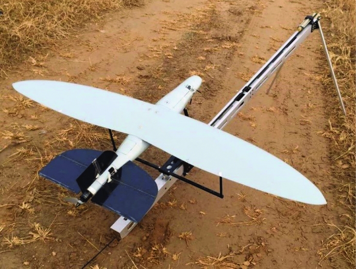
The prototype of this research is shown in Fig. 1, and its general parameters are listed in Table 1. The bio-inspired membrane wing of the prototype, which is the most important feature, is discussed in the following sections in detail. In addition to the wing, this aerial vehicle is characterised by its biomimetic general aerodynamic configuration, including the small tails, the short distance between CG and the tails, and the fusiform fuselage. The fuselage length and tail areas are relatively small, and the distance between the tails and the center of gravity is short, making the vehicle suitable as a portable canister launcher. There is a fusiform fuselage with a bigger diameter in the middle and two pointy ends. This design is a compromise between drag reduction and the miniaturisation of these components in the fuselage. All these features make the aerodynamic configuration more similar to a large-size gliding bird rather than an artificial fixed-wing aircraft. However, it is difficult in this design to guarantee static stability by rearranging the CG position. Thus, it is also important to augment the flight dynamic stability through the dynamic deformation of the elastic wing when traditional methods of stabilisation cannot be used.

Figure 1. The bio-inspired wing SUAV prototype.
Table 1 General parameters of the prototype

3.0 FLIGHT DYNAMIC MODELLING OF THE BIO-INSPIRED WING PROTOTYPE INCLUDING AEROELASTIC COUPLING
An analytical, linear-time-invariant (LTI for short) model was built to investigate the coupling between the aeroelasticity of the bio-inspired wing and flight dynamics. The modelling process includes three parts: rigid-body flight dynamic modelling, wing structural dynamic modelling, and the modelling of coupling properties. The rigid-body flight dynamic was modelled by the classic method and formulated as a form of state-space(Reference Zhang16).
3.1 Structural dynamics of the bio-inspired wing
Figure 2 shows the two types of membrane wings designed for the prototype. Image (a) shows the original membrane wing with an average membrane thickness, and image (b) shows the optimised wing with stiff ribs in the chordwise orientation and the forward positions of the inertial axis and elastic axis. The thin aerofoil, the ribs and the forward axis positions are all inspired by a bird's wing. Appendix A presents the geometric and material information in detail.
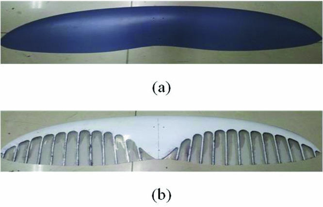
Figure 2. Two types of membrane wings for the prototype.
First, the finite element model (FEM for short) of the first wing design (shown in Fig. 2(a)) was established for structural dynamic modelling. Model analysis based on the FEM can deconstruct the dynamic deformation of all these elements in FE model as the linear combination of several independent modes with different natural frequencies as follows:
 $$\begin{equation}
\vec{d}(x,y) = \sum\limits_i^\infty {{\eta _i}{{\vec{\phi }}_i}(x,y)}
\end{equation}$$
$$\begin{equation}
\vec{d}(x,y) = \sum\limits_i^\infty {{\eta _i}{{\vec{\phi }}_i}(x,y)}
\end{equation}$$
Where ηi represents the generalised mode coordinates. The subscript i represents the mode whose natural frequency is the ith lowest of all the modes. Only the first three modes are considered in this case and the ones with higher frequencies are ignored because they are rapidly attenuated by damping and will not be exhibited in most practical cases. Here, they are also ignored because their frequencies are too far from the flight dynamic frequencies so the coupling effect is negligible.  ${\vec{\phi }_i}(x,y)$ is the mode shape. The first few mode shapes represent the major characters of the structure's dynamic motion. After model analysis, these decoupled motions can be depicted as:
 $$\begin{equation}
\frac{{d{{\dot{\eta }}_i}}}{{dt}} + {\zeta _i}{\omega _i}{\dot{\eta }_i} + {\omega _i}^2{\eta _i} = \frac{{\sum_{j = 1}^n {{Q_{{\eta _j}}}} }}{{{m_i}}},
\end{equation}$$
$$\begin{equation}
\frac{{d{{\dot{\eta }}_i}}}{{dt}} + {\zeta _i}{\omega _i}{\dot{\eta }_i} + {\omega _i}^2{\eta _i} = \frac{{\sum_{j = 1}^n {{Q_{{\eta _j}}}} }}{{{m_i}}},
\end{equation}$$
where the ωi, ζi and mi are the frequency, the damping and the generalised mass of the mode, respectively. Q ηj is the generalised aerodynamic force for the jth mode. Equation (2) presents the aeroelastic properties of the wing.
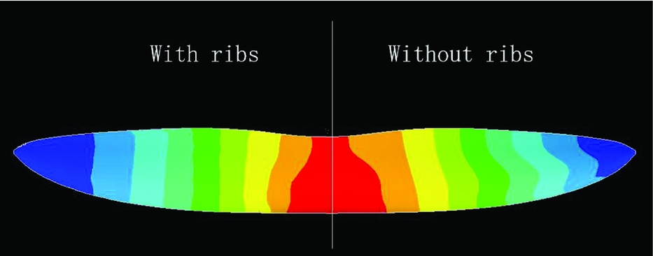
Figure 3 demonstrates the first mode shape of the wing  ${\vec{\phi }_i}$. For convenience of comparison, in this figure the mode shape of the wing with ribs is presented as the right half-wing and the corresponding wing without ribs is presented as the left half. It is necessary to note that the right half and left half of the wing are actually symmetric in all cases in this paper. When the mode shape shown in a figure differs from that on the other half-wing, it is only to easily compare the different symmetric mode shapes. The root chord is fixed because the inertial force coupling between the wing and the fuselage is neglected because the membrane wing is light in weight (less than 10% of the overall weight). Figure 3 shows that with or without ribs on the wing, the first mode of the wing is always a twist-dominated one.
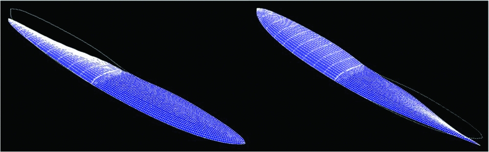
Figure 3. The first mode shape of the wing with and without ribs.
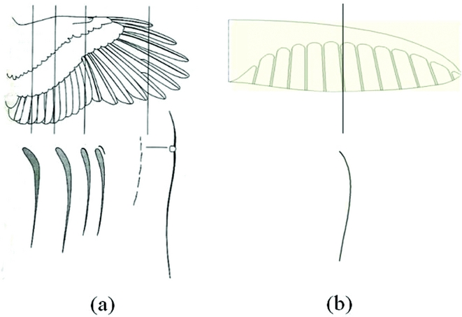
Generally, the first structural mode of a wing is always a bending dominated one due to its geometric features. However, as a bio-inspired thin aerofoil, here it is a twisting-dominated mode shape. This is because the aerofoil of the membrane wing is designed to be similar to the aerofoil of a bird's wing, as depicted in Fig. 4. When there is an external torque applied to the wing, the area surrounded by the torsional shear flow Fig. 5(b) can be much smaller compared with the regular-wing-box aerofoil for aerofoil planes (in Fig. 5(a)). Therefore, the thin aerofoil will greatly decrease the twisting stiffness. Vos. et al used a similar principle to adjust the twisting stiffness of the wing(Reference Vos, Gurdal and Abdalla17). This approach can greatly influence the aerodynamics of the aerial vehicle, because the twisting deformation angle can directly affect the local AoA on the wing, causing greater coupling between the aeroelasticity of the wing and the flight dynamics of the whole plane. The following sections will explain how these structural dynamic properties affect the coupling between them.

Figure 4. The thin aerofoil of bird's wing (a) and the membrane wing of the prototype (b).
Figure 5. The torsion shear flow on a wing box aerofoil (a) and thin aerofoil (b).
The different colors in Fig. 6 depict the relative twisting deformation amount in the first mode shape. In both cases, the twisting deformation changes smoothly along the spanwise orientation, with nearly no twisting deformation change in the chordwise direction at an arbitrary location in the spanwise direction. This means that basically, the aerofoil shape has no distortion. That is convenient for aerodynamic modelling and aeroelastic derivative calculations because the quasi-steady aerodynamic change induced by the deformation can be easily linearised.

Figure 6. Twist deformation of the first mode shape.
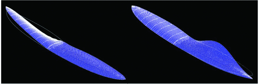
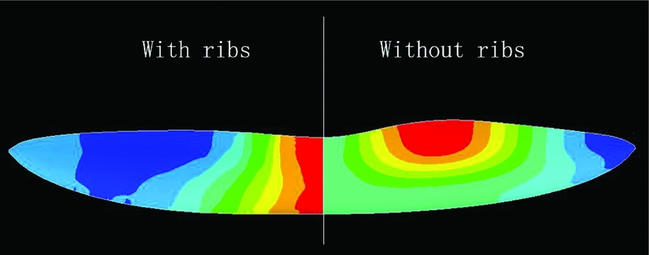
Similarly, Figs. 7 and 8 show the second mode shapes, in which twisting deformation remains the most significant component. However, the wing ribs can make a big difference in this case. Without ribs, the twisting deformation changes greatly along the chordwise direction at the middle range of the span. In other words, the aerofoil deforms significantly. That deformation leads to non-linear aerodynamic change, which is difficult to formulate and integrate into the analytical dynamic model. This phenomenon becomes more significant when the parts near the tailing edge are adjusted to be more flexible. The chordwise ribs significantly decrease this phenomenon. The corresponding situation of the third structural mode is similar.

Figure 7. The second mode shape of the wing with and without ribs.

Figure 8. Twist deformation of the second mode shape.
The arrangement of stiff chordwise ribs imitates the rachis-barb structure of the flight feathers on a bird's wing. Figure 9 depicts this comparison. The rachis is stiff and helps to retain the aerofoil shape on all wing sections, and the barb is flexible material. In this design, there is hardly any elastic force along the spanwise direction, allowing maintenance of the aerofoil shape with low twisting stiffness. This is illustrated with the structural mode shapes presented in Figs. 7 and 8.
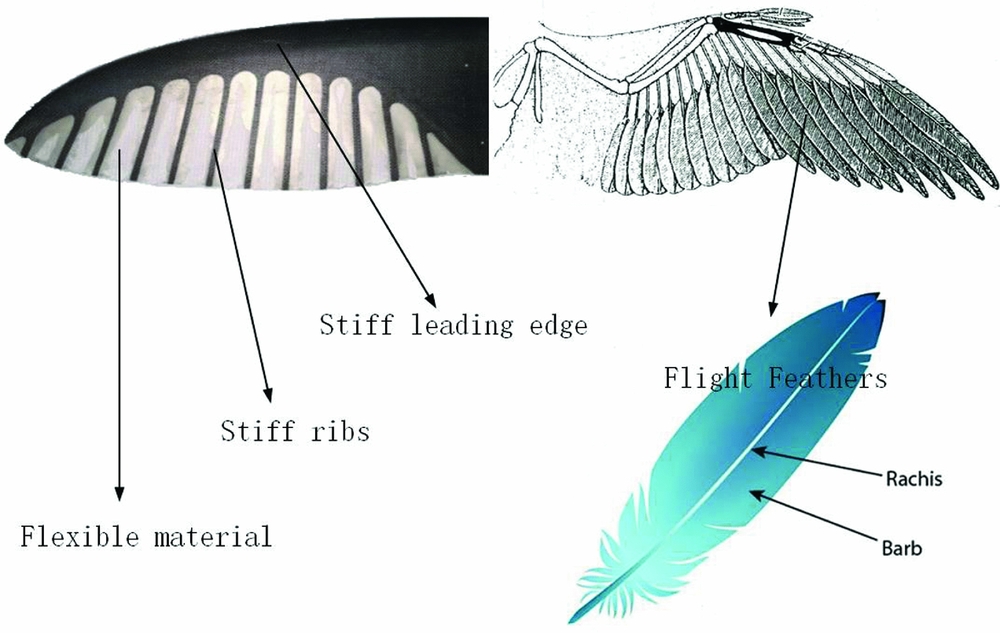
Figure 9. Flight feathers on a bird's wing and its structure.
The first three structural modes are considered here. Table 2 summarises their structural dynamic parameters and Figs. 10-12 present the corresponding mode shapes. Only the mode shapes for the wings with ribs are shown here and used in the following modelling work, as it is difficult to integrate some of the mode shapes without ribs into the LTI coupling model. The positive twisting direction is the leading edge upward and the positive bending direction is downward. Structural damping is neglected here since it is much lower than the aerodynamic damping.
Table 2 Structural dynamic parameters of the first three modes

Figure 10. The twisting and bending parts of the first mode shape.
Figure 11. The twisting and bending parts of the second mode shape.
Figure 12. The twisting and bending parts of the third mode shape.
3.2 The coupling flight dynamics of the prototype
Figure 13 presents the modelling framework of the coupling of rigid-body flight dynamics and structural dynamics. The contents in the dotted frame represent the classic flight dynamic modelling process. In practical cases, coupling can work through both structural dynamic forces and aerodynamic forces. Structural dynamic force coupling between two types of modes can be formulated by applying Lagrange equations on the overall coupling motions(Reference Schmidt14,Reference Haghighat, Martins and Liu18) . Here, the mean axes assumption is applied(Reference Meirovitch and Tuzcu19) and inertial coupling is neglected due to the small weight proportion of the membrane wing (less than 10%). The two kinds of modes are only coupled aerodynamically.

Figure 13. Schematic of the coupled dynamic modelling process.
In this study, the rigid-body flight dynamic motion is depicted using the traditional American reference system for aircrafts, and the motion of the elastic wing is modelled as a linear superposition of the rigid body motion on the root chord and the elastic wing motion, as it is described by Equation (3). The whole reference system is shown in Fig. 14. Since the stiffness ribs ensure no obvious aerofoil distortion in the first three mode shapes, the local AoA for one spanwise location can be depicted as a linear superposition of the states of both the flight dynamics (AoA, pitching rate, etc.) and the bending and twisting deformation of the structural dynamics (shown in Equation (3)) when the deformation amount is not significant enough to make it stall.
 $$\begin{equation}
{\alpha _{local}}(y) = \alpha + {\alpha _r} - q\left( {\frac{{{x_E} + e}}{{{u_0}}}} \right) + p\frac{y}{{{u_0}}} + \sum\limits_{i = 1}^3 {\left( {\frac{{d\phi _i^b}}{{dx}}{\eta _i} + \frac{1}{{{u_0}}}\phi _i^b{{\dot{\eta }}_i}} \right)} ,
\end{equation}$$
$$\begin{equation}
{\alpha _{local}}(y) = \alpha + {\alpha _r} - q\left( {\frac{{{x_E} + e}}{{{u_0}}}} \right) + p\frac{y}{{{u_0}}} + \sum\limits_{i = 1}^3 {\left( {\frac{{d\phi _i^b}}{{dx}}{\eta _i} + \frac{1}{{{u_0}}}\phi _i^b{{\dot{\eta }}_i}} \right)} ,
\end{equation}$$
p and q are the rolling and pitching speed of the aircraft, respectively. αr is the angle between the x-axis and root chord,  $\frac{{d\phi _i^b}}{{dx}}$ and ϕbi are the twisting and bending component of the ith mode shape, respectively. Fig. 14 shows the geometric meaning of other symbols.
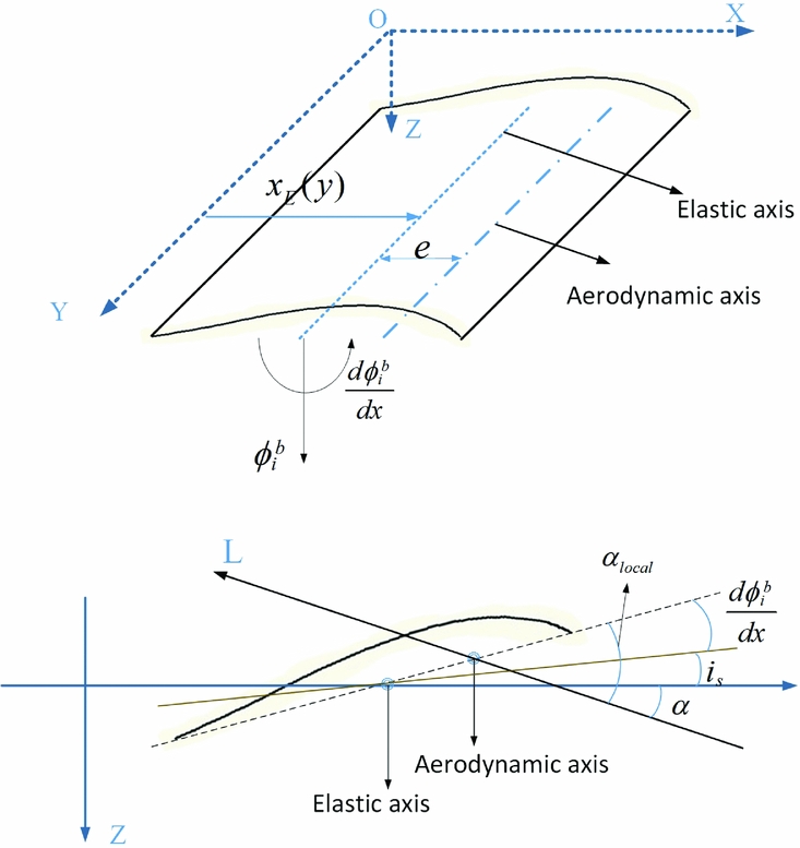
Figure 14. Geometric relationships between different parameters on the wing.
Classic vortex method theory(Reference Melin20) helps to estimate the aerodynamic distribution in the spanwise direction of the wing by integrating the mode shapes and aerodynamic distributions. The detailed definition process is the same as the one developed by Schmidt(Reference Schmidt21). However, there are some improvements, such as the derivations about  ${\dot{\eta }_i}$ are defined to maintain their non-dimensional properties so that their values will not change with changes in airspeed. Table A1 in Appendix A lists the vital aerodynamic derivatives of the structural mode coordinates.
After integrating the aerodynamics with structural dynamics together, the coupling flight dynamics can be depicted as the form of state-space:
 $$\begin{equation}
\dot{x} = Ax + G{w_g} = \left[ {\begin{array}{@{}*{3}{c}@{}} {{A_{RR}}}&{{A_{RE}}}&{{A_{R\dot{E}}}}\\ 0&0&I\\ {{A_{ER}}}&{{A_{EE}}}&{{A_{E\dot{E}}}} \end{array}} \right]\left[ {\begin{array}{@{}*{1}{c}@{}} {{x_R}}\\ {{x_E}}\\ {{{\dot{x}}_E}} \end{array}} \right] + \left[ {\begin{array}{@{}*{1}{c}@{}} {{G_R}}\\ 0\\ {{G_E}} \end{array}} \right]{w_g}
\end{equation}$$
$$\begin{equation}
\dot{x} = Ax + G{w_g} = \left[ {\begin{array}{@{}*{3}{c}@{}} {{A_{RR}}}&{{A_{RE}}}&{{A_{R\dot{E}}}}\\ 0&0&I\\ {{A_{ER}}}&{{A_{EE}}}&{{A_{E\dot{E}}}} \end{array}} \right]\left[ {\begin{array}{@{}*{1}{c}@{}} {{x_R}}\\ {{x_E}}\\ {{{\dot{x}}_E}} \end{array}} \right] + \left[ {\begin{array}{@{}*{1}{c}@{}} {{G_R}}\\ 0\\ {{G_E}} \end{array}} \right]{w_g}
\end{equation}$$
The rigid state vector xR = [u α q θ]T represents the longitudinal dynamic motions. u, α, q, θ are the flight speed, AoA, pitching rate and pitching angle, respectively. xE = [η1 η2 . . . ηn]T is the state vector of elastic deformation. wg is the vertical airspeed induced by gusts. The matrix ARR indicates the longitudinal flight dynamic properties, AEE and AEĖ indicate aeroelastic properties of the flexible wing, and ARE, ARĖ, AER indicate the coupling between them. The detailed submatrixes are shown in the Appendix B.
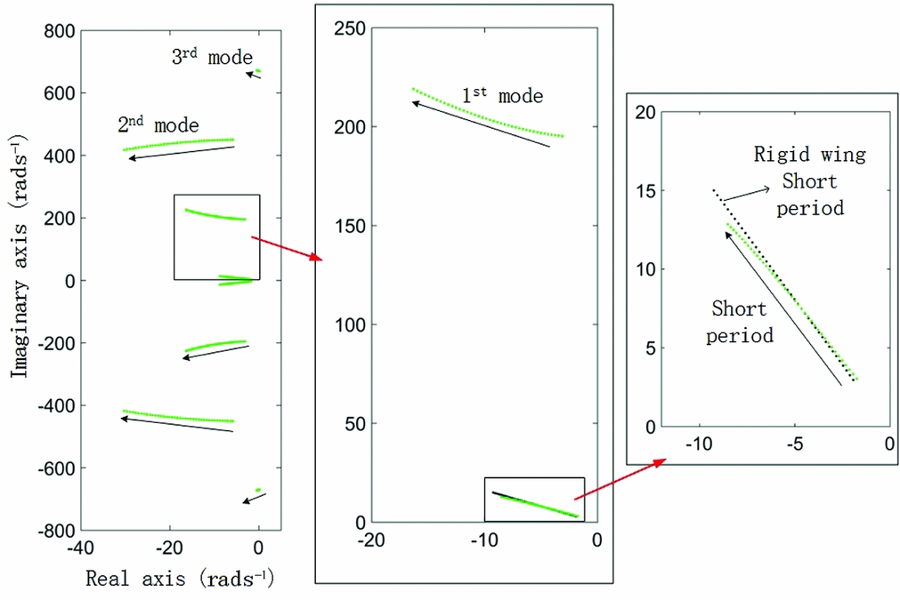
First, the original prototype of the wing in Fig. 2(a) was modelled for coupling dynamic analysis. The left image in Fig. 15 presents the eigenvalues of matrix A in Equation (4). The green data points present one pair of short-period dominated eigenvalues and three pairs of structural dominated eigenvalues when the airspeed changes from 5 ms−1 to 25 ms−1. The pair of phugoid-dominated eigenvalues is not presented here because the vortex lattice method cannot effectively approximate the drag distribution, which is vital for phugoid analysis. Additionally, the phugoid model has little coupling with other modes due to its very low natural frequency. The arrows show how these eigenvalues change with increasing airspeed. When the flight speed is increasing, the frequency of the 1st aeroelastic model increases and it can combine with the 2nd mode and lead to a regular flutter at a higher airspeed.

Figure 15. Eigenvalues of coupling dynamic systems at various flight speeds.
The central image of Fig. 15 shows that due to the growth of the 1st mode frequency, the short-period dominated mode becomes less sensitive and more stable. The black data points in the right image of Fig. 15 represent the corresponding eigenvalues (eigenvalues of the matrix ARR in Equation (4)) under the rigid-wing assumption. The difference between the green data points and the black ones shows that the effect of aeroelastic coupling can still be considerable even for a large frequency gap between short-period and aeroelastic modes. There are two primary factors which cause this kind of effects: the sign and value of the coefficient C Q 1η1, presented in Table A1 in the Appendix B.
If the coupling between the 1st aeroelastic mode and other modes is temporarily neglected (only for the coupling analysis), then Equation (2) can be rewritten as:
 $$\begin{equation}
\frac{{{d^2}{{\dot{\eta }}_1}}}{{d{t^2}}} + \left( {{\zeta _1}{\omega _1} - {H_{1{{\dot{\eta }}_1}}}} \right)\frac{{d{\eta _1}}}{{dt}} + \left( {{\omega _1}^2 - {H_{1{\eta _1}}}} \right){\eta _1} = 0
\end{equation}$$
$$\begin{equation}
\frac{{{d^2}{{\dot{\eta }}_1}}}{{d{t^2}}} + \left( {{\zeta _1}{\omega _1} - {H_{1{{\dot{\eta }}_1}}}} \right)\frac{{d{\eta _1}}}{{dt}} + \left( {{\omega _1}^2 - {H_{1{\eta _1}}}} \right){\eta _1} = 0
\end{equation}$$
After utilising the Laplace transform, and neglecting the structural dumping ζ, the eigenvalues can be solved as:
 $$\begin{equation}
\lambda = \frac{1}{2}{H_{1{{\dot{\eta }}_1}}} \pm \frac{1}{2}\sqrt {{H_{1{{\dot{\eta }}_1}}}^2 + 4{H_{1{\eta _1}}} - 4{\omega _1}^2}
\end{equation}$$
$$\begin{equation}
\lambda = \frac{1}{2}{H_{1{{\dot{\eta }}_1}}} \pm \frac{1}{2}\sqrt {{H_{1{{\dot{\eta }}_1}}}^2 + 4{H_{1{\eta _1}}} - 4{\omega _1}^2}
\end{equation}$$
According to the generalised aerodynamic parameter definitions in Tables A1 and A2:
 $$\begin{equation}
{H_{1{\eta _1}}} = \frac{{C_{{\eta _1}}^{{Q_1}}QSc}}{{{m_1}}} = \frac{{{\rho _a}u_0^2}}{{2{m_1}}}\int\limits_{{ - b/2}}^{{b/2}}{{\left( {\frac{{d\phi _1^b}}{{dx}}} \right)(e\frac{{d\phi _1^b}}{{dx}} - \phi _1^b){C_{l\alpha }}cdy}},
\end{equation}$$
$$\begin{equation}
{H_{1{\eta _1}}} = \frac{{C_{{\eta _1}}^{{Q_1}}QSc}}{{{m_1}}} = \frac{{{\rho _a}u_0^2}}{{2{m_1}}}\int\limits_{{ - b/2}}^{{b/2}}{{\left( {\frac{{d\phi _1^b}}{{dx}}} \right)(e\frac{{d\phi _1^b}}{{dx}} - \phi _1^b){C_{l\alpha }}cdy}},
\end{equation}$$
 $$\begin{equation}
{H_{1{{\dot{\eta }}_1}}} = \frac{{C_{{{\dot{\eta }}_1}}^{{Q_1}}QS{{\bar{c}}^2}}}{{2{m_1}{u_0}}} = \frac{{{\rho _a}{u_0}}}{{2{m_1}}}\int\limits_{{ - b/2}}^{{b/2}}{{\phi _1^b(e\frac{{d\phi _1^b}}{{dx}} - \phi _1^b){C_{l\alpha }}cdy}}
\end{equation}$$
$$\begin{equation}
{H_{1{{\dot{\eta }}_1}}} = \frac{{C_{{{\dot{\eta }}_1}}^{{Q_1}}QS{{\bar{c}}^2}}}{{2{m_1}{u_0}}} = \frac{{{\rho _a}{u_0}}}{{2{m_1}}}\int\limits_{{ - b/2}}^{{b/2}}{{\phi _1^b(e\frac{{d\phi _1^b}}{{dx}} - \phi _1^b){C_{l\alpha }}cdy}}
\end{equation}$$
In Equation (6), because the 1st mode shape is a twisting dominated one (which means  $\frac{{d\phi _1^b}}{{dx}}$ is dominant) and ω1 is relatively small, the sign of C Q 1η1 and H 1η1 determinate whether the mode frequency will increase or decrease when the airspeed increases, and their values determinate the speed of this frequency change. The sign and value of C Q 1η1 is determined by the chordwise position of the elastic axis and the inertial axis of the wing. The elastic axis position primarily affects the e and the inertial axis position primarily influence the proportion of
  $\frac{{d\phi _1^b}}{{dx}}$ and ϕb1 (shown in Fig. 13). For the original design, the twisting part and bending part of the 1st mode shape are counteracted by each other in calculation of the virtual work (shown in Figs. 3 and 9). So the value of C Q 1η1 is only −0.03, which means the frequency becomes higher with a relatively slow rate when the airspeed increases. Furthermore, this frequency increase can cause a corresponding decrease of the short period frequency in the coupling dynamics, as the product of all eigenvalues remains constant (the determinant of the matrix A) at a certain airspeed. Other modes have very high ωi values and their frequencies are hardly affected during low-speed flight.
A reduced order model with quasi-static deformation(Reference Schmidt14) was also applied to more precisely estimate the short-period properties, as the short-period-dominated modes shown in the right image of Fig. 15 have elastic deformation components and cannot precisely represent the longitudinal flight dynamics. Assuming that there is only quasi-static deformation (QSD for short) in the short-period oscillation process, the order of Equation (4) can be reduced as:
 $$\begin{equation}
{\dot{x}_R} = {A_{QSD}}{x_R} + {G_{QSD}}{w_g},
\end{equation}$$
$$\begin{equation}
{\dot{x}_R} = {A_{QSD}}{x_R} + {G_{QSD}}{w_g},
\end{equation}$$
where
 $$\begin{equation}
\begin{array}{@{}l@{}} {A_{QSD}} = {A_{RR}} - {A_{RE}}A_{EE}^{ - 1}{A_{ER}}\\ {G_{QSD}} = {G_R} - {A_{RE}}A_{EE}^{ - 1}{G_E} \end{array}
\end{equation}$$
$$\begin{equation}
\begin{array}{@{}l@{}} {A_{QSD}} = {A_{RR}} - {A_{RE}}A_{EE}^{ - 1}{A_{ER}}\\ {G_{QSD}} = {G_R} - {A_{RE}}A_{EE}^{ - 1}{G_E} \end{array}
\end{equation}$$
The red data points shown in Fig. 16 are the eigenvalues of the matrix AQSD when the air velocity varies from 5 ms−1 to 25 ms−1. The blue data points and green data points represent the eigenvalues of matrix ARR and A, respectively. The results from the coupling model and the QSD model are similar. Therefore, the conclusions from Fig. 15 have good validity. The aeroelasticity of the wing affects the short period mostly through quasi-static aeroelastic deformation when there is a considerable frequency gap between the two types of modes. More detailed mode characteristics at different airspeeds are presented in Table 3.
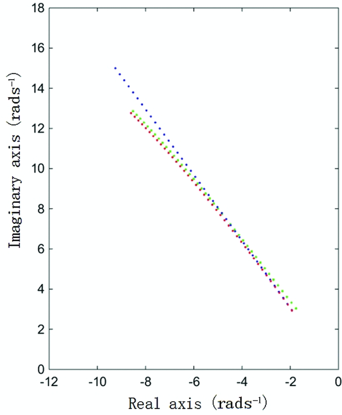
Figure 16. Short period eigenvalues of three different models.
Table 3 Mode properties under different analysis types and airspeeds

4.0 COUPLING ANALYSIS FOR INERTIAL AND ELASTIC FEATURES OF THE WING
4.1 Coupling flight dynamic analysis with backward axis positions
Another feature of a bird wing is the forward location of the inertial axis and elastic axis, which can be estimated by Equations (11) and (12). The xleading and xtailing represent the leading end and the trailing end position of the aerofoil plane, respectively. The xI and xE are the position of the inertial axis and elastic axis, respectively. mc(x) is the mass in a unit area. th(x) is the thickness of the aerofoil. Δθt is an assumed small twisting deformation on this aerofoil plane due to an external pure torque. Figure 17 shows the geometric relationship between those items. E is the Young's modulus of the structure,
 $$\begin{equation}
\int_{{{x_{{\rm{trailing}}}}}}^{{{x_{{\rm{leading}}}}}}{{(x - {x_I}){m_c}(x)th(x)dx}} = 0,
\end{equation}$$
$$\begin{equation}
\int_{{{x_{{\rm{trailing}}}}}}^{{{x_{{\rm{leading}}}}}}{{(x - {x_I}){m_c}(x)th(x)dx}} = 0,
\end{equation}$$
 $$\begin{equation}
\int_{{{x_{{\rm{trailing}}}}}}^{{{x_{{\rm{leading}}}}}}{{(x - {x_E})E(x)th(x)\Delta {\theta _t}dx}} = 0
\end{equation}$$
$$\begin{equation}
\int_{{{x_{{\rm{trailing}}}}}}^{{{x_{{\rm{leading}}}}}}{{(x - {x_E})E(x)th(x)\Delta {\theta _t}dx}} = 0
\end{equation}$$
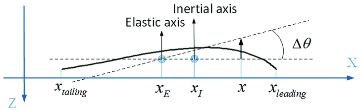
Figure 17. The chordwise position of the inertial and elastic axes.
Figures 4(a) and 9 show that the parts near the leading edge of the bird's wing are thicker and are made of bones and muscles with high stiffness and weight. The parts behind are extended by flight feathers that are very light and do not provide any stress in the spanwise direction. Therefore, the values of E(x), t(x), and m(x) are higher near the leading edge and it is reasonable that xI and xE are located near the leading edge. The membrane wing shown in Fig. 2(b) exhibits these properties.
Based on the FEM of the wing shown in Fig. 2(a) with homogenous membrane thickness, the inertial and elastic axis positions of the wing are adjusted for the parameter sensitivity analysis. Fig. 18 shows the eigenvalues of the coupling dynamic system when the two axes are separately adjusted backward. The corresponding parameters C Q 1η1 are adjusted to 0.1 in both cases.
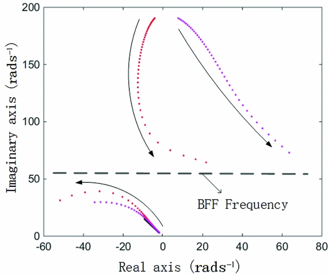
Figure 18. Eigenvalues of the coupling flight dynamic with backward axes position.
In Fig. 18, the red data points show the corresponding eigenvalues when the inertial axis is moved backward (about 0.3~0.35 of the chord from original location). In this case, the first aeroelastic mode frequency decreases when the airspeed increases, opposite to the case shown in Fig. 14. This is because the sign of C Q 1η1 changes from negative to positive. Furthermore, due to the twisting domination in the first aeroelastic mode, the mode frequency drops rapidly, increasing the frequency of the short-dominated mode. The damping of the short-period dominated mode becomes smaller and the frequency becomes larger, meaning that the prototype becomes more unstable and more sensitive to gust perturbance.
As the decreasing rate of the 1st aeroelastic mode frequency and the increasing rate of the short-period frequency are fast, the frequency gap diminishes rapidly and then vanishes, and these two modes become strongly coupled as the airspeed reaches 20 ms−1. One of the modes then goes quickly across the imaginary axis at the airspeed of 23 ms−1. That phenomenon, body-freedom flutter (BFF)(Reference Richards22,Reference Leitner23) , usually appears when there is a fly-wing aerodynamic configuration, or a high aspect ratio wing with a large weight. This case proves that this special flutter condition can also occur for a small aircraft with a conventional aerodynamic configuration and a light wing because the natural frequency of the 1st structural mode with twisting dominated mode shape can decrease very fast due to the aerodynamic changes.
In Fig. 18, the purple data points show the corresponding case when the elastic axis is adjusted. The coupling properties are similar with those in the inertial adjusting case, except that these aeroelastic modes can very easily become unstable when the elastic axis is moved backward because the sign of  ${H_{1{{\dot{\eta }}_1}}}$ is changed.
The detailed short-period dominated mode properties for both cases under different conditions of airspeed are presented in Tables 4 and 5. These tables show that the eigenvalues obtained under QSD assumption are considerably different from the eigenvalues of the coupling model, since there is no longer a frequency gap and the two modes are strongly coupled through both the static and the dynamic aeroelastic deformation.
Table 4 Mode properties when the inertial axis is moved backward

Table 5 Mode properties when the elastic axis is moved backward

Table 6 Mode properties when the inertial axis is moved forward

Table 7 Mode properties when the elastic axis is moved forward
4.2 Coupled flight dynamic analysis with forward axis positions
Similar to the results in Fig. 8, the data in Fig. 19 shows the effect of moving the inertial axis (dark blue data points) and elastic axis (light blue ones) forward so that the parameter C Q 1η1 is adjusted to −0.1. Compared with the case presented in Fig. 18, where C Q 1η1 equals −0.03, the coupling effect is similar but stronger. For the short period, the damping becomes larger and the frequency becomes lower after the optimised adjustment in the structure, so it will more effectively alleviate gust response.
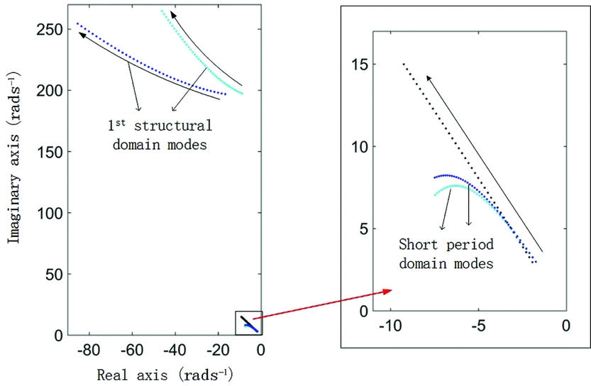
Figure 19. Eigenvalues of the coupled flight dynamics with axes position shifted backwards.
These results indicate that the conclusions made in Refs Reference Hesse and Palacios13 and Reference Schmidt14 are conditional. Whether the elasticity of wing has a beneficial or a detrimental effect on the short-period stability depends on the sign of C Q 1η1, which is greatly influenced by the chordwise inertial/elastic axis position of the wing. This shows that a wing with forward elastic and inertial axis positions, the features of a bird's wing, can effectively increase the longitudinal stability, and this effect will be amplified by the twisting dominated structural mode of the thin aerofoil wing.
5.0 GUST RESPONSE SIMULATION
The results in Section 4 can guide the structural optimisation of the wing. Figure 20 depicts the optimisation procedure. Figure 2(a) presents the original design of a wing with average membrane thickness. The new structure design with forward positions of the inertial axis and the elastic axis should improve flight dynamic characteristics and gust response. The FE model and VLM-based aerodynamic model introduced in Section 3 can predict static elastic deformation on the wing under wing loading. If the results indicate that there are structural failures or a stall at some points on the wing due to deformation, the structure must be redesigned to strength the structure, especially the parts near the root chord. After the wing design passes the strength check, the coupling dynamic can then be recalculated to check if the short-period features are significantly improved. Finally, the output of the optimised wing design is as shown in Fig. 2(b). More details about the structure design are presented in Appendix A.
Figure 20. Procedure of the wing design optimisation.
The gust response simulation of the prototype is presented to show the flight dynamic differences due to the bio-inspired elastic wing. The transfer functions between the input of the gust and the output of short-period response are formulated from the state space model shown in Equations (4) and (12) utilising Jacobi determinant. The original wing and optimised wing are both presented to show the differences caused by the bio-inspired features. The inertial and elastic axis positions are adjusted to 0.25 and 0.22 of the chord forward position, respectively, and C Q 1η1 equals to −0.138.
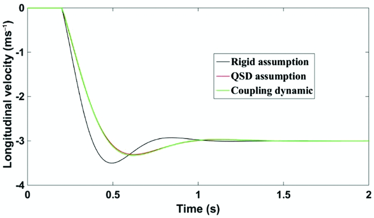
Figure 21 demonstrates the dynamic response of the prototype after a sharp-edged, longitudinal gust input, with a velocity of 3 ms−1. The airspeed of the prototype is 15 ms−1 (cruise speed). Three lines represent the response of the rigid model, coupling model, and QSD model, respectively. The figure shows that the response of the bio-inspired wing aircraft has a lower velocity change, a lower overshoot, and a shorter stabilisation time than the rigid response. This shows that the elasticity of the wing has considerable potential to change and optimise the flight dynamic characteristics and alleviate the gust response. The response of the dynamic coupling model and the QSD model are almost identical because of the frequency gap.

Figure 21. Vertical gust response of the prototype with an optimised wing.
Figure 22 presents the gust response of the prototype with the two different types of wings presented in Fig. 2. Table 8 summarises the structural properties of both wings. The dynamic responses of the four longitudinal states are presented here. As the QSD model results are almost identical with the results from the coupling dynamic model when the sign of C Q 1η1 is negative, only the QSD model was used for the following simulation. The results show that the forward arrangement of the inertial/elastic axis can make C Q 1η1 more negative, and efficiently alleviate gust perturbation by improving the longitudinal characteristics through aeroelastic coupling.
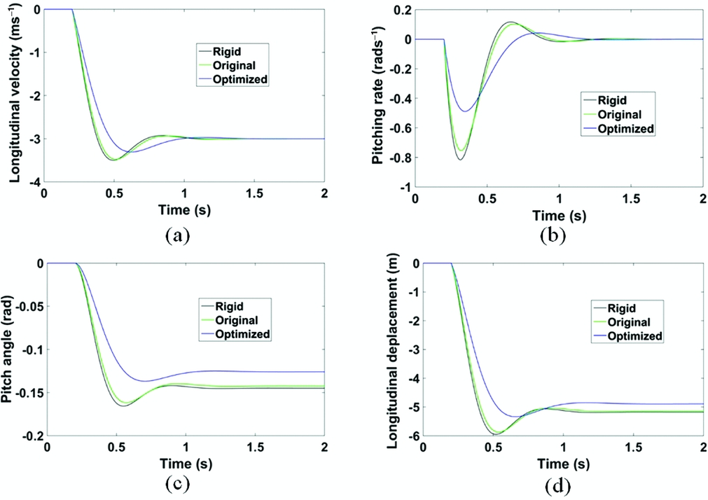
Figure 22. The gust response of different longitudinal flight dynamic states.
Table 8 Properties of the original wing and optimised wing in the simulation
Although there is no direct evidence to prove that this coupling effect does help birds to alleviate their gust response and strengthen their flight stability while they are gliding, this can be utilised on the alleviation of the small UAVs flying under low Reynold numbers, and be an alternative solution for the flight dynamic optimisation.
6.0 CONCLUSIONS
Three major features of a natural bird's wing were addressed in the design and optimisation of the bio-inspired wing and their specific effects on the coupling dynamics were analysed. The imitated rachis-barb structure can maintain the aerofoil shape; The thin aerofoil can significantly decrease the twisting stiffness of the wing. Thus, the first several structural modes of the wing all have twisting dominated mode shapes, making their first several aeroelastic mode frequencies much more sensitive to aerodynamics. The position of the inertial/elastic axis determinates whether the frequency will become larger or smaller when the airspeed increases. A forward axis position can make it increase, and a backward one can decrease it.
The first aeroelastic mode may affect the short period feature even if there is a considerable frequency gap between them. The rapidly increasing 1st aeroelastic mode frequency can decrease the frequency of the short period and increase its damping. The twisting dominated nature of the 1st mode can induce this effect significantly even at a pretty low airspeed. In some cases, the rapidly decreasing frequency can diminish the frequency gap and the first aeroelastic mode and the short period mode can couple strongly and lead to a body-freedom flutter phenomenon. In some other cases, the forward location of the inertial axis and elastic axis will make the natural frequency increase with increasing airspeed, making the short period more stable and less sensitive to the gust perturbance.
The coupling mechanisms of the bio-inspired membrane wing can be utilised to extend the abilities of SUAVs. These membrane wings are lightweight and can optimise flight dynamic properties by imitating the structural/geometric characteristics of a bird's wing. The aeroelastic effects can be utilised to improve rather than limit flight if the elastic wing is designed appropriately.
APPENDIX A GEOMETRIC AND MECHANICAL PROPERTIES OF THE ELASTIC MEMBRANE WINGS
This appendix presents the detailed structural features and material information of the elastic membrane wings shown in Fig. 2. Figure A1 shows the wing structure at different aerofoil planes. Two basic types of materials are used here. The black parts shown in aerofoils (Reference Beard and McLain1)~(4) represent a kind of carbon-fiber composite material. Different layers of carbon fiber are stuck together by glue and then formed by high temperature. The membrane wing thickness is determined by the number of the layers. The fibers of adjacent layers are oriented so that their directions are perpendicular with each other, allowing the membrane to present isotropic mechanical properties. The yellow parts shown in aerofoils (Reference Chabot and Bird3) and (Reference Videler4) of Fig. A1 represent a type of Kevlar-fiber material. Compared with the carbon-fiber composite, this material has lower stiffness and lower density. The Kevlar membrane is very thin (0.15~0.2 mm) and can be placed between two carbon-fiber layers. The use of this kind of material on the parts near the tailing edge can effectively adjust the inertial axis and the elastic axis toward the leading edge (shown in Fig. A2). Table A1 presents the mechanical properties of the two kinds of materials in detail.
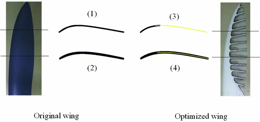
Figure A1. Membrane wing structure at different aerofoil planes.
Table A1 Mechanical properties of the materials
Figure A2. The location the of inertial axis and elastic axis.
APPENDIX B DETAILED FORMULATION OF THE COUPLING DYNAMIC MODEL
Detailed formulation of Equation (4):
 $$\begin{equation*}
{A_{RR}} = \left[ {\begin{array}{l@{\quad}c@{\quad}c@{\quad}c} {{X_u}}&{{X_\alpha }}&0&{ - g}\\ {{Z_u}/{u_0}}&{{Z_\alpha }/{u_0}}&1&0\\ {{M_u} + {M_{\dot{w}}}{Z_u}}&{{M_\alpha } + {M_{\dot{w}}}{Z_\alpha }}&{{M_q} + {M_{\dot{w}}}{u_0}}&0\\[6pt] 0&0&1&0 \end{array}} \right],
\end{equation*}$$
$$\begin{equation*}
{A_{RR}} = \left[ {\begin{array}{l@{\quad}c@{\quad}c@{\quad}c} {{X_u}}&{{X_\alpha }}&0&{ - g}\\ {{Z_u}/{u_0}}&{{Z_\alpha }/{u_0}}&1&0\\ {{M_u} + {M_{\dot{w}}}{Z_u}}&{{M_\alpha } + {M_{\dot{w}}}{Z_\alpha }}&{{M_q} + {M_{\dot{w}}}{u_0}}&0\\[6pt] 0&0&1&0 \end{array}} \right],
\end{equation*}$$
 $$\begin{eqnarray*}
{A_{RE}} &=& \left[ {\begin{array}{l@{\quad}c@{\quad}c} {{X_{{\eta _1}}}}&{...}&{{X_{{\eta _n}}}}\\ {{Z_{{\eta _1}}}/{u_0}}&{...}&{{Z_{{\eta _n}}}/{u_0}}\\ {{M_{{\eta _1}}} + {M_{\dot{w}}}{Z_{{\eta _1}}}}&{...}&{{M_{{\eta _n}}} + {M_{\dot{w}}}{Z_{{\eta _n}}}}\\ 0&{...}&0 \end{array}} \right],\nonumber\\
{A_{R\dot{E}}} &=& \left[ {\begin{array}{l@{\quad}c@{\quad}c} {{X_{{{\dot{\eta }}_1}}}}&{...}&{{X_{{{\dot{\eta }}_n}}}}\\ {{Z_{{{\dot{\eta }}_1}}}/{u_0}}&{...}&{{Z_{{{\dot{\eta }}_n}}}/{u_0}}\\ {{M_{{{\dot{\eta }}_1}}} + {M_{\dot{w}}}{Z_{{{\dot{\eta }}_1}}}}&{...}&{{M_{{{\dot{\eta }}_n}}} + {M_{\dot{w}}}{Z_{{{\dot{\eta }}_n}}}}\\ 0&{...}&0 \end{array}} \right]
\end{eqnarray*}$$
$$\begin{eqnarray*}
{A_{RE}} &=& \left[ {\begin{array}{l@{\quad}c@{\quad}c} {{X_{{\eta _1}}}}&{...}&{{X_{{\eta _n}}}}\\ {{Z_{{\eta _1}}}/{u_0}}&{...}&{{Z_{{\eta _n}}}/{u_0}}\\ {{M_{{\eta _1}}} + {M_{\dot{w}}}{Z_{{\eta _1}}}}&{...}&{{M_{{\eta _n}}} + {M_{\dot{w}}}{Z_{{\eta _n}}}}\\ 0&{...}&0 \end{array}} \right],\nonumber\\
{A_{R\dot{E}}} &=& \left[ {\begin{array}{l@{\quad}c@{\quad}c} {{X_{{{\dot{\eta }}_1}}}}&{...}&{{X_{{{\dot{\eta }}_n}}}}\\ {{Z_{{{\dot{\eta }}_1}}}/{u_0}}&{...}&{{Z_{{{\dot{\eta }}_n}}}/{u_0}}\\ {{M_{{{\dot{\eta }}_1}}} + {M_{\dot{w}}}{Z_{{{\dot{\eta }}_1}}}}&{...}&{{M_{{{\dot{\eta }}_n}}} + {M_{\dot{w}}}{Z_{{{\dot{\eta }}_n}}}}\\ 0&{...}&0 \end{array}} \right]
\end{eqnarray*}$$
 $$\begin{equation*}
{A_{ER}} = \left[ {\begin{array}{@{}*{4}{c}@{}} {{H_{1u}}}&{{H_{1\alpha }}}&{{H_{1q}}}&0\\ {...}&{...}&{...}&{...}\\ {{H_{nu}}}&{{H_{n\alpha }}}&{{H_{nq}}}&0 \end{array}} \right],{A_{EE}} = \left[ {\begin{array}{@{}*{4}{c}@{}} { - {\omega _1}^2{\rm{ + }}{H_{1{\eta _1}}}}&{{H_{1{\eta _2}}}}&{...}&{{H_{1{\eta _n}}}}\\ {{H_{2{\eta _1}}}}&{ - {\omega _2}^2{\rm{ + }}{H_{2{\eta _2}}}}&{...}&{{H_{2{\eta _n}}}}\\ {...}&{...}&{...}&{...}\\ {{H_{n{\eta _1}}}}&{{H_{n{\eta _2}}}}&{...}&{ - {\omega _n}^2{\rm{ + }}{H_{n{\eta _n}}}} \end{array}} \right]
\end{equation*}$$
$$\begin{equation*}
{A_{ER}} = \left[ {\begin{array}{@{}*{4}{c}@{}} {{H_{1u}}}&{{H_{1\alpha }}}&{{H_{1q}}}&0\\ {...}&{...}&{...}&{...}\\ {{H_{nu}}}&{{H_{n\alpha }}}&{{H_{nq}}}&0 \end{array}} \right],{A_{EE}} = \left[ {\begin{array}{@{}*{4}{c}@{}} { - {\omega _1}^2{\rm{ + }}{H_{1{\eta _1}}}}&{{H_{1{\eta _2}}}}&{...}&{{H_{1{\eta _n}}}}\\ {{H_{2{\eta _1}}}}&{ - {\omega _2}^2{\rm{ + }}{H_{2{\eta _2}}}}&{...}&{{H_{2{\eta _n}}}}\\ {...}&{...}&{...}&{...}\\ {{H_{n{\eta _1}}}}&{{H_{n{\eta _2}}}}&{...}&{ - {\omega _n}^2{\rm{ + }}{H_{n{\eta _n}}}} \end{array}} \right]
\end{equation*}$$
 $$\begin{equation*}
{A_{E\dot{E}}} = \left[ {\begin{array}{l@{\quad}c@{\quad}c@{\quad}c} { - {\zeta _1}{\omega _1}{\rm{ + }}{H_{1{{\dot{\eta }}_1}}}}&{{H_{1{{\dot{\eta }}_2}}}}&{...}&{{H_{1{{\dot{\eta }}_n}}}}\\ {{H_{2{{\dot{\eta }}_1}}}}&{ - {\zeta _2}{\omega _2}{\rm{ + }}{H_{2{{\dot{\eta }}_2}}}}&{...}&{{H_{2{{\dot{\eta }}_n}}}}\\ {...}&{...}&{...}&{...}\\ {{H_{n{{\dot{\eta }}_1}}}}&{{H_{n{{\dot{\eta }}_2}}}}&{...}&{ - {\zeta _n}{\omega _n}{\rm{ + }}{H_{n{{\dot{\eta }}_n}}}} \end{array}} \right]
\end{equation*}$$
$$\begin{equation*}
{A_{E\dot{E}}} = \left[ {\begin{array}{l@{\quad}c@{\quad}c@{\quad}c} { - {\zeta _1}{\omega _1}{\rm{ + }}{H_{1{{\dot{\eta }}_1}}}}&{{H_{1{{\dot{\eta }}_2}}}}&{...}&{{H_{1{{\dot{\eta }}_n}}}}\\ {{H_{2{{\dot{\eta }}_1}}}}&{ - {\zeta _2}{\omega _2}{\rm{ + }}{H_{2{{\dot{\eta }}_2}}}}&{...}&{{H_{2{{\dot{\eta }}_n}}}}\\ {...}&{...}&{...}&{...}\\ {{H_{n{{\dot{\eta }}_1}}}}&{{H_{n{{\dot{\eta }}_2}}}}&{...}&{ - {\zeta _n}{\omega _n}{\rm{ + }}{H_{n{{\dot{\eta }}_n}}}} \end{array}} \right]
\end{equation*}$$
 $$\begin{eqnarray*}
{G_R} &=& {\left[ {\begin{array}{*{20}{c}} {{X_\alpha }}&{{Z_\alpha }/{u_0}}&{{M_\alpha } + {M_{\dot{w}}}{Z_\alpha }}&0 \end{array}} \right]^T}/{u_0},\nonumber\\
{G_E} &=& {\left[ {\begin{array}{*{20}{c}} {{H_{1\alpha }}}&{...}&{{H_{n\alpha }}} \end{array}} \right]^T}/{u_0} \end{eqnarray*}$$
$$\begin{eqnarray*}
{G_R} &=& {\left[ {\begin{array}{*{20}{c}} {{X_\alpha }}&{{Z_\alpha }/{u_0}}&{{M_\alpha } + {M_{\dot{w}}}{Z_\alpha }}&0 \end{array}} \right]^T}/{u_0},\nonumber\\
{G_E} &=& {\left[ {\begin{array}{*{20}{c}} {{H_{1\alpha }}}&{...}&{{H_{n\alpha }}} \end{array}} \right]^T}/{u_0} \end{eqnarray*}$$
Table B1 Definition of aerodynamic derivatives about structural modes

Table B2 Definitions of derivatives in matrices A and G