


1 Introduction
Colloids immersed in electrolyte solutions usually carry net charges on their surface, which is further surrounded by a cloud of counterions. This cloud, as sketched in figure 1(a), is called the ‘electric double layer’ (EDL) and charged with more counterions than coions. Its typical thickness, also referred as the Debye length, is denoted by
 $\unicode[STIX]{x1D705}^{-1}$
, which is most commonly on the scale of 1–10 nm in water or fluids with high dielectric constants.
$\unicode[STIX]{x1D705}^{-1}$
, which is most commonly on the scale of 1–10 nm in water or fluids with high dielectric constants.

Figure 1. (a) Electric double layer (EDL): the ratio of the number of water molecules to that of the ions is exaggerated. The former is usually several orders of magnitude higher than the latter in a dilute solution. (b) Mechanism of diffusiophoresis when there is an external concentration gradient
 $\unicode[STIX]{x1D735}c_{\infty }$
. The dotted line indicates the EDL around the colloid. The solid and dotted arrows indicate the directions of the chemi-osmotic flow (COF) and the electro-osmotic flow (EOF), respectively. As a consequence, the velocity of the colloid (
$\unicode[STIX]{x1D735}c_{\infty }$
. The dotted line indicates the EDL around the colloid. The solid and dotted arrows indicate the directions of the chemi-osmotic flow (COF) and the electro-osmotic flow (EOF), respectively. As a consequence, the velocity of the colloid (
 $-\boldsymbol{u}_{d}$
) is in the opposite direction in the laboratory frame.
$-\boldsymbol{u}_{d}$
) is in the opposite direction in the laboratory frame.
If the electrolyte solution has a uniform concentration gradient
 $\unicode[STIX]{x1D735}c_{\infty }$
, the ion diffusion fluxes
$\unicode[STIX]{x1D735}c_{\infty }$
, the ion diffusion fluxes
 $\boldsymbol{j}_{+,D}=-D_{+}\unicode[STIX]{x1D735}c_{\infty }$
and
$\boldsymbol{j}_{+,D}=-D_{+}\unicode[STIX]{x1D735}c_{\infty }$
and
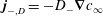 $\boldsymbol{j}_{-,D}=-D_{-}\unicode[STIX]{x1D735}c_{\infty }$
will be different due to differences between the diffusion coefficients of cations (
$\boldsymbol{j}_{-,D}=-D_{-}\unicode[STIX]{x1D735}c_{\infty }$
will be different due to differences between the diffusion coefficients of cations (
 $D_{+}$
) and anions (
$D_{+}$
) and anions (
 $D_{-}$
). Thus, an electric field
$D_{-}$
). Thus, an electric field
 $\boldsymbol{E}_{\infty }$
, which accelerates the slowly diffusing ions and decelerates the fast diffusing ions, will build up to maintain the electroneutrality in solution (Prieve et al.
Reference Prieve, Anderson, Ebel and Lowell1984), as shown in figure 1(b). The electric field causes motion of the suspended charged colloids by exerting a force on the fluid inside the EDL, which is the response known as electrophoresis. The solute gradient within the EDL also produces a pressure-driven osmotic flow, which is known as chemiphoresis. The direction of the electro-osmotic flow (EOF) depends on the electric field
$\boldsymbol{E}_{\infty }$
, which accelerates the slowly diffusing ions and decelerates the fast diffusing ions, will build up to maintain the electroneutrality in solution (Prieve et al.
Reference Prieve, Anderson, Ebel and Lowell1984), as shown in figure 1(b). The electric field causes motion of the suspended charged colloids by exerting a force on the fluid inside the EDL, which is the response known as electrophoresis. The solute gradient within the EDL also produces a pressure-driven osmotic flow, which is known as chemiphoresis. The direction of the electro-osmotic flow (EOF) depends on the electric field
 $\boldsymbol{E}_{\infty }$
and the charge on the particle/drop surface, while the direction of the chemi-osmotic flow (COF) is always from regions of high-to-low concentration (Prieve et al.
Reference Prieve, Anderson, Ebel and Lowell1984; Khair & Squires Reference Khair and Squires2009). The interplay of these two forces sets the particle velocity relative to the fluid, i.e.
$\boldsymbol{E}_{\infty }$
and the charge on the particle/drop surface, while the direction of the chemi-osmotic flow (COF) is always from regions of high-to-low concentration (Prieve et al.
Reference Prieve, Anderson, Ebel and Lowell1984; Khair & Squires Reference Khair and Squires2009). The interplay of these two forces sets the particle velocity relative to the fluid, i.e.
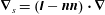
 $\boldsymbol{v}_{p}-\boldsymbol{v}_{f}=-\boldsymbol{u}_{d}$
, where
$\boldsymbol{v}_{p}-\boldsymbol{v}_{f}=-\boldsymbol{u}_{d}$
, where
 $\boldsymbol{v}_{p}$
,
$\boldsymbol{v}_{p}$
,
 $\boldsymbol{v}_{f}$
and
$\boldsymbol{v}_{f}$
and
 $-\boldsymbol{u}_{d}$
are the particle, local fluid and diffusiophoretic velocity of the particle, respectively.
$-\boldsymbol{u}_{d}$
are the particle, local fluid and diffusiophoretic velocity of the particle, respectively.
This mechanism of particle transport, induced by a concentration gradient and consisting of both the electrophoresis and chemiphoresis contributions, is called ‘diffusiophoresis’, first proposed by Derjaguin et al. (Reference Derjaguin, Sidorenkov, Zubashchenkov and Kiseleva1947) and Derjaguin et al. (Reference Derjaguin, Dukhin and Korotkova1961). Most of the previous studies of diffusiophoresis are limited to the motion of rigid particles (Prieve et al.
Reference Prieve, Anderson, Ebel and Lowell1984; Prieve & Roman Reference Prieve and Roman1987; Anderson Reference Anderson1989). The viscosity ratio
 $\overline{\unicode[STIX]{x1D707}}/\unicode[STIX]{x1D707}$
of a drop with viscosity
$\overline{\unicode[STIX]{x1D707}}/\unicode[STIX]{x1D707}$
of a drop with viscosity
 $\overline{\unicode[STIX]{x1D707}}$
and an outer solution with viscosity
$\overline{\unicode[STIX]{x1D707}}$
and an outer solution with viscosity
 $\unicode[STIX]{x1D707}$
is a key factor in the study of diffusiophoresis of drops; a rigid particle is a special case where
$\unicode[STIX]{x1D707}$
is a key factor in the study of diffusiophoresis of drops; a rigid particle is a special case where
 $\overline{\unicode[STIX]{x1D707}}/\unicode[STIX]{x1D707}\rightarrow \infty$
. In the literature, there are only a few papers studying the diffusiophoresis and electrophoresis of drops but they report different results concerning the dependence of the diffusiophoretic speed on
$\overline{\unicode[STIX]{x1D707}}/\unicode[STIX]{x1D707}\rightarrow \infty$
. In the literature, there are only a few papers studying the diffusiophoresis and electrophoresis of drops but they report different results concerning the dependence of the diffusiophoretic speed on
 $\overline{\unicode[STIX]{x1D707}}/\unicode[STIX]{x1D707}$
. For example, Baygents & Saville (Reference Baygents and Saville1988) calculate the diffusiophoretic speed with different
$\overline{\unicode[STIX]{x1D707}}/\unicode[STIX]{x1D707}$
. For example, Baygents & Saville (Reference Baygents and Saville1988) calculate the diffusiophoretic speed with different
 $\overline{\unicode[STIX]{x1D707}}/\unicode[STIX]{x1D707}$
, which disagrees the numerical results reported by Lou & Lee (Reference Lou and Lee2008). With respect to electrophoresis of droplets of radius
$\overline{\unicode[STIX]{x1D707}}/\unicode[STIX]{x1D707}$
, which disagrees the numerical results reported by Lou & Lee (Reference Lou and Lee2008). With respect to electrophoresis of droplets of radius
 $a$
, Booth (Reference Booth1951) and Jordan & Taylor (Reference Jordan and Taylor1952) give different dependence of droplet speed as a function of the imposed uniform electric field on
$a$
, Booth (Reference Booth1951) and Jordan & Taylor (Reference Jordan and Taylor1952) give different dependence of droplet speed as a function of the imposed uniform electric field on
 $\overline{\unicode[STIX]{x1D707}}/\unicode[STIX]{x1D707}$
in the limit
$\overline{\unicode[STIX]{x1D707}}/\unicode[STIX]{x1D707}$
in the limit
 $\unicode[STIX]{x1D706}=(\unicode[STIX]{x1D705}a)^{-1}\rightarrow 0$
. Additionally, Ohshima & Healy (Reference Ohshima and Healy1984) predict that the electrophoretic speed of a drop does not depend on
$\unicode[STIX]{x1D706}=(\unicode[STIX]{x1D705}a)^{-1}\rightarrow 0$
. Additionally, Ohshima & Healy (Reference Ohshima and Healy1984) predict that the electrophoretic speed of a drop does not depend on
 $\overline{\unicode[STIX]{x1D707}}/\unicode[STIX]{x1D707}$
when the zeta potential on the drop is very large and
$\overline{\unicode[STIX]{x1D707}}/\unicode[STIX]{x1D707}$
when the zeta potential on the drop is very large and
 $\unicode[STIX]{x1D706}$
is small, and they refer to this phenomenon as ‘solidification’ because the drop’s diffusiophoretic speed is the same as its equivalent solid particle (same size and zeta potential, but
$\unicode[STIX]{x1D706}$
is small, and they refer to this phenomenon as ‘solidification’ because the drop’s diffusiophoretic speed is the same as its equivalent solid particle (same size and zeta potential, but
 $\overline{\unicode[STIX]{x1D707}}/\unicode[STIX]{x1D707}\rightarrow \infty$
). However, numerical results reported by Baygents & Saville (Reference Baygents and Saville1991) show that the ‘solidification’ effects are more significant when
$\overline{\unicode[STIX]{x1D707}}/\unicode[STIX]{x1D707}\rightarrow \infty$
). However, numerical results reported by Baygents & Saville (Reference Baygents and Saville1991) show that the ‘solidification’ effects are more significant when
 $\unicode[STIX]{x1D706}$
increases. For bubbles, Schnitzer, Frankel & Yariv (Reference Schnitzer, Frankel and Yariv2014) reports an analysis of electrophoresis of bubbles but the theoretical results are at odds with the experimental observation.
$\unicode[STIX]{x1D706}$
increases. For bubbles, Schnitzer, Frankel & Yariv (Reference Schnitzer, Frankel and Yariv2014) reports an analysis of electrophoresis of bubbles but the theoretical results are at odds with the experimental observation.
In this paper, we investigate the diffusiophoresis of charged drops both analytically and experimentally. An analytical solution for the diffusiophoretic velocity of non-conductive drops, given in (2.66), is obtained using perturbation methods. In laboratory experiments, we use silicone oil droplets, which are charged by adding ionic surfactants, and measure their speed under a solute concentration gradient. The experiments show that the oil droplets move more slowly when
 $\overline{\unicode[STIX]{x1D707}}/\unicode[STIX]{x1D707}$
decreases. In particular, when the viscosity ratio (drop to continuous phase)
$\overline{\unicode[STIX]{x1D707}}/\unicode[STIX]{x1D707}$
decreases. In particular, when the viscosity ratio (drop to continuous phase)
 $\overline{\unicode[STIX]{x1D707}}/\unicode[STIX]{x1D707}>10$
, the diffusiophoretic speed of oil droplets is almost the same as their equivalent rigid-particle speed. The experimental results are in good agreement with our theory.
$\overline{\unicode[STIX]{x1D707}}/\unicode[STIX]{x1D707}>10$
, the diffusiophoretic speed of oil droplets is almost the same as their equivalent rigid-particle speed. The experimental results are in good agreement with our theory.
The applications of diffusiophoresis have been studied widely (Velegol et al. Reference Velegol, Garg, Guha, Kar and Kumar2016), but often restricted to solid particles, such as transport of colloids to/from a dead-end channel (Kar et al. Reference Kar, Chiang, Rivera, Sen and Velegol2015; Shin et al. Reference Shin, Um, Sabass, Ault, Rahimi, Warren and Stone2016), particle sorting and sample preconcentration (Shin et al. Reference Shin, Um, Sabass, Ault, Rahimi, Warren and Stone2016), water filtration and purification (Florea et al. Reference Florea, Musa, Huyghe and Wyss2014; Shin et al. Reference Shin, Shardt, Warren and Stone2017b ) and even detecting bone fractures (Yadav et al. Reference Yadav, Freedman, Grinstaff and Sen2013). Our theory can lay the foundation to extend these applications to droplets, such as is relevant for recovery of oil and drug delivery.
2 Modelling diffusiophoresis of a non-conductive drop
2.1 Model description
A spherical coordinate system
 $(r,\unicode[STIX]{x1D703})$
is fixed to the centre of a sphere of radius
$(r,\unicode[STIX]{x1D703})$
is fixed to the centre of a sphere of radius
 $a$
, axisymmetry is assumed and the flow velocity at infinity is denoted by
$a$
, axisymmetry is assumed and the flow velocity at infinity is denoted by
 $\boldsymbol{u}_{d}$
. The concentrations of the cations and anions are denoted
$\boldsymbol{u}_{d}$
. The concentrations of the cations and anions are denoted
 $c_{\pm }$
, respectively. For simplicity, the valences for both ions are assumed to be the same, denoted by
$c_{\pm }$
, respectively. For simplicity, the valences for both ions are assumed to be the same, denoted by
 $z$
, such as NaCl (where
$z$
, such as NaCl (where
 $z=1$
), KCl, etc. The direction of the concentration gradient is set to be aligned with the axis
$z=1$
), KCl, etc. The direction of the concentration gradient is set to be aligned with the axis
 $\unicode[STIX]{x1D703}=0$
, indicated by a unit vector
$\unicode[STIX]{x1D703}=0$
, indicated by a unit vector
 $\boldsymbol{e}_{x}$
, as shown in figure 2. Therefore, the uniform concentration gradient at
$\boldsymbol{e}_{x}$
, as shown in figure 2. Therefore, the uniform concentration gradient at
 $r\rightarrow \infty$
is
$r\rightarrow \infty$
is
 $\unicode[STIX]{x1D735}c_{\infty }=G\boldsymbol{e}_{x}$
, where
$\unicode[STIX]{x1D735}c_{\infty }=G\boldsymbol{e}_{x}$
, where
 $G$
is the magnitude. Due to symmetry, the direction of
$G$
is the magnitude. Due to symmetry, the direction of
 $\boldsymbol{u}_{d}$
should also be along
$\boldsymbol{u}_{d}$
should also be along
 $\boldsymbol{e}_{x}$
.
$\boldsymbol{e}_{x}$
.

Figure 2. (a) Model for a spherical drop: the particle surface is charged, either positively or negatively. The dotted line surrounding the particle represents the boundary layer. A spherical coordinate is fixed at the centre of the drop with the direction of
 $\unicode[STIX]{x1D703}=0$
, namely
$\unicode[STIX]{x1D703}=0$
, namely
 $\boldsymbol{e}_{x}$
, parallel to
$\boldsymbol{e}_{x}$
, parallel to
 $\unicode[STIX]{x1D735}c_{\infty }$
,
$\unicode[STIX]{x1D735}c_{\infty }$
,
 $\boldsymbol{u}_{d}$
and
$\boldsymbol{u}_{d}$
and
 $\boldsymbol{E}_{\infty }$
. Also,
$\boldsymbol{E}_{\infty }$
. Also,
 $\boldsymbol{n}$
is the unit normal vector at the interface. (b) The coordinate used in the boundary-layer solutions.
$\boldsymbol{n}$
is the unit normal vector at the interface. (b) The coordinate used in the boundary-layer solutions.
When the Debye length
 $\unicode[STIX]{x1D705}^{-1}$
is much smaller than the drop radius
$\unicode[STIX]{x1D705}^{-1}$
is much smaller than the drop radius
 $a$
, there is a boundary layer (i.e. the EDL) adjacent to the surface of the drop. The whole field is divided into three regions, namely the outer region outside the boundary layer in the bulk solution, the boundary layer adjacent to the drop surface in the continuous phase and the drop region inside the non-conductive drop, as labelled in figure 2(a). The corresponding analytical solutions in these regions are called the outer solution, boundary-layer solution and drop-region solution, respectively.
$a$
, there is a boundary layer (i.e. the EDL) adjacent to the surface of the drop. The whole field is divided into three regions, namely the outer region outside the boundary layer in the bulk solution, the boundary layer adjacent to the drop surface in the continuous phase and the drop region inside the non-conductive drop, as labelled in figure 2(a). The corresponding analytical solutions in these regions are called the outer solution, boundary-layer solution and drop-region solution, respectively.
2.2 Assumptions
The following assumptions are made in our modelling: (i) there is no solute in the drop; (ii)
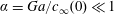 $\unicode[STIX]{x1D6FC}=Ga/c_{\infty }(0)\ll 1$
, where
$\unicode[STIX]{x1D6FC}=Ga/c_{\infty }(0)\ll 1$
, where
 $G$
is the magnitude of the imposed concentration gradient and
$G$
is the magnitude of the imposed concentration gradient and
 $c_{\infty }(0)$
is the solute concentration at
$c_{\infty }(0)$
is the solute concentration at
 $r=0$
in the absence of the particle, which is assumed to be known; (iii)
$r=0$
in the absence of the particle, which is assumed to be known; (iii)
 $\unicode[STIX]{x1D706}=(a\unicode[STIX]{x1D705})^{-1}\ll 1$
, where
$\unicode[STIX]{x1D706}=(a\unicode[STIX]{x1D705})^{-1}\ll 1$
, where
 $\unicode[STIX]{x1D705}^{-1}$
is the Debye length (defined precisely later). The first assumption has a wide application to water–oil systems, because oil is non-polar and most electrolytes dissolve sparingly in it. The second assumption implies that the concentration difference at the scale of the size of drop is much smaller than the background concentration. This limit can be achieved when either the concentration gradient or the size of droplet is sufficiently small. The third assumption requires the electric double layer thickness to be much smaller than the radius of droplet. A typical scale for the Debye length is approximately 1–10 nm in water or fluids with high dielectric constants. A droplet at the scale of
$\unicode[STIX]{x1D705}^{-1}$
is the Debye length (defined precisely later). The first assumption has a wide application to water–oil systems, because oil is non-polar and most electrolytes dissolve sparingly in it. The second assumption implies that the concentration difference at the scale of the size of drop is much smaller than the background concentration. This limit can be achieved when either the concentration gradient or the size of droplet is sufficiently small. The third assumption requires the electric double layer thickness to be much smaller than the radius of droplet. A typical scale for the Debye length is approximately 1–10 nm in water or fluids with high dielectric constants. A droplet at the scale of
 $1~\unicode[STIX]{x03BC}\text{m}$
or larger would typically satisfy
$1~\unicode[STIX]{x03BC}\text{m}$
or larger would typically satisfy
 $\unicode[STIX]{x1D706}\ll 1$
very well. In the following analysis, we first use a regular perturbation on
$\unicode[STIX]{x1D706}\ll 1$
very well. In the following analysis, we first use a regular perturbation on
 $\unicode[STIX]{x1D6FC}$
, then for each order of
$\unicode[STIX]{x1D6FC}$
, then for each order of
 $\unicode[STIX]{x1D6FC}$
, a singular perturbation on
$\unicode[STIX]{x1D6FC}$
, a singular perturbation on
 $\unicode[STIX]{x1D706}$
is further applied.
$\unicode[STIX]{x1D706}$
is further applied.
2.3 Governing equations and boundary conditions
The ion flux is
 $$\begin{eqnarray}\boldsymbol{j}_{\pm }=c_{\pm }\boldsymbol{u}-D_{\pm }\left(\unicode[STIX]{x1D735}c_{\pm }\pm \frac{zec_{\pm }}{k_{B}T}\unicode[STIX]{x1D735}\unicode[STIX]{x1D713}\right),\end{eqnarray}$$
where
 $c_{+}(c_{-})$
is the concentration of cations (anions),
$c_{+}(c_{-})$
is the concentration of cations (anions),
 $e$
is the elementary charge,
$e$
is the elementary charge,
 $\boldsymbol{u}$
is the velocity field,
$\boldsymbol{u}$
is the velocity field,
 $\unicode[STIX]{x1D713}$
is the electric potential,
$\unicode[STIX]{x1D713}$
is the electric potential,
 $k_{B}$
and
$k_{B}$
and
 $T$
are the Boltzmann constant and the temperature, respectively. Since the flow field
$T$
are the Boltzmann constant and the temperature, respectively. Since the flow field
 $\boldsymbol{u}$
is incompressible, the continuity of ions using (2.1) can be written as
$\boldsymbol{u}$
is incompressible, the continuity of ions using (2.1) can be written as
 $$\begin{eqnarray}D_{\pm }\unicode[STIX]{x1D735}\boldsymbol{\cdot }\left[\unicode[STIX]{x1D735}c_{\pm }\pm \frac{ze}{k_{B}T}c_{\pm }\unicode[STIX]{x1D735}\unicode[STIX]{x1D713}\right]=\boldsymbol{u}\boldsymbol{\cdot }\unicode[STIX]{x1D735}c_{\pm }+\frac{\unicode[STIX]{x2202}c_{\pm }}{\unicode[STIX]{x2202}t}.\end{eqnarray}$$
The governing equation for the electric potential
 $\unicode[STIX]{x1D713}$
, with electric field
$\unicode[STIX]{x1D713}$
, with electric field
 $\boldsymbol{E}=-\unicode[STIX]{x1D735}\unicode[STIX]{x1D713}$
, is Gauss’s law
$\boldsymbol{E}=-\unicode[STIX]{x1D735}\unicode[STIX]{x1D713}$
, is Gauss’s law
 $$\begin{eqnarray}\unicode[STIX]{x1D6FB}^{2}\unicode[STIX]{x1D713}=-\frac{\unicode[STIX]{x1D70C}_{e}}{\unicode[STIX]{x1D716}},\end{eqnarray}$$
where
 $\unicode[STIX]{x1D716}$
is the permittivity of the fluid and
$\unicode[STIX]{x1D716}$
is the permittivity of the fluid and
 $\unicode[STIX]{x1D70C}_{e}$
is the local charge density, i.e.
$\unicode[STIX]{x1D70C}_{e}$
is the local charge density, i.e.
 $$\begin{eqnarray}\unicode[STIX]{x1D70C}_{e}=ez(c_{+}-c_{-}).\end{eqnarray}$$
Finally, because the Reynolds number
 $Re$
is assumed small, the incompressible flow field is governed by the Stokes equations with an electric body force
$Re$
is assumed small, the incompressible flow field is governed by the Stokes equations with an electric body force
 $$\begin{eqnarray}\displaystyle & 0=-\unicode[STIX]{x1D735}p+\unicode[STIX]{x1D707}\unicode[STIX]{x1D6FB}^{2}\boldsymbol{u}-\unicode[STIX]{x1D70C}_{e}\unicode[STIX]{x1D735}\unicode[STIX]{x1D713}, & \displaystyle\end{eqnarray}$$
 $$\begin{eqnarray}\displaystyle & \unicode[STIX]{x1D735}\boldsymbol{\cdot }\boldsymbol{u}=0, & \displaystyle\end{eqnarray}$$
 $p$
is the pressure and
$p$
is the pressure and
 $\unicode[STIX]{x1D707}$
is the viscosity.
$\unicode[STIX]{x1D707}$
is the viscosity. The Newtonian stress and Maxwell stress tensors are denoted, respectively, by
 $\unicode[STIX]{x1D61A}_{N}$
and
$\unicode[STIX]{x1D61A}_{N}$
and
 $\unicode[STIX]{x1D61A}_{M}$
, namely
$\unicode[STIX]{x1D61A}_{M}$
, namely
 $$\begin{eqnarray}\displaystyle & \unicode[STIX]{x1D61A}_{N}=-p\unicode[STIX]{x1D644}+\unicode[STIX]{x1D707}(\unicode[STIX]{x1D735}\boldsymbol{u}+\unicode[STIX]{x1D735}\boldsymbol{u}^{\text{T}}), & \displaystyle\end{eqnarray}$$
 $$\begin{eqnarray}\displaystyle & \unicode[STIX]{x1D61A}_{M}=\unicode[STIX]{x1D716}\left[\unicode[STIX]{x1D735}\unicode[STIX]{x1D713}\unicode[STIX]{x1D735}\unicode[STIX]{x1D713}-{\textstyle \frac{1}{2}}(\unicode[STIX]{x1D735}\unicode[STIX]{x1D713}\boldsymbol{\cdot }\unicode[STIX]{x1D735}\unicode[STIX]{x1D713})\unicode[STIX]{x1D644}\right], & \displaystyle\end{eqnarray}$$
 $\unicode[STIX]{x1D644}$
is the identity tensor. We denote the fields inside the drop with an overbar. At the interface of the drop (
$\unicode[STIX]{x1D644}$
is the identity tensor. We denote the fields inside the drop with an overbar. At the interface of the drop (
 $r=a$
), we have continuity of velocity and a stress balance (Leal Reference Leal2007), i.e.
$r=a$
), we have continuity of velocity and a stress balance (Leal Reference Leal2007), i.e.  $$\begin{eqnarray}\displaystyle & \boldsymbol{u}=\overline{\boldsymbol{u}}, & \displaystyle\end{eqnarray}$$
 $$\begin{eqnarray}\displaystyle & \boldsymbol{n}\boldsymbol{\cdot }(\unicode[STIX]{x1D61A}_{N}+\unicode[STIX]{x1D61A}_{M})-\unicode[STIX]{x1D70E}(\unicode[STIX]{x1D735}_{\!s}\boldsymbol{\cdot }\boldsymbol{n})\boldsymbol{n}+\unicode[STIX]{x1D735}_{\!s}\unicode[STIX]{x1D70E}=\boldsymbol{n}\boldsymbol{\cdot }(\overline{\unicode[STIX]{x1D61A}}_{N}+\overline{\unicode[STIX]{x1D61A}}_{M}) & \displaystyle\end{eqnarray}$$
 $$\begin{eqnarray}\boldsymbol{n}\boldsymbol{\cdot }\boldsymbol{u}=0,\end{eqnarray}$$
where
 $\boldsymbol{n}$
is the unit normal vector at the interface pointing away from the drop into the bulk solution,
$\boldsymbol{n}$
is the unit normal vector at the interface pointing away from the drop into the bulk solution,
 $\unicode[STIX]{x1D70E}$
is the surface tension and
$\unicode[STIX]{x1D70E}$
is the surface tension and
 $\unicode[STIX]{x1D735}_{s}=\left(\unicode[STIX]{x1D644}-\boldsymbol{n}\boldsymbol{n}\right)\boldsymbol{\cdot }\unicode[STIX]{x1D735}$
is the gradient along the surface. We assume there is no surfactant gradient in the solution and thus no surface tension gradient, i.e.
$\unicode[STIX]{x1D735}_{s}=\left(\unicode[STIX]{x1D644}-\boldsymbol{n}\boldsymbol{n}\right)\boldsymbol{\cdot }\unicode[STIX]{x1D735}$
is the gradient along the surface. We assume there is no surfactant gradient in the solution and thus no surface tension gradient, i.e.
 $\unicode[STIX]{x1D735}_{\!s}\unicode[STIX]{x1D70E}=\mathbf{0}$
in (2.7). Also since there is no solute inside the droplet, the normal ion flux at the interface (
$\unicode[STIX]{x1D735}_{\!s}\unicode[STIX]{x1D70E}=\mathbf{0}$
in (2.7). Also since there is no solute inside the droplet, the normal ion flux at the interface (
 $r=a$
) should vanish, i.e.
$r=a$
) should vanish, i.e.
 $$\begin{eqnarray}\boldsymbol{n}\boldsymbol{\cdot }\boldsymbol{j}_{\pm }=0.\end{eqnarray}$$
The boundary conditions for the electric potential at
 $r=a$
are
$r=a$
are
 $$\begin{eqnarray}\displaystyle & \boldsymbol{n}\boldsymbol{\cdot }(\unicode[STIX]{x1D716}\unicode[STIX]{x1D735}\unicode[STIX]{x1D713}-\overline{\unicode[STIX]{x1D716}}\unicode[STIX]{x1D735}\overline{\unicode[STIX]{x1D713}})=f_{e}, & \displaystyle\end{eqnarray}$$
 $$\begin{eqnarray}\displaystyle & \unicode[STIX]{x1D735}_{s}\unicode[STIX]{x1D713}=\unicode[STIX]{x1D735}_{s}\overline{\unicode[STIX]{x1D713}}\quad \text{or}\quad \unicode[STIX]{x1D713}=\overline{\unicode[STIX]{x1D713}}, & \displaystyle\end{eqnarray}$$
 $f_{e}$
is the surface charge density and in (2.10b
) there is no loss of generality setting a constant of integration to be zero.
$f_{e}$
is the surface charge density and in (2.10b
) there is no loss of generality setting a constant of integration to be zero.The boundary condition for the concentration field far from the droplet is
 $$\begin{eqnarray}\unicode[STIX]{x1D735}c_{+}=\unicode[STIX]{x1D735}c_{-}\rightarrow \unicode[STIX]{x1D735}c_{\infty }=G\boldsymbol{e}_{x}\quad \text{as }r\rightarrow \infty .\end{eqnarray}$$
To maintain electroneutrality in the outer region, we should have
 $\boldsymbol{j}_{+}=\boldsymbol{j}_{-}$
, which gives
$\boldsymbol{j}_{+}=\boldsymbol{j}_{-}$
, which gives
 $$\begin{eqnarray}c_{+}\boldsymbol{u}-D_{+}\left(\unicode[STIX]{x1D735}c_{+}+\frac{zec_{+}}{k_{B}T}\unicode[STIX]{x1D735}\unicode[STIX]{x1D713}_{\infty }\right)=c_{-}\boldsymbol{u}-D_{-}\left(\unicode[STIX]{x1D735}c_{-}-\frac{zec_{-}}{k_{B}T}\unicode[STIX]{x1D735}\unicode[STIX]{x1D713}_{\infty }\right).\end{eqnarray}$$
Thus, as
 $r\rightarrow \infty$
, in accordance with (2.11), equation (2.12) leads to
$r\rightarrow \infty$
, in accordance with (2.11), equation (2.12) leads to
 $$\begin{eqnarray}\boldsymbol{E}_{\infty }=-\unicode[STIX]{x1D735}\unicode[STIX]{x1D713}_{\infty }=\frac{k_{B}T}{ze}\unicode[STIX]{x1D6FD}\unicode[STIX]{x1D735}\ln c_{\infty },\end{eqnarray}$$
where
 $$\begin{eqnarray}\unicode[STIX]{x1D6FD}=\frac{D_{+}-D_{-}}{D_{+}+D_{-}}.\end{eqnarray}$$
Equation (2.13), together with (2.14), is a classical result derived in Prieve et al. (Reference Prieve, Anderson, Ebel and Lowell1984). It serves as the boundary condition for the electric field at
 $r\rightarrow \infty$
, and explicitly shows how the presence of an ion concentration gradient and a difference of cation and anion diffusivities give rise to a local electric field.
$r\rightarrow \infty$
, and explicitly shows how the presence of an ion concentration gradient and a difference of cation and anion diffusivities give rise to a local electric field.
2.4 Scaling
The drop radius
 $a$
is chosen as the typical length scale, so we define
$a$
is chosen as the typical length scale, so we define
 $R=r/a$
and the dimensionless gradient operator
$R=r/a$
and the dimensionless gradient operator
 $\widetilde{\unicode[STIX]{x1D735}}=a\unicode[STIX]{x1D735}$
. Equation (2.2) gives
$\widetilde{\unicode[STIX]{x1D735}}=a\unicode[STIX]{x1D735}$
. Equation (2.2) gives
 $\unicode[STIX]{x1D713}=O(k_{B}T/ze)$
. In (2.5a
), we have
$\unicode[STIX]{x1D713}=O(k_{B}T/ze)$
. In (2.5a
), we have
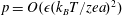 $p=O(\unicode[STIX]{x1D716}(k_{B}T/zea)^{2})$
using (2.3) to recognize
$p=O(\unicode[STIX]{x1D716}(k_{B}T/zea)^{2})$
using (2.3) to recognize
 $\unicode[STIX]{x1D70C}_{e}=O(\unicode[STIX]{x1D716}k_{B}T/zea^{2})$
and also
$\unicode[STIX]{x1D70C}_{e}=O(\unicode[STIX]{x1D716}k_{B}T/zea^{2})$
and also
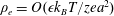
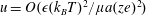 $u=O(\unicode[STIX]{x1D716}(k_{B}T)^{2}/\unicode[STIX]{x1D707}a(ze)^{2})$
. In (2.7), the surface tension is scaled with
$u=O(\unicode[STIX]{x1D716}(k_{B}T)^{2}/\unicode[STIX]{x1D707}a(ze)^{2})$
. In (2.7), the surface tension is scaled with
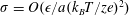 $\unicode[STIX]{x1D70E}=O(\unicode[STIX]{x1D716}/a(k_{B}T/ze)^{2})$
and the dimensionless surface tension is denoted by
$\unicode[STIX]{x1D70E}=O(\unicode[STIX]{x1D716}/a(k_{B}T/ze)^{2})$
and the dimensionless surface tension is denoted by
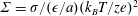 $\unicode[STIX]{x1D6F4}=\unicode[STIX]{x1D70E}/(\unicode[STIX]{x1D716}/a)(k_{B}T/ze)^{2}$
. In particular, it is useful to note that diffusiophoresis is driven by a concentration gradient, equation (2.11), which in dimensionless terms is
$\unicode[STIX]{x1D6F4}=\unicode[STIX]{x1D70E}/(\unicode[STIX]{x1D716}/a)(k_{B}T/ze)^{2}$
. In particular, it is useful to note that diffusiophoresis is driven by a concentration gradient, equation (2.11), which in dimensionless terms is
 $O(\unicode[STIX]{x1D6FC})$
. Recalling that
$O(\unicode[STIX]{x1D6FC})$
. Recalling that
 $\unicode[STIX]{x1D6FC}=Ga/c_{\infty }\ll 1$
, we now assume a regular perturbation series in
$\unicode[STIX]{x1D6FC}=Ga/c_{\infty }\ll 1$
, we now assume a regular perturbation series in
 $\unicode[STIX]{x1D6FC}$
, i.e.
$\unicode[STIX]{x1D6FC}$
, i.e.
 $$\begin{eqnarray}\displaystyle & c_{\pm }=c_{\infty }(0)(C_{0\pm }+\unicode[STIX]{x1D6FC}C_{1\pm }+O(\unicode[STIX]{x1D6FC}^{2})), & \displaystyle\end{eqnarray}$$
 $$\begin{eqnarray}\displaystyle & \unicode[STIX]{x1D713}={\displaystyle \frac{k_{B}T}{ze}}(\unicode[STIX]{x1D6F9}_{0}+\unicode[STIX]{x1D6FC}\unicode[STIX]{x1D6F9}_{1}+O(\unicode[STIX]{x1D6FC}^{2})), & \displaystyle\end{eqnarray}$$
 $$\begin{eqnarray}\displaystyle & \displaystyle \boldsymbol{u}={\displaystyle \frac{\unicode[STIX]{x1D716}(k_{B}T)^{2}}{\unicode[STIX]{x1D707}a(ze)^{2}}}(0+\unicode[STIX]{x1D6FC}\boldsymbol{U}_{1}+O(\unicode[STIX]{x1D6FC}^{2}))={\displaystyle \frac{\unicode[STIX]{x1D6FC}\unicode[STIX]{x1D716}(k_{B}T)^{2}}{\unicode[STIX]{x1D707}a(ze)^{2}}}\boldsymbol{U}_{1}+O(\unicode[STIX]{x1D6FC}^{2}), & \displaystyle\end{eqnarray}$$
 $$\begin{eqnarray}\displaystyle & \displaystyle p=\unicode[STIX]{x1D716}\left({\displaystyle \frac{k_{B}T}{zea}}\right)^{2}(P_{0}+\unicode[STIX]{x1D6FC}P_{1}+O(\unicode[STIX]{x1D6FC}^{2})). & \displaystyle\end{eqnarray}$$
 $f_{e}$
can be non-dimensionalized by
$f_{e}$
can be non-dimensionalized by
 $zec_{\infty }(0)a$
, and expanded as
$zec_{\infty }(0)a$
, and expanded as  $$\begin{eqnarray}f_{e}=zec_{\infty }(0)a(F_{0}+\unicode[STIX]{x1D6FC}F_{1}+O(\unicode[STIX]{x1D6FC}^{2})).\end{eqnarray}$$
With this notation, the capital letters are non-dimensionalized with the subscript indicating the order of
 $\unicode[STIX]{x1D6FC}$
. Note that
$\unicode[STIX]{x1D6FC}$
. Note that
 $\boldsymbol{U}_{0}=\mathbf{0}$
in (2.15c
) because the flow field is induced by the concentration gradient. Also, the contribution of the deformation of a spherical drop to its velocity is
$\boldsymbol{U}_{0}=\mathbf{0}$
in (2.15c
) because the flow field is induced by the concentration gradient. Also, the contribution of the deformation of a spherical drop to its velocity is
 $O(\unicode[STIX]{x1D716}E^{2}a/\unicode[STIX]{x1D70E})$
(Mandal, Bandopadhyay & Chakraborty Reference Mandal, Bandopadhyay and Chakraborty2016), which is the electric capillary number. With the orders of magnitude indicated in (2.15), the electric capillary number is
$O(\unicode[STIX]{x1D716}E^{2}a/\unicode[STIX]{x1D70E})$
(Mandal, Bandopadhyay & Chakraborty Reference Mandal, Bandopadhyay and Chakraborty2016), which is the electric capillary number. With the orders of magnitude indicated in (2.15), the electric capillary number is
 $\unicode[STIX]{x1D6FC}\unicode[STIX]{x1D716}/a\unicode[STIX]{x1D70E}(k_{B}T/ze)^{2}\ll 1$
(for silicone oil droplets with radius
$\unicode[STIX]{x1D6FC}\unicode[STIX]{x1D716}/a\unicode[STIX]{x1D70E}(k_{B}T/ze)^{2}\ll 1$
(for silicone oil droplets with radius
 $1~\unicode[STIX]{x03BC}\text{m}$
in water at room temperature,
$1~\unicode[STIX]{x03BC}\text{m}$
in water at room temperature,
 $\unicode[STIX]{x1D716}/a\unicode[STIX]{x1D70E}(k_{B}T/ze)^{2}=O(10^{-5})$
). Thus, the deformation of the drop can be neglected.
$\unicode[STIX]{x1D716}/a\unicode[STIX]{x1D70E}(k_{B}T/ze)^{2}=O(10^{-5})$
). Thus, the deformation of the drop can be neglected.
In the following analysis, we use both a regular perturbation on
 $\unicode[STIX]{x1D6FC}$
, as above, and a singular perturbation on
$\unicode[STIX]{x1D6FC}$
, as above, and a singular perturbation on
 $\unicode[STIX]{x1D706}=(a\unicode[STIX]{x1D705})^{-1}\ll 1$
to solve the governing equations. For example, as shown in (2.33) below, the
$\unicode[STIX]{x1D706}=(a\unicode[STIX]{x1D705})^{-1}\ll 1$
to solve the governing equations. For example, as shown in (2.33) below, the
 $O(\unicode[STIX]{x1D6FC}^{0})$
for the electric potential
$O(\unicode[STIX]{x1D6FC}^{0})$
for the electric potential
 $\unicode[STIX]{x1D6F9}$
can be further expanded as a series of
$\unicode[STIX]{x1D6F9}$
can be further expanded as a series of
 $\unicode[STIX]{x1D706}$
, i.e.
$\unicode[STIX]{x1D706}$
, i.e.
 $$\begin{eqnarray}\unicode[STIX]{x1D6F9}_{0}=\unicode[STIX]{x1D6F9}_{0}^{(0)}+\unicode[STIX]{x1D706}\unicode[STIX]{x1D6F9}_{0}^{(1)}+O(\unicode[STIX]{x1D706}^{2}),\end{eqnarray}$$
where the superscript ‘
 $n$
’ indicates the order of expansion in
$n$
’ indicates the order of expansion in
 $\unicode[STIX]{x1D706}$
(and the subscript is the order of expansion in
$\unicode[STIX]{x1D706}$
(and the subscript is the order of expansion in
 $\unicode[STIX]{x1D6FC}$
). This expansion in
$\unicode[STIX]{x1D6FC}$
). This expansion in
 $\unicode[STIX]{x1D706}$
can be similarly applied to any field variable at any order of
$\unicode[STIX]{x1D706}$
can be similarly applied to any field variable at any order of
 $\unicode[STIX]{x1D6FC}$
. We next construct solutions to the governing equations.
$\unicode[STIX]{x1D6FC}$
. We next construct solutions to the governing equations.
2.5
 $O(\unicode[STIX]{x1D6FC}^{0})$
and
$O(\unicode[STIX]{x1D6FC},\unicode[STIX]{x1D706}^{0})$
outer solutions of the concentration and electric fields
$O(\unicode[STIX]{x1D6FC}^{0})$
and
$O(\unicode[STIX]{x1D6FC},\unicode[STIX]{x1D706}^{0})$
outer solutions of the concentration and electric fields


The
 $O(\unicode[STIX]{x1D6FC}^{0})$
of both the concentration field and electric potential are constant in the absence of the particle and the concentration gradient. The constant concentration field is
$O(\unicode[STIX]{x1D6FC}^{0})$
of both the concentration field and electric potential are constant in the absence of the particle and the concentration gradient. The constant concentration field is
 $c_{\infty }(0)$
in dimensional form or
$c_{\infty }(0)$
in dimensional form or
 $1$
in dimensionless form, as shown in (2.15a
); the constant undisturbed electric potential is defined by
$1$
in dimensionless form, as shown in (2.15a
); the constant undisturbed electric potential is defined by
 $\unicode[STIX]{x1D6F9}_{\infty }(0)$
, i.e.
$\unicode[STIX]{x1D6F9}_{\infty }(0)$
, i.e.
 $$\begin{eqnarray}\displaystyle & C_{o,0+}=C_{o,0-}=C_{o,0}=1, & \displaystyle\end{eqnarray}$$
 $$\begin{eqnarray}\displaystyle & \unicode[STIX]{x1D6F9}_{o,0}=\unicode[STIX]{x1D6F9}_{\infty }(0), & \displaystyle\end{eqnarray}$$
 $o$
’ represents the outer solution and
$o$
’ represents the outer solution and
 $C_{o,0}$
is the concentration field for both cations and anions in the outer region at
$C_{o,0}$
is the concentration field for both cations and anions in the outer region at
 $O(\unicode[STIX]{x1D6FC}^{0})$
.
$O(\unicode[STIX]{x1D6FC}^{0})$
. At
 $O(\unicode[STIX]{x1D6FC})$
, there is no net charge in the outer region, therefore, the Poisson equation (2.3) becomes
$O(\unicode[STIX]{x1D6FC})$
, there is no net charge in the outer region, therefore, the Poisson equation (2.3) becomes
 $$\begin{eqnarray}\widetilde{\unicode[STIX]{x1D6FB}}^{2}\unicode[STIX]{x1D6F9}_{o,1}=0.\end{eqnarray}$$
The concentration field in the outer region should satisfy
 $$\begin{eqnarray}C_{o,1+}=C_{o,1-}=C_{o,1},\end{eqnarray}$$
where
 $C_{o,1}$
is the concentration field for both cations and anions in the outer region at
$C_{o,1}$
is the concentration field for both cations and anions in the outer region at
 $O(\unicode[STIX]{x1D6FC})$
. If we neglect the convective term in (2.2), the continuity of ions leads to
$O(\unicode[STIX]{x1D6FC})$
. If we neglect the convective term in (2.2), the continuity of ions leads to
 $$\begin{eqnarray}\displaystyle \widetilde{\unicode[STIX]{x1D6FB}}^{2}C_{o,1}=0. & & \displaystyle\end{eqnarray}$$
Neglecting the convection can be justified by assuming the Péclet number
 $Pe=ua/D\ll 1$
. Based on the scaling identified in § 2.4, the Péclet number is given by
$Pe=ua/D\ll 1$
. Based on the scaling identified in § 2.4, the Péclet number is given by
 $$\begin{eqnarray}Pe=\unicode[STIX]{x1D6FC}\frac{\unicode[STIX]{x1D716}(k_{B}T)^{2}}{\unicode[STIX]{x1D707}D^{\ast }(ze)^{2}},\end{eqnarray}$$
where we assume
 $D_{+}$
and
$D_{+}$
and
 $D_{-}$
are of the same order of magnitude, indicated by
$D_{-}$
are of the same order of magnitude, indicated by
 $D^{\ast }$
. An estimate for
$D^{\ast }$
. An estimate for
 $Pe/\unicode[STIX]{x1D6FC}$
using
$Pe/\unicode[STIX]{x1D6FC}$
using
 $D^{\ast }=10^{-9}~\text{m}^{2}~\text{s}^{-1}$
,
$D^{\ast }=10^{-9}~\text{m}^{2}~\text{s}^{-1}$
,
 $T=300~\text{K}$
and
$T=300~\text{K}$
and
 $z=1$
shows that
$z=1$
shows that
 $Pe/\unicode[STIX]{x1D6FC}\simeq 0.5$
for water. Thus, the convective term, as characterized by
$Pe/\unicode[STIX]{x1D6FC}\simeq 0.5$
for water. Thus, the convective term, as characterized by
 $Pe$
, for ion transport can be neglected when
$Pe$
, for ion transport can be neglected when
 $\unicode[STIX]{x1D6FC}\ll 1$
.
$\unicode[STIX]{x1D6FC}\ll 1$
.
By matching with (2.11), the boundary conditions for the concentration field in the outer region at
 $O(\unicode[STIX]{x1D6FC},\unicode[STIX]{x1D706}^{0})$
are
$O(\unicode[STIX]{x1D6FC},\unicode[STIX]{x1D706}^{0})$
are
 $$\begin{eqnarray}\displaystyle & \widetilde{\unicode[STIX]{x1D735}}C_{o,1}^{(0)}\rightarrow \boldsymbol{e}_{x}\quad \text{as }R\rightarrow \infty , & \displaystyle\end{eqnarray}$$
 $$\begin{eqnarray}\displaystyle & \boldsymbol{n}\boldsymbol{\cdot }\widetilde{\unicode[STIX]{x1D735}}C_{o,1}^{(0)}=0\quad \text{at }R=1^{+}, & \displaystyle\end{eqnarray}$$
 $R=1^{+}$
indicates the outer boundary of the EDL at the drop surface. We note that (2.23b
) is based on the assumption that there are no solutes inside the droplet and consequently the normal ion flux at the interface is
$R=1^{+}$
indicates the outer boundary of the EDL at the drop surface. We note that (2.23b
) is based on the assumption that there are no solutes inside the droplet and consequently the normal ion flux at the interface is
 $O(\unicode[STIX]{x1D706})$
(Anderson & Prieve Reference Anderson and Prieve1991; Pawar, Solomentsev & Anderson Reference Pawar, Solomentsev and Anderson1993). Therefore, in the limit
$O(\unicode[STIX]{x1D706})$
(Anderson & Prieve Reference Anderson and Prieve1991; Pawar, Solomentsev & Anderson Reference Pawar, Solomentsev and Anderson1993). Therefore, in the limit
 $\unicode[STIX]{x1D706}\rightarrow 0$
, the normal flux at the outer boundary of the EDL can be neglected. Also, up to
$\unicode[STIX]{x1D706}\rightarrow 0$
, the normal flux at the outer boundary of the EDL can be neglected. Also, up to
 $O(\unicode[STIX]{x1D706}^{0})$
,
$O(\unicode[STIX]{x1D706}^{0})$
,
 $R=1^{+}$
can be replaced by
$R=1^{+}$
can be replaced by
 $R=1$
in (2.23b
). With these assumptions, the solution of (2.21) with (2.23) is
$R=1$
in (2.23b
). With these assumptions, the solution of (2.21) with (2.23) is  $$\begin{eqnarray}C_{o,1}^{(0)}(R,\unicode[STIX]{x1D703})=\left(1+\frac{1}{2R^{3}}\right)\boldsymbol{R}\boldsymbol{\cdot }\boldsymbol{e}_{x}.\end{eqnarray}$$
This solution is the outer concentration field at
 $O(\unicode[STIX]{x1D6FC},\unicode[STIX]{x1D706}^{0})$
. Similarly the boundary conditions for the electric field in the outer region at
$O(\unicode[STIX]{x1D6FC},\unicode[STIX]{x1D706}^{0})$
. Similarly the boundary conditions for the electric field in the outer region at
 $O(\unicode[STIX]{x1D6FC},\unicode[STIX]{x1D706}^{0})$
are
$O(\unicode[STIX]{x1D6FC},\unicode[STIX]{x1D706}^{0})$
are
 $$\begin{eqnarray}\displaystyle & \widetilde{\unicode[STIX]{x1D735}}\unicode[STIX]{x1D6F9}_{o}^{(0)}\rightarrow \widetilde{\unicode[STIX]{x1D735}}\unicode[STIX]{x1D6F9}_{\infty }\quad \text{as }R\rightarrow \infty , & \displaystyle\end{eqnarray}$$
 $$\begin{eqnarray}\displaystyle & \boldsymbol{n}\boldsymbol{\cdot }\widetilde{\unicode[STIX]{x1D735}}\unicode[STIX]{x1D6F9}_{o}^{(0)}=0\quad \text{at }R=1^{+}, & \displaystyle\end{eqnarray}$$
 $\unicode[STIX]{x1D6F9}_{\infty }=ze\unicode[STIX]{x1D713}_{\infty }/k_{B}T$
is the dimensionless electric potential in the far field. The outer solution of (2.19) with (2.13) and (2.25) for the electric potential at
$\unicode[STIX]{x1D6F9}_{\infty }=ze\unicode[STIX]{x1D713}_{\infty }/k_{B}T$
is the dimensionless electric potential in the far field. The outer solution of (2.19) with (2.13) and (2.25) for the electric potential at
 $O(\unicode[STIX]{x1D6FC},\unicode[STIX]{x1D706}^{0})$
is
$O(\unicode[STIX]{x1D6FC},\unicode[STIX]{x1D706}^{0})$
is  $$\begin{eqnarray}\unicode[STIX]{x1D6F9}_{o,1}^{(0)}(r,\unicode[STIX]{x1D703})=-\unicode[STIX]{x1D6FD}\left(1+\frac{1}{2R^{3}}\right)\boldsymbol{R}\boldsymbol{\cdot }\boldsymbol{e}_{x}.\end{eqnarray}$$
In the following sections, we proceed to calculate the flow field and the boundary-layer and drop-region solutions for the concentration field and electric potential using perturbation expansions. Our calculation follows Prieve et al. (Reference Prieve, Anderson, Ebel and Lowell1984) to solve for the flow field outside the droplet. By applying the boundary conditions at the interface (2.7), we can calculate the induced flow field inside the drop and so analyse its effect on the diffusiophoretic speed of a drop. The theory is then compared with experimental measurements in § 3.
2.6
$O(\unicode[STIX]{x1D6FC}^{0})$
solutions of the concentration and electric fields in the boundary layer and drop region

At
 $O(\unicode[STIX]{x1D6FC}^{0})$
, there is no ion flux in a steady state inside the boundary layer in the absence of an imposed concentration gradient in the outer region, and the ion flux also vanishes inside the drop because there is no solute. Therefore, in both the boundary layer and drop region, we have
$O(\unicode[STIX]{x1D6FC}^{0})$
, there is no ion flux in a steady state inside the boundary layer in the absence of an imposed concentration gradient in the outer region, and the ion flux also vanishes inside the drop because there is no solute. Therefore, in both the boundary layer and drop region, we have
 $$\begin{eqnarray}\boldsymbol{j}_{0\pm }=\mathbf{0}.\end{eqnarray}$$
The zeroth-order approximations in an expansion in
 $\unicode[STIX]{x1D6FC}$
for (2.1), (2.3), (2.4) and (2.27) are
$\unicode[STIX]{x1D6FC}$
for (2.1), (2.3), (2.4) and (2.27) are
 $$\begin{eqnarray}\displaystyle & \widetilde{\unicode[STIX]{x1D735}}C_{0\pm }\pm C_{0\pm }\widetilde{\unicode[STIX]{x1D735}}\unicode[STIX]{x1D6F9}_{0}=\mathbf{0}, & \displaystyle\end{eqnarray}$$
 $$\begin{eqnarray}\displaystyle & \displaystyle \widetilde{\unicode[STIX]{x1D6FB}}^{2}\unicode[STIX]{x1D6F9}_{0}=\frac{a^{2}z^{2}e^{2}c_{0}}{\unicode[STIX]{x1D716}k_{B}T}(C_{0-}-C_{0+})=\frac{1}{2\unicode[STIX]{x1D706}^{2}}(C_{0-}-C_{0+}). & \displaystyle\end{eqnarray}$$
 $\unicode[STIX]{x1D706}=(a\unicode[STIX]{x1D705})^{-1}$
, i.e.
$\unicode[STIX]{x1D706}=(a\unicode[STIX]{x1D705})^{-1}$
, i.e.  $$\begin{eqnarray}\unicode[STIX]{x1D705}^{-1}=\sqrt{\frac{\unicode[STIX]{x1D716}k_{B}T}{2z^{2}e^{2}c_{0}}}.\end{eqnarray}$$
Now we determine the boundary-layer solutions using a perturbation approach based on
 $\unicode[STIX]{x1D706}\ll 1$
. By rescaling the radial coordinate by
$\unicode[STIX]{x1D706}\ll 1$
. By rescaling the radial coordinate by
 $Y=\unicode[STIX]{x1D706}^{-1}(R-1)$
, as shown in figure 2(b), a boundary layer is introduced on the drop surface, which is the EDL. We denote the boundary-layer solutions with an additional subscript ‘
$Y=\unicode[STIX]{x1D706}^{-1}(R-1)$
, as shown in figure 2(b), a boundary layer is introduced on the drop surface, which is the EDL. We denote the boundary-layer solutions with an additional subscript ‘
 $b$
’, i.e.
$b$
’, i.e.
 $$\begin{eqnarray}\displaystyle & C_{0\pm }(R)=C_{0\pm }(\unicode[STIX]{x1D706}Y+1)=C_{b,0\pm }(Y), & \displaystyle\end{eqnarray}$$
 $$\begin{eqnarray}\displaystyle & \unicode[STIX]{x1D6F9}_{0}(R)=\unicode[STIX]{x1D6F9}_{0}(\unicode[STIX]{x1D706}Y+1)=\unicode[STIX]{x1D6F9}_{b,0}(Y). & \displaystyle\end{eqnarray}$$
 $C_{b,0\pm }$
and
$C_{b,0\pm }$
and
 $\unicode[STIX]{x1D6F9}_{b,0}$
. By asymptotically matching with the outer solutions at
$\unicode[STIX]{x1D6F9}_{b,0}$
. By asymptotically matching with the outer solutions at
 $O(\unicode[STIX]{x1D6FC}^{0})$
(2.18), the boundary conditions are
$O(\unicode[STIX]{x1D6FC}^{0})$
(2.18), the boundary conditions are  $$\begin{eqnarray}\displaystyle & C_{b,0\pm }\rightarrow 1\quad \text{as }Y\rightarrow \infty , & \displaystyle\end{eqnarray}$$
 $$\begin{eqnarray}\displaystyle & \unicode[STIX]{x1D6F9}_{b,0}\rightarrow \unicode[STIX]{x1D6F9}_{\infty }(0)\quad \text{as }Y\rightarrow \infty , & \displaystyle\end{eqnarray}$$
 $$\begin{eqnarray}\displaystyle & \unicode[STIX]{x1D6F9}_{b,0}={\displaystyle \frac{ze\unicode[STIX]{x1D701}}{k_{B}T}}+\unicode[STIX]{x1D6F9}_{\infty }(0)\quad \text{at }Y=0, & \displaystyle\end{eqnarray}$$
 $\unicode[STIX]{x1D701}$
is the zeta potential of the drop.
$\unicode[STIX]{x1D701}$
is the zeta potential of the drop.The solution of (2.28a ) is familiar,
 $$\begin{eqnarray}C_{b,0\pm }=\text{e}^{\mp (\unicode[STIX]{x1D6F9}_{b,0}-\unicode[STIX]{x1D6F9}_{\infty }(0))}.\end{eqnarray}$$
The boundary-layer solutions for the electric potential based on solving (2.28b
) with (2.31b
) and (2.31c
) are given in Chew & Sen (Reference Chew and Sen1982) as a singular perturbation expansion in
 $\unicode[STIX]{x1D706}\ll 1$
. The results are
$\unicode[STIX]{x1D706}\ll 1$
. The results are
 $$\begin{eqnarray}\displaystyle & \unicode[STIX]{x1D6F9}_{b,0}=\unicode[STIX]{x1D6F9}_{b,0}^{(0)}+\unicode[STIX]{x1D706}\unicode[STIX]{x1D6F9}_{b,0}^{(1)}+O(\unicode[STIX]{x1D706}^{2}), & \displaystyle\end{eqnarray}$$
 $$\begin{eqnarray}\displaystyle & \text{where}\quad \unicode[STIX]{x1D6F9}_{b,0}^{(0)}=\unicode[STIX]{x1D6F9}_{\infty }(0)+4\text{ arctanh}(\unicode[STIX]{x1D6FE}\text{e}^{-Y}), & \displaystyle\end{eqnarray}$$
 $$\begin{eqnarray}\displaystyle & \text{and}\quad \unicode[STIX]{x1D6F9}_{b,0}^{(1)}={\displaystyle \frac{2\unicode[STIX]{x1D6FE}\text{e}^{-Y}}{1-\unicode[STIX]{x1D6FE}^{2}\text{e}^{-2Y}}}[\unicode[STIX]{x1D6FE}^{2}(1-\text{e}^{-2Y})-2Y], & \displaystyle\end{eqnarray}$$
 $$\begin{eqnarray}\unicode[STIX]{x1D6FE}=\text{tanh}\frac{ze\unicode[STIX]{x1D701}}{4k_{B}T}.\end{eqnarray}$$
Recall that the superscript ‘
 $n$
’ indicates a term
$n$
’ indicates a term
 $O(\unicode[STIX]{x1D706}^{n})$
.
$O(\unicode[STIX]{x1D706}^{n})$
.
In the drop region, i.e. the domain inside the drop, since there is no solute, the electric potential
 $\overline{\unicode[STIX]{x1D6F9}}_{0}$
is governed by
$\overline{\unicode[STIX]{x1D6F9}}_{0}$
is governed by
 $$\begin{eqnarray}\widetilde{\unicode[STIX]{x1D6FB}}^{2}\overline{\unicode[STIX]{x1D6F9}}_{0}=0\end{eqnarray}$$
and the boundary conditions are
 $$\begin{eqnarray}\displaystyle & \displaystyle \overline{\unicode[STIX]{x1D6F9}}_{0}=\frac{ze\unicode[STIX]{x1D701}}{k_{B}T}+\unicode[STIX]{x1D6F9}_{\infty }(0)\quad \text{at }R=1, & \displaystyle\end{eqnarray}$$
 $$\begin{eqnarray}\displaystyle & \displaystyle \frac{\text{d}\overline{\unicode[STIX]{x1D6F9}}_{0}}{\text{d}R}\text{bounded at }R=0. & \displaystyle\end{eqnarray}$$
 $\overline{\unicode[STIX]{x1D6F9}}_{0}(R)$
is a constant, i.e.
$\overline{\unicode[STIX]{x1D6F9}}_{0}(R)$
is a constant, i.e.  $$\begin{eqnarray}\overline{\unicode[STIX]{x1D6F9}}_{0}(R)=\frac{ze\unicode[STIX]{x1D701}}{k_{B}T}+\unicode[STIX]{x1D6F9}_{\infty }(0),\quad \text{at }0\leqslant R\leqslant 1.\end{eqnarray}$$
2.7
$O(\unicode[STIX]{x1D6FC},\unicode[STIX]{x1D706}^{0})$
solutions of the velocity field in all regions and the concentration and electric fields in the boundary layer and drop region

We now proceed to the next order to calculate the velocity field from which the translation speed of the drop is determined. The
 $O(\unicode[STIX]{x1D6FC})$
term of the ion transport equation (2.2) is
$O(\unicode[STIX]{x1D6FC})$
term of the ion transport equation (2.2) is
 $$\begin{eqnarray}\displaystyle \unicode[STIX]{x1D714}_{\pm }\widetilde{\unicode[STIX]{x1D735}}\boldsymbol{\cdot }[\widetilde{\unicode[STIX]{x1D735}}C_{1\pm }\pm C_{0\pm }\widetilde{\unicode[STIX]{x1D735}}\unicode[STIX]{x1D6F9}_{1}\pm C_{1\pm }\widetilde{\unicode[STIX]{x1D735}}\unicode[STIX]{x1D6F9}_{0}]=Pe_{b}\boldsymbol{U}_{1}\boldsymbol{\cdot }\widetilde{\unicode[STIX]{x1D735}}C_{0\pm }, & & \displaystyle\end{eqnarray}$$
where
 $\unicode[STIX]{x1D714}_{\pm }=D_{\pm }/D=1/1\mp \unicode[STIX]{x1D6FD}$
is the dimensionless diffusion coefficient with
$\unicode[STIX]{x1D714}_{\pm }=D_{\pm }/D=1/1\mp \unicode[STIX]{x1D6FD}$
is the dimensionless diffusion coefficient with
 $D=2D_{+}D_{-}/D_{+}+D_{-}$
. The constant
$D=2D_{+}D_{-}/D_{+}+D_{-}$
. The constant
 $Pe_{b}$
, which plays the role of a Péclet number, is
$Pe_{b}$
, which plays the role of a Péclet number, is
 $$\begin{eqnarray}Pe_{b}=\frac{\unicode[STIX]{x1D716}(k_{B}T)^{2}}{\unicode[STIX]{x1D707}D(ze)^{2}}.\end{eqnarray}$$
Also notice that the transient term in (2.2) is neglected since
 $\unicode[STIX]{x2202}c/\unicode[STIX]{x2202}t\approx (\unicode[STIX]{x2202}c/\unicode[STIX]{x2202}x)(\unicode[STIX]{x2202}x/\unicode[STIX]{x2202}t)=O(\unicode[STIX]{x1D6FC}^{2})$
. The
$\unicode[STIX]{x2202}c/\unicode[STIX]{x2202}t\approx (\unicode[STIX]{x2202}c/\unicode[STIX]{x2202}x)(\unicode[STIX]{x2202}x/\unicode[STIX]{x2202}t)=O(\unicode[STIX]{x1D6FC}^{2})$
. The
 $O(\unicode[STIX]{x1D6FC})$
term of Gauss’s law (2.3) is
$O(\unicode[STIX]{x1D6FC})$
term of Gauss’s law (2.3) is
 $$\begin{eqnarray}\widetilde{\unicode[STIX]{x1D6FB}}^{2}\unicode[STIX]{x1D6F9}_{1}=\frac{a^{2}z^{2}e^{2}c_{\infty }}{\unicode[STIX]{x1D716}k_{B}T}(C_{1-}-C_{1+})=\frac{1}{2\unicode[STIX]{x1D706}^{2}}(C_{1-}-C_{1+}).\end{eqnarray}$$
Taking the curl of (2.5a
), the
 $O(\unicode[STIX]{x1D6FC})$
equation is
$O(\unicode[STIX]{x1D6FC})$
equation is
 $$\begin{eqnarray}0=\widetilde{\unicode[STIX]{x1D735}}\wedge \widetilde{\unicode[STIX]{x1D6FB}}^{2}\boldsymbol{U}_{1}+\widetilde{\unicode[STIX]{x1D735}}\wedge (\widetilde{\unicode[STIX]{x1D6FB}}^{2}\unicode[STIX]{x1D6F9}_{0}\widetilde{\unicode[STIX]{x1D735}}\unicode[STIX]{x1D6F9}_{1}+\widetilde{\unicode[STIX]{x1D6FB}}^{2}\unicode[STIX]{x1D6F9}_{1}\widetilde{\unicode[STIX]{x1D735}}\unicode[STIX]{x1D6F9}_{0}).\end{eqnarray}$$
By defining
 $\boldsymbol{U}_{1}=U_{r}\boldsymbol{e}_{r}+U_{\unicode[STIX]{x1D703}}\boldsymbol{e}_{\unicode[STIX]{x1D703}}$
, where
$\boldsymbol{U}_{1}=U_{r}\boldsymbol{e}_{r}+U_{\unicode[STIX]{x1D703}}\boldsymbol{e}_{\unicode[STIX]{x1D703}}$
, where
 $U_{r}$
and
$U_{r}$
and
 $U_{\unicode[STIX]{x1D703}}$
are the radial and angular velocity, respectively, the continuity equation can be written as
$U_{\unicode[STIX]{x1D703}}$
are the radial and angular velocity, respectively, the continuity equation can be written as
 $$\begin{eqnarray}\frac{1}{R^{2}}\frac{\unicode[STIX]{x2202}}{\unicode[STIX]{x2202}R}(R^{2}U_{r})+\frac{1}{R\sin \unicode[STIX]{x1D703}}\frac{\unicode[STIX]{x2202}}{\unicode[STIX]{x2202}\unicode[STIX]{x1D703}}(U_{\unicode[STIX]{x1D703}}\sin \unicode[STIX]{x1D703})=0.\end{eqnarray}$$
The far-field boundary conditions for the concentration and electric fields in the outer region are found by matching with (2.24) and (2.26) at
 $R\rightarrow \infty$
, i.e.
$R\rightarrow \infty$
, i.e.
 $$\begin{eqnarray}\displaystyle & C_{1\pm }\rightarrow R\cos \unicode[STIX]{x1D703}, & \displaystyle\end{eqnarray}$$
 $$\begin{eqnarray}\displaystyle & \unicode[STIX]{x1D6F9}_{1}\rightarrow -\unicode[STIX]{x1D6FD}R\cos \unicode[STIX]{x1D703}, & \displaystyle\end{eqnarray}$$
 $$\begin{eqnarray}\displaystyle & U_{r}\rightarrow -U_{d}\cos \unicode[STIX]{x1D703}, & \displaystyle\end{eqnarray}$$
 $$\begin{eqnarray}\displaystyle & U_{\unicode[STIX]{x1D703}}\rightarrow U_{d}\sin \unicode[STIX]{x1D703} & \displaystyle\end{eqnarray}$$
 $U_{d}=\unicode[STIX]{x1D716}(k_{B}T)^{2}/\unicode[STIX]{x1D707}a(ze)^{2}\boldsymbol{u}_{d}\boldsymbol{\cdot }\boldsymbol{e}_{x}$
is the dimensionless speed in the far field for which we want to solve. The concentration and electric potential fields vary linearly with position while the far-field velocity is uniform.
$U_{d}=\unicode[STIX]{x1D716}(k_{B}T)^{2}/\unicode[STIX]{x1D707}a(ze)^{2}\boldsymbol{u}_{d}\boldsymbol{\cdot }\boldsymbol{e}_{x}$
is the dimensionless speed in the far field for which we want to solve. The concentration and electric potential fields vary linearly with position while the far-field velocity is uniform.It is easy to check (Baygents & Saville Reference Baygents and Saville1988) that the radial and angular velocities can be decomposed into
 $$\begin{eqnarray}\displaystyle & U_{r}(R,\unicode[STIX]{x1D703})={\mathcal{U}}(R)\cos \unicode[STIX]{x1D703}, & \displaystyle\end{eqnarray}$$
 $$\begin{eqnarray}\displaystyle & U_{\unicode[STIX]{x1D703}}(R,\unicode[STIX]{x1D703})={\mathcal{V}}(R)\sin \unicode[STIX]{x1D703} & \displaystyle\end{eqnarray}$$
 $$\begin{eqnarray}\displaystyle & C_{1\pm }(R,\unicode[STIX]{x1D703})={\mathcal{C}}_{\pm }(R)\cos \unicode[STIX]{x1D703}, & \displaystyle\end{eqnarray}$$
 $$\begin{eqnarray}\displaystyle & \unicode[STIX]{x1D6F9}_{1}(R,\unicode[STIX]{x1D703})=\unicode[STIX]{x1D6F7}(R)\cos \unicode[STIX]{x1D703}. & \displaystyle\end{eqnarray}$$
 $\unicode[STIX]{x1D706}$
and let
$\unicode[STIX]{x1D706}$
and let
 $Y=\unicode[STIX]{x1D706}^{-1}\left(R-1\right)$
. The field variables in the boundary layer are defined by changing variable from
$Y=\unicode[STIX]{x1D706}^{-1}\left(R-1\right)$
. The field variables in the boundary layer are defined by changing variable from
 $R$
to
$R$
to
 $Y$
, i.e.
$Y$
, i.e.  $$\begin{eqnarray}\displaystyle & U_{r}={\mathcal{U}}(\unicode[STIX]{x1D706}Y+1)\cos \unicode[STIX]{x1D703}={\mathcal{U}}_{b}(Y)\cos \unicode[STIX]{x1D703}, & \displaystyle\end{eqnarray}$$
 $$\begin{eqnarray}\displaystyle & U_{\unicode[STIX]{x1D703}}={\mathcal{V}}(\unicode[STIX]{x1D706}Y+1)\sin \unicode[STIX]{x1D703}={\mathcal{V}}_{b}(Y)\sin \unicode[STIX]{x1D703}, & \displaystyle\end{eqnarray}$$
 $$\begin{eqnarray}\displaystyle & C_{1\pm }={\mathcal{C}}_{\pm }(\unicode[STIX]{x1D706}Y+1)\cos \unicode[STIX]{x1D703}={\mathcal{C}}_{b,\pm }(Y)\cos \unicode[STIX]{x1D703}, & \displaystyle\end{eqnarray}$$
 $$\begin{eqnarray}\displaystyle & \unicode[STIX]{x1D6F9}_{1}=\unicode[STIX]{x1D6F7}(\unicode[STIX]{x1D706}Y+1)\cos \unicode[STIX]{x1D703}=\unicode[STIX]{x1D6F7}_{b}(Y)\cos \unicode[STIX]{x1D703}. & \displaystyle\end{eqnarray}$$
 $\unicode[STIX]{x1D706}$
, i.e.
$\unicode[STIX]{x1D706}$
, i.e.  $$\begin{eqnarray}\displaystyle & {\mathcal{U}}_{b}={\mathcal{U}}_{b}^{(0)}+\unicode[STIX]{x1D706}{\mathcal{U}}_{b}^{(1)}+O(\unicode[STIX]{x1D706}^{2}), & \displaystyle\end{eqnarray}$$
 $$\begin{eqnarray}\displaystyle & {\mathcal{V}}_{b}={\mathcal{V}}_{b}^{(0)}+\unicode[STIX]{x1D706}{\mathcal{V}}_{b}^{(1)}+O(\unicode[STIX]{x1D706}^{2}). & \displaystyle\end{eqnarray}$$
 $$\begin{eqnarray}\displaystyle & {\mathcal{U}}_{b}^{(0)}(Y)=0, & \displaystyle\end{eqnarray}$$
 $$\begin{eqnarray}\displaystyle & {\mathcal{V}}_{b}^{(0)}(Y)=3(1-\unicode[STIX]{x1D6FD})[\ln (\text{e}^{Y}+\unicode[STIX]{x1D6FE})-Y]+3(1+\unicode[STIX]{x1D6FD})[\ln (\text{e}^{Y}-\unicode[STIX]{x1D6FE})-Y]+C_{V}, & \displaystyle\end{eqnarray}$$
 $C_{V}$
is a constant to be determined.
$C_{V}$
is a constant to be determined.When solving for the outer solution of the momentum equation, due to electroneutrality, we only need to solve the homogeneous Stokes’ equations. Thus, the outer solution has the form
 $$\begin{eqnarray}\displaystyle & \displaystyle {\mathcal{U}}_{o}(R)=\frac{a_{1}}{R^{3}}+\frac{a_{2}}{R}+a_{3}+a_{4}R^{2}, & \displaystyle\end{eqnarray}$$
 $$\begin{eqnarray}\displaystyle & \displaystyle {\mathcal{V}}_{o}(R)=\frac{a_{1}}{2R^{3}}-\frac{a_{2}}{2R}-a_{3}-2a_{4}R^{2}, & \displaystyle\end{eqnarray}$$
 $a_{1}$
,
$a_{1}$
,
 $a_{2}$
,
$a_{2}$
,
 $a_{3}$
and
$a_{3}$
and
 $a_{4}$
are constants, and
$a_{4}$
are constants, and
 ${\mathcal{U}}_{o}(R)$
and
${\mathcal{U}}_{o}(R)$
and
 ${\mathcal{V}}_{o}(R)$
are the outer solutions for
${\mathcal{V}}_{o}(R)$
are the outer solutions for
 ${\mathcal{U}}(R)$
and
${\mathcal{U}}(R)$
and
 ${\mathcal{V}}(R)$
in (2.44), respectively. To satisfy boundary conditions (2.43c
) and (2.43d
), we have
${\mathcal{V}}(R)$
in (2.44), respectively. To satisfy boundary conditions (2.43c
) and (2.43d
), we have  $$\begin{eqnarray}\displaystyle & a_{3}=-U_{d}, & \displaystyle\end{eqnarray}$$
 $$\begin{eqnarray}\displaystyle & a_{4}=0. & \displaystyle\end{eqnarray}$$
 $O(\unicode[STIX]{x1D6FC})$
(Prieve et al.
Reference Prieve, Anderson, Ebel and Lowell1984), and the hydrodynamic force on the drop (together with the EDL) is proportional to
$O(\unicode[STIX]{x1D6FC})$
(Prieve et al.
Reference Prieve, Anderson, Ebel and Lowell1984), and the hydrodynamic force on the drop (together with the EDL) is proportional to
 $a_{2}$
(Happel & Brenner Reference Happel and Brenner1973). Therefore, the force balance gives that
$a_{2}$
(Happel & Brenner Reference Happel and Brenner1973). Therefore, the force balance gives that
 $a_{2}=0$
at
$a_{2}=0$
at
 $O(\unicode[STIX]{x1D6FC})$
and (2.49) becomes
$O(\unicode[STIX]{x1D6FC})$
and (2.49) becomes  $$\begin{eqnarray}\displaystyle & \displaystyle {\mathcal{U}}_{o}(R)=\frac{a_{1}}{R^{3}}-U_{d}, & \displaystyle\end{eqnarray}$$
 $$\begin{eqnarray}\displaystyle & \displaystyle {\mathcal{V}}_{o}(R)=\frac{a_{1}}{2R^{3}}+U_{d}. & \displaystyle\end{eqnarray}$$
 $$\begin{eqnarray}\displaystyle & \displaystyle a_{1}^{(0)}-U_{d}^{(0)}=0, & \displaystyle\end{eqnarray}$$
 $$\begin{eqnarray}\displaystyle & \displaystyle \frac{a_{1}^{(0)}}{2}+U_{d}^{(0)}=C_{V}. & \displaystyle\end{eqnarray}$$
 $$\begin{eqnarray}U_{d}^{(0)}=\frac{2C_{V}}{3}.\end{eqnarray}$$
Similarly, the drop-region solutions for the velocity field have the form
 $$\begin{eqnarray}\displaystyle & \displaystyle \overline{{\mathcal{U}}}(R)=\frac{\overline{a}_{1}}{R^{3}}+\frac{\overline{a}_{2}}{R}+\overline{a}_{3}+\overline{a}_{4}R^{2}, & \displaystyle\end{eqnarray}$$
 $$\begin{eqnarray}\displaystyle & \displaystyle \overline{{\mathcal{V}}}(R)=\frac{\overline{a}_{1}}{2R^{3}}-\frac{\overline{a}_{2}}{2R}-\overline{a}_{3}-2\overline{a}_{4}R^{2}, & \displaystyle\end{eqnarray}$$
 $\overline{a}_{1}$
,
$\overline{a}_{1}$
,
 $\overline{a}_{2}$
,
$\overline{a}_{2}$
,
 $\overline{a}_{3}$
and
$\overline{a}_{3}$
and
 $\overline{a}_{4}$
are constants. The boundedness at
$\overline{a}_{4}$
are constants. The boundedness at
 $R=0$
requires that
$R=0$
requires that
 $\overline{a}_{1}=\overline{a}_{2}=0$
. By matching with boundary-layer solutions (2.48), we have
$\overline{a}_{1}=\overline{a}_{2}=0$
. By matching with boundary-layer solutions (2.48), we have  $$\begin{eqnarray}\overline{a}_{4}^{(0)}=-\overline{a}_{3}^{(0)}=-3(1-\unicode[STIX]{x1D6FD})\ln (1+\unicode[STIX]{x1D6FE})-3(1+\unicode[STIX]{x1D6FD})\ln (1-\unicode[STIX]{x1D6FE})-C_{V}.\end{eqnarray}$$
Therefore,
 $$\begin{eqnarray}\displaystyle & \overline{{\mathcal{U}}}^{(0)}(R)=\overline{a}_{4}^{(0)}(R^{2}-1), & \displaystyle\end{eqnarray}$$
 $$\begin{eqnarray}\displaystyle & \overline{{\mathcal{V}}}^{(0)}(R)=-\overline{a}_{4}^{(0)}(2R^{2}-1). & \displaystyle\end{eqnarray}$$
The
 $O(\unicode[STIX]{x1D6FC})$
contribution to the tangential component of the stress-balance boundary condition (2.7) including electrical effects is
$O(\unicode[STIX]{x1D6FC})$
contribution to the tangential component of the stress-balance boundary condition (2.7) including electrical effects is
 $$\begin{eqnarray}\frac{1}{R}\frac{\unicode[STIX]{x2202}U_{r}}{\unicode[STIX]{x2202}\unicode[STIX]{x1D703}}-\frac{U_{\unicode[STIX]{x1D703}}}{R}+\frac{\unicode[STIX]{x2202}U_{\unicode[STIX]{x1D703}}}{\unicode[STIX]{x2202}R}+\frac{1}{R}\frac{\text{d}\unicode[STIX]{x1D6F9}_{0}}{\text{d}R}\frac{\unicode[STIX]{x2202}\unicode[STIX]{x1D6F9}_{1}}{\unicode[STIX]{x2202}\unicode[STIX]{x1D703}}=\frac{\overline{\unicode[STIX]{x1D707}}}{\unicode[STIX]{x1D707}}\left(\frac{1}{R}\frac{\unicode[STIX]{x2202}\overline{U}_{r}}{\unicode[STIX]{x2202}\unicode[STIX]{x1D703}}-\frac{\overline{U}_{\unicode[STIX]{x1D703}}}{R}+\frac{\unicode[STIX]{x2202}\overline{U}_{\unicode[STIX]{x1D703}}}{\unicode[STIX]{x2202}R}\right)+\frac{\overline{\unicode[STIX]{x1D716}}}{\unicode[STIX]{x1D716}R}\frac{\text{d}\overline{\unicode[STIX]{x1D6F9}}_{0}}{\text{d}R}\frac{\unicode[STIX]{x2202}\overline{\unicode[STIX]{x1D6F9}}_{1}}{\unicode[STIX]{x2202}\unicode[STIX]{x1D703}}.\end{eqnarray}$$
Applying the boundary conditions for the electric potential (2.10a ) at the interface
 $$\begin{eqnarray}\displaystyle & \displaystyle \frac{\text{d}\unicode[STIX]{x1D6F9}_{0}}{\text{d}R}-\frac{\overline{\unicode[STIX]{x1D716}}}{\unicode[STIX]{x1D716}}\frac{\text{d}\overline{\unicode[STIX]{x1D6F9}}_{0}}{\text{d}R}=\frac{1}{2\unicode[STIX]{x1D706}^{2}}F_{0}, & \displaystyle\end{eqnarray}$$
 $$\begin{eqnarray}\displaystyle & \unicode[STIX]{x1D6F9}_{1}=\overline{\unicode[STIX]{x1D6F9}}_{1}, & \displaystyle\end{eqnarray}$$
 $$\begin{eqnarray}U_{r}=\overline{U}_{r}=0,\end{eqnarray}$$
then substituting into (2.57), we have
 $$\begin{eqnarray}-U_{\unicode[STIX]{x1D703}}+\frac{\unicode[STIX]{x2202}U_{\unicode[STIX]{x1D703}}}{\unicode[STIX]{x2202}R}+\unicode[STIX]{x1D706}^{-1}F_{0}\frac{\unicode[STIX]{x2202}\unicode[STIX]{x1D6F9}_{1}}{\unicode[STIX]{x2202}\unicode[STIX]{x1D703}}=\frac{\overline{\unicode[STIX]{x1D707}}}{\unicode[STIX]{x1D707}}\left(-\overline{U}_{\unicode[STIX]{x1D703}}+\frac{\unicode[STIX]{x2202}\overline{U}_{\unicode[STIX]{x1D703}}}{\unicode[STIX]{x2202}R}\right),\end{eqnarray}$$
where
 $F_{0}$
is the dimensionless surface charge density at
$F_{0}$
is the dimensionless surface charge density at
 $O(\unicode[STIX]{x1D6FC}^{0})$
. Together with (2.33) and (2.37),
$O(\unicode[STIX]{x1D6FC}^{0})$
. Together with (2.33) and (2.37),
 $F_{0}$
can be calculated through (2.58a
), which is
$F_{0}$
can be calculated through (2.58a
), which is
 $$\begin{eqnarray}F_{0}=F_{0}^{(0)}+\unicode[STIX]{x1D706}F_{0}^{(1)}+\unicode[STIX]{x1D706}^{2}F_{0}^{(2)}+O(\unicode[STIX]{x1D706}^{3})\end{eqnarray}$$
with
 $$\begin{eqnarray}\displaystyle & \displaystyle F_{0}^{(0)}=0, & \displaystyle\end{eqnarray}$$
 $$\begin{eqnarray}\displaystyle & \displaystyle F_{0}^{(1)}=-\frac{8\unicode[STIX]{x1D6FE}}{1-\unicode[STIX]{x1D6FE}^{2}}, & \displaystyle\end{eqnarray}$$
 $$\begin{eqnarray}\displaystyle & \displaystyle F_{0}^{(2)}=-8\unicode[STIX]{x1D6FE}. & \displaystyle\end{eqnarray}$$
 $$\begin{eqnarray}\displaystyle & & \displaystyle 3\unicode[STIX]{x1D706}^{-1}\left(-\frac{(1-\unicode[STIX]{x1D6FD})\unicode[STIX]{x1D6FE}}{1+\unicode[STIX]{x1D6FE}}+\frac{(1+\unicode[STIX]{x1D6FD})\unicode[STIX]{x1D6FE}}{1-\unicode[STIX]{x1D6FE}}\right)-3(1-\unicode[STIX]{x1D6FD})\ln (1+\unicode[STIX]{x1D6FE})-3(1+\unicode[STIX]{x1D6FD})\ln (1-\unicode[STIX]{x1D6FE})\nonumber\\ \displaystyle & & \displaystyle \quad -\,C_{V}-\left[\unicode[STIX]{x1D706}^{-1}\frac{4\unicode[STIX]{x1D6FE}}{1-\unicode[STIX]{x1D6FE}^{2}}+4\unicode[STIX]{x1D6FE}\right][\unicode[STIX]{x1D6F7}^{(0)}(0)+\unicode[STIX]{x1D706}\unicode[STIX]{x1D6F7}^{(1)}(0)]=-3\frac{\overline{\unicode[STIX]{x1D707}}}{\unicode[STIX]{x1D707}}\overline{a}_{4,0}.\end{eqnarray}$$
Thus by asymptotically matching orders of
 $\unicode[STIX]{x1D706}$
, we find
$\unicode[STIX]{x1D706}$
, we find
 $$\begin{eqnarray}\unicode[STIX]{x1D6F7}^{(0)}(0)=\frac{3(\unicode[STIX]{x1D6FE}+\unicode[STIX]{x1D6FD})}{2},\end{eqnarray}$$
 $$\begin{eqnarray}-3(1-\unicode[STIX]{x1D6FD})\ln (1+\unicode[STIX]{x1D6FE})-3(1+\unicode[STIX]{x1D6FD})\ln (1-\unicode[STIX]{x1D6FE})-C_{V}-4\unicode[STIX]{x1D6FE}\unicode[STIX]{x1D6F7}^{(0)}(0)-\frac{4\unicode[STIX]{x1D6FE}\unicode[STIX]{x1D6F7}^{(1)}(0)}{1-\unicode[STIX]{x1D6FE}^{2}}=-3\frac{\overline{\unicode[STIX]{x1D707}}}{\unicode[STIX]{x1D707}}\overline{a}_{4,0}.\end{eqnarray}$$
Then, using (2.53) and (2.55), we obtain
 $$\begin{eqnarray}\overline{a}_{4}^{(0)}=-\frac{1}{1+3\overline{\unicode[STIX]{x1D707}}/\unicode[STIX]{x1D707}}\left[6\unicode[STIX]{x1D6FE}(\unicode[STIX]{x1D6FE}+\unicode[STIX]{x1D6FD})+\frac{4\unicode[STIX]{x1D6FE}\unicode[STIX]{x1D6F7}^{(1)}(0)}{1-\unicode[STIX]{x1D6FE}^{2}}\right]\end{eqnarray}$$
and
 $$\begin{eqnarray}U_{d}^{(0)}=\frac{2}{3}C_{V}=-2\ln (1-\unicode[STIX]{x1D6FE}^{2})+\frac{ze\unicode[STIX]{x1D6FD}\unicode[STIX]{x1D701}}{k_{B}T}-\frac{2}{3(1+3\overline{\unicode[STIX]{x1D707}}/\unicode[STIX]{x1D707})}\left[6\unicode[STIX]{x1D6FE}(\unicode[STIX]{x1D6FE}+\unicode[STIX]{x1D6FD})+\frac{4\unicode[STIX]{x1D6FE}\unicode[STIX]{x1D6F7}^{(1)}(0)}{1-\unicode[STIX]{x1D6FE}^{2}}\right],\end{eqnarray}$$
which are the main analytical results of this paper. We further define
 $$\begin{eqnarray}\displaystyle & \displaystyle U_{d,s}^{(0)}=-2\ln (1-\unicode[STIX]{x1D6FE}^{2})+\frac{ze\unicode[STIX]{x1D6FD}\unicode[STIX]{x1D701}}{k_{B}T}, & \displaystyle\end{eqnarray}$$
 $$\begin{eqnarray}\displaystyle & \displaystyle U_{d,l}^{(0)}=-\frac{2}{3(1+3\overline{\unicode[STIX]{x1D707}}/\unicode[STIX]{x1D707})}\left[6\unicode[STIX]{x1D6FE}(\unicode[STIX]{x1D6FE}+\unicode[STIX]{x1D6FD})+\frac{4\unicode[STIX]{x1D6FE}\unicode[STIX]{x1D6F7}^{(1)}(0)}{1-\unicode[STIX]{x1D6FE}^{2}}\right] & \displaystyle\end{eqnarray}$$
 $U_{d}^{(0)}=U_{d,s}^{(0)}+U_{d,l}^{(0)}$
with
$U_{d}^{(0)}=U_{d,s}^{(0)}+U_{d,l}^{(0)}$
with
 $U_{d,s}^{(0)}$
the diffusiophoretic speed of solid particles (Prieve et al.
Reference Prieve, Anderson, Ebel and Lowell1984). Thus the contribution
$U_{d,s}^{(0)}$
the diffusiophoretic speed of solid particles (Prieve et al.
Reference Prieve, Anderson, Ebel and Lowell1984). Thus the contribution
 $U_{d,l}^{(0)}$
is exclusive for drops.
$U_{d,l}^{(0)}$
is exclusive for drops. However, in (2.66), we have not determined
 $\unicode[STIX]{x1D6F7}^{(1)}(0)$
, which is the perturbed electric potential of
$\unicode[STIX]{x1D6F7}^{(1)}(0)$
, which is the perturbed electric potential of
 $O(\unicode[STIX]{x1D6FC},\unicode[STIX]{x1D706})$
at the interface. Solving for
$O(\unicode[STIX]{x1D6FC},\unicode[STIX]{x1D706})$
at the interface. Solving for
 $\unicode[STIX]{x1D6F7}^{(1)}$
requires (2.40), (2.48b
), (2.64b
) and from appendix A, (A 16), (A 17b
) and (A 21b
). Since both
$\unicode[STIX]{x1D6F7}^{(1)}$
requires (2.40), (2.48b
), (2.64b
) and from appendix A, (A 16), (A 17b
) and (A 21b
). Since both
 $S_{b}^{(1)}$
and
$S_{b}^{(1)}$
and
 $Q_{b}^{(1)}$
from appendix A contain an integration with
$Q_{b}^{(1)}$
from appendix A contain an integration with
 ${\mathcal{U}}_{b}^{(1)}$
, which is also an integration of
${\mathcal{U}}_{b}^{(1)}$
, which is also an integration of
 ${\mathcal{V}}_{b}^{(0)}$
, see (A 21b
), then (2.40) and (2.64b
) are essentially transcendental equations for
${\mathcal{V}}_{b}^{(0)}$
, see (A 21b
), then (2.40) and (2.64b
) are essentially transcendental equations for
 $\unicode[STIX]{x1D6F7}^{(1)}$
and
$\unicode[STIX]{x1D6F7}^{(1)}$
and
 $C_{V}$
. Also, a boundary condition for
$C_{V}$
. Also, a boundary condition for
 $\unicode[STIX]{x1D6F7}$
of
$\unicode[STIX]{x1D6F7}$
of
 $O(\unicode[STIX]{x1D6FC},\unicode[STIX]{x1D706})$
at the outer edge of the boundary layer is required, which can be partly found in Pawar et al. (Reference Pawar, Solomentsev and Anderson1993). But note that the result in Pawar et al. (Reference Pawar, Solomentsev and Anderson1993) is still not precise to
$O(\unicode[STIX]{x1D6FC},\unicode[STIX]{x1D706})$
at the outer edge of the boundary layer is required, which can be partly found in Pawar et al. (Reference Pawar, Solomentsev and Anderson1993). But note that the result in Pawar et al. (Reference Pawar, Solomentsev and Anderson1993) is still not precise to
 $O(\unicode[STIX]{x1D6FC},\unicode[STIX]{x1D706})$
because the counterion flux within the boundary layer is neglected and the tangential velocity within the boundary layer
$O(\unicode[STIX]{x1D6FC},\unicode[STIX]{x1D706})$
because the counterion flux within the boundary layer is neglected and the tangential velocity within the boundary layer
 ${\mathcal{V}}_{b}^{0}(Y)$
is approximated by the tangential velocity at the outer edge of the boundary layer
${\mathcal{V}}_{b}^{0}(Y)$
is approximated by the tangential velocity at the outer edge of the boundary layer
 ${\mathcal{V}}_{b}^{0}(\infty )$
. Both simplifications lead to deviations of
${\mathcal{V}}_{b}^{0}(\infty )$
. Both simplifications lead to deviations of
 $O(\unicode[STIX]{x1D6FC},\unicode[STIX]{x1D706})$
. Therefore, the exact solution for
$O(\unicode[STIX]{x1D6FC},\unicode[STIX]{x1D706})$
. Therefore, the exact solution for
 $\unicode[STIX]{x1D6F7}^{(1)}(0)$
is not yet determined. It may be easier and more practical to use it as a fitting parameter, which we do when comparing (2.66) with experimental measurements in the next section. The solutions for field variables of different orders and regions are summarized in table 1.
$\unicode[STIX]{x1D6F7}^{(1)}(0)$
is not yet determined. It may be easier and more practical to use it as a fitting parameter, which we do when comparing (2.66) with experimental measurements in the next section. The solutions for field variables of different orders and regions are summarized in table 1.


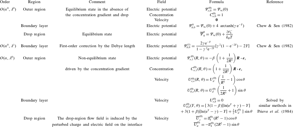
3 Experiments
The diffusiophoresis velocity
 $U_{d}^{(0)}$
is the dimensionless velocity of the drop. Since it is scaled by
$U_{d}^{(0)}$
is the dimensionless velocity of the drop. Since it is scaled by
 $\unicode[STIX]{x1D735}\ln c$
,
$\unicode[STIX]{x1D735}\ln c$
,
 $U_{d}^{(0)}$
can also be deemed as a dimensionless diffusiophoretic mobility (or coefficient), which can further be measured from experiments. To experimentally measure the diffusiophoretic velocity
$U_{d}^{(0)}$
can also be deemed as a dimensionless diffusiophoretic mobility (or coefficient), which can further be measured from experiments. To experimentally measure the diffusiophoretic velocity
 $U_{d}^{(0)}$
of oil droplets with various viscosities, we perform controlled microfluidics experiments using a dead-end geometry where a solute gradient is established along the dead-end channel and induces approximately rectilinear diffusiophoresis of oil droplets. Detailed experimental methods can be found in our previous papers (Shin et al.
Reference Shin, Um, Sabass, Ault, Rahimi, Warren and Stone2016, Reference Shin, Ault, Feng, Warren and Stone2017a
). In brief, the charged droplets in a low NaCl concentration solution are introduced to a dead-end pore containing higher NaCl concentration, leading to diffusiophoresis into the dead-end channel. Upon entry, the droplets form a propagating front because the droplet velocity is proportional to the gradient of the logarithmic solute concentration. The colloidal focusing is a function of the diffusiophoretic mobility, which allows us to extract
$U_{d}^{(0)}$
of oil droplets with various viscosities, we perform controlled microfluidics experiments using a dead-end geometry where a solute gradient is established along the dead-end channel and induces approximately rectilinear diffusiophoresis of oil droplets. Detailed experimental methods can be found in our previous papers (Shin et al.
Reference Shin, Um, Sabass, Ault, Rahimi, Warren and Stone2016, Reference Shin, Ault, Feng, Warren and Stone2017a
). In brief, the charged droplets in a low NaCl concentration solution are introduced to a dead-end pore containing higher NaCl concentration, leading to diffusiophoresis into the dead-end channel. Upon entry, the droplets form a propagating front because the droplet velocity is proportional to the gradient of the logarithmic solute concentration. The colloidal focusing is a function of the diffusiophoretic mobility, which allows us to extract
 $U_{d}^{(0)}$
by visualizing the location of the focused region using a fluorescence microscope (DMI4000B, Leica).
$U_{d}^{(0)}$
by visualizing the location of the focused region using a fluorescence microscope (DMI4000B, Leica).
The oil emulsions with various viscosities are synthesized by a sonication method (Banerjee et al.
Reference Banerjee, Williams, Azevedo, Helgeson and Squires2016). In detail, silicone oil (Sigma-Aldrich, 2 cSt
 ${\leqslant}\overline{\unicode[STIX]{x1D707}}\leqslant$
500 cSt) was initially dyed with an oil-soluble fluorescent dye (TP-3400, Tracer Products) at 0.5 vol. %. Then, 1 vol. % of dyed silicone oil was dispersed in an aqueous solution containing 1 mM sodium dodecyl sulfate (SDS) and 1 mM NaCl by vortex stirring (Analog Vortex Mixer, Fisher Scientific) followed by sonication (Ultrasonic Cleaner, Cole-Parmer) for a certain amount of time depending on the viscosity of the oil. The sizes of the oil droplets were measured using a dynamic light scattering device (Zetasizer Nano-ZS, Malvern), where the average diameter was measured as
${\leqslant}\overline{\unicode[STIX]{x1D707}}\leqslant$
500 cSt) was initially dyed with an oil-soluble fluorescent dye (TP-3400, Tracer Products) at 0.5 vol. %. Then, 1 vol. % of dyed silicone oil was dispersed in an aqueous solution containing 1 mM sodium dodecyl sulfate (SDS) and 1 mM NaCl by vortex stirring (Analog Vortex Mixer, Fisher Scientific) followed by sonication (Ultrasonic Cleaner, Cole-Parmer) for a certain amount of time depending on the viscosity of the oil. The sizes of the oil droplets were measured using a dynamic light scattering device (Zetasizer Nano-ZS, Malvern), where the average diameter was measured as
 ${\approx}0.8~\unicode[STIX]{x03BC}\text{m}$
. To keep the overall SDS concentration constant during the experiment, so as to neglect migration driven by a surface tension gradient, the same concentration of surfactant (1 mM SDS) was added to the initial solution, which has a high concentration of salt (100 mM NaCl). The zeta potential of the droplets was measured using electrophoretic light scattering (Zetasizer Nano-ZS, Malvern Instruments) and a recently developed diffusiophoretic method (Shin et al.
Reference Shin, Ault, Feng, Warren and Stone2017a
), which was measured as
${\approx}0.8~\unicode[STIX]{x03BC}\text{m}$
. To keep the overall SDS concentration constant during the experiment, so as to neglect migration driven by a surface tension gradient, the same concentration of surfactant (1 mM SDS) was added to the initial solution, which has a high concentration of salt (100 mM NaCl). The zeta potential of the droplets was measured using electrophoretic light scattering (Zetasizer Nano-ZS, Malvern Instruments) and a recently developed diffusiophoretic method (Shin et al.
Reference Shin, Ault, Feng, Warren and Stone2017a
), which was measured as
 ${\approx}-87~\text{mV}$
regardless of the droplet viscosity.
${\approx}-87~\text{mV}$
regardless of the droplet viscosity.
The comparison between the analytical result (2.66) and experimental data is shown in figure 3. If
 $\unicode[STIX]{x1D6F7}^{(1)}(0)$
is neglected in (2.66) (the dotted line in figure 3), we find a small deviation from the experimental data. If
$\unicode[STIX]{x1D6F7}^{(1)}(0)$
is neglected in (2.66) (the dotted line in figure 3), we find a small deviation from the experimental data. If
 $\unicode[STIX]{x1D6F7}^{(1)}(0)$
is fitted to be
$\unicode[STIX]{x1D6F7}^{(1)}(0)$
is fitted to be
 $-0.4$
(the solid line in figure 3), then the analytical result and experiments are in good agreement. The moderate value for
$-0.4$
(the solid line in figure 3), then the analytical result and experiments are in good agreement. The moderate value for
 $\unicode[STIX]{x1D6F7}^{(1)}(0)$
also shows that treating it as a fitting parameter is practical.
$\unicode[STIX]{x1D6F7}^{(1)}(0)$
also shows that treating it as a fitting parameter is practical.

Figure 3. The comparison of the analytical results and experiments for the diffusiophoretic velocity as a function of the viscosity ratio
 $\overline{\unicode[STIX]{x1D707}}/\unicode[STIX]{x1D707}$
. The dots and error bars are experimental data. The dotted and solid lines are (2.66), with
$\overline{\unicode[STIX]{x1D707}}/\unicode[STIX]{x1D707}$
. The dots and error bars are experimental data. The dotted and solid lines are (2.66), with
 $\unicode[STIX]{x1D6F7}^{(1)}=0$
and
$\unicode[STIX]{x1D6F7}^{(1)}=0$
and
 $\unicode[STIX]{x1D6F7}^{(1)}=-0.4$
, respectively. The electrolyte solution is NaCl with
$\unicode[STIX]{x1D6F7}^{(1)}=-0.4$
, respectively. The electrolyte solution is NaCl with
 $\unicode[STIX]{x1D6FD}=-0.208$
.
$\unicode[STIX]{x1D6FD}=-0.208$
.
4 Discussion
The diffusiophoretic velocity
 $U_{d}^{(0)}$
of silicone oil drops in NaCl solutions is plotted in figure 4. We observe that the diffusiophoretic speed of a droplet converges to its equivalent solid particle as
$U_{d}^{(0)}$
of silicone oil drops in NaCl solutions is plotted in figure 4. We observe that the diffusiophoretic speed of a droplet converges to its equivalent solid particle as
 $\overline{\unicode[STIX]{x1D707}}/\unicode[STIX]{x1D707}\rightarrow \infty$
. In both figures 3 and 4, we notice that there is a small difference between the droplet and solid-particle velocities because the expression of
$\overline{\unicode[STIX]{x1D707}}/\unicode[STIX]{x1D707}\rightarrow \infty$
. In both figures 3 and 4, we notice that there is a small difference between the droplet and solid-particle velocities because the expression of
 $U_{d,l}^{(0)}$
(2.67b
) contains a prefactor
$U_{d,l}^{(0)}$
(2.67b
) contains a prefactor
 $(1+3\overline{\unicode[STIX]{x1D707}}/\unicode[STIX]{x1D707})^{-1}$
which decreases as the viscosity ratio
$(1+3\overline{\unicode[STIX]{x1D707}}/\unicode[STIX]{x1D707})^{-1}$
which decreases as the viscosity ratio
 $\overline{\unicode[STIX]{x1D707}}/\unicode[STIX]{x1D707}$
increases. The solid-particle result is achieved already by
$\overline{\unicode[STIX]{x1D707}}/\unicode[STIX]{x1D707}$
increases. The solid-particle result is achieved already by
 $\overline{\unicode[STIX]{x1D707}}/\unicode[STIX]{x1D707}\simeq 10$
.
$\overline{\unicode[STIX]{x1D707}}/\unicode[STIX]{x1D707}\simeq 10$
.

Figure 4. The diffusiophoretic velocity in NaCl solutions. The horizontal axis is the dimensionless zeta potential and curves with different viscosity ratios
 $\overline{\unicode[STIX]{x1D707}}/\unicode[STIX]{x1D707}$
are plotted.
$\overline{\unicode[STIX]{x1D707}}/\unicode[STIX]{x1D707}$
are plotted.
 $\unicode[STIX]{x1D6FD}=-0.208$
for NaCl solutions is used and
$\unicode[STIX]{x1D6FD}=-0.208$
for NaCl solutions is used and
 $\unicode[STIX]{x1D6F7}^{(1)}$
is neglected.
$\unicode[STIX]{x1D6F7}^{(1)}$
is neglected.
The velocity fields up to
 $O(\unicode[STIX]{x1D6FC},\unicode[STIX]{x1D706}^{0})$
in the boundary layer (2.48) are the same for drops and solid particles (Prieve et al.
Reference Prieve, Anderson, Ebel and Lowell1984) except for an integration constant
$O(\unicode[STIX]{x1D6FC},\unicode[STIX]{x1D706}^{0})$
in the boundary layer (2.48) are the same for drops and solid particles (Prieve et al.
Reference Prieve, Anderson, Ebel and Lowell1984) except for an integration constant
 $C_{V}$
in (2.48b
). For solid particles
$C_{V}$
in (2.48b
). For solid particles
 $C_{V}$
is determined by the no-slip condition on the interface, while for droplets
$C_{V}$
is determined by the no-slip condition on the interface, while for droplets
 $C_{V}$
is determined by the stress-balance boundary condition (2.57).
$C_{V}$
is determined by the stress-balance boundary condition (2.57).

Figure 5. The velocity field inside the drop and the migration velocity. All the flow fields are sketched in the drop or solid-particle reference frame. The first two figures are the drop-region velocity field (2.56) with (a)
 $\overline{a}_{4}^{(0)}=-1$
and (b)
$\overline{a}_{4}^{(0)}=-1$
and (b)
 $\overline{a}_{4}^{(0)}=1$
and the uniform flow
$\overline{a}_{4}^{(0)}=1$
and the uniform flow
 $U_{d,s}^{(0)}+U_{d,l}^{(0)}$
far away from the drop. (c) The far-field flow velocity
$U_{d,s}^{(0)}+U_{d,l}^{(0)}$
far away from the drop. (c) The far-field flow velocity
 $U_{d,s}^{(0)}$
outside a solid particle. We fix
$U_{d,s}^{(0)}$
outside a solid particle. We fix
 $U_{d,s}^{(0)}>0$
for these three cases (i.e. the uniform flow far away from the solid particle (c) is in the negative
$U_{d,s}^{(0)}>0$
for these three cases (i.e. the uniform flow far away from the solid particle (c) is in the negative
 $x$
direction), then the diffusiophoretic speed of drop (a) is higher than the solid particle (c) because the drop-region flow field is in the same direction as the outer and boundary-layer flow fields. Similarly, the diffusiophoretic speed of drop (b) will be lower than that of (c).
$x$
direction), then the diffusiophoretic speed of drop (a) is higher than the solid particle (c) because the drop-region flow field is in the same direction as the outer and boundary-layer flow fields. Similarly, the diffusiophoretic speed of drop (b) will be lower than that of (c).
A sketch of the drop-region flow field is shown in figure 5. There is only one parameter
 $\overline{a}_{4}^{(0)}$
in the expression of the drop-region flow field (2.56). A change of sign of
$\overline{a}_{4}^{(0)}$
in the expression of the drop-region flow field (2.56). A change of sign of
 $\overline{a}_{4}^{(0)}$
will result in opposite flow directions inside the droplet as shown in figure 5(a,b). To analyse whether this drop-region flow field will increase or decrease the droplet’s diffusiophoretic speed compared with an equivalent solid particle, we first assume the boundary-layer flow is in the positive
$\overline{a}_{4}^{(0)}$
will result in opposite flow directions inside the droplet as shown in figure 5(a,b). To analyse whether this drop-region flow field will increase or decrease the droplet’s diffusiophoretic speed compared with an equivalent solid particle, we first assume the boundary-layer flow is in the positive
 $\unicode[STIX]{x1D703}$
direction (i.e.
$\unicode[STIX]{x1D703}$
direction (i.e.
 $U_{d,s}^{(0)}>0$
) for the solid particle, as shown in figure 5(c). Then, in the laboratory reference frame, this solid particle will move to the left. For a drop, the diffusiophoretic speed will be faster (slower) than its equivalent solid particle if the direction of the drop-region flow field is along the same (opposite) direction of the boundary-layer flow for the solid particle. For example, if
$U_{d,s}^{(0)}>0$
) for the solid particle, as shown in figure 5(c). Then, in the laboratory reference frame, this solid particle will move to the left. For a drop, the diffusiophoretic speed will be faster (slower) than its equivalent solid particle if the direction of the drop-region flow field is along the same (opposite) direction of the boundary-layer flow for the solid particle. For example, if
 $\overline{a}_{4}^{(0)}=-1$
as in figure 5(a), then the drop-region flow is in the same direction as the boundary-layer flow for the solid particle in figure 5(c), which will lead to a higher diffusiophoretic speed for droplets to the left in the laboratory reference frame, and vice versa.
$\overline{a}_{4}^{(0)}=-1$
as in figure 5(a), then the drop-region flow is in the same direction as the boundary-layer flow for the solid particle in figure 5(c), which will lead to a higher diffusiophoretic speed for droplets to the left in the laboratory reference frame, and vice versa.
From (2.62b ), (2.62c ), (2.64a ) and (2.65), we obtain
 $$\begin{eqnarray}\overline{a}_{4}^{(0)}=\frac{1}{2(1+3\overline{\unicode[STIX]{x1D707}}/\unicode[STIX]{x1D707})}(F_{0}^{(2)}\unicode[STIX]{x1D6F7}^{(0)}(0)+F_{0}^{(1)}\unicode[STIX]{x1D6F7}^{(1)}(0)),\end{eqnarray}$$
where
 $F_{0}^{(1)}$
and
$F_{0}^{(1)}$
and
 $F_{0}^{(2)}$
are the charge density at
$F_{0}^{(2)}$
are the charge density at
 $O(\unicode[STIX]{x1D6FC}^{0},\unicode[STIX]{x1D706})$
and
$O(\unicode[STIX]{x1D6FC}^{0},\unicode[STIX]{x1D706})$
and
 $O(\unicode[STIX]{x1D6FC}^{0},\unicode[STIX]{x1D706}^{2})$
on the interface in (2.61) while
$O(\unicode[STIX]{x1D6FC}^{0},\unicode[STIX]{x1D706}^{2})$
on the interface in (2.61) while
 $\unicode[STIX]{x1D6F7}^{(0)}(0)$
and
$\unicode[STIX]{x1D6F7}^{(0)}(0)$
and
 $\unicode[STIX]{x1D6F7}^{(0)}(1)$
are the radial component of the electric potential at
$\unicode[STIX]{x1D6F7}^{(0)}(1)$
are the radial component of the electric potential at
 $O(\unicode[STIX]{x1D6FC},\unicode[STIX]{x1D706}^{0})$
and
$O(\unicode[STIX]{x1D6FC},\unicode[STIX]{x1D706}^{0})$
and
 $O(\unicode[STIX]{x1D6FC}^{0},\unicode[STIX]{x1D706})$
. The appearance of
$O(\unicode[STIX]{x1D6FC}^{0},\unicode[STIX]{x1D706})$
. The appearance of
 $\unicode[STIX]{x1D6F7}(0)$
in (4.1) derives from the tangential electric field in (2.57), i.e.
$\unicode[STIX]{x1D6F7}(0)$
in (4.1) derives from the tangential electric field in (2.57), i.e.
 $$\begin{eqnarray}E_{\unicode[STIX]{x1D703},1}=\frac{1}{R}\frac{\unicode[STIX]{x2202}\unicode[STIX]{x1D6F9}_{1}}{\unicode[STIX]{x2202}\unicode[STIX]{x1D703}}=-\unicode[STIX]{x1D6F7}(0)\sin \unicode[STIX]{x1D703}\quad \text{at }R=1,\end{eqnarray}$$
where
 $E_{\unicode[STIX]{x1D703},1}$
is the tangential electric field at
$E_{\unicode[STIX]{x1D703},1}$
is the tangential electric field at
 $O(\unicode[STIX]{x1D6FC})$
. Also, noticing that the tangential electric field at
$O(\unicode[STIX]{x1D6FC})$
. Also, noticing that the tangential electric field at
 $O(\unicode[STIX]{x1D6FC}^{0})$
is zero because
$O(\unicode[STIX]{x1D6FC}^{0})$
is zero because
 $\unicode[STIX]{x1D6F9}_{0}$
is isotropic, we can conclude that
$\unicode[STIX]{x1D6F9}_{0}$
is isotropic, we can conclude that
 $\overline{a}_{4}^{(0)}$
is the coefficient of the tangential electric stress
$\overline{a}_{4}^{(0)}$
is the coefficient of the tangential electric stress
 $FE_{\unicode[STIX]{x1D703}}$
at
$FE_{\unicode[STIX]{x1D703}}$
at
 $O(\unicode[STIX]{x1D6FC},\unicode[STIX]{x1D706}^{2})$
, though with an opposite sign. This result shows that the drop-region velocity field is driven by the tangential electric stress at the interface, and when
$O(\unicode[STIX]{x1D6FC},\unicode[STIX]{x1D706}^{2})$
, though with an opposite sign. This result shows that the drop-region velocity field is driven by the tangential electric stress at the interface, and when
 $F_{e}E_{\unicode[STIX]{x1D703}}>0$
, the flow direction at the interface is in the positive
$F_{e}E_{\unicode[STIX]{x1D703}}>0$
, the flow direction at the interface is in the positive
 $\unicode[STIX]{x1D703}$
direction (
$\unicode[STIX]{x1D703}$
direction (
 $\overline{a}_{4}^{(0)}<0$
) and vice versa, which also agrees with the features illustrated in figure 5. By comparing (2.65) with (2.67b
), we find that
$\overline{a}_{4}^{(0)}<0$
) and vice versa, which also agrees with the features illustrated in figure 5. By comparing (2.65) with (2.67b
), we find that
 $$\begin{eqnarray}U_{d,l}^{(0)}={\textstyle \frac{2}{3}}\overline{a}_{4}^{(0)},\end{eqnarray}$$
i.e. the term exclusive for drops in the expression of
 $U_{d}^{(0)}$
is just
$U_{d}^{(0)}$
is just
 $\overline{a}_{4}^{(0)}$
with a constant prefactor. In dimensional terms,
$\overline{a}_{4}^{(0)}$
with a constant prefactor. In dimensional terms,
 $$\begin{eqnarray}\boldsymbol{u}_{d,l}^{(0)}=-\frac{2\unicode[STIX]{x1D716}(k_{B}T)^{2}}{3(ze)^{2}(\unicode[STIX]{x1D707}+3\overline{\unicode[STIX]{x1D707}})}\left[6\unicode[STIX]{x1D6FE}(\unicode[STIX]{x1D6FE}+\unicode[STIX]{x1D6FD})+\frac{4\unicode[STIX]{x1D6FE}\unicode[STIX]{x1D6F7}^{(1)}(0)}{1-\unicode[STIX]{x1D6FE}^{2}}\right]\unicode[STIX]{x1D735}\ln c,\end{eqnarray}$$
which we note is independent of size in this leading-order analysis.
The density of the lightest oil droplets used in our experiment is
 $0.91~\text{g}~\text{cm}^{-3}$
. According to Stokes’ law, the density difference can generate a sedimentation velocity of
$0.91~\text{g}~\text{cm}^{-3}$
. According to Stokes’ law, the density difference can generate a sedimentation velocity of
 ${\approx}0.05~\unicode[STIX]{x03BC}\text{m}~\text{s}^{-1}$
, which is much smaller than the typical diffusiophoretic speed
${\approx}0.05~\unicode[STIX]{x03BC}\text{m}~\text{s}^{-1}$
, which is much smaller than the typical diffusiophoretic speed
 ${\approx}1~\unicode[STIX]{x03BC}\text{m}~\text{s}^{-1}$
. In our experiments, gravity is perpendicular to the diffusiophoresis direction. Therefore, the sedimentation should not affect the measurement of diffusiophoretic speeds. In the experiments, the Marangoni effect due to surfactants is singled out by keeping the overall SDS concentration constant. However, the surfactants may ‘rigidify’ the drop surfaces, e.g. in experiments of settling droplets (Edwards, Brenner & Wasan Reference Edwards, Brenner and Wasan1991; Stebe & Maldarelli Reference Stebe and Maldarelli1994). As with other phoretic problems, the shear rate at the surface is
${\approx}1~\unicode[STIX]{x03BC}\text{m}~\text{s}^{-1}$
. In our experiments, gravity is perpendicular to the diffusiophoresis direction. Therefore, the sedimentation should not affect the measurement of diffusiophoretic speeds. In the experiments, the Marangoni effect due to surfactants is singled out by keeping the overall SDS concentration constant. However, the surfactants may ‘rigidify’ the drop surfaces, e.g. in experiments of settling droplets (Edwards, Brenner & Wasan Reference Edwards, Brenner and Wasan1991; Stebe & Maldarelli Reference Stebe and Maldarelli1994). As with other phoretic problems, the shear rate at the surface is
 $O(u/\unicode[STIX]{x1D705}^{-1})$
, which is much larger than the ordinary shear rate
$O(u/\unicode[STIX]{x1D705}^{-1})$
, which is much larger than the ordinary shear rate
 $O(u/a)$
, associated with translational motion (
$O(u/a)$
, associated with translational motion (
 $(\unicode[STIX]{x1D705}a)^{-1}\ll 1$
). Such large shear rates, and corresponding shear stresses, may be why the interface is not ‘rigidified’ by surfactant effects (we thank a referee for this idea).
$(\unicode[STIX]{x1D705}a)^{-1}\ll 1$
). Such large shear rates, and corresponding shear stresses, may be why the interface is not ‘rigidified’ by surfactant effects (we thank a referee for this idea).
Inside the dead-end pore, the salt gradient can also cause a surface tension gradient and result in a Marangoni velocity. The diffusiophoretic speed is proportional to
 $\unicode[STIX]{x1D735}\ln c$
, while the Marangoni velocity is proportional to
$\unicode[STIX]{x1D735}\ln c$
, while the Marangoni velocity is proportional to
 $\unicode[STIX]{x1D735}c$
, and in experiments the Marangoni velocity should be in the opposite direction of diffusiophoresis. As explained in Shin et al. (Reference Shin, Um, Sabass, Ault, Rahimi, Warren and Stone2016), at short times after the oil droplets enter the dead-end pore, the concentration profile along the dead-end pore is approximately an error function. Figure 6 shows the experimental data of velocities for the least viscous oil droplets (
$\unicode[STIX]{x1D735}c$
, and in experiments the Marangoni velocity should be in the opposite direction of diffusiophoresis. As explained in Shin et al. (Reference Shin, Um, Sabass, Ault, Rahimi, Warren and Stone2016), at short times after the oil droplets enter the dead-end pore, the concentration profile along the dead-end pore is approximately an error function. Figure 6 shows the experimental data of velocities for the least viscous oil droplets (
 $\overline{\unicode[STIX]{x1D707}}=1.82~\text{mPa}~\text{s}$
), whose Marangoni effects should be most significant. Using the approaches in Shin et al. (Reference Shin, Um, Sabass, Ault, Rahimi, Warren and Stone2016), we plot the theoretical results of diffusiophoresis (velocity
$\overline{\unicode[STIX]{x1D707}}=1.82~\text{mPa}~\text{s}$
), whose Marangoni effects should be most significant. Using the approaches in Shin et al. (Reference Shin, Um, Sabass, Ault, Rahimi, Warren and Stone2016), we plot the theoretical results of diffusiophoresis (velocity
 $\propto \unicode[STIX]{x1D735}\ln c$
) and Marangoni effects (velocity
$\propto \unicode[STIX]{x1D735}\ln c$
) and Marangoni effects (velocity
 $\propto \unicode[STIX]{x1D735}c$
) and find that the experimental data match with diffusiophoresis theories very well. Therefore, the Marangoni speeds should be at least an order of magnitude slower than the diffusiophoretic speeds. The Marangoni coefficient for silicone oil and water system by adding NaCl is not available in the literature. Based on our analysis, it is predicted to be approximately or less than
$\propto \unicode[STIX]{x1D735}c$
) and find that the experimental data match with diffusiophoresis theories very well. Therefore, the Marangoni speeds should be at least an order of magnitude slower than the diffusiophoretic speeds. The Marangoni coefficient for silicone oil and water system by adding NaCl is not available in the literature. Based on our analysis, it is predicted to be approximately or less than
 $O(10^{-4})~\text{N}~\text{m}^{-1}~\text{M}$
.
$O(10^{-4})~\text{N}~\text{m}^{-1}~\text{M}$
.

Figure 6. Measurement of oil droplet (
 $\overline{\unicode[STIX]{x1D707}}=1.82~\text{mPa}~\text{s}$
) speeds along the dead-end pore at 10 s after entering, compared with theoretical results of diffusiophoresis and Marangoni effects (calculated using approaches outlined in Shin et al. (Reference Shin, Um, Sabass, Ault, Rahimi, Warren and Stone2016)).
$\overline{\unicode[STIX]{x1D707}}=1.82~\text{mPa}~\text{s}$
) speeds along the dead-end pore at 10 s after entering, compared with theoretical results of diffusiophoresis and Marangoni effects (calculated using approaches outlined in Shin et al. (Reference Shin, Um, Sabass, Ault, Rahimi, Warren and Stone2016)).
 $x$
is the entrance distance and
$x$
is the entrance distance and
 $L=400~\unicode[STIX]{x03BC}\text{m}$
is the length of the dead-end pore.
$L=400~\unicode[STIX]{x03BC}\text{m}$
is the length of the dead-end pore.
5 Concluding remarks
In this paper, we use perturbation analysis to solve the concentration, electric and velocity fields for the diffusiophoresis of a charged drop by assuming two small parameters
 $\unicode[STIX]{x1D6FC}$
and
$\unicode[STIX]{x1D6FC}$
and
 $\unicode[STIX]{x1D706}$
, the former representing typical concentration changes at the scale of the drop and the latter the dimensionless double layer thickness. The drop-region flow of the drop will induce an additional term
$\unicode[STIX]{x1D706}$
, the former representing typical concentration changes at the scale of the drop and the latter the dimensionless double layer thickness. The drop-region flow of the drop will induce an additional term
 $U_{d,l}^{(0)}$
(2.67b
) in the expression of the diffusiophoretic speed of a drop
$U_{d,l}^{(0)}$
(2.67b
) in the expression of the diffusiophoretic speed of a drop
 $U_{d}^{(0)}$
(2.66) compared with that of a solid particle
$U_{d}^{(0)}$
(2.66) compared with that of a solid particle
 $U_{d,s}^{(0)}$
(2.67a
). For the diffusiophoresis of a drop, the continuity of velocity at the interface between the drop and solution requires a drop-region flow field and therefore results in a variation of the surface charge density to balance the viscous stress. Whether the diffusiophoretic speed of a drop is faster or slower than its equivalent solid particle depends on the direction of the tangential electric stress at the interface at
$U_{d,s}^{(0)}$
(2.67a
). For the diffusiophoresis of a drop, the continuity of velocity at the interface between the drop and solution requires a drop-region flow field and therefore results in a variation of the surface charge density to balance the viscous stress. Whether the diffusiophoretic speed of a drop is faster or slower than its equivalent solid particle depends on the direction of the tangential electric stress at the interface at
 $O(\unicode[STIX]{x1D6FC},\unicode[STIX]{x1D706}^{2})$
. When the stress is in the same direction as the boundary-layer flow outside the equivalent solid particle (e.g. figure 5), the diffusiophoretic speed of the drop will be faster than its equivalent solid particle and vice versa.
$O(\unicode[STIX]{x1D6FC},\unicode[STIX]{x1D706}^{2})$
. When the stress is in the same direction as the boundary-layer flow outside the equivalent solid particle (e.g. figure 5), the diffusiophoretic speed of the drop will be faster than its equivalent solid particle and vice versa.
Acknowledgements
We thank the Princeton Environmental Institute and the National Science Foundation (CBET-1702693) for support. F.Y. is also grateful for support from Princeton University through the George W. Riesz ’50 *52 SEAS Fellowship. We thank an anonymous referee for pointing out the surface rigidifying effect.
Appendix A
Here we give details to complete the boundary-layer calculation from § 2.7. In order to solve the velocity fields in the boundary layer, we follow Prieve et al. (Reference Prieve, Anderson, Ebel and Lowell1984) and define
 $$\begin{eqnarray}\displaystyle & S(R)={\mathcal{C}}_{+}\text{e}^{\unicode[STIX]{x1D6F9}_{0}-\unicode[STIX]{x1D6F9}_{\infty }(0)}+\unicode[STIX]{x1D6F7}, & \displaystyle\end{eqnarray}$$
 $$\begin{eqnarray}\displaystyle & Q(R)={\mathcal{C}}_{-}\text{e}^{-\unicode[STIX]{x1D6F9}_{0}+\unicode[STIX]{x1D6F9}_{\infty }(0)}-\unicode[STIX]{x1D6F7}. & \displaystyle\end{eqnarray}$$
 $$\begin{eqnarray}\displaystyle & \displaystyle S^{\prime \prime }+\left(\frac{2}{R}-\unicode[STIX]{x1D6F9}_{0}^{\prime }\right)S^{\prime }-\frac{2}{R^{2}}S=(\unicode[STIX]{x1D6FD}-1)Pe_{b}{\mathcal{U}}\unicode[STIX]{x1D6F9}_{0}^{\prime }, & \displaystyle\end{eqnarray}$$
 $$\begin{eqnarray}\displaystyle & \displaystyle Q^{\prime \prime }+\left(\frac{2}{R}+\unicode[STIX]{x1D6F9}_{0}^{\prime }\right)Q^{\prime }-\frac{2}{R^{2}}Q=(\unicode[STIX]{x1D6FD}+1)Pe_{b}{\mathcal{U}}\unicode[STIX]{x1D6F9}_{0}^{\prime }, & \displaystyle\end{eqnarray}$$
 $$\begin{eqnarray}\displaystyle & S=(1-\unicode[STIX]{x1D6FD})R\quad \text{as }R\rightarrow \infty , & \displaystyle\end{eqnarray}$$
 $$\begin{eqnarray}\displaystyle & Q=(1+\unicode[STIX]{x1D6FD})R\quad \text{as }R\rightarrow \infty , & \displaystyle\end{eqnarray}$$
 $$\begin{eqnarray}\displaystyle & S^{\prime }=0\quad \text{at }R=1, & \displaystyle\end{eqnarray}$$
 $$\begin{eqnarray}\displaystyle & Q^{\prime }=0\quad \text{at }R=1. & \displaystyle\end{eqnarray}$$
The outer solution for
 $S$
is
$S$
is
 $S_{o}=AR^{-2}+(1-\unicode[STIX]{x1D6FD})R$
, where
$S_{o}=AR^{-2}+(1-\unicode[STIX]{x1D6FD})R$
, where
 $A$
is a constant (note that in the outer region,
$A$
is a constant (note that in the outer region,
 $\unicode[STIX]{x1D6F9}_{0}^{\prime }=0$
). We expand
$\unicode[STIX]{x1D6F9}_{0}^{\prime }=0$
). We expand
 $A=A^{(0)}+\unicode[STIX]{x1D706}A^{(1)}+\unicode[STIX]{x1D706}^{2}A^{(2)}+\cdots \,$
and substitute
$A=A^{(0)}+\unicode[STIX]{x1D706}A^{(1)}+\unicode[STIX]{x1D706}^{2}A^{(2)}+\cdots \,$
and substitute
 $R=1+\unicode[STIX]{x1D706}Y$
, so that the outer solution becomes
$R=1+\unicode[STIX]{x1D706}Y$
, so that the outer solution becomes
 $$\begin{eqnarray}\displaystyle S_{o} & = & \displaystyle (A^{(0)}+A^{(1)}\unicode[STIX]{x1D706}+A^{(2)}\unicode[STIX]{x1D706}^{2}+\cdots \,)(1+\unicode[STIX]{x1D706}Y)^{-2}+(1-\unicode[STIX]{x1D6FD})(1+\unicode[STIX]{x1D706}Y)\qquad\end{eqnarray}$$
 $$\begin{eqnarray}\displaystyle & = & \displaystyle A^{(0)}+1-\unicode[STIX]{x1D6FD}+A^{(1)}\unicode[STIX]{x1D706}+(1-\unicode[STIX]{x1D6FD}-2A^{(0)})\unicode[STIX]{x1D706}Y+A^{(2)}\unicode[STIX]{x1D706}^{2}-2A^{(1)}\unicode[STIX]{x1D706}^{2}Y+\cdots \,.\qquad\end{eqnarray}$$
 $$\begin{eqnarray}\displaystyle \boldsymbol{e}_{\unicode[STIX]{x1D719}}\boldsymbol{\cdot }\widetilde{\unicode[STIX]{x1D735}}\wedge \widetilde{\unicode[STIX]{x1D6FB}}^{2}U_{1} & = & \displaystyle \frac{\unicode[STIX]{x1D706}^{-2}\sin \unicode[STIX]{x1D703}\unicode[STIX]{x1D6F9}_{0}^{\prime }}{2R}({\mathcal{C}}_{+}-{\mathcal{C}}_{-}+2\cosh [\unicode[STIX]{x1D6F9}_{0}-\unicode[STIX]{x1D6F9}_{\infty }(0)]\unicode[STIX]{x1D6F7})\nonumber\\ \displaystyle & = & \displaystyle \frac{\unicode[STIX]{x1D706}^{-2}\sin \unicode[STIX]{x1D703}\unicode[STIX]{x1D6F9}_{0}^{\prime }}{2R}(S\text{e}^{-\unicode[STIX]{x1D6F9}_{0}+\unicode[STIX]{x1D6F9}_{\infty }}-Q\text{e}^{\unicode[STIX]{x1D6F9}_{0}-\unicode[STIX]{x1D6F9}_{\infty }}).\end{eqnarray}$$
Changing the coordinate variable from
 $R$
to
$R$
to
 $Y$
, the functions (A 1) within the boundary layer are defined as
$Y$
, the functions (A 1) within the boundary layer are defined as
 $$\begin{eqnarray}\displaystyle & S(R)=S(\unicode[STIX]{x1D706}Y+1)=S_{b}(Y), & \displaystyle\end{eqnarray}$$
 $$\begin{eqnarray}\displaystyle & Q(R)=Q(\unicode[STIX]{x1D706}Y+1)=Q_{b}(Y). & \displaystyle\end{eqnarray}$$
 $$\begin{eqnarray}\displaystyle & \displaystyle \unicode[STIX]{x1D706}^{-2}S_{b}^{\prime \prime }+\left(\frac{2}{\unicode[STIX]{x1D706}Y+1}-\unicode[STIX]{x1D706}^{-1}\unicode[STIX]{x1D6F9}_{b,0}^{\prime }\right)\unicode[STIX]{x1D706}^{-1}S_{b}^{\prime }-\frac{2}{(\unicode[STIX]{x1D706}Y+1)^{2}}S_{b}=(\unicode[STIX]{x1D6FD}-1)Pe_{b}{\mathcal{U}}_{b}\unicode[STIX]{x1D706}^{-1}\unicode[STIX]{x1D6F9}_{b,0}^{\prime },\quad & \displaystyle\end{eqnarray}$$
 $$\begin{eqnarray}\displaystyle & \displaystyle \unicode[STIX]{x1D706}^{-2}Q_{b}^{\prime \prime }+\left(\frac{2}{\unicode[STIX]{x1D706}Y+1}+\unicode[STIX]{x1D706}^{-1}\unicode[STIX]{x1D6F9}_{b,0}^{\prime }\right)\unicode[STIX]{x1D706}^{-1}Q_{b}^{\prime }-\frac{2}{(\unicode[STIX]{x1D706}Y+1)^{2}}Q_{b}=(\unicode[STIX]{x1D6FD}+1)Pe_{b}{\mathcal{U}}_{b}\unicode[STIX]{x1D706}^{-1}\unicode[STIX]{x1D6F9}_{b,0}^{\prime }.\qquad & \displaystyle\end{eqnarray}$$
 $$\begin{eqnarray}\displaystyle & & \displaystyle \unicode[STIX]{x1D706}^{-3}{\mathcal{V}}_{b}^{\prime \prime \prime }\sin \unicode[STIX]{x1D703}-\frac{2{\mathcal{V}}_{b}^{\prime }\cos \unicode[STIX]{x1D703}}{\unicode[STIX]{x1D706}(\unicode[STIX]{x1D706}Y+1)^{2}\sin \unicode[STIX]{x1D703}}+\frac{3{\mathcal{V}}_{b}^{\prime \prime }\sin \unicode[STIX]{x1D703}}{\unicode[STIX]{x1D706}^{2}(\unicode[STIX]{x1D706}Y+1)}+\frac{2{\mathcal{V}}_{b}\cos \unicode[STIX]{x1D703}}{(\unicode[STIX]{x1D706}Y+1)^{3}\sin \unicode[STIX]{x1D703}}+\frac{2{\mathcal{U}}_{b}\cos \unicode[STIX]{x1D703}}{(\unicode[STIX]{x1D706}Y+1)^{3}}\nonumber\\ \displaystyle & & \displaystyle \quad +\,\frac{{\mathcal{U}}_{b}^{\prime \prime }\sin \unicode[STIX]{x1D703}}{\unicode[STIX]{x1D706}^{2}(\unicode[STIX]{x1D706}Y+1)}=\frac{\unicode[STIX]{x1D6F9}_{b,0}^{\prime }\sin \unicode[STIX]{x1D703}}{2\unicode[STIX]{x1D706}^{3}(\unicode[STIX]{x1D706}Y+1)}(S_{b}\text{e}^{-\unicode[STIX]{x1D6F9}_{b,0}+\unicode[STIX]{x1D6F9}_{\infty }(0)}-Q_{b}\text{e}^{\unicode[STIX]{x1D6F9}_{b,0}-\unicode[STIX]{x1D6F9}_{\infty }(0)}).\end{eqnarray}$$
The expansions (in terms of
 $\unicode[STIX]{x1D706}$
) of (A 7a
) are
$\unicode[STIX]{x1D706}$
) of (A 7a
) are
 $$\begin{eqnarray}(S_{b}^{(0)})^{\prime \prime }-(\unicode[STIX]{x1D6F9}_{b,0}^{(0)})^{\prime }(S_{b}^{(0)})^{\prime }=0,\end{eqnarray}$$
 $$\begin{eqnarray}(S_{b}^{(1)})^{\prime \prime }+2(S_{b}^{(0)})^{\prime }-(\unicode[STIX]{x1D6F9}_{b,0}^{(1)})^{\prime }(S_{b}^{(0)})^{\prime }-(\unicode[STIX]{x1D6F9}_{b,0}^{(0)})^{\prime }(S_{b}^{(1)})^{\prime }=(\unicode[STIX]{x1D6FD}-1)Pe_{b}{\mathcal{U}}_{b}^{(0)}(\unicode[STIX]{x1D6F9}_{b,0}^{(0)})^{\prime },\end{eqnarray}$$
 $$\begin{eqnarray}\displaystyle & & \displaystyle (S_{b}^{(2)})^{\prime \prime }+2(S_{b}^{(1)})^{\prime }-2Y(S_{b}^{(0)})^{\prime }-(\unicode[STIX]{x1D6F9}_{b,0}^{(2)})^{\prime }(S_{b}^{(0)})^{\prime }-(\unicode[STIX]{x1D6F9}_{b,0}^{(1)})^{\prime }(S_{b}^{(1)})^{\prime }\nonumber\\ \displaystyle & & \displaystyle \quad -\,(\unicode[STIX]{x1D6F9}_{b,0}^{(0)})^{\prime }(S_{b}^{(2)})^{\prime \prime }-2S_{b}^{(0)}=(\unicode[STIX]{x1D6FD}-1)Pe_{b}[{\mathcal{U}}_{b}^{(0)}(\unicode[STIX]{x1D6F9}_{b,0}^{(1)})^{\prime }+{\mathcal{U}}_{b}^{(1)}(\unicode[STIX]{x1D6F9}_{b,0}^{(0)})^{\prime }].\end{eqnarray}$$
Solving (A 9a ) with the boundary condition (A 3c ) gives
 $$\begin{eqnarray}(S_{b}^{(0)})^{\prime }=0.\end{eqnarray}$$
By matching with the outer solution (A 4b ), we have
 $$\begin{eqnarray}S_{b}^{(0)}=A^{(0)}+1-\unicode[STIX]{x1D6FD}.\end{eqnarray}$$
Using (A 11) and
 ${\mathcal{U}}_{b}^{(0)}=0$
from (2.48a
), we can deduce that
${\mathcal{U}}_{b}^{(0)}=0$
from (2.48a
), we can deduce that
 $S_{b}^{(1)}$
is also a constant. By matching
$S_{b}^{(1)}$
is also a constant. By matching
 $O(\unicode[STIX]{x1D706}^{1})$
and
$O(\unicode[STIX]{x1D706}^{1})$
and
 $O(\unicode[STIX]{x1D706}Y)$
in (A 4b
), we have
$O(\unicode[STIX]{x1D706}Y)$
in (A 4b
), we have
 $$\begin{eqnarray}\displaystyle & S_{b}^{(1)}=A^{(1)}, & \displaystyle\end{eqnarray}$$
 $$\begin{eqnarray}\displaystyle & 1-\unicode[STIX]{x1D6FD}-2A^{(0)}=0. & \displaystyle\end{eqnarray}$$
 $$\begin{eqnarray}S_{b}^{(0)}=\frac{3(1-\unicode[STIX]{x1D6FD})}{2}.\end{eqnarray}$$
Equation (A 9c ) then becomes
 $$\begin{eqnarray}(S_{b}^{(2)})^{\prime \prime }-(\unicode[STIX]{x1D6F9}_{b,0}^{(0)})^{\prime }(S_{b}^{(2)})^{\prime }=2S_{b}^{(0)}-[2+(\unicode[STIX]{x1D6F9}_{b,0}^{(1)})^{\prime }](S_{b}^{(1)})^{\prime }+(\unicode[STIX]{x1D6FD}-1)Pe_{b}U_{1}(\unicode[STIX]{x1D6F9}_{b,0}^{(0)})^{\prime }\end{eqnarray}$$
and the solution is
 $$\begin{eqnarray}(S_{b}^{(2)})^{\prime }=\text{e}^{\unicode[STIX]{x1D6F9}_{b,0}^{(0)}-\unicode[STIX]{x1D6F9}_{\infty }(0)}\int _{0}^{Y}\text{e}^{-\unicode[STIX]{x1D6F9}_{b,0}^{(0)}+\unicode[STIX]{x1D6F9}_{\infty }(0)}[2S_{b}^{(0)}+(\unicode[STIX]{x1D6FD}-1)Pe_{b}{\mathcal{U}}_{b}^{(1)}(\unicode[STIX]{x1D6F9}_{b,0}^{(0)})^{\prime }]\,\text{d}s+C_{s}\text{e}^{\unicode[STIX]{x1D6F9}_{b,0}^{(0)}-\unicode[STIX]{x1D6F9}_{\infty }(0)},\end{eqnarray}$$
where
 $C_{s}$
is an integration constant. The boundary condition (A 3c
) determines
$C_{s}$
is an integration constant. The boundary condition (A 3c
) determines
 $C_{s}=0$
. Next, matching with the
$C_{s}=0$
. Next, matching with the
 $O(\unicode[STIX]{x1D706}^{2}Y)$
term in (A 4b
), we have
$O(\unicode[STIX]{x1D706}^{2}Y)$
term in (A 4b
), we have
 $$\begin{eqnarray}S_{b}^{(1)}=A^{(1)}=-\frac{1-\unicode[STIX]{x1D6FD}}{2}\left[3\int _{0}^{\infty }(\text{e}^{-\unicode[STIX]{x1D6F9}_{b,0}^{(0)}+\unicode[STIX]{x1D6F9}_{\infty }(0)}-1)\,\text{d}Y-Pe_{b}\int _{0}^{\infty }{\mathcal{U}}_{b}^{(1)}\text{e}^{-\unicode[STIX]{x1D6F9}_{b,0}^{(0)}+\unicode[STIX]{x1D6F9}_{\infty }(0)}(\unicode[STIX]{x1D6F9}_{b,0}^{(0)})^{\prime }\,\text{d}Y\right].\end{eqnarray}$$
Similarly, we can solve for the
 $O(\unicode[STIX]{x1D706}^{0})$
and
$O(\unicode[STIX]{x1D706}^{0})$
and
 $O(\unicode[STIX]{x1D706}^{1})$
of
$O(\unicode[STIX]{x1D706}^{1})$
of
 $Q_{b}$
, i.e.
$Q_{b}$
, i.e.
 $$\begin{eqnarray}\displaystyle & \displaystyle Q_{b}^{(0)}=\frac{3(1+\unicode[STIX]{x1D6FD})}{2}, & \displaystyle\end{eqnarray}$$
 $$\begin{eqnarray}\displaystyle & \displaystyle Q_{b}^{(1)}=-\frac{1+\unicode[STIX]{x1D6FD}}{2}\left[3\int _{0}^{\infty }(\text{e}^{\unicode[STIX]{x1D6F9}_{b,0}^{(0)}-\unicode[STIX]{x1D6F9}_{\infty }}-1)\,\text{d}Y+Pe_{b}\int _{0}^{\infty }{\mathcal{U}}_{b}^{(1)}\text{e}^{\unicode[STIX]{x1D6F9}_{b,0}^{(0)}-\unicode[STIX]{x1D6F9}_{\infty }}(\unicode[STIX]{x1D6F9}_{0}^{(0)})^{\prime }\,\text{d}Y\right].\qquad & \displaystyle\end{eqnarray}$$
The
 $O(\unicode[STIX]{x1D706}^{0})$
terms in equation (A 8) are
$O(\unicode[STIX]{x1D706}^{0})$
terms in equation (A 8) are
 $$\begin{eqnarray}({\mathcal{V}}_{b}^{(0)})^{\prime \prime \prime }=\frac{(\unicode[STIX]{x1D6F9}_{b,0}^{(0)})^{\prime }}{2}(S_{b}^{(0)}\text{e}^{-\unicode[STIX]{x1D6F9}_{b,0}^{(0)}+\unicode[STIX]{x1D6F9}_{\infty }}-Q_{b}^{(0)}\text{e}^{\unicode[STIX]{x1D6F9}_{b,0}^{(0)}-\unicode[STIX]{x1D6F9}_{\infty }}).\end{eqnarray}$$
Integrating (A 18) leads to
 $$\begin{eqnarray}({\mathcal{V}}_{b}^{(0)})^{\prime }=-\frac{2S_{b}^{(0)}\unicode[STIX]{x1D6FE}}{\text{e}^{Y}+\unicode[STIX]{x1D6FE}}+\frac{2Q_{b}^{(0)}\unicode[STIX]{x1D6FE}}{\text{e}^{Y}-\unicode[STIX]{x1D6FE}},\end{eqnarray}$$
from which we find
 $$\begin{eqnarray}{\mathcal{V}}_{b}^{(0)}=2S_{b}^{(0)}[\ln (\text{e}^{Y}+\unicode[STIX]{x1D6FE})-Y]+2Q_{b}^{(0)}[\ln (\text{e}^{Y}-\unicode[STIX]{x1D6FE})-Y]+C_{V},\end{eqnarray}$$
where
 $C_{V}$
is a constant. The continuity equation within the boundary layer yields
$C_{V}$
is a constant. The continuity equation within the boundary layer yields
 $$\begin{eqnarray}\displaystyle & ({\mathcal{U}}_{b}^{(0)})^{\prime }=0, & \displaystyle\end{eqnarray}$$
 $$\begin{eqnarray}\displaystyle & ({\mathcal{U}}_{b}^{(1)})^{\prime }=-2{\mathcal{V}}_{b}^{(0)}. & \displaystyle\end{eqnarray}$$
 ${\mathcal{U}}_{b}^{(0)}(Y)$
is constant. In order to satisfy
${\mathcal{U}}_{b}^{(0)}(Y)$
is constant. In order to satisfy
 ${\mathcal{U}}_{b}(Y=0)=0$
, we have
${\mathcal{U}}_{b}(Y=0)=0$
, we have  $$\begin{eqnarray}{\mathcal{U}}_{b}^{(0)}(Y)=0.\end{eqnarray}$$


