


1. Introduction
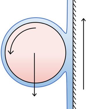
A vertical wall is covered in a thin layer of oil that is sufficiently viscous for drainage effects to be negligible. When a cylinder is placed on the wall with its axis horizontal, it will roll down the wall. However, if the wall is translated upwards, is it possible to keep the centre of the cylinder fixed in place in the laboratory frame by adjusting the speed of the wall? In this paper, we will address this question, which is an example of steady levitation by a viscous fluid.
Levitation of solids and liquids by acoustic or magnetic forces is a well-studied area, but levitation by hydrodynamic forces has received less attention. Thin-film levitation has been studied by, for example, Hinch & Lemaitre (Reference Hinch and Lemaitre1994), Fitt, Kozyreff & Ockendon (Reference Fitt, Kozyreff and Ockendon2004), de Maleprade et al. (Reference de Maleprade, Soto, Quéré, Hinch, Baier, Schür and Hardt2018), Lhuissier et al. (Reference Lhuissier, Tagawa, Tran and Sun2013), and Sawaguchi et al. (Reference Sawaguchi, Matsuda, Hama, Saito and Tagawa2019). All these studies investigate different configurations to the one considered here. Our work builds on the studies of levitation by vertical belts initiated by Eggers, Kerswell & Mullin (Reference Eggers, Kerswell and Mullin2013) for a cylinder and by Mullin, Ockendon & Ockendon (Reference Mullin, Ockendon and Ockendon2020) for a block. Although our work has been driven by scientific curiosity, we will find that it has relevance to practical problems such as the lubrication of bearings and coating flows.
We carry out a theoretical and experimental investigation of a rigid circular cylinder placed horizontally on a vertical belt moving upwards and covered by a thin layer of oil. A schematic of the experiment is shown in figure 1. We are interested in the case in which the cylinder centre remains at a fixed position in the laboratory frame with an appropriate choice of the belt speed. As the belt moves upwards, the cylinder rotates about its own axis at a rate that is lower than the associated slip velocity induced by the belt. Rotation also occurs in the problem of a sphere travelling down an inclined plane covered with a thin viscous film, which was investigated in Bico et al. (Reference Bico, Ashmore-Chakrabarty, McKinley and Stone2009). The geometry of our experiment is similar to those in coating flows, see, for example, Ruschak (Reference Ruschak1985), Duffy & Wilson (Reference Duffy and Wilson1999) and Weinstein & Ruschak (Reference Weinstein and Ruschak2004), and this experiment is also related to the film-splitting flow described by Coyle, Macosko & Scriven (Reference Coyle, Macosko and Scriven1986).

Figure 1. Schematic diagram of the experimental apparatus showing a cylinder balanced on the belt, which is covered in a layer of oil. Videos of this experiment are provided as supplementary material (Movies 1 and 2) available at https://doi.org/10.1017/jfm.2021.284.
The experimental set-up we consider has been modelled previously by Eggers et al. (Reference Eggers, Kerswell and Mullin2013) within a lubrication framework. While successful in determining the qualitative relationship between cylinder rotation rate and belt speed required for levitation, their model did not account for the flow travelling around the cylinder, nor the coalescence/separation flow regions at the inlet/outlet to the lubrication region, and their theoretical results did not agree quantitatively with the experimental data presented therein. This motivates a more comprehensive approach detailed in the present work, in which we specifically account for the fluid travelling around the cylinder and investigate the important inner problem for the full system. These differences lead to different solutions from those in Eggers et al. (Reference Eggers, Kerswell and Mullin2013), and mean that we are able to formally close the complex mathematical system. Our solutions show good agreement with the experimental data. Moreover, we are able to shed light on the onset of fluid tongues in the experiment.
There are several crucial distinctions between levitating a cylinder, which we investigate here, and levitating a block, which was considered in Mullin et al. (Reference Mullin, Ockendon and Ockendon2020). Most obviously, with a cylinder, the downstream fluid forms a coating flow around the top of the cylinder, and rejoins with the fluid upstream of the cylinder, as shown in figure 1. With a block, the fluid passes between the block and the belt, and the top side of the block remains dry. Additionally, the cylinder rotates about its own axis while a block does not. Moreover, in the case of a cylinder, it is observed that there is a unique belt speed that levitates the cylinder. This is different to the case of a block levitating on a thin viscous film, where a continuum of belt speeds resulting in levitation is possible for a given block. In addition, a block has two degrees of freedom in its position – the height of its midpoint from the belt, and the angle it makes with the belt. The cylinder loses a degree of freedom related to an angle, but gains a degree of freedom in its rotation rate. Moreover, the position of the air–oil free surface relative to the lubrication region underneath the block is known a priori – it is located at the ends of the block. However, this is not the case with a cylinder. The positions of the inlet and outlet terminating menisci must be determined as part of the solution, adding two additional degrees of freedom to the system.
In the block levitation considered in Mullin et al. (Reference Mullin, Ockendon and Ockendon2020), there was usually a fluid tongue that propagated downwards at a uniform speed from the corner of the block. This meant there was no steady state in the system and so the fluid flux leaving the system downstream of the block was not equal to the flux entering the system far upstream of the tongue. The presence of a tongue is fundamental to the ability of a block to levitate on a moving belt. The action of the tongue is different in the case of a cylinder, where one of two types of tongue behaviour is possible; both are shown in figure 2. In the first type, the tongue is very small and does not grow with time. The experimental data in Eggers et al. (Reference Eggers, Kerswell and Mullin2013) is all of the first type. In the second type, there is a much longer tongue, which grows with a velocity approximately 20–100 times slower than the belt speed, and the tongue either reaches a fixed length or reaches the bottom of the belt. Tongues do not form for cylinders with larger radii, but as the cylinder radius is decreased there is a critical radius at which a tongue starts to form. After this point, a small decrease in cylinder radius results in a much longer tongue at steady state.

Figure 2. Tongues arising from cylinder levitation on  $0.3$ mm layers of silicone oil. (a) A 12 mm long, 5 mm diameter PTFE cylinder, exhibiting a short tongue. (b) A 12 mm long, 4 mm diameter PTFE cylinder, exhibiting a long tongue. (c) A 15 mm long, 8 mm diameter hollow aluminium cylinder, exhibiting an incipient tongue.
In this paper, we present a steady two-dimensional model for the coupled fluid flow and cylinder motion problem. We analyse this model using a combination of the method of matched asymptotic expansions and direct numerical simulation (DNS), and compare its predictions with the experimental results. While our asymptotic analysis reveals that the majority of the important behaviour occurs within the lubrication region between the belt and cylinder, this region has an a priori unknown finite extent. Hence, the endpoints of the lubrication region must be determined as part of the solution, resulting in a free-boundary problem. To close the asymptotically reduced system, we must solve a non-trivial inner problem near the upper meniscus, which we derive systematically. To solve for the flow in this region, we use a powerful (but expensive) numerical approach, allowing us to efficiently target the use of computational resources to the region that closes the problem. Our strategy ensures we can characterise the flow over a wide range of parameters, while successfully validating our model by comparison to the available experimental data.
The structure of this paper is as follows. We first describe the experiment in § 2. We present a dimensional description of a model that neglects gravitational forces in the liquid in § 3, which we subsequently non-dimensionalise. We solve this system in § 4, using a combination of asymptotic and numerical techniques, and validate our results against the experimental data. In § 5, we briefly assess the importance of gravitational forces in the liquid and the possible occurrence of tongues, before discussing our results and some open questions in § 6.
2. Experimental set-up
A 375 mm long and 26.5 mm wide steel-reinforced plastic timing belt was driven vertically, as shown in the schematic diagram of the apparatus in figure 1. The outside of the belt provided a smooth moving surface of length 150 mm. The belt was driven by one of a pair of 38 mm toothed pulleys which were matched to the teeth on the inside of the belt. The drive was provided by a DC motor with a controlled feedback loop which was connected to the drive pulley through a 50 : 1 gearbox. The rotation rate of the drive was measured using a calibrated optical shaft encoder.
The viscous fluid was silicone oil with a measured dynamic viscosity of  $\tilde {\mu } = 13\,341\pm 50$ cP at
  $21\,^{\circ }\textrm {C}$. The experiments were carried out in a controlled environment where the temperature of the oil was measured to be
  $21 \pm 0.5\,^{\circ }\textrm {C}$. The density of the silicone oil was
  $\tilde {\rho } = 0.971\pm 0.001\ \textrm {g}\ \textrm {cm}^{-3}$ and the oil–air surface tension was
  $\tilde {\gamma } = 21.5\ \textrm {mN}\ \textrm {m}^{-1}$. Silicone oil readily coats and wets the belt, which enabled the formation of a uniform layer. The belt passed through a 2 cm deep bath of oil and the thickness of the layer was set using a knife edge which acted as a scraper fixed at a controlled distance from the belt, which was set between 0.1–1 mm. The uniformity and depth of the layer were measured using a commercial confocal optical device from Micro-Epsilon (confocalDT). It was found to be constant to within
  $10\,\%$ over the central portion of the belt.
The cylinders were made from polytetrafluoroethylene (PTFE), also known as Teflon®, and had a density of  $\tilde {\rho }_s = 2.2\ \textrm {g}\ \textrm {cm}^{-3}$. The cylinder length was always 12 mm, and the cylinder radius ranged from
  $\tilde {a} = 2\text {--}8\ \textrm {mm}$. The belt speed required to levitate these cylinders ranged between
  $\tilde {U}_b = 1\text {--}35\ \textrm {mm}\ \textrm {s}^{-1}$. A few experiments on tongue development were performed using plastic printed cylinders. These cylinders had lengths of 12.35 mm, diameters of 5.80–7.95 mm, and were printed using the material acrylonitrile butadiene styrene (ABS), which has a density of
  $1.04\ \textrm {g}\ \textrm {cm}^{-3}$.
2.1. Experimental protocols
The apparatus was run for an initial period of 30 min to establish a uniform film of viscous fluid on the belt before any levitation experiment was carried out. The thickness of the film was set using the knife edge. Achieving levitation with cylinders was relatively straightforward and involved placing a cylinder on the moving layer and adjusting the speed of the belt to achieve balance. If the belt speed was too high, the cylinder moved up the belt, too low and it travelled down the belt. A given cylinder would always rotate around its own axis at a rate that was found to be independent of the belt speed. A typical set of results illustrating these points are shown in figure 3. It can be seen in figure 3(a) that there is a linear relationship between the belt speed and the cylinder translation velocity, and that the translation speed is zero for a particular belt speed, i.e. the cylinder is balanced at a unique belt speed. The gradient of this linear relationship is approximately  $1$. This is because the problem of determining the belt speed required for levitation is equivalent to determining the cylinder fall speed with a stationary belt for the following reason. The cylinder translates at an approximately uniform speed, since inertial terms are small, and so the frame moving with the cylinder is inertial. At this specific belt speed, the cylinder centre is stationary in the laboratory frame while the cylinder continues to rotate about its own axis. This balance was observed to be stable over a time scale of at least 12 h. Note that the balance speed and cylinder rotation rate were dependent on the size and weight of cylinder used. Occasionally, a mild rippling in the free surface is observed downstream of the cylinder, analogous to the classic printer's instability (Pearson Reference Pearson1960), but this does not appear to affect the cylinder motion.

Figure 3. (a) The translation velocity of a cylinder in the laboratory frame. The dashed black line represents a cylinder that is fixed in the laboratory frame, so below/above this line the cylinder moves down/up the belt. The solid blue line shows a linear best fit of the data. (b) The rotation velocity (rotation rate multiplied by cylinder radius) of the same cylinder, which we see is essentially independent of belt speed. For these data, we use an 8 mm diameter, 12 mm long PTFE cylinder on a 0.3 mm oil layer. The data are collected by measuring the time taken for the cylinder to translate 100 mm, and averaged over 10 repetitions. The error bars correspond to one standard deviation of the data.
The majority of the experiments were performed with cylinders with radii which were larger than the layer thickness by a factor of approximately  $10$. In these cases, a small stable tongue was observed to form on the upstream side of the cylinder as in figure 2(a). For smaller cylinders, the tongue could grow to much longer lengths, as shown in figure 2(b). Part of our modelling work will involve understanding the onset of tongue formation. We will consider a two-dimensional model of the fluid problem, neglecting any edge effects near the ends of the cylinder (e.g. deformations in the fluid surface near the ends of the cylinder in figure 2). Even with these assumptions, the model predicts results that agree well with experimental data.
3. Mathematical model
We model the steady state of the experiment described in § 2. We consider the motion of a rigid circular cylinder which sits on a thin layer of oil covering a moving wall. We consider a two-dimensional cross-section of the cylinder, with coordinate system  $(\tilde {x},\tilde {y})$ centred on the belt at the closest point to the cylinder, i.e. the nip point, aligned such that the positive
  $\tilde {x}$-axis is in the direction of the moving belt and the positive
  $\tilde {y}$-axis points from belt to cylinder. We use tildes to denote dimensional quantities throughout. We will model the flow of the viscous fluid and the position of its free surface, and couple this to the motion of the cylinder, each of which must be determined as part of the solution. The fluid velocity is denoted as
  $\tilde {\boldsymbol {u}} = \tilde {u} \boldsymbol {e}_{\tilde {x}} + \tilde {v} \boldsymbol {e}_{\tilde {y}}$, where
  $\boldsymbol {e}_{\tilde {x}}$ and
  $\boldsymbol {e}_{\tilde {y}}$ are the unit vectors in the
  $\tilde {x}$ and
  $\tilde {y}$-directions, respectively, and the fluid pressure is denoted as
  $\tilde {p}$. We provide a schematic of the model set-up in figure 4.

Figure 4. Schematic of the model we consider in this paper. The lower (hashed) black line denotes the belt, the circle denotes the cylinder, and the blue line denotes the fluid free surface. For lighter cylinders, a tongue may form on the upstream side of the cylinder.
Since the Reynolds number based on a typical cylinder radius and belt speed is of  $\mathit {O}(10^{-3})$, the dimensional governing equations within the fluid are the incompressible steady Stokes flow equations:
 \begin{equation} \tilde{\boldsymbol{\nabla}} \tilde{p} = \tilde{\mu} \tilde{\nabla}^2 \tilde{\boldsymbol{u}} - \tilde{\rho} \tilde{g} \boldsymbol{e}_{\tilde{x}}, \quad \tilde{\boldsymbol{\nabla}} \boldsymbol{\cdot} \tilde{\boldsymbol{u}} = 0, \end{equation}
where the (constant) parameters are the fluid dynamic viscosity  $\tilde {\mu }$, the fluid density
  $\tilde {\rho }$ and the acceleration due to gravity
  $\tilde {g}$.
At the solid boundaries, the fluid satisfies the no-slip condition. Therefore, on the belt, we impose the boundary condition
 \begin{equation} \tilde{\boldsymbol{u}} = \tilde{U}_b \boldsymbol{e}_{\tilde{x}}, \end{equation}
where  $\tilde {U}_b$ is the a priori unknown belt velocity, and on the cylinder surface we impose
 \begin{equation} \tilde{\boldsymbol{u}} = \tilde{a} \tilde{\varOmega} \boldsymbol{t}, \end{equation}
where  $\tilde {a}$ is the cylinder radius and
  $\tilde {\varOmega }$ is the a priori unknown angular velocity of the cylinder. Here,
  $\boldsymbol {t}$ is the unit vector tangent to the cylinder surface in the anticlockwise direction.
At the free fluid–air boundary, the normal stress is balanced by surface tension, and the tangential stress vanishes, yielding
 \begin{equation} \boldsymbol{\tilde{\sigma}} \boldsymbol{\cdot} \boldsymbol{n} = \tilde{\gamma} \left(\tilde{\nabla} \boldsymbol{\cdot} \boldsymbol{n} \right) \boldsymbol{n}, \end{equation}
where  $\boldsymbol{\tilde{\sigma}}$ is the stress tensor of the fluid,
  $\tilde {\gamma }$ is the (constant) fluid–air surface tension and
  $\boldsymbol {n}$ points out of the fluid.
Far upstream, the film thickness is prescribed and the free surface, described by  $\tilde {y} = \tilde {H}(\tilde {x})$, satisfies
 \begin{equation} \tilde{H} \to \tilde{h} \quad \text{as } \tilde{x} \to -\infty, \end{equation}
where  $\tilde {h}$ is the imposed upstream film thickness. Far downstream, the film thickness is uniform and the free surface satisfies
 \begin{equation} \frac{\mathrm{d} \tilde{H}}{\mathrm{d} \tilde{x}} \to 0 \quad \text{as } \tilde{x} \to \infty. \end{equation}
The force and torque acting on the cylinder result from gravity and the fluid stress. Since we are considering a cylinder whose centre is fixed in the laboratory frame, the dimensional force balance is
 \begin{equation} {\rm \pi}\tilde{a}^2 \tilde{\rho}_s \tilde{g} \boldsymbol{e}_{\tilde{x}} = \oint_{\partial \tilde{S}} \boldsymbol{\tilde{\sigma}} \boldsymbol{\cdot} \boldsymbol{n} \, \mathrm{d}\tilde{S}, \end{equation}
where  ${\rm \pi} \tilde {a}^2 \tilde {\rho }_s$ is the mass of the cylinder per unit length,
  $\tilde {\rho }_s$ is the cylinder density, and
  $\partial \tilde {S}$ is the surface of the two-dimensional cross-section of the cylinder. In a similar manner, the dimensional torque balance yields
 \begin{equation} \oint_{\partial \tilde{S}} \tilde{\boldsymbol{r}} \times \left(\boldsymbol{\tilde{\sigma}} \boldsymbol{\cdot} \boldsymbol{n}\right) \mathrm{d}\tilde{S} = \boldsymbol{0}, \end{equation}
where  $\tilde {\boldsymbol {r}}$ is the position vector of a point on the surface of the cylinder with respect to the centre of the cylinder.
The experimental parameter values are given in § 2, and summarised for convenience in table 1. At this point, we emphasise that the belt speed  $\tilde {U}_b$ and the cylinder rotation rate
  $\tilde {\varOmega }$ are initially unknown for a given cylinder, and must be determined as a function of the remaining system parameters. Moreover, of the various parameters to be calculated as part of the solution,
  $\tilde {U}_b$ and
  $\tilde {\varOmega }$ are the most easily measurable experimental quantities; they will serve as helpful quantities with which to validate our model.
Table 1. The experimental parameters referred to in § 2, the parameters to which we refer in our mathematical model, and the typical values of each.

3.1. Asymptotic structure
Since the ratio  $\tilde {h}/\tilde {a} =: \epsilon$ is small, we expect to be able to model much of the flow by lubrication theory. However, before we non-dimensionalise the system, it is helpful to understand the asymptotic regions present in the flow problem in the limit
  $\epsilon \to 0$, in order to focus on the most important regions. As such, we now outline the asymptotic structure of the dimensionless problem with lengths scaled with cylinder radius.
In the limit  $\epsilon \to 0$, there are six asymptotic regions in the system, as illustrated in figure 5. The first region (Region I) is the thin layer of oil between the scraper at the bottom of the belt and the tip of any tongue created by the cylinder. Scaling length with cylinder radius, it has thickness
  $\epsilon$ and length of
  $\mathit {O}(1)$. In this region, the fluid from the scraper is undisturbed – the fluid moves up the belt with a free surface parallel to the belt.

Figure 5. A schematic of the asymptotic regions involved in the dimensionless system, assuming no tongue formation. The regions with boundaries denoted as dashed green lines are lubrication regions and those denoted with dotted red lines are transition regions. All lengths are measured relative to the cylinder radius.
Region II is the small upstream coalescence region representing the inlet of the nip region between the belt and the cylinder. The flow is two-dimensional here and so, in the absence of a tongue, its thickness and length are of  $\mathit {O}(\epsilon )$. In Region II, the cylinder is physically present in the problem, but its surface appears flat here (not shown in figure 5). This is in contrast to the free surface, whose curvature is apparent at leading order in this region. This inlet region marks the three-way transition between the fluid coming in from over the cylinder (Region VI, discussed below), the fluid entering from upstream (Region I), and the fluid entering the nip region between the belt and the cylinder (Region III, discussed below). The extent of Region II must be determined as part of the solution.
Region III is the thin nip region between the belt and the cylinder. Its thickness is of  $\mathit {O}(\epsilon )$ and, since the cylinder cross-section is circular, its length is of
  $\mathit {O}(\epsilon ^{1/2})$. We will find that the leading-order force and torque acting on the cylinder occur in this region. In Region III, the curvature of the cylinder is apparent and is well-approximated by a parabola to leading order. In addition, there is no free surface between the oil and the air in Region III, but the position of the coalescence and separation regions at either end of this region must be determined as part of the solution. Hence, Region III can be characterised as a free-boundary lubrication problem with two unknown end positions.
The small downstream separation region is Region IV. As the flow is fully two-dimensional here, its thickness and length are of  $\mathit {O}(\epsilon )$. This marks the outlet of the nip region between the belt and the cylinder. In a similar way to Region II, the cylinder is physically present in this region, though it again appears to be flat since its length is of the same order as the downstream film thickness. The curvature of the free surface is apparent at leading order in Region IV, and this region marks the three-way transition between the fluid leaving the nip from Region III to head downstream of the cylinder (Region V) and to coat the cylinder (Region VI).
Once the fluid leaves the cylinder behind, it enters Region V. This region is the downstream equivalent of Region I. Its thickness is  $\epsilon$ and its length is of
  $\mathit {O}(1)$. In this region the fluid moves downstream with a free surface parallel to the belt, with the same thickness as the free surface in Region I since the system is in a steady state.
The final Region VI corresponds to the fluid travelling over the surface of the cylinder. Its thickness is of  $\mathit {O}(\epsilon )$ and its length is of
  $\mathit {O}(1)$. Here, the fluid moves around the cylinder, transporting fluid from the downstream separation region (IV) to the upstream coalescence region (II).
While the above regions are all coupled to one another, the most important regions to understand levitation are Regions II, III and IV. Although the importance of Region III is fairly intuitive, the importance of Regions II and IV is best demonstrated after investigating Region III. Thus, in the next section we non-dimensionalise the system using variables appropriate for Region III.
3.2. Dimensionless system
We non-dimensionalise the system using the scalings outlined for Region III in figure 5, the nip region between belt and cylinder. That is, we use the geometric mean of the upstream film thickness  $\tilde {h}$ and the cylinder radius
  $\tilde {a}$ as the
  $\tilde {x}$-direction length scale and the upstream film thickness as the
  $\tilde {y}$-direction length scale. In addition, we use a typical belt speed to scale the
  $\tilde {x}$-direction velocity, and use a
  $\tilde {y}$-direction velocity scaling that achieves a balance in the lubrication equations. This results in the scalings
 \begin{equation} \tilde{x} = (\tilde{h} \tilde{a})^{1/2} x, \quad \tilde{y} = \tilde{h} y, \quad \tilde{u} = \tilde{U} u, \quad \tilde{v} = \epsilon^{1/2} \tilde{U} v, \quad (\tilde{p}, \boldsymbol{\tilde{\sigma}}) = (\tilde{\mu} \tilde{U} /\tilde{a} \epsilon^{3/2}) (p, \boldsymbol{\sigma}), \end{equation}
where  $\tilde {U}$ is a typical value of the belt velocity.
Using the scalings (3.7a–e) in the dimensional equations (3.1a,b), we obtain the dimensionless governing equations
 \begin{equation} p_{x} = u_{y y} + \epsilon u_{x x} - \epsilon^{3/2} \varGamma, \quad p_{y} = \epsilon v_{y y} + \epsilon^2 v_{x x}, \quad u_{x} + v_{y} = 0, \end{equation}
where  $\varGamma := \tilde {\rho } M/{\rm \pi} \tilde {\rho }_s$ and
  $M := {\rm \pi}\tilde {\rho }_s \tilde {g} (\tilde {h} \tilde {a}^3)^{1/2}/ \tilde {\mu } \tilde {U}$ is the dimensionless weight per unit length of the cylinder. In the next section, it will become apparent that the parameter
  $M \leqslant \mathit {O}(1)$ in order for levitation to occur, and it will henceforth be regarded as a control parameter.
The position of the cylinder is defined by
 \begin{equation} x^2 - 2 (y - h_0) + \epsilon (y - h_0)^2 = 0, \end{equation}
with  $h_0 := \tilde {h}_n/\tilde {h}$, where
  $\tilde {h}_n$ is the nip height as shown in figure 4, and hence
  $h_0$ is to be determined. On each solid surface, the scaled boundary conditions (3.2) are as follows
 \begin{equation} \boldsymbol{u} = U \boldsymbol{e}_{x} \quad \text{on the belt}, \quad \boldsymbol{u} = \varOmega \boldsymbol{t} \quad \text{on the cylinder}, \end{equation}
where  $U = \tilde {U}_b/\tilde {U}$ is the unknown dimensionless belt speed,
  $\varOmega = \tilde {a} \tilde {\varOmega }/\tilde {U}$ is the unknown dimensionless rotation rate of the cylinder,
  $\boldsymbol {e}_{x}$ is the unit vector in the
  $x$-direction, and
  $\boldsymbol {t}$ is the unit tangent vector in the anticlockwise direction.
Scaling  $\mathrm {d}\tilde {S}$ with
  $(\tilde {h} \tilde {a})^{1/2}$ in (3.5), the force balance is
 \begin{equation} \epsilon^{1/2} M \boldsymbol{e}_{x} = \oint_{\partial S} \boldsymbol{\sigma} \boldsymbol{\cdot} \boldsymbol{n} \, \mathrm{d}S. \end{equation}
The torque balance (3.6) is simply
 \begin{equation} \oint_{\partial S} \boldsymbol{r} \times \left(\boldsymbol{\sigma} \boldsymbol{\cdot} \boldsymbol{n}\right) \mathrm{d}S = \boldsymbol{e}_z \oint_{\partial S} \boldsymbol{t} \boldsymbol{\cdot} \left(\boldsymbol{\sigma} \boldsymbol{\cdot} \boldsymbol{n}\right) \mathrm{d}S = \boldsymbol{0}. \end{equation}
In the simplest configuration, we expect the nip region to extend between two free boundaries with Regions II, IV, so that  $x_{-} < x < x_{+}$ where
  $x_{\pm }$ must be determined as part of the solution. We will address this free-boundary problem in the next section.
4. Solving the model
We now investigate the dimensionless system (3.8a–c)–(3.12) by performing an asymptotic analysis to systematically reduce the complexity of the system, exploiting the limit  $\epsilon \to 0$. Our analysis starts by exploring the lubrication region (III) as far as possible, before deriving the appropriate closure conditions by investigating the coalescence and separation regions, II and IV respectively, always assuming no significant tongue formation.
4.1. Region III: nip under cylinder
In this region, the fluid is enclosed by the cylinder and the belt, and the region terminates in small menisci at each end, corresponding to free boundaries.
Taking the limit  $\epsilon \to 0$, the system (3.8a–c) becomes the usual lubrication equations
 \begin{equation} p_{x} = u_{y y}, \quad p_{y} = 0, \quad u_{x} + v_{y} = 0 \quad \text{for } x_{-} < x < x_{+}, \quad 0 < y < H(x), \end{equation}
where the dimensionless leading-order cylinder surface is located at  $y = H(x)$, where
 \begin{equation} H(x) := h_0 + x^2/2. \end{equation}
The boundary conditions (3.10a,b) become
 \begin{equation} u = U, \quad v = 0 \quad \text{on } y = 0, \quad u = \varOmega, \quad v = \varOmega x \quad \text{on } y = H(x). \end{equation}
We proceed in the usual manner to deduce
 \begin{equation} u = \dfrac{p_{x}}{2} y (y - H) + \dfrac{y}{H} \left(\varOmega - U \right) + U. \end{equation}
We define the unknown flux as
 \begin{equation} Q_c := \int_0^H u \, \mathrm{d} y ={-}\dfrac{p_{x}}{12}H^3 + \left(\varOmega + U \right) \dfrac{H}{2}. \end{equation}
Rearranging (4.5) yields the following ordinary differential equation (ODE) for the pressure:
 \begin{equation} \frac{\mathrm{d} p}{\mathrm{d} x} = \dfrac{6\left(U + \varOmega \right)}{H^2} - \dfrac{12 Q_c}{H^3} \quad \text{for } x_{-} < x < x_{+}, \end{equation}
which can be solved analytically as follows
 \begin{equation} p = 3 \left(U + \varOmega - \dfrac{3 Q_c}{2 h_0}\right) \left(\dfrac{x}{h_0 H} + \sqrt{2} \dfrac{\tan^{{-}1} x/\sqrt{2 h_0}}{h_0^{3/2}}\right) - \dfrac{3 Q_c x}{h_0 H^2} + P_0, \end{equation}
where  $P_0$ is an unknown constant of integration. Hence, apart from a constant,
  $p$ is an odd function of
  $x$.
$x$.
Finally, we note that the leading-order stress on the cylinder is
 \begin{equation} \left.\boldsymbol{\sigma} \boldsymbol{\cdot} \boldsymbol{n}\right|_{y = H} ={-}\epsilon^{1/2} \left.\left(p \frac{\mathrm{d} H}{\mathrm{d} x} + \frac{\partial u}{\partial y}\right)\right|_{y = H} \boldsymbol{e}_{x} + \left.p\right|_{y = H} \boldsymbol{e}_{y}, \end{equation}
where
 \begin{equation} \left.\frac{\partial u}{\partial y}\right|_{y = H} = \dfrac{2 \left(U + 2\varOmega \right)}{H} - \dfrac{6 Q_c}{H^2}. \end{equation}
Hence, in combination with (3.11), we deduce that  $M \leqslant \mathit {O}(1)$ and
  $\tilde {U}_b = \mathit {O}(\tilde {\rho }_s \tilde {g} (\tilde {h} \tilde {a}^3)^{1/2}/\tilde {\mu })$.
We have now proceeded as far as possible in Region III without invoking any global or matching conditions. At this point, it is worth emphasising the unknowns in the system. They are  $\varOmega$,
  $Q_c$,
  $h_0$,
  $P_0$,
  $x_{-}$,
  $x_{+}$ and
  $U$. To determine these seven unknowns, we need seven equations. Three of these will come from force and torque balances on the cylinder, and the remaining four will come from asymptotic matching with the coalescence and separation regions at either end of Region III. It will soon become apparent that it will suffice to solely consider Region IV, even though the local models for the Regions II and IV are similar. For the moment, we expect the flow pattern in Region IV to be as in figure 6 and a solution for this configuration will be presented in § 4.3.

Figure 6. A sketch of the inner problem for Region IV. The green arrows denote the direction of the flow with dashed line denoting the dividing streamline. The solid black lines are solid boundaries, and the blue curved line denotes the free surface. We note that there may be more than one dividing streamline with accompanying recirculation zones for low capillary numbers (Coyle et al. Reference Coyle, Macosko and Scriven1986).
4.2. Regions IV: the separation zone
To scale into Region IV, we change variables as follows:
 \begin{equation} x = x_{+} + \epsilon^{1/2} H(x_{+}) X, \quad y = H(x_{+}) Y, \quad (p,\boldsymbol{\sigma}) = \dfrac{\epsilon^{1/2}}{H(x_{+})} (P, \boldsymbol{\varSigma}), \quad v = V / \epsilon^{1/2}. \end{equation}
At leading order, the flow is governed by the incompressible Stokes equations
 \begin{equation} \frac{\partial P}{\partial X} = \frac{\partial^2 u}{\partial {X}^2} + \frac{\partial^2 u}{\partial {Y}^2}, \quad \frac{\partial P}{\partial Y} = \frac{\partial^2 V}{\partial {X}^2} + \frac{\partial^2 V}{\partial {Y}^2}, \quad \frac{\partial u}{\partial X} + \frac{\partial V}{\partial Y} = 0. \end{equation}
The boundary conditions on the solid surfaces are
 \begin{equation} u = U, \quad V = 0 \quad \text{on } Y = 0, \quad u = \varOmega, \quad V = 0 \quad \text{on } Y = 1. \end{equation}
On the free surface, surface tension may be important and the dimensional stress condition (3.3) becomes
 \begin{equation} \boldsymbol{\varSigma} \boldsymbol{\cdot} \boldsymbol{n} = \dfrac{\kappa}{{Ca}} \boldsymbol{n} \quad \text{on the free surface}, \end{equation}
where  $\kappa$ is the
  $\mathit {O}(1)$ curvature of the free surface in the
  $X$–
$X$– $Y$ plane and
  ${Ca} = \tilde {\mu } \tilde {U}/ \tilde {\gamma }$ is the capillary number, which is expected to be at least of
  $\mathit {O}(1)$.
As briefly mentioned in § 4.1, we need four matching conditions from Regions II and IV to formally close the problem. Two of these will come from matching the pressure, and two from matching the flux. However, the far-field conditions in these inner regions arise from matching into the appropriate outer regions, which involves the unknown flux. Thus, determining the flux through these regions is important in formally closing the system. Solving each of the inner problems numerically yields a result for the scaled flux at each end of Region III.
As shown in figure 6, for Region IV we denote the film thicknesses in the separated regions as  $h_{+}^{b}$ and
  $h_{+}^{c}$ for the fluid near the belt and cylinder, respectively. Then, the total flux into and out of Region IV is
 \begin{equation} q_{+} = U h_{+}^{b} + \varOmega h_{+}^{c}, \end{equation}
and we note that the flux in Region III is related to this flux through
 \begin{equation} Q_c = H(x_{+}) q_{+}. \end{equation}
 A similar result holds in Region II, where mass conservation again requires that the total flux is  $Q_c$. We will return to this region later, but first we will consider what extra information emerges from a study of Region IV.
4.3. Direct numerical simulation of Region IV
Here we describe the full numerical solution to the inner problem (4.11a–c)–(4.13) in Region IV. Hence, we use  $H$ to refer to
  $H(x_{+})$ for notational convenience in this section. The far-field conditions in Region IV are obtained through matching with Region III, Region V and Region VI. They are:
 \begin{align} u \to 3 \left(2q_{+} - U - \varOmega \right) Y (1 - Y) + (\varOmega - U) Y + U, \quad V \to 0 \quad \text{as } X \to -\infty, \end{align}
 \begin{align} u \to U, \quad V \to 0 \quad \text{as } X \to +\infty, \text{ with } Y \in (0, h_{+}^{b}) \end{align}
 \begin{align} u \to \varOmega, \quad V \to 0 \quad \text{as } X \to +\infty, \text{ with } Y \in (1 - h_{+}^{c}, 1). \end{align}
We emphasise that  $q_{+}$,
  $h_{+}^{b}$ and
  $h_{+}^{c}$ are a priori unknown, but linked through the conservation of flux relationship (4.14). The goal of solving this system is to determine these parameters which will, in turn, allow us to derive a closed system for the motion of the cylinder and the flow structure in Region III.
Since we may reduce the dependence of this inner problem from three dimensionless parameter groupings to two by scaling the pressure and velocity with the lower wall velocity, we henceforth take  $U = 1$ without loss of generality. For given values of
  ${Ca}$ and
  $\varOmega$, we implement and solve a generalised version of the system formed by (4.11a–c)–(4.13) and (4.16) using the open-source Basilisk platform (see http://basilisk.fr/ or Popinet (Reference Popinet2020) for details). The package provides functionality for the solution of partial differential equations using a second-order time- and space-adaptive finite volume methodology. The generalisation stems from the fact that both liquid and gas environments are accounted for in a time-dependent setting, with fictitious time introduced to allow easy and accurate iterations towards a steady-state solution. The physical properties of the gas are well aligned with the asymptotic framework (hydrodynamically passive, with a density ratio of
  $10^{-3}$ and viscosity ratio of
  $10^{-2}$ relative to the reference liquid), while a small dimensionless gravitational acceleration contribution (of magnitude
  $10^{-2}$) is imposed in the negative
  $X$-direction at the level of the entire multi-fluid system, even though it will soon be apparent that gravitational effects are negligible in the nip region. Interfacial advection is performed using a conservative scheme, as described by Weymouth & Yue (Reference Weymouth and Yue2010), while the well-known continuum surface force (CSF) model by Brackbill, Kothe & Zemach (Reference Brackbill, Kothe and Zemach1992) is employed to include surface tension effects.
At the grid level, the method lives on a quadtree structure, which ensures efficient multi-scale capabilities, as well as convenient parallelisation features, with aspects surrounding the algorithm and in particular interfacial reconstruction described by Popinet (Reference Popinet2009). For the present investigation, the computational domain is set to occupy a region of dimensionless size  $20 \times 1$ (illustrated in figure 7), which extensive testing has shown to be sufficient in allowing an accurate imposition of both inlet and far-field conditions on the basis of quantitative confirmation of converged locally parallel flows in the respective regions. The mesh adaptivity strategy is built around the location of the fluid–fluid interface, as well as changes in the magnitude of the velocity components. It retains a sufficiently large number of degrees of freedom (typically of
  ${O}(10^{5})$ and with a reduction of a factor of 3–5 over an equivalent uniform mesh) in sensitive regions, such as for example cases with a relatively low value of
  $\varOmega$, in which the interface may approach the upper boundary to within a distance of
  ${O}(10^{-2})$. A typical convergence procedure to a steady-state solution involves an adjustment of an initially prescribed interfacial profile (formed by the union of strip regions of prescribed width joined by a semicircular tip) and the inlet condition (restricted by the functional form in (4.16a), but with
  $q_{+}$ as an additional allowed degree of freedom), such that the interfacial tip location no longer changes in time. This can be summarised as a feedback relaxation method where we slowly vary
  $q_{+}$ in response to the interface location until the free boundary stops translating in
  $X$. The procedure requires
  ${O}(10^2)$ central processing unit (CPU) hours for each individual run (executed in parallel, most often over
  $16$ CPUs, on local high performance computing facilities). Video supplementary material for a particular case is provided for reference, using the parameters indicated in figure 7. The method ultimately yields values of
  $q_{+}$,
  $h_{+}^{b}$ and
  $h_{+}^{c}$ for a steady solution, for given
  ${Ca}$ and
  $\varOmega$.

Figure 7. Full computational domain constructed in Basilisk, with the background colour showing the norm of the calculated velocity field  $\mathcal {U} = (u^2 + V^2)^{1/2}$ in both liquid and gas regions, and the interface separating them highlighted in a thick black line. Thin black lines are used for presenting selected streamlines inside the liquid region. This particular case study is described by parameter values
  $Ca = 2.0$,
  $U = 1.0$ and
  $\varOmega = 0.6$. Enhanced video supplementary material (Movie 3, available at https://doi.org/10.1017/jfm.2021.284) expands on the set-up and individual contributions of specific flow components.
We find that increasing  ${Ca}$ increases both
  $h_{+}^{b}$ and
  $h_{+}^{c}$, but this increase is bounded above as
  ${Ca}$ becomes large (figure 8). Conversely, as
  ${Ca}$ is decreased,
  $h_{+}^{b}$ and
  $h_{+}^{c}$ both become small. This requires a significant decrease in mesh size to resolve, which makes the simulations computationally prohibitive for smaller values of
  ${Ca}$. Increasing
  $\varOmega$ decreases
  $h_{+}^{b}$ but increases
  $h_{+}^{c}$, as more of the fluid shifts towards the cylinder surface. When
  $\varOmega = 1$, we find that
  $h_{+}^{b} = h_{+}^{c}$, as one would expect from the symmetry of the problem. When
  $\varOmega$ becomes small, the singular nature of the problem (
 $h_{+}^{c} \to 0$ in this limit) means that the simulations become much more computationally expensive, for similar reasons as for small
  ${Ca}$.

Figure 8. The key results from the DNS of the inner problem we derive in § 4.2: (a)  $h_{+}^{b}$, the height of the film on the belt and (b)
  $h_{+}^{c}$, the height of the film on the cylinder. The different colours represent different values of
  ${Ca} \in \{ 0.2, 0.4, 0.7, 1, 2, 5, 10, 20\}$, in the direction indicated by the arrow.
Strikingly, we find that the ratio of film heights is related to the ratio of boundary velocity through a two-thirds power-law. That is, we find that in all DNS the results collapse onto the following curve:
 \begin{equation} h_{+}^{c}/h_{+}^{b} = \left(\dfrac{\varOmega}{U}\right)^{2/3}, \end{equation}
as shown in figure 9. This is similar to the observation in Coyle et al. (Reference Coyle, Macosko and Scriven1986), where the authors solve a similar Region IV (separation) inner problem numerically and state that the relationship  $h_{+}^{c}/h_{+}^{b} = (\varOmega /U)^{0.65}$ appears to hold for
  ${Ca} > 0.1$. While the small-
 ${Ca}$ limit is difficult to resolve numerically and is not relevant to our experiments, the power-law relationship does continue to hold in this limit, as we show in appendix A through an asymptotic analysis.

Figure 9. All DNS data from figure 8 approximately collapses onto the curve  $h_{+}^{c}/h_{+}^{b} = (\varOmega /U)^{2/3}$. For each value of
  $\varOmega /U$, there are eight different individual runs that appear to have collapsed onto a single point, so there are 80 simulations represented in this figure in total. The eight values of
  ${Ca} \in \{ 0.2, 0.4, 0.7, 1, 2, 5, 10, 20\}$ correspond to different colours, as described in figure 8.
The computational results we have presented in figure 8 provide the two remaining closure conditions required to understand the cylinder motion. In the next section, we bring together all seven equations needed to solve the problem.
4.4. Closing the problem
There are seven unknowns in the problem:  $\varOmega$,
  $Q_c$,
  $h_0$,
  $P_0$,
  $x_{-}$,
  $x_{+}$ and
  $U$. Of the seven equations required to determine these, three arise from the global force and torque balances (3.11)–(3.12). The leading-order contributions from these global conditions all emanate from Region III, so using the stress results from this region (4.8), and noting that
  $(1, \epsilon ^{1/2} x)$ is tangent to the cylinder yields
 \begin{gather} \int_{x_{-}}^{x_{+}} p \, \mathrm{d}x = 0, \end{gather}
 \begin{gather}\int_{x_{-}}^{x_{+}} x p + \left.\frac{\partial u}{\partial y}\right|_{y = H} \, \mathrm{d}x + M = 0, \end{gather}
 \begin{gather}\int_{x_{-}}^{x_{+}} \left.\frac{\partial u}{\partial y}\right|_{y = H} \, \mathrm{d}x = 0. \end{gather}
Here, (4.18a) is the force balance in the  $y$-direction, (4.18b) is the force balance in the
  $x$-direction and (4.18c) is the moment balance. We note that imposing (4.18c) will simplify (4.18b). A consequence of (4.18b) is the physical interpretation that the force levitating the cylinder depends on the pressure variation within the nip. This contrasts with the result for the block in Mullin et al. (Reference Mullin, Ockendon and Ockendon2020) where levitation resulted from the shear forces.
Two additional equations arise from asymptotically matching the pressure in Region III with the pressure in the coalescence and separation Regions II and IV. Since the pressure in Region III is asymptotically larger than the pressure in the coalescence and separation Regions II and IV, as can be seen from the pressure scaling in (4.10a–d), matching yields the conditions
 \begin{equation} p(x_{-}) = 0, \quad p(x_{+}) = 0. \end{equation}
 As (4.18) only consists of five equations in total, it remains to determine two additional equations to close the system. These two degrees of freedom correspond to our current lack of information regarding the positions of the free boundaries  $x_{-}$ and
  $x_{+}$. This is a well-studied problem in lubrication theory, see, for example, Swift (Reference Swift1932), Stieber (Reference Stieber1933), Coyne & Elrod (Reference Coyne and Elrod1970), Coyne & Elrod (Reference Coyne and Elrod1971), Savage (Reference Savage1977), Ruschak (Reference Ruschak1982), Taroni et al. (Reference Taroni, Breward, Howell and Oliver2012). We note that the existence and uniqueness of solutions to the relevant inner problem remain open questions.
However, as noted above, it is possible to use two simple conditions in conjunction with our analysis in §§ 4.2 and 4.3 to close the problem. Firstly, we note that both inner regions are linked through a globally conserved quantity. Due to the steady assumption, the fluid flux into Region I is the same as the fluid flux out of Region V in their respective far-fields. Hence, the film thickness is the same in these regions. In particular, this means that the fluid leaving Region IV on the belt has a dimensionless thickness of  $1$ in Region V. This means
 \begin{equation} h_{+}^{b} = 1/H(x_{+}), \end{equation}
using the scaling in (4.10a–d). We are able to use the DNS results summarised in figure 8 to determine the left-hand side of (4.19a), and  $H(x_{+}) = h_0 + x_{+}^2 / 2$.
Secondly, using the two-thirds power-law relationship (4.17) in conjunction with the scaled flux condition (4.14), the flux scaling (4.15), and the first closure condition (4.19a), results in the following relationship:
 \begin{equation} Q_c = U + \varOmega \left(\dfrac{\varOmega}{U}\right)^{2/3}. \end{equation}
The conditions (4.19) therefore represent two independent equations to close the system in Region III. To summarise the flow of information here: solving the flow problem in Region IV yields  $h_{+}^{b}$ and
  $h_{+}^{c}$. The former can be used in (4.19a) to obtain one closure condition. Then the power-law relationship (4.17) yields the second closure condition (4.19b). The solution will then automatically solve the equivalent Region II inner problem.
The equations (4.18) and (4.19) close the entire system, and their investigation will allow us to determine the belt speed required for balance, the rotation of the cylinder and the flow structure in Region III. This analysis is the subject of the next section.
4.5. Investigating the closed system
In this section, we investigate the closed system we have derived, (4.18) and (4.19), to understand the critical belt speed, the motion of the cylinder and the flow structure in Region III. Although (4.19b) is derived from DNS through (4.17), we do not require the actual DNS results to implement (4.19b). Hence, the only explicit appearance of the DNS results in (4.18) and (4.19) is through the left-hand side of (4.19a). Thus, to avoid errors in iterated interpolation, we begin by solving the remaining six equations (4.18), (4.19b) by sweeping through different possible values of  $x_{+}$ to generate a one-family parameter of solutions for the six remaining unknowns:
  $x_{-}$,
  $h_0$,
  $\varOmega$,
  $P_0$,
  $Q_c$ and
  $U$, then use (4.19a) to relate
  $x_{+}$ to the experimental parameters. We also note that it is possible to scale out the mathematical dependence of the system on the parameter
  $M$ by solving for
  $\varOmega /U$,
  $Q_c/U$ and
  $U/M$ instead of
  $\varOmega$,
  $Q_c$ and
  $U$.
$U$.
The resulting nonlinear algebraic system from (4.18), (4.19b) is
 \begin{gather} \alpha \left[I_2 \right]_{-}^{+} - \beta \left[\dfrac{x}{H^2} \right]_{-}^{+} = 0, \end{gather}
 \begin{gather}P_0 + \alpha I_2(x_{+}) - \dfrac{\beta x_{+}}{H^2(x_{+})} = 0, \end{gather}
 \begin{gather}\left(\dfrac{\alpha}{3} + 2 \varOmega \right) \left[I_1 \right]_{-}^{+} - \beta \left[\dfrac{x}{H} \right]_{-}^{+} = 0, \end{gather}
 \begin{gather}\dfrac{\alpha}{2 h_0} \left[x I_1 \right]_{-}^{+} + \beta \left[\dfrac{1}{H} \right]_{-}^{+} + P_0 \left[x \right]_{-}^{+} = 0, \end{gather}
 \begin{gather}\alpha \left[H I_2 - I_1 \right]_{-}^{+} - 2 h_0 \beta \left[I_2 - \dfrac{x}{h_0 H} \right]_{-}^{+} + \dfrac{P_0}{2} \left[x^2 \right]_{-}^{+} + M = 0, \end{gather}
 \begin{gather}U + \varOmega \left(\dfrac{\varOmega}{U}\right)^{2/3} - Q_c = 0. \end{gather}
Here, we use  $\left [f \right ]_{-}^{+}:= f(x_{+}) - f(x_{-})$ for any function
  $f$, and introduce the following notation
 \begin{equation} \left.\begin{gathered} I_1(x) := \int_0^{x} \dfrac{\mathrm{d}s}{H(s)}, \quad I_2(x) := \int_0^{x} \dfrac{\mathrm{d}s}{H^2(s)}, \quad I_3(x) := \int_0^{x} \dfrac{\mathrm{d}s}{H^3(s)}, \\ \alpha = 6\left(U + \varOmega \right) - 3 \beta, \quad \beta = \dfrac{3 Q_c}{h_0}, \end{gathered}\right\} \end{equation}
where the integrals are evaluated explicitly in appendix B.
We note that (4.20) comprise six equations for seven unknowns but, as noted above, we solve for six of these unknowns in terms of  $x_{+}$ before closing the problem fully by interpolating the DNS results. We first note that
  $x_{+} = - x_{-}$ and
  $P_0 = 0$, so
  $p$ must be odd in
  $x$. This follows from the symmetry of
  $p_{x}$ in
  $x$ and the fact that
  $p$ has only two turning points, both of which follow from (4.6), in conjunction with (4.18a) and (4.18d). A typical solution for the pressure is shown in figure 10. It is helpful to note the large-
 $x_{+}$ asymptotic solutions for the remaining variables
  $\varOmega /U$,
  $h_0$ and
  $M/U$. We find
 \begin{equation} \varOmega/U \sim \dfrac{2 \sqrt{3}}{{\rm \pi} x_{+}}, \quad h_0 \sim \dfrac{3}{2} - \dfrac{3 \sqrt{3}}{{\rm \pi} x_{+}}, \quad M/U \sim \dfrac{4 {\rm \pi}}{\sqrt{3}} - \dfrac{12}{x_{+}} \quad \text{as } x_{+} \to \infty. \end{equation}
These provide accurate initial guesses to solve the system (4.20) for large  $x_{+}$, and then we are able to search for a solution to (4.20) with a slightly smaller
  $x_{+}$ by iterating using the previously found solution as an initial guess, all the way down to small values of
  $x_{+}$.


We find that  $\varOmega /U$ and
  $U/M$ both monotonically decrease as
  $x_{+}$ increases from zero to infinity (grey lines in figure 11). However,
  $h_0 \in (h_{{min}}, 2)$ is a non-monotonic function of
  $x_{+}$, where the minimum value
  $h_{{min}} \approx 1.327$ occurs at
  $x_{+} \approx 4.675$.

Figure 11. Solutions to the nonlinear system (4.20) as functions of  $x_{+}$ in terms of (a) the scaled cylinder rotation rate
  $\varOmega /U$, (b) the nip height
  $h_0$ and (c) the scaled belt velocity
  $U/M$. The solid grey line represents the numerical solution. The dashed black lines represent the large-
 $x_{+}$ asymptotic solutions (4.22).
To validate our model, we compare our theoretical results with the experimental data from Eggers et al. (Reference Eggers, Kerswell and Mullin2013) in figure 12, where both the film thickness and the cylinder radius are varied. We are able to do this by using  $x_{+}$ as the parameter when we plot
  $U/M$ and
  $\varOmega /U$. We see good agreement between theory and data across a wide range of film thicknesses and cylinder radii. That is, the experimental data collapses onto the one-parameter family of solutions that we derive. The only data set that does not appear to collapse onto the theory curve is for a film thickness of 0.2 mm, one of the thinnest films tested, for which our model over-predicts the rotation rate. As noted in Eggers et al. (Reference Eggers, Kerswell and Mullin2013), we expect surface roughness to affect the results more for thinner films which could explain this small discrepancy. We also note from figure 12(a) that the largest experimentally observed value of
  $\varOmega /U$ is just below
  $0.67$, as predicted by our model, which we will discuss below.

Figure 12. Comparison between the experimental data of Eggers et al. (Reference Eggers, Kerswell and Mullin2013) and our theoretical predictions in terms of the relationship between  $\tilde {\varOmega }$ and
  $\tilde {U}_b$. In panel (a), we present the data in the same manner as in Eggers et al. (Reference Eggers, Kerswell and Mullin2013) (with different notation), and in panel (b), we separate
  $\tilde {\varOmega }$ and
  $\tilde {U}_b$ onto each axis. The markers correspond to the experimental data, with the legend entries corresponding to film thickness. Within each group of marker type, the cylinder radius varies.
We now use (4.19a) to determine the full solution of the system in terms of the control parameter  $M$, which is determined by the experimental set-up. We do this by interpolating the DNS results from figure 8(a) onto the one-parameter family of solutions to (4.20) that we derive above. We show the route this one-parameter family of solutions takes through the DNS-determined
  $H(x_{+})$ in figure 13(a). We note that figure 13(a) predicts that
  $\varOmega /U$ can never be larger than
  $0.67$ (to two significant figures), which occurs at the point at which the solution branch drops below the DNS data for large
  ${Ca}$. Combining these DNS results with the condition (4.19a) provides a relationship between
  ${Ca} \,M$ and
  $x_{+}$ (figure 13b). In general,
  $x_{+}$ decreases as
  ${Ca} \,M$ increases, but this is bounded below by
  $x_{+} \approx 2.3$, which appears to be the minimal possible value of
  $x_{+}$ for this problem. As
  ${Ca} \,M$ becomes small, the value of
  $x_{+}$ becomes large. This corresponds to small values of
  $h_{+}^{b}$ and
  $h_{+}^{c}$ in the DNS, which means that this limit is more difficult to resolve numerically. We will discuss this limit in more detail in § 5.

Figure 13. The closure results from DNS of the inner problem we derive in § 4.2: (a)  $H$, the splitting height in Region III, where the eight different colours correspond to different values of
  ${Ca} \in \{ 0.2, 0.4, 0.7, 1, 2, 5, 10, 20\}$ as described in figure 8, with the one-parameter family of solutions derived in § 4.5 overlaid. Interpolating our DNS results along this solution curve and combining it with the results from § 4.5 yields (b)
  $x_{+}$ in terms of
  ${Ca} \,M$, which is specified by the experimental set-up.
The analysis above has implicitly relied on a vital constraint that must be satisfied for its validity, namely that  $x_{+}$ is finite. When we plot the response diagram for the scaled belt speed as a function of
  $M$, we find that this function is nearly linear, as in figure 14(a) (and the same applies to the scaled rotation rate in figure 14b). In particular, we note that for the experiments in figure 3, for which
  $M = 2.2$, figure 14(a) predicts that
  $U = 1.4$ so that
  $\tilde {U}_b = 14\ \textrm {mm}\ \textrm {s}^{-1}$, which is reasonable agreement with the measured value of
  $10\ \textrm {mm}\ \textrm {s}^{-1}$. The results of figure 14 provide a solution for the dimensional belt speed
  $\tilde {U}_b$ and rotation rate
  $\tilde {\varOmega }$ for any given cylinder.

Figure 14. The dimensionless (a) belt velocity and (b) cylinder rotation rate, as functions of the dimensionless weight per unit length of the cylinder,  $M$, specified by the experimental set-up. We use the typical belt velocity
  $\tilde {U} = 10\ \textrm {mm}\ \textrm {s}^{-1}$; different choices will result in differently scaled axes consistent with the definitions of the dimensionless parameters.
More importantly, from figure 13(b), we see that the limit  $M \to 0$ results in
  $x_{\pm } \to \pm \infty$. Additionally, from figure 14, the same limit results in both
  $U \to 0$ and
  $\varOmega \to 0$. In this limit of small cylinder mass our previous analysis is invalid; we now describe a scenario for the levitation of cylinders of small mass.
5. Levitation of light cylinders
The previous section has shown that, over a large parameter range, the dependence of levitation on the belt speed can be explained without any discussion of gravitational effects in the fluid. However, although this ‘zero-gravity’ scenario applies whenever the dimensionless film thickness in the nip is everywhere of  $\mathit {O}(\epsilon )$, it needs to be revised in configurations in which the cylinder mass
  $M$ is small and
  $|x_{\pm }| \to \infty$, causing the length and thickness of the lubrication layer to increase. We now describe how this involves the incorporation of gravitational effects in the lubrication regime and this will ultimately lead to an explanation for the fluid tongues shown in figure 2 for cylinders that are less dense than those modelled in § 4. For definiteness, in this section we take
  ${Ca} = 1$, but note that the results hold qualitatively for
  ${Ca} = \mathit {O}(1)$.
5.1. The limit  $M \to 0$ in the lubrication regime

We now consider what happens as  $x_{-} \to -\infty$ in (3.8a–c), recalling that
  $U = \mathit {O}(M)$ and
  $\varGamma = \mathit {O}(1)$ as
  $M \to 0$. The gravitational term becomes relevant when
  $y = \mathit {O}(M^{1/2} \epsilon ^{-3/4})$ and, since the film thickness is of
  $\mathit {O}(x^2)$,
  $x = \mathit {O}(M^{1/4} \epsilon ^{-3/8})$. As we require
  $x$ to be large, we will only consider cylinders whose mass is such that
  $M \gg \epsilon ^{3/2}$. Hence, we rescale
 \begin{align} x = M^{1/4} \epsilon^{{-}3/8} \bar{x}, \quad y = M^{1/2} \epsilon^{{-}3/4} \bar{y}, \quad u = M \bar{u}, \quad v = M^{1/4} \epsilon^{{-}3/8} \bar{v}, \quad p = M^{1/4} \epsilon^{9/8} \bar{p}, \end{align}
which leads to a model that differs from that in the nip only in the  $x$-momentum equation in (3.8a–c), which at leading order becomes
 \begin{equation} \frac{\partial \bar{p}}{\partial \bar{x}} = \frac{\partial^2 u}{\partial {\bar{y}}^2} - \varGamma \quad \text{for } 0 < \bar{y} < \dfrac{\bar{x}^2}{2}. \end{equation}
The solution must match with that in the nip as  $\bar {x} \to 0$ and, since the nip solution gives that
  $U/M \sim \sqrt {3}/4 {\rm \pi}$ and, from (4.22)
  $\varOmega = \mathit {O}(M^{3/4} \epsilon ^{3/8})$ as
  $M \to 0$, the boundary conditions are
 \begin{gather} \bar{u} = \dfrac{\sqrt{3}}{4 {\rm \pi}}, \quad \bar{v} = 0 \quad \text{on } \bar{y} = 0, \end{gather}
 \begin{gather}\bar{u} = 0, \quad \bar{v} = 0 \qquad \text{on } \bar{y} = \dfrac{\bar{x}^2}{2}. \end{gather}
Hence, we find that
 \begin{equation} \bar{p} ={-} \varGamma \bar{x} - \dfrac{2 \sqrt{3}}{{\rm \pi} \bar{x}^3} + C, \end{equation}
for some constant  $C$ that would be determined through matching with higher-order terms in the nip region.
We note that the effect of this longer lubrication region on the force and moment balance equations (4.18a)–(4.18c) is of  $\mathit {O}(M^{-1/4} \epsilon ^{3/2})$ compared with the forces exerted in the nip and hence it can be neglected to leading order. From (5.4), we see that it is now possible for the pressure to vanish at two points
  $\bar {x} = \bar {x}^{*}_{-}$,
  $\bar {x}^{\circ }_{-}$ in
  $\bar {x} < 0$, as shown in figure 15. Here, we have set the pressure to be zero when
  $\bar {x}$ exceeds the value
  $\bar {x}_{+}$ because there is no experimental evidence that the upper meniscus ever moves much beyond the nip region where
  $x = \mathit {O}(1)$. The response diagram for
  $|x_{-}|$ as a function of
  $M$ in the extended region is as in figure 16, the physically relevant branch tending to infinity as
  $M \to 0$, as discussed at the end of § 4.

Figure 15. Pressure profiles in the flooded region where  $p < 0$. The solid lines show pressure profiles, for different values of
  $M$, and the red dashed line marks zero. The
  $+$ symbols mark
  $\bar {x}^{*}_{-}$ and the
  $\times$ symbols mark
  $\bar {x}^{\circ }_{-}$. For the grey line, these symbols mark the same point; this occurs when
  $\bar {p}_{\bar {x}}(\bar {x}^{*}_{-}) = 0$. In the inset we show the same pressure profiles over the entire domain, which reveal very little difference between profiles in the nip region – the major difference is their horizontal extent.

Figure 16. Schematic response diagram for the spatial positions in  $\bar {x}<0$ where the pressure vanishes. As
  $M$ decreases, there is a critical value at which the pressure can vanish at two upstream values. These mark the approximate start and end of the flooded region.
Although we do not determine the constant  $C$ in (5.4), we note that the pressure minimum in the flooded regions in figure 15 occurs when
 \begin{equation} \bar{x} = \bar{x}_m :={-}\left(\dfrac{6 \sqrt{3}}{{\rm \pi} \varGamma} \right)^{1/4}, \end{equation}
and that  $M = M^*$ in figure 16 when
  $\bar {p} = 0$ at this point. As
  $M$ decreases below
  $M^*$, the region under the cylinder floods more and more fluid down the belt and this suggests a possible explanation for the tongues observed in figure 2. In the next section, we briefly recapitulate a simple two-dimensional theory for such tongues.
5.2. Tongue modelling
A simple model for a tongue when levitating a block has been described in Mullin et al. (Reference Mullin, Ockendon and Ockendon2020). By including gravity effects into the lubrication equations, and allowing for recirculating flow, the uniform tongue thickness,  $\tilde{H}_t$, including the fluid initially on the belt, satisfies the dimensional cubic equation
 \begin{equation} \tilde{U}_b \tilde{H}_t - \dfrac{\tilde{\rho} \tilde{g}}{3 \tilde{\mu}} \tilde{H}_t^3 = \tilde{Q}, \end{equation}
where  $\tilde {Q}$ is the dimensional net mass flux; for a steady tongue,
  $\tilde {Q}$ is the mass flux past the scraper.
Following § 5.1, we scale the tongue thickness by writing  $\tilde {H}_t = \epsilon ^{1/4} M^{1/2} \tilde {a} h_t$, so that (5.6) becomes
 \begin{equation} \dfrac{\sqrt{3}}{4 {\rm \pi}} h_t - \dfrac{\varGamma}{3} h_t^3 = \mathit{O}(\epsilon^{3/4}), \end{equation}
and
 \begin{equation} h_t = \left(\dfrac{3 \sqrt{3}}{4 {\rm \pi}\varGamma}\right)^{1/2}, \end{equation}
to lowest order. This suggests that, if a tongue exists, it will terminate at the cylinder near the point
 \begin{equation} \bar{x} = \bar{x}_t ={-}\left(\dfrac{12 \sqrt{3}}{4 {\rm \pi}\varGamma}\right)^{1/4}, \end{equation}
which is where the upper surface of the tongue intersects the cylinder.
5.3. Matching the nip and tongue regions
The discussion of § 5.1 suggests that, as  $M$ decreases, the flooded region below the nip will extend down to the increasingly remote point
  $\bar {x}^{\circ }_{-}$. In the vicinity of this point, we expect a local region to occur in which a fully two-dimensional Stokes flow model is included, as in Region IV. This region will join the lubrication region in
  $\bar {x}^{\circ }_{-} < \bar {x}$, with the coating flow coming around the cylinder and the incoming film on the belt. However, to confirm this would require an analysis similar to that in Region IV, which we will not pursue here. A further two-dimensional model would be needed when
  $\bar {x}^{\circ }_{-}$ reaches
  $\bar {x}_t$, which is larger in modulus than the minimum pressure point given by (5.5). Then, a tongue will form and we expect a configuration as in figure 17 where the transverse length scale is
  $\mathit {O}(\tilde {a} \epsilon ^{1/4} M^{1/2})$.

Figure 17. Schematic of the putative inlet coalescence region when a tongue is present.
It is reassuring that, for all values of  $M$, the dominant levitation forces still occur in the nip, so that our prediction that there is always a unique belt velocity for any given
  $M$ still holds. This is in contrast to the levitation of blocks (Mullin et al. Reference Mullin, Ockendon and Ockendon2020) where, although the force and moment balances could be satisfied without a tongue for a unique belt velocity, a continuous range of belt velocities were possible in the presence of a slowly evolving tongue.
We remark that when the cylinder is made lighter by reducing its radius rather than its density, an even more complicated asymptotic analysis becomes necessary. As mentioned in the Introduction, experimental evidence suggests that a downward propagating tongue is more likely to occur for smaller radii cylinders.
We summarise this section by listing our main predictions in the flooding regime when  $M \ll 1$:
(i) The zero-gravity theory in § 4 holds for
$M = \mathit {O}(1)$ and, to lowest order, it predicts an odd pressure distribution that vanishes at $x = x_{-}, x_{+}$, as in figure 10 and figure 15 (grey line in inset). However, as $M \to 0$, $|x_{\pm }| \to \infty$ and, as shown in § 5.1, gravitational effects become comparable with viscous effects when the dimensional nip extent in the $x$-direction is of $\mathit {O}(M^{1/4} \epsilon ^{1/8} \tilde {a})$. As long as $\epsilon ^{3/2} \ll M \ll 1$, this exceeds the nip length of $\mathit {O}(\epsilon ^{1/2} \tilde {a})$ in Region III: the regime in which $M = \mathit {O}(\epsilon ^{3/2})$ requires further study.(ii) The incorporation of gravity means that the nip pressure distribution is no longer an odd function of
$x$ as it was in figure 10 and figure 15 (grey line in inset). This allows flooding, in which the nip region extends downwards to the green crosses marked in figure 15. There is then an extended nip region in which gravity is included but the dominant lubrication forces still occur in the original nip region of length $\mathit {O}(\epsilon ^{1/2} \tilde {a})$. Hence, the prediction that the dimensionless belt velocity is $U = \sqrt {3} M / (4 {\rm \pi}) \ll 1$ remains valid to lowest order, and the corresponding dimensional value is $\tilde {U}_b \sim (3 \tilde {h} \tilde {a}^3)^{1/2} \tilde {\rho }_s \tilde {g}/4 \tilde {\mu }$.(iii) A more precise estimate of the dependence of the length of the flooded region on
$M$ can be obtained from the dependence of $x_{\pm }$ on $M$. Since scaling the velocity and pressure in Region IV with $U \ll 1$ in § 4.2 leads to the same problem except with an effective capillary number of $U \,{Ca}$, the results of appendix A allow us to deduce that $M = \mathit {O}(U) = \mathit {O}((h_{+}^{b})^{3/2}) = \mathit {O}(|x_{-}|^{-3})$ in the limit of small $M$, which is consistent with figure 13(b). Thus, $M$ is correlated to $\epsilon$ by $M \sim M^{-3/4} \epsilon ^{9/8}$, i.e. $M \sim \epsilon ^{9/14}$. This gives the dimensional extent of the flooded region to be of $\mathit {O}(\epsilon ^{2/7} \tilde {a})$, and the dimensional angular velocity to be of $\tilde {\varOmega } = \mathit {O}(\epsilon ^{3/14} \tilde {U}_b/ \tilde {a})$.(iv) All the above comments apply when
${Ca}$ is $\mathit {O}(1)$, but if the surface tension is sufficiently small so that ${Ca} \,M$ is large, then $x_{-}$ will remain finite and no flooding will occur.


6. Discussion
We have investigated the levitation of a rigid cylinder placed on a thin viscous film on the surface of a belt that moves vertically upwards. Using a combination of asymptotic analysis and DNS, we have found that the configuration of the lubrication region that levitates the cylinder changes markedly for cylinders of different mass. However, in all cases, the dominant levitation forces occur in the nip region where the cylinder is closest to the belt, and gravity forces in the fluid are negligible in this region.
We have found that there is a unique belt speed that allows levitation, for any given cylinder mass and radius. This speed, and the rotation rate of the cylinder about its own axis, decrease as the cylinder mass decreases. Our theoretical predictions agreed with the experimental data reported in Eggers et al. (Reference Eggers, Kerswell and Mullin2013). For sufficiently light cylinders, gravity in the fluid is important in the lower part of the lubrication region, and this can lead to tongue formation on the belt beneath the cylinder.
It is interesting to compare our predictions concerning the dependence of tongue evolution on the dimensionless weight per unit length of the cylinder,  $M$, with the experimental evidence shown in figure 18. This shows that levitated solid cylinders of different radii exhibit faster tongue growth rates as the radius decreases. For the particular experimental set-up and cylinder sizes used in figure 18, the tongue does not grow when the cylinder diameter is
  $7.95$ mm or larger, and the tongue reaches the oil supply bath when the cylinder diameter is
  $6.5$ mm or smaller. The long-time length of the tongue saturates for intermediate diameters. The results shown here are typical for a wide range of film thicknesses, with saturation of the length of the tongue occurring over narrow ranges of diameter for thinner layers. Since the cylinder radius affects several key dimensionless parameters, a mathematical analysis involving the radius as a control parameter (rather than the cylinder density used in the definition of
  $M$) would be significantly more involved. Adapting our model to explore the effect of different cylinder radii on the time-evolution of the tongue remains a topic for future research.

Figure 18. The evolving tongue length over time for printed plastic (ABS) cylinders of length 12.35 mm and diameter  $5.80$,
  $5.95$,
  $6.50$,
  $7.00$,
  $7.55$ and
  $7.95$ mm, as labelled in the legend. The available length of the belt above the bath of oil was approximately 140 mm. The upstream fluid thickness was set at
  $0.8$ mm, and images of the tongue were taken at one second intervals using a Nikon digital SLR camera with a 50 mm close-up lens. Errors in the estimates of the length were at the level of a pixel and are hence at the level of the symbols used in the figure.
Our theory relies heavily on the behaviour of the fluid in the region where the lubricating film in the nip splits into two films attached to the cylinder and belt. In this region, the free boundary of the fluid may have a small enough radius of curvature for capillarity to be important and there is a long history of such slow-flow free-boundary problems. Even without capillarity, the mathematical well-posedness of the inner problem remains an open question. Here, we solved the inner problem using DNS on the full problem in the inner region for a wide range of parameter values. This procedure gives solutions to the large-time limit of an evolving two-phase flow in which motion of the air is taken into account, as well as capillarity. This bypasses any indeterminacy that may occur in the derived inner steady-state problem, which still poses serious mathematical challenges.
In contrast to the case of a levitating block (Mullin et al. Reference Mullin, Ockendon and Ockendon2020), where the dominant lifting force is fluid shear, we find that the dominant lifting force for cylinder levitation is the pressure difference within the nip region acting vertically on the cylinder surface. Balancing this with the gravitational force provides a simple scaling argument for the belt speed required for levitation. The appropriate pressure scale in the nip region is  $\tilde {\mu } \tilde {U}_b \tilde {a}^{1/2}/\tilde {h}^{3/2}$, and the horizontal extent of the cylinder surface that can be acted upon vertically is
  $\tilde {h}$. Combining these and balancing with the cylinder weight per unit length
  $\tilde {\rho }_s \tilde {g} \tilde {a}^2$ yields the belt velocity scaling
  $\tilde {U}_b = \mathit {O}(\tilde {\rho }_s \tilde {g} (\tilde {h} \tilde {a}^3)^{1/2}/\tilde {\mu })$, and the precise value of
  $\tilde {U}_b$ can be read off from figure 14(a).
We note that our model could be adapted to consider the problem of a cylinder rolling down a coated inclined plane. However, (4.18a) would contain an extra term and this would require the calculation of squeeze film forces in the nip. Hence the relation between  $U$ and
  $M$ at the onset of flooding and tongue formation would be different.
Supplementary movies
Supplementary movies are available at https://doi.org/10.1017/jfm.2021.284.
Acknowledgements
The work of T.M. is supported by an Emeritus Fellowship (EM-2017-039/9) from the Leverhulme Trust. The authors are grateful to L. Domino for help with some aspects of the experiment. Some of the experiments were performed in the Observatory in the Mathematical Institute and the authors are grateful to D. Vella for providing laboratory space.
Funding
The work of T.M. is supported by an Emeritus Fellowship (EM-2017-039/9) from the Leverhulme Trust.
Declaration of interests
The authors report no conflict of interest.
Appendix A. Asymptotic analysis of Region IV when ${Ca} \ll 1$

In the small- ${Ca}$ limit, Region IV splits into five further asymptotic regions. In the first subregion, the free surface is capillary static to leading order, resulting in a semicircle of radius
  $1/2$ which meets the belt and cylinder at a tangent. The fluid dragged out by the belt and cylinder is thus asymptotically small. The next two subregions are the small transition regions where the free surface first comes close to the belt and cylinder surfaces, respectively, and these subregions have thickness of
  $\mathit {O}({Ca}^{2/3})$ and width of
  $\mathit {O}({Ca}^{1/3})$, centred around the apparent touchdown point in the outer problem. In each of these subregions, the Landau–Levich ODE holds (Levich & Landau Reference Levich and Landau1942; Landau & Levich Reference Landau and Levich1988), which can be solved numerically. The final two subregions are long thin fluid regions of (different) constant thickness, along the belt and cylinder surfaces, respectively. These thicknesses are
  $h_{+}^{b} \sim A \,{Ca}^{2/3} U^{2/3}$ and
  $h_{+}^{c} \sim A \,{Ca}^{2/3} \varOmega ^{2/3}$, where
  $A \approx 0.669$ arises from solving the Landau–Levich ODE numerically. Hence,
  $h_{+}^{c}/h_{+}^{b} = (\varOmega /U)^{2/3}$ as
  ${Ca} \to 0$.
Appendix B. Evaluating integrals in (4.21)
The integrals in (4.21) can be evaluated exactly, as follows:
 \begin{gather} I_1(x) := \int_0^{x} \dfrac{\mathrm{d}s}{H(s)} = \sqrt{\dfrac{2}{h_0}} \tan^{{-}1} \dfrac{x}{\sqrt{2 h_0}}, \end{gather}
 \begin{gather}I_2(x) := \int_0^{x} \dfrac{\mathrm{d}s}{H^2(s)} =\dfrac{1}{2 h_0} \left( \sqrt{\dfrac{2}{h_0}} \tan^{{-}1} \dfrac{x}{\sqrt{2 h_0}} + \dfrac{x}{H(x)}\right), \end{gather}
 \begin{gather}I_3(x) := \int_0^{x} \dfrac{\mathrm{d}s}{H^3(s)} = \dfrac{3}{8 h_0^2} \left( \sqrt{\dfrac{2}{h_0}} \tan^{{-}1} \dfrac{x}{\sqrt{2 h_0}} + \dfrac{2 h_0 x}{3 H^2(x)} + \dfrac{x}{H(x)} \right). \end{gather}


