2.1. Roughness repository

The roughness repository is a collection of rough surfaces designed for generating the DNS database, which is utilized to train and validate the wall model. The repository includes irregular rough surfaces characterized by different PDFs and power spectra, resembling the realistic roughness encountered in engineering applications. These irregular rough surfaces are created from the PDF and power spectra using a rough surface generator (Pérez-Ràfols & Almqvist Reference Pérez-Ràfols and Almqvist2019). Two families of PDFs are considered: Gaussian and Weibull. The Gaussian distribution is chosen due to its ubiquity in nature and engineering applications (Williamson et al. Reference Williamson, Pullen, Hunt and Leonard1969; Whitehouse Reference Whitehouse2023). Examples of Gaussian roughness include turbine blades subject to erosion (Bons Reference Bons2002), surface finish degradation on gas turbine vanes during service (Bacci et al. Reference Bacci, Picchi, Lenzi, Facchini and Innocenti2021) and manufactured surfaces such as highly polished steel (Das & Linke Reference Das and Linke2017). The Weibull distribution is used to represent roughness resulting from tribology and wear (Panda et al. Reference Panda, Chowdhury and Sarangi2015), defect populations in materials due to manufacturing processes, environmental factors or operational conditions (Cook & DelRio Reference Cook and DelRio2019), as well as geophysical and terrain roughness (Barbosa & Gerke Reference Barbosa and Gerke2022). The inclusion of Weibull roughness in the repository enables the representation of a broader spectrum of asymmetrical and non-Gaussian roughness features.

The Gaussian and Weibull rough surfaces considered are statistically homogeneous along the wall-parallel directions. The Gaussian roughness is generated based on the normal distribution of roughness height by specifying the root-mean-square roughness height in a range from 0.005 $\delta$ to 0.03 $\delta$ . The PDF of the Weibull distribution of the random variable $\tilde {k}$ follows

(2.1) \begin{equation} {PDF}_w(\tilde {k}) = \frac {H}{\lambda } \biggl (\frac {\tilde {k}}{\lambda } \biggr )^{H-1}e^{-(\frac {\tilde {k}}{\lambda })^H}, \quad \tilde {k} \geqslant 0 \end{equation}

where the shape parameter $H\gt 0$ describes the shape of the probability distribution and is randomly selected within [0.8, 2.3], and $\lambda \gt 0$ is the scale parameter. The power spectra describing the isotropic self-affine fractal is

(2.2) \begin{align} \begin{split} {PS}(\kappa ) & = \kappa ^{-2(1+H_f)}, \quad \kappa _0 \leqslant \kappa \leqslant \kappa _1 \\ {PS}(\kappa ) & = \kappa _0^{-2(1+H_f)}, \quad \kappa \lt \kappa _0 \end{split} \end{align}

where $\kappa =\sqrt {\kappa _x^2+\kappa _z^2}$ , and $\kappa _x$ and $\kappa _z$ are the non-dimensional wavenumbers in the streamwise $(x)$ and spanwise $(z)$ directions, respectively. The higher bound wavenumber $\kappa _1=L_x/\lambda _1$ is set by giving the lower bound of the roughness wavelength $\lambda _1 = 0.033\delta$ to ensure that the smallest roughness length scales are resolved by adequate grid points. The power spectra is controlled by two randomized parameters, the roll-off (lower bound) wavenumber $\kappa _0$ and the Hurst exponent $H_f$ . The values of $\kappa _0$ are selected within the range [3,25], and the values of $H_f$ are varied to obtain the power-law decline rate $\theta$ within the range [–4,–3]. The resulting surface generated based on the PDF and power spectra is then scaled from 0 to the root-mean-square height $k_{rms}$ in a range from $0.005\delta$ to $0.03\delta$ . These values are determined to span the range of the roughness parameters for the actual rough surfaces in engineering applications (Bons Reference Bons2010; Kirschner & Brennan Reference Kirschner and Brennan2012). The roughness repository includes 50 Gaussian rough surfaces and 50 Weibull rough surfaces. Six roughness samples are visualized in figure 1.

Figure 1. Visualization of roughness height for selected surface samples: (a–c) Gaussian roughness; (d–f) Weibull roughness. The colours represent the level of $k/\delta$ from 0.0 (blue) to 0.12 (yellow), where $\delta$ is the channel half-height.

The geometric properties of the roughness are characterized by statistical quantities derived from the surface height distribution. The definition of roughness parameters is given in table 1. These include roughness height measures such as mean height $k_{avg}$ , first-order moment of height fluctuations $R_a$ , root-mean-square height $k_{rms}$ , crest height $k_c$ and mean peak-to-valley height $k_t$ ; high-order moments of height fluctuations such as skewness $S_k$ and kurtosis $K_u$ ; height gradients such as the effective slope $ES$ , and inclination angle $I$ ; surface porosity $P_o$ ; roughness density measures such as frontal solidity $\lambda _f$ ; and the correlation length $L_{cor}$ . The parameters $ES$ , $I$ and $L_{cor}$ remain mainly constant along the wall-parallel direction. However, the generated rough surfaces are not perfectly isotropic. This relaxes the constraint on the applicability of the BFWM-rough to strictly isotropic surfaces and allows the model to generalize to rough surfaces with mild anisotropic features.

Table 1. Definitions of roughness geometrical parameters. $k(x,z)$ is the roughness height function, $A_f(y)$ is the fluid area at the $y$ location, $A_p$ is the frontal projected area of the roughness elements, and $A_t$ is the total plan area. The correlation lengths are computed as the horizontal separation at which the roughness height autocorrelation function $R_h(\delta x,\delta z)=\frac {1}{k_{rms}^2}\langle k(x+\delta x, z+\delta z)k(x,z) \rangle _{xz}$ drops below 0.2, where $\langle \cdot \rangle _{xz}$ denotes average over $x$ and $z$ . Given that the rough surfaces considered are isotropic, the parameters $ES$ , $I$ , and $L_{cor}$ are equivalent along any wall-parallel direction. Similar definitions of roughness parameters can be found in Thakkar et al. (Reference Thakkar, Busse and Sandham2017); Ma et al. (Reference Ma, Alamé and Mahesh2021); Jouybari et al. (Reference Jouybari, Yuan, Brereton and Murillo2021) and Chung et al. (Reference Chung, Hutchins, Schultz and Flack2021).

2.2. Active learning

We employ AL to efficiently build the training repository and minimize the computational expenses associated with DNS. Ideally, DNS simulations of turbulent channel flow using all surfaces from the roughness repository would be conducted to maximize the amount of training data. However, in practice, the number of DNS we can perform is constrained by computational resources. The AL approach iteratively selects the most valuable rough surfaces from the repository for DNS. Active learning focuses on finding the most informative cases to enhance model performance while reducing labelling costs (Settles Reference Settles2009). This strategy ensures effective exploration of the repository by incorporating DNS data that is most useful for training robust, generalizable models. In recent years, the AL approach has been used in fluid applications. For instance, Zhou et al. (Reference Zhou, Hanson, Pullin, Zang, Hauth and Huan2022) utilized it for efficient prediction of propeller aerodynamic and acoustic performance, while Yang et al. (Reference Yang, Stroh, Lee, Bagheri, Frohnapfel and Forooghi2023) applied it to predict equivalent sand-grain size. Both studies demonstrate how the AL approach can guide the selection of new experiments or simulations in regions with high discrepancy, significantly improving the trained machine-learning model for various engineering problems.

The AL approach is implemented using a Gaussian process (GP) model to predict the uncertainty from untrained roughness surfaces (Rasmussen & Williams Reference Rasmussen and Williams2006). The GP model is a non-parametric method based on the assumption that the function to be learned is drawn from a GP. This assumption enables the model to make predictions with well-defined uncertainty. The inputs to the GP model include all roughness parameters described in table 1. All roughness parameters are considered in the AL, as it is assumed no apriori knowledge of which roughness parameters may be more critical than others during the rough surface selection process. This assumption helps avoid bias in selecting rough surfaces, allowing for the addition of diverse roughness types (e.g. Weibull roughness) to the roughness repository. The output is the non-dimensionalized wall-shear stress $\langle \tau _w\rangle y_1/(\nu U_1)$ , obtained from DNS of turbulent channel flows. Here, $y_1$ is the wall-normal distance, $\nu$ is the kinematic viscosity of the fluid, $\langle \tau _w\rangle$ represents the mean wall shear stress, where the angle brackets denote the average over the homogeneous directions and time, and $U_1 = U(y_1)$ is the mean wall-parallel velocity magnitude at $y_1$ . Detailed computations of $\langle \tau _w\rangle$ , $U(y_1)$ and the wall-normal locations considered are presented in § 2.3. The GP model is defined by a mean function and a covariance kernel. A zero mean function is used as the prior mean function, and a squared exponential kernel serves as the prior covariance function. The posterior distribution, given the observed data, is obtained from the prior distribution and is used to predict the uncertainty (namely, predictive variance $\sigma ^2$ ) of rough surfaces untrained by the GP model. During the training process, the optimal hyperparameters for the GP model are determined by minimizing the negative logarithm of the marginal likelihood. Readers are referred to Rasmussen & Williams (Reference Rasmussen and Williams2006) for additional details about the GP model algorithm.

The steps for AL, summarized in figure 2, are as follows.

Figure 2. Schematic of the AL to select the rough surfaces for the DNS turbulent channel database.

1. (i) Initialization. A small set of DNS roughness data are used to initialize the process.

2. (ii) GP model training. A GP model is trained using the initial labelled DNS data.

3. (iii) Uncertainty sampling. The GP model is used to predict the uncertainty for all rough surfaces in the repository. Rough surfaces with the highest uncertainty are selected.

4. (iv) New data generation. The DNS of turbulent channel flows over the selected rough surfaces is performed at various Reynolds numbers.

5. (v) Model update. The newly labelled DNS data are added to the training set, and the GP model is retrained.

6. (vi) Iteration. Steps (iii) to (v) are repeated until a stopping criterion is met.

Table 2. Roughness parameters for rough surfaces in the DNS database.

The rough surfaces selected through the AL framework are labelled as GS $\#$ and WB $\#$ , where GS and WB denote Gaussian and Weibull roughness, respectively. The value of $\#$ is the identification number of the surface used to locate the case in table 2, where the properties of roughness topography are listed. At each iteration, approximately $15\,\%$ of the total number of rough surfaces is selected for performing DNS. This value is sufficient to reduce uncertainty of the rough surfaces in the roughness repository at each iteration, and was constrained by our computational resources to conduct new DNS cases in each iteration. A total of four iterations of the GP model are performed after which the value of $\sigma ^2/\sigma ^2_{tr}$ is less than 2.5 for the whole roughness repository, where $\sigma ^2_{tr}$ is averaged variance of the last GP model.

Figure 3. Uncertainty ( $\sigma ^2$ ) for the rough surfaces in the repository normalized by the mean uncertainty of the most updated GP model ( $\sigma ^2_{tr}$ ). In the first two iterations of the GP model, only Gaussian roughness is considered. In the third and fourth iterations, Weibull roughness is considered. (a) The first iteration using GP model-1; (b) the second iteration using GP model-2; (c) the third iteration using GP model-3; (d) the fourth iteration using GP model-4. The surfaces with the highest prediction variance coloured by yellow are selected for performing DNS.

As a starting point, six Gaussian rough surfaces not included in the roughness repository, GS01 to GS06, are generated. These six rough surfaces are created using the same method as the other Gaussian rough surfaces in the roughness repository. This initial set of rough surfaces is generated to ensure that the roughness geometries cover a broad range of Gaussian roughness. The choice of this initial set mainly affects the number of iterations needed to reach the final dataset; however, the final outcome is generally unaffected. The DNS of turbulent channel flows are performed for each roughness at six different $Re_{\tau }$ values: 180, 360, 540, 720, 900 and 1000. This data are used to initialize the process and train the first GP model (GP model-1). For the Gaussian rough surfaces, two iterations are conducted to improve the initial GP model. Figure 3(a) shows that seven new surfaces, GS07 to GS13, with the highest uncertainty, are selected from the roughness repository in the first iteration. Figure 3(b) shows that six new surfaces, GS14 to GS19, are selected in the second iteration. The reduced uncertainty in the second iteration, compared with the first, demonstrates that the current strategy effectively explores the repository by adding new data in the most uncertain regions of the parameter space. The GP model-3 is used to test the 50 Weibull rough surfaces from the repository. Figure 3(c) shows that seven Weibull rough surfaces, WB01 to WB07, with the highest prediction variance, are selected in the third iteration. The GP model-4 is then trained with the updated DNS data and used to test the Weibull roughness in one more iteration. As shown in figure 3(d), six additional Weibull rough surfaces, WB08 to WB13, are selected in the fourth iteration. In summary, the resulting training database contains a total of 19 Gaussian and 13 Weibull rough surfaces, which are used to conduct DNS of turbulent channel flows at six different $Re_{\tau }$ values. As a result, the DNS roughness database includes 192 cases. The statistical parameters of the rough surfaces in the DNS database are summarized in table 2.

Figure 4. Scatter plots of roughness parameters for the surfaces selected at each iteration in AL. The correlation coefficient $r$ between two parameters is shown on the top of each panel. The roughness repository is circled and the roughness in the training set is filled. Gaussian roughness repository (red); Weibull roughness repository (blue); initial set for AL is GS01 to GS06 (yellow); GS07 to GS13 at the first iteration (light red); GS14 to GS19 at the second iteration (dark red); WB01 to WB07 at the third iteration (light blue); WB08 to WB13 at the fourth iteration (dark blue).

Figure 5. The PDF of roughness height for rough surfaces in the roughness repository and rough surfaces selected at different iterations in AL for (a) Gaussian roughness and (b) Weibull roughness.

Scatter plots of roughness parameters and the PDFs of roughness height are displayed in figures 4 and 5, respectively. The results illustrate the distribution of selected roughness at each iteration, demonstrating how the AL framework assists in exploring uncertain regions within the input roughness feature space. The correlation coefficient between pairs of roughness parameters is shown in figure 4. Strong correlations are observed among $k_c/R_a$ , $k_t/R_a$ and $k_{rms}/R_a$ . This is because all three metrics are sensitive to extreme surface values (i.e. peaks and valleys) in the rough surfaces generated for the current roughness repository. As extreme height variations (measured by $k_c$ and $k_t$ ) increase, the overall deviation from the mean (measured by $k_{rms}$ ) also tends to increase. Exceptions to this trend could include surfaces with isolated high peaks or deep valleys, which are not represented in the current roughness repository.

Figure 4 also reveals strong correlations among the parameters $k_{rms}/R_a$ and $S_k$ , $k_{rms}/R_a$ and $K_u$ , $S_k$ and $K_u$ , as well as $S_k$ and $P_o$ . For Gaussian roughness, these correlations are less pronounced due to the parameters remaining relatively constant with only small fluctuations. However, for Weibull roughness, the correlations become significant, as these parameters are influenced by the shape parameter $H$ of the Weibull distribution: for smaller $H$ values ( $H\lt 2$ ), the rough surface is characterized by more prominent peaks, resulting in larger $k_{rms}/R_a$ , higher positive $S_k$ , greater $P_o$ and larger $K_u$ . Notably, $ES$ shows weak correlation with both $k_{rms}/R_a$ and $S_k$ , indicating that $ES$ may be important to characterize the roughness geometry. Additionally, $ES$ has a moderate correlation with $L_{cor}/R_a$ , as high $ES$ corresponds to short-wavelength, steep roughness, while low $ES$ is associated with long-wavelength, shallow roughness (Chung et al. Reference Chung, Hutchins, Schultz and Flack2021). Overall, the high correlations among some of the roughness parameters suggest that only a reduced set may be needed as input variables for the wall model.

2.3. The DNS of rough-wall turbulent channel flows

The DNS of turbulent channel flows with the rough surfaces selected from § 2.2 is performed to generate the training database. The governing equations for momentum and continuity are given by the incompressible Navier–Stokes equations,

(2.3) \begin{equation} \frac {\partial u_i}{\partial t} + \frac {\partial u_i u_j}{\partial x_j} = -\frac {1}{\rho }\frac {\partial p}{\partial x_i} + \nu \frac {\partial ^2 u_i}{\partial x_j x_j} + F_i, \quad \frac {\partial u_i}{\partial x_i} = 0, \end{equation}

where $u_i$ is the $i$ th component of the velocity (streamwise: $i=1$ , wall-normal: $i=2$ , spanwise: $i=3$ ), $p$ denotes the pressure, $\rho$ is the fluid density and $\nu$ is the kinematic viscosity of the fluid. An immersed boundary approach based on the volume-of-fluid method is used, where the no-slip boundary condition on the rough surface is enforced by the body force $F_i$ (Scotti Reference Scotti2006; Yuan & Piomelli Reference Yuan and Piomelli2014b ). The solver utilizes second-order central finite differences for spatial discretization, second-order Adams–Bashforth semi-implicit time advancement, and is parallelized using a message passing interface method (Keating et al. Reference Keating, Piomelli, Bremhorst and Nešić2004). The code has been extensively validated in previous investigations of rough-wall turbulence (Yuan & Piomelli Reference Yuan and Piomelli2014b ,Reference Yuan and Piomellic; Yuan & Jouybari Reference Yuan and Jouybari2018; Jouybari et al. Reference Jouybari, Yuan, Brereton and Murillo2021).

Turbulent open-channel flows are simulated at six different frictional Reynolds numbers: $Re_{\tau }=180, 360, 540, 720, 900, 1000$ . The Reynolds numbers are determined based on an estimation of the roughness Reynolds number $k_s^+$ ranging from 0 to 300 for the rough surfaces in the roughness repository. This choice of $k_s^+$ effectively captures the conditions typically encountered in practical rough-wall flow scenarios, covering both transitionally and fully rough regimes. Note that although the differences in $Re_{\tau }$ may not be highly significant among some cases, the variation in roughness Reynolds number $k_s^+$ – which quantifies drag and differentiates roughness regimes – can still be substantial among cases with similar $Re_{\tau }$ . A minimal-span channel simulation approach is used to enhance computational efficiency (Jiménez & Moin Reference Jiménez and Moin1991; Chung et al. Reference Chung, Chan, MacDonald, Hutchins and Ooi2015; MacDonald et al. Reference MacDonald, Chung, Hutchins, Chan, Ooi and García-Mayoral2017). Chung et al. (Reference Chung, Chan, MacDonald, Hutchins and Ooi2015) and MacDonald et al. (Reference MacDonald, Chung, Hutchins, Chan, Ooi and García-Mayoral2017) demonstrated that simulations in a minimal-span domain can accurately capture the near-wall flow dynamics by adhering to the domain constraints. In addition, MacDonald et al. (Reference MacDonald, Chung, Hutchins, Chan, Ooi and García-Mayoral2017) compared DNS of open channel flows over rough surfaces with DNS of standard-height channel flows over rough surfaces in both full-span and minimal-span channels. Their results showed that open channel flows have a negligible effect on the flow characteristics for both full-span and minimal-span channels, with the primary difference occurring in the wake region. The constraints proposed by Chung et al. (Reference Chung, Chan, MacDonald, Hutchins and Ooi2015) and MacDonald et al. (Reference MacDonald, Chung, Hutchins, Chan, Ooi and García-Mayoral2017) are

(2.4) \begin{gather} L_x \geqslant max (3L_z, 1000\nu /u_{\tau }, \lambda _{r,x}), \end{gather}

(2.5) \begin{gather} L_y \geqslant k_{ch}/0.15, \end{gather}

(2.6) \begin{gather} L_z \geqslant max (100\nu /u_{\tau }, k_{ch}/0.4, \lambda _{r,z}), \end{gather}

where $L_x$ , $L_y$ and $L_z$ are the domain lengths in the streamwise, wall-normal and spanwise directions, respectively; $k_{ch}$ is the characteristic roughness height; and $\lambda _{r,x}$ and $\lambda _{r,z}$ are the streamwise and spanwise length scales of the roughness elements. The use of minimal channels for flow over irregular roughness with a broad range of wavelengths was investigated by Jouybari et al. (Reference Jouybari, Yuan, Brereton and Murillo2021), who compared the minimal-span channel with the full-span channel. Their results confirmed that the minimal-span approach remains valid for multiscale, irregular rough surfaces. The crest roughness height $k_c$ is used as the characteristic roughness height, and surface Taylor microscales $\lambda _{T,x}$ and $\lambda _{T,z}$ are used as the streamwise and spanwise roughness length scales for multiscale random roughness, following Jouybari et al. (Reference Jouybari, Yuan, Brereton and Murillo2021). The surface Taylor microscale represents the length scale of an equivalent roughness element in the context of irregular, multiscale roughness. While other length scales may also characterize the roughness wavelength, the surface Taylor microscale has proven suitable for meeting the constraints required in minimal-span channels, as discussed by Jouybari et al. (Reference Jouybari, Yuan, Brereton and Murillo2021). The simulation domain size is $(L_x, L_y, L_z)=(3\delta , \delta , \delta )$ , based on the criteria for small-span channel simulations. Periodic boundary conditions are used in the streamwise and spanwise directions, and no-slip and symmetry boundary conditions are imposed at the bottom surfaces and the top boundary. The grid size is determined to ensure that roughness elements are well resolved by at least four grid points per $\lambda _{T,x}$ and $\lambda _{T,z}$ , as recommended by Yuan & Piomelli (Reference Yuan and Piomelli2014a ). Note that although the simulations are conducted in open channels, we still refer to $\delta$ as the channel half-height. The simulation details are shown in table 3.

Table 3. Simulation parameters for DNS of rough-wall channel flows at different $Re_{\tau }$ . $N_x$ , $N_y$ , and $N_z$ are the number of grid points in the streamwise, wall-normal, and spanwise direction, respectively, $L_x$ , $L_y$ , and $L_z$ are the streamwise, wall-normal, and spanwise dimensions of the computational domain, $\triangle x^{+}$ and $\triangle z^{+}$ are the streamwise and spanwise grid resolutions, and $\triangle y^{+}_{min }$ and $\triangle y^{+}_{max }$ are the minimum and maximum wall-normal grid resolutions. Uniform grids are used in the streamwise and spanwise directions, and non-uniform grids with a hyperbolic tangent function are used in the wall-normal direction. The number of grid points is kept constant across $Re_{\tau }$ to resolve the roughness features and avoid interpolation between cases.

Figure 6. Streamwise mean velocity profiles of selected rough surfaces: (a,b) Gaussian roughness GS01 and GS03; (c,d) Weibull roughness WB08 and WB10. The dashed lines are $U^+=y^+$ and $U_{s}^{+}=\frac {1}{\kappa } \ln {y^{+}}+ 5.0$ .

As demonstrated by Chung et al. (Reference Chung, Chan, MacDonald, Hutchins and Ooi2015) and MacDonald et al. (Reference MacDonald, Chung, Hutchins, Chan, Ooi and García-Mayoral2017), the minimal-span channel provides reliable results for wall friction and turbulent statistics within the region $y\lt 0.3\delta$ . In the context of wall model development, our primary focus is on the flow close to the wall. Therefore, the minimal-span channel approximation is sufficient to capture the near-wall physics necessary for developing an accurate wall model, provided that the near-wall grid size for WMLES is below $0.3\delta$ . Validation of the minimal-span approach has been done for open channel over roughness and the results compared to a full-span open channel are demonstrated in Appendix A.

In all simulations, mean quantities and statistics are averaged over a time period $T \geqslant 20 \delta / u_{\tau }$ after transients to achieve statistical convergence. The streamwise mean velocity $U(y)$ is calculated as

(2.7) \begin{equation} U(y) = \langle u \rangle = \frac {1}{A_f T} \int _T \iint _{A_f} u(x,y,z,t) \mathrm {d}x \mathrm {d}z \mathrm {d}t, \end{equation}

where $u$ is the instantaneous streamwise velocity, $A_f$ is the fluid-occupied area at each $y$ location, $T$ is the total time considered, and the angle brackets denote average over homogeneous directions and time. The streamwise mean velocity profiles are shown in figure 6 for four selected rough surfaces. The mean wall shear stress $\langle \tau _w \rangle$ is computed by integrating the time-averaged body force $F_1$ in the streamwise direction (Yuan & Piomelli Reference Yuan and Piomelli2014b ,Reference Yuan and Piomellic), and the friction velocity $u_{\tau }=\sqrt {\langle \tau _w \rangle /\rho }$ .

In the logarithmic region, the streamwise mean velocity profile in smooth walls ( $U_s$ ) can be approximated by

(2.8) \begin{equation} U_{s}^{+} \approx \frac {1}{\kappa } \ln {y^{+}}+ 5.0, \end{equation}

where $\kappa \approx 0.41$ is the von Kármán constant. For rough-wall cases, the logarithmic velocity distribution for the mean velocity profile ( $U_r$ ) also holds in the fully rough regime,

(2.9) \begin{equation} U_{r}^{+} \approx \frac {1}{\kappa } \ln \left(\frac {y-d}{\hat {k}_s}\right)+ 8.5, \end{equation}

where $\hat {k}_s^+=k_s^+$ for fully rough cases (but not for transitionally rough cases), and $d$ is the zero-plane displacement, computed based on the location of the centroid of the wall-normal profile of the averaged drag force (Jackson Reference Jackson1981). For small $d$ , the roughness function $\triangle U^+$ can be obtained by the difference of mean velocities in wall units between smooth and rough walls within the logarithmic layer,

(2.10) \begin{equation} \triangle U^{+} \approx \frac {1}{\kappa } \ln {\hat {k}_{s}^{+}}-3.5. \end{equation}

To evaluate whether a rough-wall case is in the transitionally or fully rough regime, $\hat {k}_s^+$ can be computed according to (2.10). The values of $\hat {k}_s^+$ for each flow case in the current DNS database are presented in table 4. According to Flack & Schultz (Reference Flack and Schultz2010), a flow is considered to be fully rough if $\hat {k}_s^+ \geqslant 70$ . Using this reference, it can be seen that the present DNS database spans a wide range of both transitionally and fully rough regimes. The relationship between the roughness function and roughness height is examined in figure 7 for the rough cases presented in table 4. In figure 7(a), the mean peak-to-valley roughness height is used as the roughness scale, showing that Gaussian and Weibull rough cases follow distinct trends. The relationship between $\triangle U^+$ and $k_t^+$ has been summarized by Chung et al. (Reference Chung, Hutchins, Schultz and Flack2021), who suggested that this relationship varies for different roughness types, making $k_t^+$ a less effective scale for collapsing $\triangle U^+$ . A better collapse is observed using $k_s^+$ as the roughness scale in figure 7(b), where alignment with the reference sand-grain roughness curve from Nikuradse (Reference Nikuradse1933) indicates the fully rough regime. Note that here, $k_s$ is obtained for each rough surface from the DNS results in the fully rough regime based on (2.10), and $k_s^+$ in the transitionally rough regime is computed based on $k_s^+=k_s u_{\tau }/\nu$ . The results suggest that the onset of the fully rough regime occurs at approximately $k_s^+\approx 60$ for Gaussian roughness and $k_s^+\approx 90$ for Weibull roughness.

Figure 7. Roughness function $\triangle U^+$ as a function of (a) mean peak-to-valley roughness height $k_t^+$ and (b) equivalent sand-grain roughness height $k_s^+$ . A total of 192 rough cases corresponding to table 4 are included in this plot.

Table 4. The roughness parameter $\hat {k}_s^+$ at different $Re_{\tau }$ determined from the DNS results based on the rough-wall logarithmic law.

3.1. Framework of WMLES

The wall model is developed within the framework of WMLES, where only the most energetic eddies in the outer layer of the flow are resolved by the computational grid. The effects of the small scales far from the wall are modelled by a SGS model. Close to the wall, the energy-containing eddies are under-resolved, and the wall-shear stress is obtained using a wall model. The flow solver integrates the coarse-grained incompressible Navier–Stokes equations,

(3.1) \begin{equation} \frac {\partial \overline {u}_i}{\partial t} + \frac {\partial \overline {u}_i\overline {u}_j}{\partial x_j}=-\frac {1}{\rho }\frac {\partial \overline {p}}{\partial x_i} + \nu \frac {\partial ^2 \overline {u}_i}{\partial x_k x_k}+\frac {\partial \tau _{ij}^{SGS}}{\partial x_j},\,\,\frac {\partial \overline {u}_i}{\partial x_i} = 0, \end{equation}

where the overline denotes coarse-grained quantities and $\tau _{ij}^{SGS}$ is the deviatoric part of the SGS stress tensor. At the walls, the non-slip boundary condition is replaced by a shear stress boundary condition, which is obtained from the wall model.

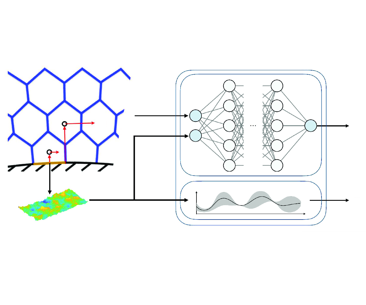
Figure 8 depicts an overview of WMLES and the BFWM-rough. The general steps to build the wall model are as follows.

1. (i) First, the DNS database of minimal-span turbulent channel flows over rough surfaces, as presented in § 2.3, is used to extract mean velocity profiles and wall shear stress for various rough wall geometries.

2. (ii) The inputs to the wall model are constructed as non-dimensional numbers based on the mean velocity profile at two wall-normal locations and roughness geometric parameters. The model is trained using mean velocities from multiple wall-normal locations. This approach is motivated by the fact that, in WMLES, the wall-normal location varies with different grid resolutions and flow conditions, requiring the model to learn this variability.

3. (iii) Wall roughness is assumed to be SGS, meaning that the WMLES grid does not resolve the roughness geometric features. In cases where wall roughness is such that $k_s^+<5$ , the model includes a sensor to switch back to BFWM-smooth from Lozano-Durán & Bae (Reference Lozano-Durán and Bae2023).

4. (iv) The output of BFWM-rough is the local wall-shear stress, which serves as the boundary condition for WMLES at the wall.

5. (v) The relationship between inputs and outputs in BFWM-rough is modelled using feed forward neural network (FNNs).

In the following sections, we discuss the model assumptions, the selection of input and output variables, the architecture of FNNs, and the details of wall model training.

Figure 8. Overview of BFWM-rough for WMLES: for each wall face, the inputs to the wall model include the local flow state and local roughness parameters. The flow state consists of the magnitudes of wall-parallel velocities ( $u_1$ and $u_2$ ) at the centre locations of the first and second off-wall control volumes ( $y_1$ and $y_2$ ), along with the kinematic viscosity $\nu$ . The roughness is assumed to be SGS and known for each control volume attached to the wall. The input roughness parameters are based on the statistical moments of the local roughness height distribution. The output of BFWM-rough is the wall-shear stress vector $\boldsymbol {\tau }_w$ and the confidence score $C\in [0, 1]$ . The wall-shear stress vector is predicted with a FNN, while the confidence score is determined using a GP model. The wall-shear stress vector from BFWM-rough is applied as the local boundary condition to the WMLES.

3.2. Wall model assumptions

We summarize the main modelling assumptions of the BFWM-rough.

1. (i) Building block flow assumption. A finite set of simple flows, based on minimal-span turbulent channel flows over rough surfaces, is sufficient to formulate a generalizable rough-wall model.

2. (ii) Quasi-equilibrium assumption. The near-wall region of complex cases is in a quasi-equilibrium state, i.e. statistically steady flow under mean zero-pressure-gradient effects.

3. (iii) Velocity/shear-stress alignment assumption. The direction of the wall-shear stress vector is aligned with the relative wall-parallel velocity at the first control volume attached to the wall.

4. (iv) Statistical roughness description assumption. A collection of statistical parameters of the rough surface, such as the mean and root-mean-square roughness heights, along with high-order moments of height fluctuations (see table 1), are sufficient to describe the geometrical effects of the surface topology on the wall shear stress.

5. (v) Space/time locality assumption. The relative wall-parallel velocity from the first two contiguous wall-normal control volumes above the wall, combined with (iv), provides enough information to predict the wall shear stress.

6. (vi) Subgrid-scale roughness assumption and outer-layer similarity. The roughness effects on the flow are assumed to be SGS and the only impact of roughness on the resolved scales is through the wall shear stress.

7. (vii) Viscous scaling assumption. The best-performing non-dimensional form of the velocity inputs and the model output is obtained by scaling the variables using the kinematic viscosity and wall-normal distance.

8. (viii) Mean-flow training data assumption. Inputs and outputs samples based on mean velocity profiles and mean wall-shear stress are suitable for training accurate wall models.

Assumptions (i) and (ii) justify the use of the current DNS training database, which targets equilibrium turbulent flows over rough surfaces. Therefore, the application of the BFWM-rough to complex geometries presupposes that the near-wall flow field maintains quasi-equilibrium conditions. Assumptions (iii), (iv) and (v) are adopted primarily for the sake of model simplicity. Incorporating flow information from farther away from the wall could potentially enhance the accuracy of the model, especially for rough surfaces with larger roughness heights. However, this would also increase the complexity of the model when dealing with unstructured grids in realistic geometries. Similarly, the use of roughness statistics instead of detailed local topography simplifies the model, akin to the use of $k_s$ in other approaches. Assumption (vi) is supported by previous observations from the literature (Raupach et al. Reference Raupach, Antonia and Rajagopalan1991) and by the Townsend’s outer-layer similarity hypothesis (Townsend Reference Townsend1976), which has been confirmed by multiple studies (Flack et al. Reference Flack, Schultz and Shapiro2005; Flores & Jimenez Reference Flores and Jimenez2006; Leonardi & Castro Reference Leonardi and Castro2010; Mizuno & Jiménez Reference Mizuno and Jiménez2013; Chung et al. Reference Chung, Monty and Ooi2014; Chan et al. Reference Chan, MacDonald, Chung, Hutchins and Ooi2015; Lozano-Durán & Bae Reference Lozano-Durán and Bae2019a ). The viscous scaling from assumption (vii) is appropriate for the flow scenarios addressed in this study but may become inaccurate under conditions with significant pressure gradients or compressibility effects. The rationale behind assumption (viii) is that the fluctuations of the flow are less critical compared with the mean quantities for predicting the mean wall shear stress. Consequently, the training dataset relies on average flow values from DNS, with added Gaussian noise to improve the robustness of the model.

3.3. Input and output variables

The goal of this section is to select the non-dimensional input variables for the wall model that are most informative for predicting the wall shear stress across the entire training dataset. The input variables include both flow variables and roughness topography parameters. The variables $y_1$ and $y_2$ denote the wall-normal distances to the centres of the first and second control volumes off the wall, respectively (as shown in figure 8), and are related to the WMLES grid resolution by $y_1 \approx \triangle /2$ . The magnitudes of the corresponding wall-parallel velocities relative to the wall at $y_1$ and $y_2$ are $u_1=(u_s(y_1)^2+w_s(y_1)^2)^{1/2}$ and $u_2=(u_s(y_2)^2+w_s(y_2)^2)^{1/2}$ , where $u_s$ and $w_s$ are samples generated as detailed below. Three different grid resolutions, $\triangle /\delta = 1/20, 1/10, 1/5$ , are included in the generation of data for the input and output variables. The grid resolutions correspond to the condition where the first off-wall grid point lies within the buffer layer or the logarithmic layer, which aligns with typical grid resolutions in WMLES for engineering applications. The candidate input variables considered can be organized into five categories:

1. 1) roughness parameters,

   (3.2) \begin{align} \frac {k_{avg}}{R_a}, \frac {k_{c}}{R_a}, \frac {k_{t}}{R_a}, \frac {k_{rms}}{R_a}, S_k, K_u, ES, P_o, I, \frac {L_{cor}}{R_a}, \lambda _f; \end{align}

2. 2) products of roughness parameters,

   (3.3) \begin{align} ES^2, S_k^2, ES S_k, ES K_u; \end{align}

3. 3) roughness height scaled by $y_1$ ,

   (3.4) \begin{align} \frac {k_{avg}}{y_1},\quad \frac {k_{c}}{y_1},\quad \frac {k_{t}}{y_1},\quad \frac {k_{rms}}{y_1},\quad \frac {y_1}{R_a}; \end{align}

4. 4) products of non-dimensional roughness parameters and roughness height scaled by $y_1$ ,

   (3.5) \begin{align} \frac {S_kk_{avg}}{y_1},\quad \frac {K_uk_{avg}}{y_1},\quad \frac {ES k_{avg}}{y_1},\quad \frac {P_ok_{avg}}{y_1},\quad \frac {I k_{avg}}{y_1},\\ \frac {S_kk_{rms}}{y_1},\quad \frac {K_uk_{rms}}{y_1},\quad \frac {ES k_{rms}}{y_1},\quad \frac {P_ok_{rms}}{y_1},\quad \frac {I k_{rms}}{y_1}; \end{align}

5. 5) local Reynolds number at $y_1$ and $y_2$ ,

   (3.6) \begin{align} \frac {u_1y_1}{\nu },\quad \frac {u_2y_2}{\nu }. \end{align}

The samples for $u(y_i)$ and $w(y_i)$ are generated based on a Gaussian distribution $\mathcal {N} [ \mu , \sigma ^2 ]$ with mean $\mu$ and variance $\sigma ^2$ as

(3.7) \begin{equation} u_s(y_i) \sim \mathcal {N}\left [U(y_i),u_{rms}^2(y_i)\right ], \quad w_s(y_i) \sim \mathcal {N}\left [W(y_i),w_{rms}^2(y_i)\right ], \end{equation}

where $U(y_i)$ and $W(y_i)$ are the DNS streamwise and spanwise mean velocities, and $u_{rms}(y_i)$ and $w_{rms}(y_i)$ are the DNS root-mean-squared streamwise and spanwise velocity fluctuations at $y_i$ (with $i=1,2$ ). Products of roughness parameters are also included in categories 2) and 4) as inputs to facilitate model training. Although the FNN can uncover nonlinear relationships between inputs and outputs, it was observed that incorporating quadratic relationships between roughness parameters enabled the training of higher-performing models with less data.

The non-dimensional output of the wall model is

(3.8) \begin{equation} \tilde {\tau }_w=\frac {\tau _{w,s}y_1}{\nu u_1}, \end{equation}

where the scaling factor $\nu u_1/y_1$ represents the naive estimation of the wall shear stress using finite differences. The values of $\tau _{w,s}$ are generated based on a Gaussian distribution $\tau _{w,s} \sim \mathcal {N} [ \langle \tau _w\rangle , \tau _{w,rms}^2 ]$ , where $\langle \tau _w\rangle$ is the mean wall-shear stress calculated from DNS, and $\tau _{w,rms}$ is computed based on the correlation $\tau _{w,rms}/\langle \tau _w\rangle = 0.298 + 0.018\ln Re_{\tau }$ (Örlü & Schlatter Reference Örlü and Schlatter2011). As discussed in § 3.2, the main goal of the current wall model is to correctly predict mean flow quantities. It was found that this approach facilitates the training of more robust models than the use of actual instantaneous DNS values for velocities and wall shear stress.

We aim to select the best-performing input variables from all the candidates defined above. To that end, we use the ‘minimum redundancy maximum relevance’ (MRMR) algorithm to aid the finding of the optimal set of the input features (Ding & Peng Reference Ding and Peng2005; Peng et al. Reference Peng, Long and Ding2005). The MRMR algorithm is designed to rank input variables by considering both their relevance to the output and their redundancy with respect to each other. This helps improve the accuracy of the model and reduce overfitting by eliminating unnecessary inputs. Here, we use the MRMR algorithm to determine the order in which input features will be tested when training candidate models in the following section.

The relevance and redundancy are computed using mutual information, which measures the amount of information shared between variables. The mutual information $I$ between a pair of random variables $(\phi , \psi )$ is defined as

(3.9) \begin{equation} I(\phi ,\psi ) = \iint {PDF}(\phi ,\psi )\log \Biggl ( \frac {{PDF}(\phi ,\psi )}{{PDF}(\phi ){PDF}(\psi )} \Biggr )\mathrm {d}\phi \mathrm {d}\psi , \end{equation}

where ${PDF}(\phi ,\psi )$ is the joint PDF of $\phi$ and $\psi$ , and ${PDF}(\phi )$ and ${PDF}(\psi )$ are the marginal PDFs of $\phi$ and $\psi$ , respectively. The MRMR algorithm ranks features by evaluating the importance score (also known as ‘mutual information quotient’) of an input $\phi _{in}$ ,

(3.10) \begin{equation} {MIQ}_{\phi _{in}} = \frac {V_{\phi _{in}}}{W_{\phi _{in}}}, \end{equation}

where $V_{\phi _{in}}$ is the relevance of the input feature $\phi _{in}$ with respect to the output variable $\phi _{out}$ ,

(3.11) \begin{equation} V_{\phi _{in}} = I(\phi _{in},\phi _{out}) \end{equation}

and $W_{\phi _{in}}$ is the redundancy of the input feature $\phi _{in}$ with respect to the rest of input features $\psi _{in}$ ,

(3.12) \begin{equation} W_{\phi _{in}} = \frac {1}{|\textbf {S}|}\sum _{\psi _{in} \in \textbf {S}} I(\phi _{in},\psi _{in}), \end{equation}

where $|\textbf {S}|$ is the number of features in the set of the input variables $\textbf {S}$ maximizing ${MIQ}_{\phi _{in}}$ . Higher relevance indicates a stronger association with the output, while lower redundancy implies less similarity between inputs.

We use MRMR to identify a subset of input variables that collectively maximize relevance to the target while minimizing redundancy among the selected inputs. Table 5 displays the sequence of the candidate input features informed by the MRMR importance scores in descending order, with the top-ranked inputs being the most informative for predicting the output. The results in table 5 suggests that the local Reynolds numbers, $u_1y_1/\nu$ and $u_2y_2/\nu$ , along with the roughness features $k_{rms}/R_a$ and $ES^2$ , contain the most relevant information for the wall model. It is interesting that the ranking does not prioritize $S_k$ , which has traditionally been a key ingredient in models and correlations for predicting $k_s$ . However, as shown in figure 4, $S_k$ is strongly correlated with $k_{rms}/R_a$ in the present roughness database, where $k_{rms}/R_a$ is the second most important input feature in the ranking. Thus, the effect of $S_k$ is effectively accounted for by including $k_{rms}/R_a$ .

Table 5. Ranking of candidate input variables for the wall model according to MRMR importance score in descending order.

3.4. Wall model training

The order of inputs provided by the ranking in table 5 is used in this section to determine the number of model inputs. An FNN is used to parameterize the relationship between inputs and outputs. The layers are connected using hyperbolic tangent sigmoid transfer functions as the activation function except for the last layer, which is connected with rectified linear units. The training algorithm utilized is gradient descent with momentum and adaptive learning rate backpropagation (Yu & Liu Reference Yu and Liu2002). A total of 192 cases of turbulent channel flows are randomly divided into training dataset (70 % of the total), validation dataset (15 % of the total) and testing dataset (15 % of the total). The training dataset is used to develop a candidate BFWM-rough model; the validation dataset, while not used for parameter estimation, provides the stopping criterion during training to prevent overfitting and enhance the generalizability of the model. The model architecture – including the number of hidden layers and neurons – and hyperparameters are optimized based on performance metrics from the validation dataset. The testing dataset, not involved in the training process, serves as an independent set of cases to assess the performance of BFWM-rough on untrained scenarios.

To find the best-performing model, different numbers of input features are tested according to the order presented in table 5. Note that this ranking is key to limit the number of possible input combinations. For each number of inputs, 100 random splits of the training, validation and testing datasets are conducted. For each split, the optimal number of hidden layers and neurons per layer is determined through a grid search. The number of hidden layers and neurons per layer considered in the grid search ranges from 3 to 6 and from 5 to 20, respectively. The optimal model for each combination of inputs is then determined based on the minimum $L_2$ -norm error over the entire training, validation and testing datasets from the 100 random splits. A total of 8000 central processing unit hours were taken to obtain the optimal wall model.

The errors for different candidate wall models are plotted against the number of inputs in figure 9. The results show that the wall model requires at least five non-dimensional inputs to achieve errors below 10 %. A less significant reduction in error, from 8 % to 4.6 %, is observed with a higher number of inputs after the fifth ranked input. As an interesting observation, it was not possible to train wall models with errors below 10 % without including roughness parameters non-dimensionalized by the grid size.

Table 6. Range of applicability for BFWM-rough for SGS roughness: ratio of roughness height parameters to the grid size of the training dataset.

Figure 9. Apriori $L_2$ -norm error in the prediction of $\tilde {\tau }_w$ as function of the number of input features as ranked in table 5. The inset shows the errors when the number of inputs ranges from 5 to 32.

Figure 10. Scatter plot of regression results of actual $\tilde {\tau }_w$ and predicted $\tilde {\tau }_w$ for BFWM-rough. The results are plotted for three grid resolutions: (a) $\triangle /\delta =1/20$ ; (b) $\triangle /\delta =1/10$ ; (c) $\triangle /\delta =1/5$ .

According to the Buckingham- $\pi$ theorem (Buckingham Reference Buckingham1914), the number of dimensionless numbers ( $\pi$ terms) required to uniquely determine the wall shear stress in the rough-wall channel simulations equals the total number of parameters needed to set up the cases minus the independent fundamental units. In this study, there are seven parameters: $U_c$ (mean centreline velocity), $\delta$ , $\nu$ , $k_{rms}$ , $H$ , $H_f$ and $\kappa _0$ . The number of fundamental units is two (length and time). Therefore, a total of five dimensionless numbers is required to completely specify the case, and hence the wall shear stress. This implies that any model aiming to accurately predict the wall shear stress is expected to require five non-dimensional inputs. This might explain why the model error drops significantly after five inputs. In practice, the non-dimensional inputs available to the wall model do not include global parameters of the case (such as $U_c$ and $\delta$ ). Instead, local quantities are used as proxies. For that reason, adding more inputs can still inform the model predictions.

Based on the results shown in figure 9, the model with 23 inputs is selected as the BFWM-rough model. This model was chosen because it has the minimum number of inputs while maintaining an $L_2$ -norm error below 5 %. The corresponding FNN comprises five hidden layers with 15 neurons per layer. The $L_2$ -norm error for BFWM-rough is 4.76 % across all datasets. As an example, regression results for three different grid resolutions are illustrated in figure 10. It is also useful to evaluate the range of applicability of BFWM-rough in terms of typical roughness heights relative to the WMLES grid resolution. The ratio of roughness height parameters in the training database to the training grid size is summarized in table 6. The BFWM-rough covers a peak-to-valley roughness height $k_c$ from 0.38 $\triangle$ to 3.55 $\triangle$ , and a root-mean-square roughness height $k_{rms}$ from 0.04 $\triangle$ to 0.56 $\triangle$ . In WMLES scenarios characterized by higher ratios (i.e. finer grid resolutions relative to typical roughness element sizes) it may be more accurate to geometrically resolve the roughness with the WMLES mesh and use a wall model for smooth surfaces. The aposteriori performance of BFWM-rough is assessed in actual WMLES in § 4.

3.5. Confidence score

A GP model, similar to the one introduced for AL in § 2.2, is used to calculate a confidence score for the roughness topology. The main objective is to identify potential deficiencies in the BFWM-rough when applied to surfaces with roughness features that differ significantly from those in the training dataset. The GP model is trained on all cases considered for BFWM-rough, but it only utilizes the non-dimensional roughness parameters as inputs. The confidence score is defined as $C = min \{\sigma ^2_{tr}/\sigma ^2, 1\}$ , where $\sigma ^2_{tr}$ is the mean prediction variance of the GP model over the training dataset, and $\sigma ^2$ is the predictive variance of the case for which the confidence is computed. Note that the confidence score provides an assessment only of the roughness geometry and does not account for the flow conditions. When $\sigma ^2_{tr} \approx \sigma ^2$ , then $C \approx 1$ and confidence in the roughness geometry is high. This indicates that the geometric properties of the roughness considered are similar to those the BFWM-rough was trained on. Conversely, large uncertainty in the roughness surface properties will increase $\sigma ^2$ , thereby lowering the confidence score $C \ll 1$ . In those cases, the prediction from BFWM-rough might be subject to significant errors.

4.1. Comparison with existing rough-wall models

The performance of BFWM-rough is compared with existing models in the literature through apriori testing. Five models are considered, and their functional forms are summarized in table 7. Note that previous models predict either the roughness function $\triangle U^+$ or the equivalent sand-grain roughness height $k_s^+$ , whereas BFWM-rough predicts the wall shear stress. We use $\triangle U^+$ to enable comparisons across different models. For models based on correlations for $k_s^+$ , the predicted roughness function $\triangle U^+_{pred}$ is computed based on (2.10). For BFWM-rough, $\triangle U^+_{pred}$ is computed according to the equation $\triangle U^+=U_s^+-U_r^+$ in the logarithmic layer (Flack & Schultz Reference Flack and Schultz2010). This equation can be rewritten in the following formulation to relate $\triangle U^+$ with the predicted wall-shear stress from BFWM-rough:

(4.1) \begin{equation} \triangle U_{pred}^+ = U_{s}^+\left(1-\sqrt {\frac {\tau _{w,s}}{\tau _{w,r}}}\frac {U_{r}}{U_{s}}\right), \end{equation}

where $\tau _{w,r}$ is the predicted wall-shear stress from BFWM-rough, $\tau _{w,s}$ is the wall-shear stress from the DNS of smooth-wall channel flow, and $U_s$ and $U_r$ are obtained from the mean velocity profiles of DNS for smooth- and rough-wall channel flows, respectively. The equation assumes that $U_s^+$ , $\tau _{w,s}$ and $U_r$ are the true values obtained from DNS, while $\tau _{w,r}$ is derived from the model prediction. This establishes an apriori relationship between $\tau _{w,r}$ and $\triangle U^+$ .

Figure 11. Comparison with rough-wall models from table 7 on the overall 192 rough cases in § 3.4: $(a)$ model for $k_s^+$ from Flack et al. (Reference Flack, Schultz and Barros2020); $(b)$ model for $k_s^+$ from Kuwata & Kawaguchi (Reference Kuwata and Kawaguchi2019); $(c)$ model for $\triangle U^+$ from Chan et al. (Reference Chan, MacDonald, Chung, Hutchins and Ooi2015); $(d)$ model for $\triangle U^+$ from De Marchis et al. (Reference De Marchis, Saccone, Milici and Napoli2020); $(e)$ model for $\triangle U^+$ from Bornhoft et al. (Reference Bornhoft, Jain, Bose and Moin2024); $(f)$ results from the BFWM-rough. Here red circle, Gaussian roughness; blue cross, Weibull roughness.

The performance of different models for Gaussian and Weibull roughness is shown in figure 11. The correlation proposed by Flack et al. (Reference Flack, Schultz and Barros2020) provides good predictions for Gaussian roughness with high $ES$ and Weibull roughness with low $ S_k$ , as shown in figure 11(a). This aligns with the assertion from Flack et al. (Reference Flack, Schultz and Barros2020) that this correlation does not adequately capture wavy surfaces with low $ ES $ or surfaces with high positive skewness. A similar correlation proposed by Kuwata & Kawaguchi (Reference Kuwata and Kawaguchi2019) improves predictions for Gaussian roughness with negative $ S_k$ (figure 11 b), although it still overestimates most Weibull roughness with high $ S_k$ . This may be due to the fact that the correlation was developed for rough surfaces with moderate skewness $(-1 \lt S_k \lt 1)$ . The correlation proposed by Chan et al. (Reference Chan, MacDonald, Chung, Hutchins and Ooi2015) (figure 11 c) provides accurate predictions for Weibull roughness with positive $ S_k$ but overpredicts drag for both Gaussian roughness and Weibull roughness with negative $ S_k$ . De Marchis et al. (Reference De Marchis, Saccone, Milici and Napoli2020) found a linear-log correlation between $ \triangle U^+$ and $ ES \cdot k_{rms}^+$ , which overestimates Gaussian roughness and Weibull roughness with negative $ S_k$ while underpredicting Weibull roughness with high positive $ S_k$ , as shown in figure 11(d). Figure 11(e) displays results from a correlation with a more comprehensive treatment of roughness parameters, proposed by Bornhoft et al. (Reference Bornhoft, Jain, Bose and Moin2024). This model offers improved predictions compared with the previously discussed models; however, it still overpredicts Gaussian roughness and shows significant errors for certain Weibull roughness profiles. Finally, results for BFWM-rough are shown in figure 11(f), where it provides the most accurate predictions for both training and testing rough cases. For fairness, it should be noted that our model achieves the highest accuracy partly because it was specifically trained on Gaussian and Weibull roughness. However, it is also worth emphasizing that BFWM-rough can be retrained with an expanded roughness database using the workflow outlined in this study.

4.2. Rough-wall turbulent channel flow

The performance of BFWM-rough is evaluated first in WMLES of turbulent channel flows. The WMLES equations are solved using staggered second-order finite differences and a fractional-step method with a third-order Runge–Kutta time advancement scheme (Bae et al. Reference Bae, Lozano-Durán, Bose and Moin2019; Lozano-Durán & Bae Reference Lozano-Durán and Bae2019a ,Reference Lozano-Durán and Baeb). The dynamic Smagorinsky model (Germano et al. Reference Germano, Piomelli, Moin and Cabot1991; Lilly Reference Lilly1992) is used as the SGS model. The simulations are conducted by fixing the Reynolds number based on the mean centreline velocity, $Re_c = U_c \delta /\nu$ . The streamwise, wall-normal and spanwise lengths of the computational domain are $2\pi \delta$ , $2\delta$ and $\pi \delta$ , respectively. Six grid resolutions are considered, all of them with equal grid size in each spatial direction: $\triangle /\delta = 1/5, 1/8, 1/10, 1/15, 1/20$ and $1/30$ . The simulations were carried out for 30 eddy turnover times after transients.

Hereafter, we use the term ‘untrained’ (or testing) to indicate that the model was never trained for that particular rough surface, rough Reynolds number ( $k_s^+$ ) and/or grid resolution. The term ‘trained’ is used when the model was explicitly trained for that condition. The four categories of cases examined are as follows:

1. (i) trained Gaussian/Weibull rough surfaces;

2. (ii) untrained Gaussian/Weibull rough surfaces;

3. (iii) untrained bimodal Gaussian rough surfaces;

4. (iv) untrained ellipsoidal, sinusoidal, Fourier-mode and sand-grain rough surfaces from Jouybari et al. (Reference Jouybari, Yuan, Brereton and Murillo2021).

Cases in (i), (ii) and (iii) are evaluated at untrained grid resolutions and untrained $k_s^+$ , whereas cases in (iv) are only conducted for untrained $k_s^+$ .

Table 8. Relative errors (in %) of $\tau _w$ for the trained Gaussian/Weibull rough surfaces at trained/untrained grid resolutions and untrained Reynolds numbers. Note that these cases are from the testing dataset in § 3.4. The relative error is computed based on the predicted value from the BFWM-rough and the actual value from DNS in turbulent channel flows. The table shows case name, $Re_{\tau }$ , and $\hat {k}_s^+$ .

4.2.1. Trained Gaussian/Weibull rough surfaces

Figure 12. Mean velocity profiles for DNS (line) and WMLES (symbols) of turbulent channel flows for selected test cases: (a) WB13 at $Re_\tau =720$ ; (b) WB06 at $Re_\tau =360$ ; (c) GS03 at $Re_\tau =720$ ; (d) WB05 at $Re_\tau =360$ ; (e) GS14 at $Re_\tau =540$ ; (f) GS18 at $Re_\tau =1000$ . The roughness geometries are visualized with a section of $\delta$ in $x$ and $0.5\delta$ in $z$ . Three grid resolutions are visualized: $\triangle /\delta =1/20$ ( $\circ$ ); $\triangle /\delta =1/15$ ( $+$ ); $\triangle /\delta =1/30$ ( $\times$ ).

Six cases from the testing datasets in § 3.4, spanning both fully and transitionally rough regimes, are selected for evaluation: WB13- $Re_{\tau }=720$ , WB06- $Re_{\tau }=360$ , GS03- $Re_{\tau }=720$ , WB05- $Re_{\tau }=360$ , GS14- $Re_{\tau }=540$ and GS18- $Re_{\tau }=1000$ . Note that the six rough surfaces are seen during the training process, however, they are evaluated at untrained rough Reynolds numbers. The cases are also examined for three training grid sizes ( $\triangle /\delta =1/20, 1/10, 1/5$ ) and three testing grid sizes ( $\triangle /\delta =1/30, 1/15, 1/8$ ). The grid sizes $\triangle /\delta =1/15$ and $\triangle /\delta =1/8$ fall within the range of the training grids, while $\triangle /\delta =1/30$ is outside this range.

The apriori and aposteriori errors for the predicted wall shear stress are listed in table 8. The apriori mean error is 6 % with a standard deviation of 7 %. The errors range from 0 % to 30 %, with the latter occurring for rough surfaces with Weibull distributions at the finest grid resolution considered ( $\triangle /\delta =1/30$ ). This discrepancy could be attributed to two factors. First, the characterization of Weibull surfaces requires more parameters than Gaussian roughness, complicating predictions due to the increased dimensionality of the input space. Second, the finest grid resolution falls outside the bounds of the training set. These factors combined make Weibull surfaces at fine grid resolutions more susceptible to inaccurate results due to model extrapolation. The mean aposteriori error is 9 %, with a standard deviation of 5 %. In some instances, aposteriori errors are lower than apriori errors. However, this apparent improvement is due to error cancellation arising from external errors in the SGS model.

The streamwise mean velocity profiles from WMLES are plotted and compared with DNS results in figure 12. To facilitate the visualization of near-wall errors from WMLES, the mean velocity $U$ is normalized by $U_c$ instead of $u_\tau$ . The wall-normal distance is non-dimensionalized by $(y-d)/\delta$ . Three grid resolutions are shown: $\triangle /\delta =1/20$ , $\triangle /\delta =1/15$ and $\triangle /\delta =1/30$ . The agreement between DNS and WMLES is within 5 %, demonstrating the capability of BFWM-rough in predicting the mean velocity profiles for both fully and transitionally rough cases. It is important to note that the SGS model plays a crucial role in predicting the mean velocity profile. Therefore, most of the errors observed in figure 12 are likely dominated by deficiencies in the SGS model rather than internal errors from BFWM-rough.

4.2.2. Untrained Gaussian/Weibull rough surfaces

Figure 13. Confidence score for each surface in the roughness repository. Surface indices 1–50 are Gaussian roughness, and surface indices 51–100 are Weibull roughness. The training cases are coloured in green. The four cases with the smallest $C$ (coloured in red) are selected for evaluation of BFWM-rough.

We evaluate BFWM-rough on surfaces from the roughness repository whose geometrical features are not included in the training process. Additionally, these cases contain untrained $k_s$ and are assessed in untrained grid resolutions. To identify the most challenging cases, we use the confidence score $C$ introduced in § 3.5 to select rough surfaces with the lowest confidence for evaluation. Figure 13 displays the confidence scores for each surface in the roughness repository. As expected, the confidence levels for all training cases (coloured in green) are around 100 %. The confidence scores for the untrained rough surfaces range from 45 % to 90 %. The four cases with the lowest $C$ scores (WB14, WB15, WB16 and WB17, coloured in red) are selected for evaluation of BFWM-rough. The geometrical parameters of these four surfaces are summarized in table 9.

Table 9. Roughness parameters of Weibull and Bimodal rough surfaces for model evaluation.

Figure 14. Apriori error variation of wall-shear stress against $k_s^+$ . Untrained Weibull and Bimodal rough surfaces are tested for $Re_{\tau }=180, 360, 540, 720, 900$ and $1000$ with trained and untrained grid resolutions, as shown by the symbols with increasing $k_s^+$ . The error is given as a fraction. Note that these selected untrained rough surfaces are the most challenging test cases with the least confidence scores.

Figure 15. Aposteriori error variation of wall-shear stress against $k_s^+$ . Untrained Weibull and Bimodal rough surfaces are tested in WMLES of turbulent channel flow at $Re_{\tau }=180, 360, 540, 720, 900$ and $1000$ with trained and untrained grid resolutions, as shown by the symbols with increasing $k_s^+$ . The error is given as a fraction, and the legend is the same as figure 14.

The errors in ${\tau }_w$ are shown in figures 14 and 15 for both apriori and aposteriori testing across different training and testing grid resolutions. The streamwise mean velocity profiles from WMLES are plotted in figure 16 and compared with those from DNS for some selected cases. We should note that these selected untrained rough surfaces are the most challenging test cases with the least confidence scores. Generally, in apriori testing, BFWM-rough tends to overpredict drag in the transitionally rough regime and underpredict drag in the fully rough regime. However, this pattern is not always seen in aposteriori testing due to possible error cancellation. Both apriori and aposteriori errors decrease with increasing $k_s^+$ in the transitionally rough regime and stabilize in the fully rough regime. The BFWM-rough exhibits apriori errors ranging from $-20\,\%$ to 40 % across the training grids, and errors within 25 % in aposteriori testing due to error cancellation. As summarized in table 10, the mean and standard deviation of drag prediction errors on Weibull roughness are within 8 % and 10 %, respectively. In the transitionally rough regime, the mean prediction error is smaller than in the fully rough regime, but the standard deviation is larger. The error variation in aposteriori testing shows a similar trend with increasing $k_s^+$ , with values generally lower than in apriori testing. The best predictions are achieved for WB17, with errors mostly under 10 % in both apriori and aposteriori testing across all grid resolutions. In contrast, WB16 shows the largest errors, likely due to its high $k_{rms}$ and large correlation wavelength (small $ES$ ), which fall outside the characteristics of Weibull rough cases in the training database.

Figure 16. Mean velocity profiles for DNS (line) and WMLES (symbols) of turbulent channel flows at $Re_{\tau }=1000$ with test Weibull surfaces: (a) WB14; (b) WB15; (c) WB16; (d) WB17. The roughness geometries are visualized with a section of $\delta$ in $x$ and $0.5\delta$ in $z$ . Three grid resolutions are visualized: $\triangle /\delta =1/20$ ( $\circ$ ); $\triangle /\delta =1/15$ ( $+$ ); $\triangle /\delta =1/30$ ( $\times$ ).

Table 10. Model evaluation in the transitionally and fully rough regimes, demonstrated by the mean and standard deviation (in %) of the errors in the testing untrained Weibull and Bimodal rough cases (crossing different $Re_{\tau }$ with training and testing grids).

4.2.3. Untrained bimodal Gaussian rough surfaces

In this section, BFWM-rough is evaluated on rough surfaces with a bimodal Gaussian distribution. The goal is to assess the performance of BFWM-rough on a new roughness type that shares some similarities with the surfaces included in the roughness repository but does not follow the same generation process. The selection of bimodal Gaussian roughness is motivated by the presence of engineering surfaces, which are frequently generated by successive processes or multiple factors. This introduces two or more different modal roughness distributions into the final surface (Peng & Bhushan Reference Peng and Bhushan2000). One example of a bimodal roughness distribution is observed in ice accretion on airfoils (Bornhoft et al. Reference Bornhoft, Jain, Goc, Bose and Moin2022). The bimodal Gaussian distributions are constructed by combining two Gaussian distributions according to (Peng & Bhushan Reference Peng and Bhushan2000)

(4.2) \begin{equation} {PDF}_B(\tilde {k}) {=} {PDF}_G(\tilde {k};0,1){+}{PDF}_G(\tilde {k};\mu _G,\sigma ^2_G){-} {PDF}_G(\tilde {k}; 0,1) {PDF}_G(\tilde {k};\mu _G,\sigma ^2_G), \end{equation}

where ${PDF}_B(\tilde {k})$ is the PDF of the bimodal distribution, ${PDF}_G(\tilde {k};0,1)$ is a normal distribution and ${PDF}_G(\tilde {k};\mu _G,\sigma ^2_G)$ is the Gaussian distribution with randomized mean $0 \lt \mu _G \lt 0.5$ and randomized variance $0 \lt \sigma ^2_G \lt 0.5$ . The power spectra is specified in the same way as described in § 2.1. The resulting surface map is then scaled from 0 to the root mean square height normalized by the channel half-height $k_{rms}/\delta$ , whose values are randomly chosen in the range of $0.005\lt k_{rms}/\delta \lt 0.030$ . A total of 23 bimodal rough surfaces are generated. Their confidence scores, shown in figure 17, are approximately 50 %. The most challenging surfaces for evaluation are identified as those with the lowest confidence score: BM01, BM02, BM03 and BM04 (where BM refers to bimodal roughness). Their roughness parameters are listed in table 9.

Figure 17. Confidence scores for 23 bimodal rough surfaces not included in the roughness repository. The four cases with the smallest $C$ (coloured in red) are selected for evaluation of BFWM-rough.

The performance of BFWM-rough for BM01, BM02, BM03 and BM04 is shown in figures 14 and 15. Similar error variations as Weibull roughness are observed with increasing $k_s^+$ . Table 10 shows that the mean and standard deviation of errors for Bimodal roughness are larger than Weibull in the transitionally rough regime, but comparable to Weibull in the fully rough regime. It is also worth noting that for both Weibull and Bimodal roughness, the errors are generally smaller in aposteriori testing than apriori testing due to the internal and external error cancellation. Despite the mean errors being larger than in the previous sections, the results still demonstrate that BFWM-rough can offer reasonable predictions for new roughness types as long as these follow similar distributions to those it was trained for. The largest errors are obtained for BM04. The primary distinction between BM04 and the other three surfaces, as well as surfaces in the training database, is the combination of large negative $S_k$ and large effective slopes for BM04. These roughness features can lead to less drag; however, since the training database lacks this information, the wall model results in an overestimation of the wall shear stress for BM04. The mean velocity profiles of WMLES compared with DNS are shown in figure 18. The improved agreement with the DNS results for BM04 at the grid resolutions of $\triangle /\delta =1/20$ and $\triangle /\delta =1/30$ is due to error cancellation in aposteriori evaluation.

Figure 18. Mean velocity profiles for DNS (line) and WMLES (symbols) of turbulent channel flows at $Re_{\tau }=1000$ with bimodal surfaces: $(a)$ BM01; $(b)$ BM02; $(c)$ BM03; $(d)$ BM04. The roughness geometries are visualized with a section of $\delta$ in $x$ and $0.5\delta$ in $z$ . Three grid resolutions are visualized: $\triangle /\delta =1/20$ ( $\circ$ ); $\triangle /\delta =1/15$ (+); $\triangle /\delta =1/30$ (x).

4.2.4. Untrained rough surfaces from Jouybari et al. (Reference Jouybari, Yuan, Brereton and Murillo2021)

The final cases analysed are the roughness types from Jouybari et al. (Reference Jouybari, Yuan, Brereton and Murillo2021). The goal is to assess the performance of BFWM-rough on surfaces with topologies significantly different from the roughness repository used for training. A total of 42 rough surfaces are evaluated (labelled from C01 to C42), including 27 fully rough and 15 transitionally rough cases. The cases comprise ellipsoidal, sinusoidal, Fourier-mode and sand-grain roughnesses. The topology of some of the surfaces is shown in figure 19. The exact $\tilde {\tau }_w$ for all 42 rough cases is obtained from the DNS of turbulent channel flows at $Re_{\tau }=1000$ as reported by Jouybari et al. (Reference Jouybari, Yuan, Brereton and Murillo2021).

Figure 19. (a) Confidence score for each rough surface and (b) apriori relative error (in %) of predicted $\tilde {\tau }_w$ using the BFWM-rough and actual $\tilde {\tau }_w$ from DNS of Jouybari et al. (Reference Jouybari, Yuan, Brereton and Murillo2021). The cases with the model error within $\pm 30\,\%$ are highlighted in yellow in (a). The dashed lines in (b) denote the error values at $\pm 30\,\%$ . Roughness index 1–42 corresponds to Cases C01–C42 in Jouybari et al. (Reference Jouybari, Yuan, Brereton and Murillo2021). The topology of some of the surfaces is visualized on the right-hand side: ellipsoidal roughness, C04 and C21; surfaces with sinusoidal waves, C29 and C30; roughness generated by Fourier modes, C34 and C39; sandgrain roughness, C31 and C37.

The confidence score for each surface is presented in figure 19(a). Overall, the results demonstrate the capability of the confidence score to identify untrained surfaces. The confidence levels range from 0.35 to 0.45, which are lower than those for the previous test cases involving untrained Weibull and Bimodal roughnesses. The highest confidence scores are found for cases C31 to C42, which correspond to sand-grain roughness and surfaces generated by low-order Fourier modes. These cases share more similarities with the isotropic roughness in the training dataset, explaining their higher confidence scores. The lowest confidence is observed for ellipsoidal roughness (C01 to C24) and roughness with streamwise sinusoidal waves (C25 to C30). This is expected, as the ellipsoidal elements are generated with varying orientations and semiaxis lengths, and the sinusoidal rough surfaces feature only streamwise waves. Both of these roughness types represent strongly anisotropic roughness, differing significantly from the surfaces in the training database.

Apriori relative errors for $\tilde {\tau }_w$ are plotted in figure 19(b). The grid resolution considered is $\triangle /\delta = 1/20$ . Consistent with the evaluation by the confidence score, BFWM-rough tends to perform best for cases C31 to C42. However, the predictions can exhibit errors of up to 30 %, which is significantly higher than the errors reported for previous test cases. The majority of cases from C01 to C30 show errors above 30 %, correlating with their low confidence scores. There are instances where the confidence score is low, yet the errors remain below 30 %. This might be coincidental, and caution should always be exercised for predictions accompanied by low values of the confidence score.

4.3. High-pressure turbine blade with roughness

We assess the performance of BFWM-rough in a HPT with wall roughness. Surface roughness on HPT blades can result from the manufacturing process or in-service degradation, significantly affecting the aerothermal performance of the blade (Nardini et al. Reference Nardini, Jelly, Kozul, Sandberg, Vitt and Sluyter2023). The case selected for evaluation is the VKI LS-89 HPT blade with surface roughness, and the results are compared with previous numerical studies by Jelly et al. (Reference Jelly, Nardini, Rosenzweig, Leggett, Marusic and Sandberg2023) and Nardini et al. (Reference Nardini, Jelly, Kozul, Sandberg, Vitt and Sluyter2023). This case involves laminar–turbulent transition, strong pressure gradient effects, shock waves and vortical wakes. Therefore, it presents a challenging scenario to evaluate the predictive capabilities of WMLES in practical flow conditions involving complex geometries and flow physics.

Our WMLES follows the WRLES set-up from Jelly et al. (Reference Jelly, Nardini, Rosenzweig, Leggett, Marusic and Sandberg2023). The exit Reynolds number is $Re_{ex} = \rho _{ex}U_{ex}C_{ax}/\mu _{\infty } = 590\,000$ , and the exit Mach number is $Ma_{ex}=U_{ex}/c_{\infty }=0.9$ , where $\rho _{ex}$ and $U_{ex}$ are the mean exit density and velocity, respectively. Here $C_{ax}$ is the axial chord length, $\mu _{\infty }$ is the dynamic viscosity of the reference state and $c_{\infty }$ is the acoustic velocity for the reference state. The inflow freestream turbulence is generated by a spanwise array of parallel bars. The turbulence intensity ( $TI$ ) is defined as $TI=1/3({u'_{rms}}^2+{v'_{rms}}^2+{w'_{rms}}^2)$ . The value of $TI$ is set to $8\,\%$ of the axial mean inlet velocity $U_{in}$ by adjusting the distance of the bars upstream of the blade. The total pressure and temperature are specified at the inlet with the characteristic boundary conditions. At the exit, the non-reflective Navier–Stokes characteristic boundary conditions are enforced. The static pressure is prescribed at the exit based on the isentropic Mach number relationships. Periodic boundary conditions are prescribed at the upper, lower and spanwise boundaries. The spanwise extent of the domain is set to $0.4C_{ax}$ , as suggested by Pichler et al. (Reference Pichler, Sandberg, Laskowski and Michelassi2017), to ensure the correct development of the largest inflow turbulence structures.

Figure 20. Visualization of Voronoi control volumes for WMLES of the HPT blade: the whole computational domain with a zoom-in view near the leading edge of the blade.

The mesh generation is based on the Voronoi tessellation of a collection of points. The Voronoi control volumes are visualized in figure 20. The size of the background grid is $\triangle _b=0.0311C_{ax}$ . The grid size near the upstream bars is refined to $({1}/{2})\triangle _b$ with 20 layers, and the flow field near the bars is wall-resolved. As shown in the zoom-in view of figure 20, the grid size near the blade is refined by four levels, and for each level, the grid size is reduced by 50 % with 30 layers. As a result, the minimum grid size near the blade surface is $({1}/{16})\triangle _b=0.00195C_{ax}$ , and the number of control volumes per boundary layer thickness ranges from 0 (at the blade leading edge) to 30 (at the blade trailing edge). The total number of control volumes is $26\,{\times}\,10^6$ .

Two different surface roughness profiles are considered for the blade. The cases, denoted as BS01 and BS02, feature three-dimensional, irregular Gaussian roughness. The key geometrical parameters of the roughness are summarized in table 11, which also includes the confidence scores for both rough surfaces. The confidence scores are $C=0.73$ for BS01 and $C=0.67$ for BS02, indicating that the roughness topologies can potentially be well-predicted by BFWM-rough. The WMLES with BFWM-rough is conducted for both blade surfaces, using the Vreman model (Vreman Reference Vreman2004) as the SGS model. The instantaneous axial velocity field from WMLES with BFWM-rough for roughness BS01 is visualized in figure 21, with the boundary layer transition observable in the zoom-in view. The results are compared with the WRLES results of Jelly et al. (Reference Jelly, Nardini, Rosenzweig, Leggett, Marusic and Sandberg2023) and DNS data of Nardini et al. (Reference Nardini, Jelly, Kozul, Sandberg, Vitt and Sluyter2023) for the same rough surfaces.

Table 11. The key geometrical roughness parameters of the blade surface roughness BS01 and BS02 from Jelly et al. (Reference Jelly, Nardini, Rosenzweig, Leggett, Marusic and Sandberg2023). The last column contains the confidence score of BFWM-rough for BS01 and BS02.

Figure 21. Visualization of the instantaneous axial velocity field normalized by the axial mean inlet velocity $u_{ax}/U_{in}$ for WMLES of the HPT blade. The arrow indicates the location at $99\,\%$ of the axial chord length for probing the mean tangential velocity.

Figure 22 shows the time- and spanwise-averaged skin-friction coefficient $C_f$ for WMLES and DNS. The $C_f$ for a smooth blade obtained from DNS is included as a reference to demonstrate the effects of roughness. The WMLES using an equilibrium wall model with prescribed $k_s$ (denoted by EQWM- $k_s$ ) is also shown in figure 22 for a comparison with BFWM-rough. The value of $k_s$ is taken to be $k_s=\alpha k_{rms}$ , with $\alpha$ set to a constant value. Hama (Reference Hama1954) suggested a scaling factor of $\alpha =5$ for Gaussian roughness. However, this is not always accurate as the other roughness parameters such as $ES$ and $L_{cor}/R_a$ may also affect the value of $k_s$ . For example, we found that $\alpha$ ranges from 3.5 to 6.5 for Gaussian roughness in our DNS database. For that reason, the EQWM- $k_s$ is tested within the range $\alpha =3{\sim}7$ . The shaded area in figure 22 shows the variation of the results by EQWM- $k_s$ for the range of values considered for $k_s$ .

On the pressure side (PS) of the blade, the increase in $C_f$ is due to the boundary layer transition, which occurs in the trailing-edge region. The increase in roughness on the PS of the blade is accurately captured by BFWM-rough and EQWM- $k_s$ for the two rough surfaces. The results also indicate that the skin friction on the PS of the blade is only mildly sensitive to the value of $k_s$ . The roughness effects are more significant on the suction side (SS) of the blade. The sharp increase in skin friction corresponds to the laminar-to-turbulent transition of the boundary layer, with larger roughness elements (BS02) triggering an earlier transition compared with the smaller roughness (BS01). Both WMLES with BFWM-rough and EQWM- $k_s$ capture the key trends of the rough wall blade that are absent in the smooth wall case, such as the faster and larger increase in $C_f$ and the second peak after $x/C_{ax}\gt 0.5$ . It is also observed that the BFWM-rough outperforms the EQWM- $k_s$ in the region $0.5\lt x/C_{ax}\lt 0.8$ where the fully developed turbulence occurs in the two rough cases, while the prediction based on EQWM- $k_s$ shows sensitivity to the variation of $k_s$ in this region. In addition, for both BFWM-rough and EQWM- $k_s$ , the value of $C_f$ is overpredicted from $x/C_{ax}=0.7$ to the trailing edge for the two rough cases. This might be related to the interaction of the TBL over the blade with the shock waves within the region $0.7\lt x/C_{ax}\lt 0.9$ . This effect was described by Nardini et al. (Reference Nardini, Jelly, Kozul, Sandberg, Vitt and Sluyter2023), who noted that a normal shock wave is induced by the roughness, with larger roughness magnitude increasing the intensity of normal shock patterns. The presence of shock waves may lead to the formation of shock-induced vortices, and these vortices can interact with the boundary layer, influencing its stability and altering the skin friction pattern. This intricate effect might not be correctly captured by WMLES and multiple factors beyond the wall model (e.g., SGS models and grid resolution) are probably at play.

Figure 22. Time and spanwise-averaged distribution of skin friction coefficient $C_f$ along the axial position of the blade normalized by axial chord length $x/C_{ax}$ . (a) Roughness BS01 and (b) roughness BS02. The DNS results of smooth and rough surfaces are from Nardini et al. (Reference Nardini, Jelly, Kozul, Sandberg, Vitt and Sluyter2023). The blade roughness BS01 and BS02 correspond to cases $k_2^s$ and $k_3^s$ in Nardini et al. (Reference Nardini, Jelly, Kozul, Sandberg, Vitt and Sluyter2023). The shaded area denotes the WMLES with EQWM- $k_s$ , where $k_s=\alpha k_{rms}$ , and $\alpha =3\sim 7$ . Note that $x/C_{ax} \gt 0$ and $x/C_{ax} \lt 0$ correspond to the SS and PS, respectively, with $x/C_{ax} = 0$ locate at the leading edge of the blade.

Figure 23. Mean tangential velocity at $x/C_{ax}=0.99$ normalized by the local freestream velocity $U_t/U_{\infty }$ along the blade-normal direction normalized by axial chord length $y_n/C_{ax}$ . (a) Roughness BS01 and (b) roughness BS02. The WRLES results of smooth and rough surfaces are from Jelly et al. (Reference Jelly, Nardini, Rosenzweig, Leggett, Marusic and Sandberg2023). The shaded area denotes the WMLES with EQWM- $k_s$ , where $k_s=\alpha k_{rms}$ , and $\alpha =3\sim 7$ .

Figure 23 shows the mean tangential velocity profiles close to the trailing edge at the axial location $x/C_{ax}=0.99$ . The results from WMLES are compared with WRLES from Jelly et al. (Reference Jelly, Nardini, Rosenzweig, Leggett, Marusic and Sandberg2023). Although both the smooth- and rough-blade boundary layers have transitioned to turbulence in the trailing-edge region of the SS surface, the flow has yet to reach fully rough conditions (Jelly et al. Reference Jelly, Nardini, Rosenzweig, Leggett, Marusic and Sandberg2023). Figure 23 illustrates that the velocity deficit is generally well captured by the WMLES with BFWM-rough for both rough surfaces considered. For BS01, BFWM-rough slightly overpredicts the velocity deficit, while for BS02, the predictions exhibit high accuracy. These results indicate that BFWM-rough performs well in modelling the integrated momentum deficit along the blade, which is ultimately responsible for the lower-speed mean velocity profiles at the trailing edge. The WMLES with EQWM- $k_s$ also demonstrates good performance for case BS01; however, it clearly underpredicts the velocity deficit for case BS02.