


1 Introduction
Synthetic (non-biological) nanoscale motors have been developed for applications in the biological sciences, including transport of colloidal cargos (Sundararajan et al. Reference Sundararajan, Lammert, Zudans, Crespi and Sen2008; Ye, Diller & Sitti Reference Ye, Diller and Sitti2012), chemical analysis of pollutants (Guix et al. Reference Guix, Orozco, García, Gao, Sattayasamitsathit, Merkoçi, Escarpa and Wang2012; Orozco et al. Reference Orozco, García-Gradilla, D’Agostino, Gao, Cortés and Wang2013) and detection of DNA and other biological molecules (Wu et al. Reference Wu, Balasubramanian, Kagan, Manesh, Campuzano and Wang2010; Campuzano et al. Reference Campuzano, Kagan, Orozco and Wang2011). These motors can also produce emergent dynamics when gathered in large ensembles. Swarming and hydrodynamic synchronisation are but a few aspects of the intriguing dynamics that occurs in these systems (Ibele, Mallouk & Sen Reference Ibele, Mallouk and Sen2009; Xu et al. Reference Xu, Soto, Gao, Dong, Garcia-Gradilla, Magaña, Zhang and Wang2015).
Motion of nanoscale particles can be directed by an external field or can occur autonomously, i.e. the particle acts as a motor. One example of an autonomous nano-motor is a colloidal particle that is driven by osmotic propulsion due to inhomogeneities in its surface properties (Córdova-Figueroa & Brady Reference Córdova-Figueroa and Brady2008). Catalytic motors that operate using fuels such as hydrogen peroxide also lead to autonomous propulsion – by bubble recoil (Fattah et al. Reference Fattah, Loget, Lapeyre, Garrigue, Warakulwit, Limtrakul, Bouffier and Kuhn2011; Loget & Kuhn Reference Loget and Kuhn2011) or chemical gradients (Paxton et al. Reference Paxton, Kistler, Olmeda, Sen, St. Angelo, Cao, Mallouk, Lammert and Crespi2004; Howse et al. Reference Howse, Jones, Ryan, Gough, Vafabakhsh and Golestanian2007; Sánchez, Soler & Katuri Reference Sánchez, Soler and Katuri2015). In contrast, optical and magnetic fields can drive the motion of nanoparticles by the direct forces that these fields impart (Wiel et al. Reference Wiel, Delden, Meetsma and Feringa2005; Saha & Stoddart Reference Saha and Stoddart2007; Tierno et al. Reference Tierno, Golestanian, Pagonabarraga and Sagués2008; Jiang, Yoshinaga & Sano Reference Jiang, Yoshinaga and Sano2010; Fischer & Ghosh Reference Fischer and Ghosh2011). Robotically manoeuvred nanorods that generate localised hydrodynamic vortex traps have also been reported (Petit et al. Reference Petit, Zhang, Peyer, Kratochvil and Nelson2011). A review of the many mechanisms leading to autonomous and directed propulsion of nanoparticles has been conducted by Guix, Mayorga-Martinez & Merkoçi (Reference Guix, Mayorga-Martinez and Merkoçi2014).
Acoustic fields have been used to directly propel particles, i.e. in a prescribed and external manner, leading to wide ranging behaviour. This includes the alignment of elongated rods (Lim, Yao & Chen Reference Lim, Yao and Chen2007) and manipulation of particles into a variety of patterns (Oberti, Neild & Dual Reference Oberti, Neild and Dual2007; Shi et al. Reference Shi, Yazdi, Lin, Ding, Chiang, Sharp and Huang2011). These directed propulsion phenomena are driven first by the time-averaged pressure gradient of the acoustic field which imparts a force on the particles either towards or away from the pressure nodes – this directionality depends on the properties of the particles (King Reference King1934; Eller Reference Eller1968). The particles are then dragged along with the (steady) streaming flow generated by the geometry of the fluid cell, i.e. the particles are moved directly and passively by this (external) secondary flow (Barnkob et al. Reference Barnkob, Augustsson, Laurell and Bruus2012). The particles do not generate their own propulsion.
Recent measurements show that nano and micrometre-scale rods can produce autonomous propulsion in acoustic fields (Wang et al. Reference Wang, Castro, Hoyos and Mallouk2012), i.e. the particles themselves actively generate their propulsive motion rather than being moved passively by an external steady flow. These rods migrate towards a pressure node in a standing acoustic wave where they subsequently exhibit a variety of dynamics, including aggregation, random walks and orbital motion (Ahmed et al. Reference Ahmed, Gentekos, Fink and Mallouk2014; Wang et al. Reference Wang, Li, Mair, Ahmed, Huang and Mallouk2014, Reference Wang, Duan, Zhang, Sun, Sen and Mallouk2015; Rao et al. Reference Rao, Li, Meng, Zheng, Cai and Wang2015; Ahmed et al. Reference Ahmed, Wang, Bai, Gentekos, Hoyos and Mallouk2016). These motors offer a distinct advantage over the autonomous motion of catalytic devices because chemical fuels, which are toxic to many biological systems, are not used. In addition, acoustic fields in the MHz range have been applied extensively in biologically sensitive environments with minimal adverse impact (Litvak, Foster & Repacholi Reference Litvak, Foster and Repacholi2002).
The synthesis process for these nanorods, composed of metal, ensures one of their ends is concave while the other is convex. Originally, Wang et al. (Reference Wang, Castro, Hoyos and Mallouk2012) suggested that this shape variation was causing an asymmetry in the acoustic pressure due to the scattering of the acoustic waves on the surface of the particle, leading to propulsion. However, this hypothesis was later found to be inconsistent with experiments. It predicted the opposite direction of motion to that observed by Ahmed et al. (Reference Ahmed, Gentekos, Fink and Mallouk2014, Reference Ahmed, Wang, Bai, Gentekos, Hoyos and Mallouk2016) – measurements show that particles composed of a single metal always move with their concave end leading. Nadal & Lauga (Reference Nadal and Lauga2014) proposed a mechanism due to the streaming flow generated by a sphere (composed of a single material) with a slight shape perturbation to its surface – this ‘near spherical’ approach facilitates a simple numerical solution. The model, valid in the low acoustic Reynolds number regime (i.e. low frequency, as defined in § 2), predicts autonomous motion based on the nature of the shape perturbations on the sphere’s surface.
In a follow up study, Ahmed et al. (Reference Ahmed, Wang, Bai, Gentekos, Hoyos and Mallouk2016) demonstrated that the propulsion velocity of bimetallic nanorods can be substantially faster than nanorods made of a single metal; the nanorods are composed of two distinct metals occupying each half-length of the rod. When the density difference of the two metals is large, the direction of motion is always observed to be towards the particle’s lighter end. Indeed, motion in the direction of the convex end of the nanorod is reported, in contrast to the nanorods composed of a single metal (discussed above). These measurements therefore show that shape and density asymmetries can produce competing effects, with the particle tending to propel itself with its low density and concave end leading the motion. Importantly, the model of Nadal & Lauga (Reference Nadal and Lauga2014) cannot be used to describe these experimentally reported effects (Ahmed et al. Reference Ahmed, Wang, Bai, Gentekos, Hoyos and Mallouk2016) because the model does not include the effect of density variations in the solid.
The aim of this article is to formulate a general theoretical framework for this phenomenon that can be used to explain its essential physical mechanisms. The previously used assumptions of a nearly spherical and homogeneous density particle in a low acoustic Reynolds number flow (Nadal & Lauga Reference Nadal and Lauga2014) are relaxed – the developed framework is applicable to arbitrarily shaped axisymmetric solids with arbitrary density distributions that are being driven at arbitrary finite frequency. All that is required is solution of the (linear) unsteady Stokes equations, either by analytical or numerical means. This model is then applied to high aspect ratio dumbbell-shaped particles (where analytical results are obtained) and nanorods whose shape mimics the particles reported experimentally (where our framework is implemented numerically). This sheds light on the interplay between shape and density asymmetries for this autonomous propulsion, and the effect of frequency. It is found that the propulsion velocity reverses direction, with increasing frequency, when the acoustic Reynolds number is of order one. This is precisely where the reported measurements on nanorods are conducted (Ahmed et al. Reference Ahmed, Wang, Bai, Gentekos, Hoyos and Mallouk2016). Clearly, such operation complicates theoretical prediction of the propulsion velocity, which will be sensitive to details of the particle shape and composition – due to operation near the zero-propulsion point. Away from this frequency region the propulsion direction is well defined, which in turn, allows for the robust design of nanorods with specified axial motion.
We begin by deriving the above-described general framework for arbitrarily shaped axisymmetric particles. This is followed by its application to a simple particle, a dumbbell consisting of two well-separated spheres, which allows the essential physical mechanisms underlying propulsion to be explored. The general framework is then implemented numerically for asymmetric nanorods that resemble the shape of the particles reported in measurements. The effects of shape and density asymmetries are illustrated and discussed. Theoretical details are relegated to appendices.
2 General theoretical framework

Figure 1. Schematic of acoustic chamber, bounded by upper and lower black panels, that is used to trap particles which then exhibit autonomous propulsion. Particles migrate to the pressure node/velocity antinode at the centre of the chamber (for particle densities higher than the fluid). Here, they experience a uniform oscillatory flow in the far field (in the
 $z$
-direction) due to their small size relative to the acoustic wavelength. The axisymmetric particles are aligned in the
$z$
-direction) due to their small size relative to the acoustic wavelength. The axisymmetric particles are aligned in the
 $x$
-direction for convenience only. Inset: particle motion is generally decomposed into linear and angular components. Cartesian coordinate system is indicated, whose origin is at the geometric centre of the (stationary) particle in the absence of an imposed flow.
$x$
-direction for convenience only. Inset: particle motion is generally decomposed into linear and angular components. Cartesian coordinate system is indicated, whose origin is at the geometric centre of the (stationary) particle in the absence of an imposed flow.
A schematic of the measurement protocol of Wang et al. (Reference Wang, Castro, Hoyos and Mallouk2012) and Ahmed et al. (Reference Ahmed, Gentekos, Fink and Mallouk2014, Reference Ahmed, Wang, Bai, Gentekos, Hoyos and Mallouk2016) is given in figure 1. While an acoustic field is naturally compressible, the trapped particle is much smaller than the acoustic wavelength and it therefore experiences an incompressible uniform flow. The particle also aligns itself perpendicular to this imposed flow (Ahmed et al.
Reference Ahmed, Wang, Bai, Gentekos, Hoyos and Mallouk2016). We therefore consider an axisymmetric particle aligned with the
 $x$
-axis (for convenience) in an unbounded, uniform and small-amplitude oscillatory flow in the
$x$
-axis (for convenience) in an unbounded, uniform and small-amplitude oscillatory flow in the
 $z$
-direction; see figure 1. The origin of the Cartesian coordinate system is chosen to be the particle’s geometric centre, not its centre of mass.
$z$
-direction; see figure 1. The origin of the Cartesian coordinate system is chosen to be the particle’s geometric centre, not its centre of mass.
The following set of scales is used: all velocities are scaled by the velocity amplitude of the applied oscillatory flow (at the pressure node),
 $U$
, time by the reciprocal of the angular frequency of the imposed flow,
$U$
, time by the reciprocal of the angular frequency of the imposed flow,
 $1/\unicode[STIX]{x1D714}$
, the hydrodynamic length scale is
$1/\unicode[STIX]{x1D714}$
, the hydrodynamic length scale is
 $R$
(radius along the particle’s minor axis), pressure is scaled by
$R$
(radius along the particle’s minor axis), pressure is scaled by
 $\unicode[STIX]{x1D707}U/R$
(for convenience only) and hence force by
$\unicode[STIX]{x1D707}U/R$
(for convenience only) and hence force by
 $\unicode[STIX]{x1D707}UR$
, where
$\unicode[STIX]{x1D707}UR$
, where
 $\unicode[STIX]{x1D707}$
is the fluid’s shear viscosity; the Lagrangian displacement amplitude of the fluid is
$\unicode[STIX]{x1D707}$
is the fluid’s shear viscosity; the Lagrangian displacement amplitude of the fluid is
 $a=U/\unicode[STIX]{x1D714}$
. From this point forward, all variables shall refer to their dimensionless quantities.
$a=U/\unicode[STIX]{x1D714}$
. From this point forward, all variables shall refer to their dimensionless quantities.
The non-dimensional incompressible Navier–Stokes equations are therefore,
 $$\begin{eqnarray}\displaystyle \unicode[STIX]{x1D735}\boldsymbol{\cdot }\boldsymbol{u} & = & \displaystyle 0,\end{eqnarray}$$
 $$\begin{eqnarray}\displaystyle \unicode[STIX]{x1D6FD}\frac{\unicode[STIX]{x2202}\boldsymbol{u}}{\unicode[STIX]{x2202}t}+\unicode[STIX]{x1D716}\unicode[STIX]{x1D6FD}\boldsymbol{u}\boldsymbol{\cdot }\unicode[STIX]{x1D735}\boldsymbol{u} & = & \displaystyle -\unicode[STIX]{x1D735}p+\unicode[STIX]{x1D6FB}^{2}\boldsymbol{u},\end{eqnarray}$$
 $\boldsymbol{u}$
is the velocity field of the fluid,
$\boldsymbol{u}$
is the velocity field of the fluid,
 $p$
is the fluid pressure,
$p$
is the fluid pressure,
 $t$
is time, the acoustic Reynolds number is
$t$
is time, the acoustic Reynolds number is  $$\begin{eqnarray}\unicode[STIX]{x1D6FD}=\frac{\unicode[STIX]{x1D70C}R^{2}\unicode[STIX]{x1D714}}{\unicode[STIX]{x1D707}},\end{eqnarray}$$
the dimensionless oscillation amplitude is
 $\unicode[STIX]{x1D716}\equiv a/R\ll 1$
and
$\unicode[STIX]{x1D716}\equiv a/R\ll 1$
and
 $\unicode[STIX]{x1D70C}$
is the fluid density. We use the explicit time dependence,
$\unicode[STIX]{x1D70C}$
is the fluid density. We use the explicit time dependence,
 $\exp (-\text{i}t)$
, for the imposed acoustic velocity, where
$\exp (-\text{i}t)$
, for the imposed acoustic velocity, where
 $\text{i}$
is the imaginary unit; the true velocities of the fluid and particle (as measured) are specified here by the real part.
$\text{i}$
is the imaginary unit; the true velocities of the fluid and particle (as measured) are specified here by the real part.
The boundary conditions for the fluid are
 $$\begin{eqnarray}\displaystyle & \displaystyle \boldsymbol{u}\rightarrow \text{e}^{-\text{i}t}\hat{\boldsymbol{k}}\quad \text{as }|\boldsymbol{r}|\rightarrow \infty , & \displaystyle\end{eqnarray}$$
 $$\begin{eqnarray}\displaystyle & \displaystyle \boldsymbol{u}=\boldsymbol{U}_{p}\quad \text{ on }\boldsymbol{r}\in S_{p}, & \displaystyle\end{eqnarray}$$
 $\boldsymbol{u}=(u,v,w)$
, and the position vector,
$\boldsymbol{u}=(u,v,w)$
, and the position vector,
 $\boldsymbol{r}=(x,y,z)$
, are specified in the Cartesian frame of figure 1.
$\boldsymbol{r}=(x,y,z)$
, are specified in the Cartesian frame of figure 1.
 $S_{p}$
denotes the surface of the particle and
$S_{p}$
denotes the surface of the particle and
 $\boldsymbol{U}_{p}$
is the unknown (to be determined) particle velocity; all transport variables are specified relative to the (fixed) Cartesian frame.
$\boldsymbol{U}_{p}$
is the unknown (to be determined) particle velocity; all transport variables are specified relative to the (fixed) Cartesian frame.
Asymptotic expansions of the fluid and particle motion are performed in the small-amplitude parameter,
 $\unicode[STIX]{x1D716}$
, which quantifies the difference between the Lagrangian and Eulerian accelerations (that generates the particle propulsion), giving,
$\unicode[STIX]{x1D716}$
, which quantifies the difference between the Lagrangian and Eulerian accelerations (that generates the particle propulsion), giving,
 $$\begin{eqnarray}\displaystyle \boldsymbol{u} & = & \displaystyle \boldsymbol{u}^{(0)}+\unicode[STIX]{x1D716}\boldsymbol{u}^{(1)}+o(\unicode[STIX]{x1D716}),\end{eqnarray}$$
 $$\begin{eqnarray}\displaystyle p & = & \displaystyle p^{(0)}+\unicode[STIX]{x1D716}p^{(1)}+o(\unicode[STIX]{x1D716}),\end{eqnarray}$$
 $$\begin{eqnarray}\displaystyle \boldsymbol{U}_{p} & = & \displaystyle \boldsymbol{U}_{p}^{(0)}+\unicode[STIX]{x1D716}\boldsymbol{U}_{p}^{(1)}+o(\unicode[STIX]{x1D716}),\end{eqnarray}$$
2.1 Leading-order flow and particle motion
The leading-order flow in (2.4), i.e. of
 $O(1)$
, is governed by the unsteady Stokes equations,
$O(1)$
, is governed by the unsteady Stokes equations,
 $$\begin{eqnarray}\unicode[STIX]{x1D735}\boldsymbol{\cdot }\bar{\boldsymbol{u}}^{(0)}=0,\quad -\text{i}\unicode[STIX]{x1D6FD}\bar{\boldsymbol{u}}^{(0)}=-\unicode[STIX]{x1D735}\bar{p}^{(0)}+\unicode[STIX]{x1D6FB}^{2}\bar{\boldsymbol{u}}^{(0)},\end{eqnarray}$$
which are to be solved subject to the far-field oscillatory flow specified in (2.3a
) and no slip at the particle’s surface. Fourier components of all variables, which depend only on the spatial coordinates and acoustic Reynolds number – not time – are denoted with an over-score, e.g.
 $p^{(0)}=\bar{p}^{(0)}\text{e}^{-\text{i}t}$
.
$p^{(0)}=\bar{p}^{(0)}\text{e}^{-\text{i}t}$
.
Due to linearity, the unsteady Stokes solution is at the same frequency as the far-field boundary condition in (2.3a ). Given the particle’s axisymmetry, the corresponding leading-order motion of the (unrestrained) particle admits the general form,
 $$\begin{eqnarray}\boldsymbol{U}_{p}^{(0)}=(\bar{W}_{p}\,\hat{\boldsymbol{k}}+\bar{\unicode[STIX]{x1D6FA}}_{p}\,\boldsymbol{r}\times \hat{\boldsymbol{j}})\text{e}^{-\text{i}t},\end{eqnarray}$$
where the symbols
 $\bar{W}_{p}$
and
$\bar{W}_{p}$
and
 $\bar{\unicode[STIX]{x1D6FA}}_{p}$
denote the linear and angular rigid-body velocities of the particle about its geometric centre. To leading order, i.e. at
$\bar{\unicode[STIX]{x1D6FA}}_{p}$
denote the linear and angular rigid-body velocities of the particle about its geometric centre. To leading order, i.e. at
 $O(1)$
, the no-slip condition at the particle’s surface corresponds to imposition of the velocity boundary condition in (2.6) on a stationary particle, i.e.
$O(1)$
, the no-slip condition at the particle’s surface corresponds to imposition of the velocity boundary condition in (2.6) on a stationary particle, i.e.
 $\boldsymbol{u}^{(0)}=\boldsymbol{U}_{p}^{(0)}$
at the particle’s surface.
$\boldsymbol{u}^{(0)}=\boldsymbol{U}_{p}^{(0)}$
at the particle’s surface.
In accord with (2.6), we first consider the related problems of (i) pure translational and (ii) pure rotational oscillations of the particle in an unbounded quiescent fluid. This is performed for motion of unitary scaled magnitude. The resulting velocity fields in the fluid generated by these independent problems are denoted
 $\bar{\boldsymbol{u}}_{T}^{(0)}$
and
$\bar{\boldsymbol{u}}_{T}^{(0)}$
and
 $\bar{\boldsymbol{u}}_{R}^{(0)}$
, respectively. Translation of the geometric centre is in the
$\bar{\boldsymbol{u}}_{R}^{(0)}$
, respectively. Translation of the geometric centre is in the
 $z$
-direction, whereas rotation is specified about the
$z$
-direction, whereas rotation is specified about the
 $y$
-axis which coincides with the particle’s geometric centre. The forces and torques exerted on the particle in these two complementary cases are denoted by (
$y$
-axis which coincides with the particle’s geometric centre. The forces and torques exerted on the particle in these two complementary cases are denoted by (
 $f_{T}\hat{\boldsymbol{k}}$
,
$f_{T}\hat{\boldsymbol{k}}$
,
 $\unicode[STIX]{x1D70F}_{T}\hat{\boldsymbol{j}}$
) and (
$\unicode[STIX]{x1D70F}_{T}\hat{\boldsymbol{j}}$
) and (
 $f_{R}\hat{\boldsymbol{k}}$
,
$f_{R}\hat{\boldsymbol{k}}$
,
 $\unicode[STIX]{x1D70F}_{R}\hat{\boldsymbol{j}}$
), respectively. Note that
$\unicode[STIX]{x1D70F}_{R}\hat{\boldsymbol{j}}$
), respectively. Note that
 $f_{R}=-\unicode[STIX]{x1D70F}_{T}$
, which is derived by substituting the two unitary flows generated using particle velocities in the
$f_{R}=-\unicode[STIX]{x1D70F}_{T}$
, which is derived by substituting the two unitary flows generated using particle velocities in the
 $\hat{\boldsymbol{k}}$
and
$\hat{\boldsymbol{k}}$
and
 $\boldsymbol{r}\times \hat{\boldsymbol{j}}$
directions, in the Lorentz reciprocal theorem (Brenner Reference Brenner1964). This decomposition of the particle’s motion is illustrated in figure 1. Solution to these canonical problems facilitates solution of the original flow problem, i.e. an unrestrained particle, and subsequent calculation of the particle’s propulsion velocity, as we shall discuss.
$\boldsymbol{r}\times \hat{\boldsymbol{j}}$
directions, in the Lorentz reciprocal theorem (Brenner Reference Brenner1964). This decomposition of the particle’s motion is illustrated in figure 1. Solution to these canonical problems facilitates solution of the original flow problem, i.e. an unrestrained particle, and subsequent calculation of the particle’s propulsion velocity, as we shall discuss.
Due to linearity of the leading-order flow,
 $\boldsymbol{u}^{(0)}$
, the force and torque acting on the particle in the original problem are obtained by linear combination of the above-stated unitary solutions. Conservation of linear and angular momentum, expressed about the particle’s geometric centre, then leads to the required governing equations,
$\boldsymbol{u}^{(0)}$
, the force and torque acting on the particle in the original problem are obtained by linear combination of the above-stated unitary solutions. Conservation of linear and angular momentum, expressed about the particle’s geometric centre, then leads to the required governing equations,
 $$\begin{eqnarray}\displaystyle & \displaystyle (\bar{W}_{p}-1)f_{T}+\bar{\unicode[STIX]{x1D6FA}}_{p}f_{R}-\text{i}\unicode[STIX]{x1D6FD}V_{p}=-\text{i}\unicode[STIX]{x1D6FD}\left(\bar{W}_{p}\int _{V_{p}}\unicode[STIX]{x1D6FE}(x)\operatorname{d}\!V+\bar{\unicode[STIX]{x1D6FA}}_{p}\int _{V_{p}}x\unicode[STIX]{x1D6FE}(x)\operatorname{d}\!V\right), & \displaystyle\end{eqnarray}$$
 $$\begin{eqnarray}\displaystyle & \displaystyle (\bar{W}_{p}-1)\unicode[STIX]{x1D70F}_{T}+\bar{\unicode[STIX]{x1D6FA}}_{p}\unicode[STIX]{x1D70F}_{R}=\text{i}\unicode[STIX]{x1D6FD}\left(\bar{W}_{p}\int _{V_{p}}x\unicode[STIX]{x1D6FE}(x)\operatorname{d}\!V+\bar{\unicode[STIX]{x1D6FA}}_{p}\int _{V_{p}}(x^{2}+z^{2})\unicode[STIX]{x1D6FE}(x)\operatorname{d}\!V\right), & \displaystyle\end{eqnarray}$$
 $V_{p}$
is the volume of the particle and
$V_{p}$
is the volume of the particle and
 $\unicode[STIX]{x1D6FE}\left(x\right)\equiv \unicode[STIX]{x1D70C}_{p}\left(x\right)/\unicode[STIX]{x1D70C}$
is its density relative to that of the surrounding fluid. These equations can be readily solved for
$\unicode[STIX]{x1D6FE}\left(x\right)\equiv \unicode[STIX]{x1D70C}_{p}\left(x\right)/\unicode[STIX]{x1D70C}$
is its density relative to that of the surrounding fluid. These equations can be readily solved for
 $\bar{W}_{p}$
and
$\bar{W}_{p}$
and
 $\bar{\unicode[STIX]{x1D6FA}}_{p}$
. The total velocity field at leading order immediately follows,
$\bar{\unicode[STIX]{x1D6FA}}_{p}$
. The total velocity field at leading order immediately follows,  $$\begin{eqnarray}\bar{\boldsymbol{u}}^{(0)}=\hat{\boldsymbol{k}}+(\bar{W}_{p}-1)\bar{\boldsymbol{u}}_{T}^{(0)}+\bar{\unicode[STIX]{x1D6FA}}_{p}\bar{\boldsymbol{u}}_{R}^{(0)}.\end{eqnarray}$$
2.2 First-order flow and propulsion velocity
The first-order flow, i.e. at
 $O(\unicode[STIX]{x1D716})$
, is governed by the unsteady Stokes equations with a body force arising from convective inertia at leading order. Due to its quadratic dependence on the leading-order velocity field,
$O(\unicode[STIX]{x1D716})$
, is governed by the unsteady Stokes equations with a body force arising from convective inertia at leading order. Due to its quadratic dependence on the leading-order velocity field,
 $\bar{\boldsymbol{u}}^{(0)}$
, this body force has a steady contribution and one at twice the frequency of the leading-order flow. The steady body force gives rise to a first-order flow satisfying
$\bar{\boldsymbol{u}}^{(0)}$
, this body force has a steady contribution and one at twice the frequency of the leading-order flow. The steady body force gives rise to a first-order flow satisfying
 $$\begin{eqnarray}\unicode[STIX]{x1D735}\boldsymbol{\cdot }\bar{\boldsymbol{u}}^{(1)}=0,\quad -\unicode[STIX]{x1D735}\bar{p}^{(1)}+\unicode[STIX]{x1D6FB}^{2}\bar{\boldsymbol{u}}^{(1)}=\frac{\unicode[STIX]{x1D6FD}}{4}(\bar{\boldsymbol{u}}^{(0)}\boldsymbol{\cdot }\unicode[STIX]{x1D735}\bar{\boldsymbol{u}}^{(0)\ast }+\bar{\boldsymbol{u}}^{(0)\ast }\boldsymbol{\cdot }\unicode[STIX]{x1D735}\bar{\boldsymbol{u}}^{(0)}),\end{eqnarray}$$
where starred quantities denote the complex conjugate. The unsteady contribution to the first-order velocity field,
 $\boldsymbol{u}^{(1)}$
, which occurs at twice the frequency of the imposed acoustic field, has a time-averaged value of zero. It is ignored because this contribution does not lead to steady propulsion of the particle (whose analysis is the primary focus here).
$\boldsymbol{u}^{(1)}$
, which occurs at twice the frequency of the imposed acoustic field, has a time-averaged value of zero. It is ignored because this contribution does not lead to steady propulsion of the particle (whose analysis is the primary focus here).
Equation (2.9) is to be solved subject to no flow far from the particle and, via the no-slip condition, the (to be determined) propulsion velocity,
 $\boldsymbol{U}_{prop}$
, at the particle’s surface; the latter is the steady part of
$\boldsymbol{U}_{prop}$
, at the particle’s surface; the latter is the steady part of
 $\boldsymbol{U}_{p}^{(1)}$
, see (2.4c
). Calculation of the required first-order flow at the particle’s surface is performed using the Lorentz reciprocal theorem, by employing an auxiliary flow,
$\boldsymbol{U}_{p}^{(1)}$
, see (2.4c
). Calculation of the required first-order flow at the particle’s surface is performed using the Lorentz reciprocal theorem, by employing an auxiliary flow,
 $\boldsymbol{u}^{\prime }$
, of the axisymmetric particle translating with uniform velocity in the
$\boldsymbol{u}^{\prime }$
, of the axisymmetric particle translating with uniform velocity in the
 $x$
-direction, i.e. the direction its axis is aligned; see figure 1 and appendix A. This gives the required result for the particle’s propulsion velocity,
$x$
-direction, i.e. the direction its axis is aligned; see figure 1 and appendix A. This gives the required result for the particle’s propulsion velocity,
 $\boldsymbol{U}_{prop}=U_{prop}\hat{\boldsymbol{i}}$
, where
$\boldsymbol{U}_{prop}=U_{prop}\hat{\boldsymbol{i}}$
, where
 $$\begin{eqnarray}U_{prop}=\frac{\unicode[STIX]{x1D6FD}}{4F_{p}}\int \!\!\!\int \!\!\!\int _{V}\boldsymbol{u}^{\prime }\boldsymbol{\cdot }(\bar{\boldsymbol{u}}^{(0)}\boldsymbol{\cdot }\unicode[STIX]{x1D735}\bar{\boldsymbol{u}}^{(0)\ast }+\bar{\boldsymbol{u}}^{(0)\ast }\boldsymbol{\cdot }\unicode[STIX]{x1D735}\bar{\boldsymbol{u}}^{(0)})\operatorname{d}\!V,\end{eqnarray}$$
and
 $\boldsymbol{F}_{p}=F_{p}\hat{\boldsymbol{i}}$
is the hydrodynamic drag force on the particle moving with unitary velocity along its symmetry axis, i.e.
$\boldsymbol{F}_{p}=F_{p}\hat{\boldsymbol{i}}$
is the hydrodynamic drag force on the particle moving with unitary velocity along its symmetry axis, i.e.
 $\boldsymbol{U}_{p}=\hat{\boldsymbol{i}}$
. For example,
$\boldsymbol{U}_{p}=\hat{\boldsymbol{i}}$
. For example,
 $F_{p}=-12\unicode[STIX]{x03C0}$
for a dumbbell-shaped particle consisting of two identical spheres of infinitesimal radius.
$F_{p}=-12\unicode[STIX]{x03C0}$
for a dumbbell-shaped particle consisting of two identical spheres of infinitesimal radius.
Equation (2.10) can be used directly to calculate the propulsion velocity. However, to facilitate analytical analysis we make use of the divergence theorem, see appendix A, to give the equivalent expression,
 $$\begin{eqnarray}\displaystyle U_{prop} & = & \displaystyle \frac{\unicode[STIX]{x1D6FD}}{4F_{p}}\bigg[(\bar{W}_{p}\bar{\unicode[STIX]{x1D6FA}}_{p}^{\ast }+\bar{W}_{p}^{\ast }\bar{\unicode[STIX]{x1D6FA}}_{p})V_{p}\nonumber\\ \displaystyle & & \displaystyle \left.-\int \!\!\!\int \!\!\!\int _{V}\left\{\bar{\boldsymbol{u}}^{(0)\ast }\boldsymbol{\cdot }(\bar{\boldsymbol{u}}^{(0)}\boldsymbol{\cdot }\unicode[STIX]{x1D735}\boldsymbol{u}^{\prime })+\bar{\boldsymbol{u}}^{(0)}\boldsymbol{\cdot }(\bar{\boldsymbol{u}}^{(0)\ast }\boldsymbol{\cdot }\unicode[STIX]{x1D735}\boldsymbol{u}^{\prime })-(\bar{\boldsymbol{u}}^{(0)}+\bar{\boldsymbol{u}}^{(0)\ast })\boldsymbol{\cdot }\unicode[STIX]{x1D735}w^{\prime }\right\}\operatorname{d}\!V\right],\nonumber\\ \displaystyle & & \displaystyle\end{eqnarray}$$
where
 $w^{\prime }$
is the
$w^{\prime }$
is the
 $z$
-component of
$z$
-component of
 $\boldsymbol{u}^{\prime }$
. The volume integral now contains derivatives of the (auxiliary) Stokes flow field,
$\boldsymbol{u}^{\prime }$
. The volume integral now contains derivatives of the (auxiliary) Stokes flow field,
 $\boldsymbol{u}^{\prime }$
, only.
$\boldsymbol{u}^{\prime }$
, only.
The dimensional propulsion velocity of the particle is
 $(a^{2}\unicode[STIX]{x1D714}/R)U_{prop}\hat{\boldsymbol{i}}$
, which is proportional to the square of the displacement amplitude,
$(a^{2}\unicode[STIX]{x1D714}/R)U_{prop}\hat{\boldsymbol{i}}$
, which is proportional to the square of the displacement amplitude,
 $a$
, of the imposed acoustic field. That is, motion is due to acoustic streaming, as proposed by Nadal & Lauga (Reference Nadal and Lauga2014) for homogeneous near-spherical particles driven at low frequency. The results in (2.10) and (2.11) provide the generalisation of that previous result to any axisymmetric particle operating at arbitrary frequency.
$a$
, of the imposed acoustic field. That is, motion is due to acoustic streaming, as proposed by Nadal & Lauga (Reference Nadal and Lauga2014) for homogeneous near-spherical particles driven at low frequency. The results in (2.10) and (2.11) provide the generalisation of that previous result to any axisymmetric particle operating at arbitrary frequency.
3 Application to a dumbbell-shaped particle
We now apply the general theory of § 2 to a slender axisymmetric particle and explore the physical mechanisms underlying the particle propulsion observed experimentally by Wang et al. (Reference Wang, Castro, Hoyos and Mallouk2012), Ahmed et al. (Reference Ahmed, Gentekos, Fink and Mallouk2014, Reference Ahmed, Wang, Bai, Gentekos, Hoyos and Mallouk2016). Both density variations and shape asymmetries in the particle are included. To facilitate analytical solution, while capturing the dominant features of the reported experiments, a slender dumbbell consisting of two rigidly connected spheres of (dimensional) radii
 $R_{1}$
and
$R_{1}$
and
 $R_{2}$
is chosen.
$R_{2}$
is chosen.
The dumbbell is aligned in the
 $x$
-direction such that Sphere 2 has a larger
$x$
-direction such that Sphere 2 has a larger
 $x$
-coordinate relative to Sphere 1; see insets of figure 2. The chosen length scale for the problem is the radius of Sphere 1,
$x$
-coordinate relative to Sphere 1; see insets of figure 2. The chosen length scale for the problem is the radius of Sphere 1,
 $R_{1}$
, such that the non-dimensional radius of Sphere 2 is
$R_{1}$
, such that the non-dimensional radius of Sphere 2 is
 $$\begin{eqnarray}\unicode[STIX]{x1D705}\equiv \frac{R_{2}}{R_{1}}.\end{eqnarray}$$
The non-dimensional densities of Spheres 1 and 2 are
 $$\begin{eqnarray}\unicode[STIX]{x1D6FE}_{n}\equiv \frac{\unicode[STIX]{x1D70C}_{n}}{\unicode[STIX]{x1D70C}},\end{eqnarray}$$
with
 $n=1,2$
corresponding to the two spheres. The radii of the spheres are much smaller than their separation, i.e. the aspect ratio
$n=1,2$
corresponding to the two spheres. The radii of the spheres are much smaller than their separation, i.e. the aspect ratio
 $A\equiv L/R_{1}\gg 1$
, where
$A\equiv L/R_{1}\gg 1$
, where
 $L$
is the separation distance between the centres of the two spheres. This enables independent calculation of the hydrodynamic loads that they experience, i.e. the spheres do not interact hydrodynamically. This feature of the slender dumbbell is discussed in appendix B.
$L$
is the separation distance between the centres of the two spheres. This enables independent calculation of the hydrodynamic loads that they experience, i.e. the spheres do not interact hydrodynamically. This feature of the slender dumbbell is discussed in appendix B.
The hydrodynamic loads on each sphere in this high aspect ratio limit are specified by the usual (unsteady) Stokes formula for (translational) drag (Pozrikidis Reference Pozrikidis1989). This enables direct calculation of the total drag and torque experienced by the dumbbell-shaped particle executing unitary motions (see § 2.1),
 $$\begin{eqnarray}\displaystyle f_{T} & = & \displaystyle -6\unicode[STIX]{x03C0}(1+\unicode[STIX]{x1D705}+\left(1-\text{i}\right)(1+\unicode[STIX]{x1D705}^{2})\sqrt{\unicode[STIX]{x1D6FD}_{1}/2}-\text{i}(1+\unicode[STIX]{x1D705}^{3})\unicode[STIX]{x1D6FD}_{1}/9),\end{eqnarray}$$
 $$\begin{eqnarray}\displaystyle f_{R} & = & \displaystyle -\unicode[STIX]{x1D70F}_{1}=-6\unicode[STIX]{x03C0}A\unicode[STIX]{x1D705}\left(1-\unicode[STIX]{x1D705}\right)\frac{1+\unicode[STIX]{x1D705}+\unicode[STIX]{x1D705}\left(1-\text{i}\right)\sqrt{\unicode[STIX]{x1D6FD}_{1}/2}}{(1+\unicode[STIX]{x1D705}^{3})},\end{eqnarray}$$
 $$\begin{eqnarray}\displaystyle \unicode[STIX]{x1D70F}_{R} & = & \displaystyle 6\unicode[STIX]{x03C0}A^{2}\unicode[STIX]{x1D705}\frac{1+\unicode[STIX]{x1D705}^{5}+\unicode[STIX]{x1D705}(1+\unicode[STIX]{x1D705}^{4})\left(1-\text{i}\right)\sqrt{\unicode[STIX]{x1D6FD}_{1}/2}-\text{i}(1+\unicode[STIX]{x1D705}^{3})\unicode[STIX]{x1D705}^{2}\unicode[STIX]{x1D6FD}_{1}/9}{(1+\unicode[STIX]{x1D705}^{3})^{2}},\end{eqnarray}$$
 $\unicode[STIX]{x1D6FD}_{1}=\unicode[STIX]{x1D70C}\unicode[STIX]{x1D714}R_{1}^{2}/\unicode[STIX]{x1D707}$
, and we retain only the highest-order terms in the aspect ratio,
$\unicode[STIX]{x1D6FD}_{1}=\unicode[STIX]{x1D70C}\unicode[STIX]{x1D714}R_{1}^{2}/\unicode[STIX]{x1D707}$
, and we retain only the highest-order terms in the aspect ratio,
 $A$
$A$
 $(\equiv L/R_{1})$
; for consistency with the overriding property of non-hydrodynamically interacting spheres. Note that the torque resulting from the localised rotation of each sphere produces an effect of lower order in
$(\equiv L/R_{1})$
; for consistency with the overriding property of non-hydrodynamically interacting spheres. Note that the torque resulting from the localised rotation of each sphere produces an effect of lower order in
 $A$
, and is thus ignored.
$A$
, and is thus ignored.
The expressions in (3.3) are substituted into (2.7) to determine the linear,
 $\bar{W}_{p}$
, and angular,
$\bar{W}_{p}$
, and angular,
 $\bar{\unicode[STIX]{x1D6FA}}_{p}$
, velocities of the dumbbell,
$\bar{\unicode[STIX]{x1D6FA}}_{p}$
, velocities of the dumbbell,
 $$\begin{eqnarray}\bar{W}_{p}=\frac{\bar{W}_{1}+\unicode[STIX]{x1D705}^{3}\bar{W}_{2}}{1+\unicode[STIX]{x1D705}^{3}},\quad \bar{\unicode[STIX]{x1D6FA}}_{p}=\frac{\bar{W}_{2}-\bar{W}_{1}}{A},\end{eqnarray}$$
where
 $$\begin{eqnarray}\bar{W}_{n}=\frac{1+\left(1-\text{i}\right)\sqrt{\unicode[STIX]{x1D6FD}_{n}/2}-\text{i}\unicode[STIX]{x1D6FD}_{n}/3}{1+\left(1-\text{i}\right)\sqrt{\unicode[STIX]{x1D6FD}_{n}/2}-\text{i}\unicode[STIX]{x1D6FD}_{n}\left(1+2\unicode[STIX]{x1D6FE}_{n}\right)/9},\end{eqnarray}$$
denotes the linear velocities of Spheres 1 and 2 with
 $n=1,2$
, respectively, in the vertical
$n=1,2$
, respectively, in the vertical
 $z$
-direction; note that
$z$
-direction; note that
 $\unicode[STIX]{x1D6FD}_{2}=\unicode[STIX]{x1D705}^{2}\unicode[STIX]{x1D6FD}_{1}$
.
$\unicode[STIX]{x1D6FD}_{2}=\unicode[STIX]{x1D705}^{2}\unicode[STIX]{x1D6FD}_{1}$
.
The propulsion velocity,
 $U_{prop}$
, is then calculated using (2.11), the particle velocity components as specified in (3.4), the (leading-order) unsteady Stokes flow,
$U_{prop}$
, is then calculated using (2.11), the particle velocity components as specified in (3.4), the (leading-order) unsteady Stokes flow,
 $\bar{\boldsymbol{u}}^{(0)}$
, and the auxiliary steady Stokes flow,
$\bar{\boldsymbol{u}}^{(0)}$
, and the auxiliary steady Stokes flow,
 $\boldsymbol{u}^{\prime }$
; the required expressions for
$\boldsymbol{u}^{\prime }$
; the required expressions for
 $\bar{\boldsymbol{u}}^{(0)}$
and
$\bar{\boldsymbol{u}}^{(0)}$
and
 $\boldsymbol{u}^{\prime }$
are given in appendix B. Note that while the hydrodynamic force/torque in (3.3) depend only on the local (translational) drag on each sphere in the high aspect ratio limit (see above),
$\boldsymbol{u}^{\prime }$
are given in appendix B. Note that while the hydrodynamic force/torque in (3.3) depend only on the local (translational) drag on each sphere in the high aspect ratio limit (see above),
 $\bar{\boldsymbol{u}}^{(0)}$
contains contributions from both the local translation and rotation of each sphere.
$\bar{\boldsymbol{u}}^{(0)}$
contains contributions from both the local translation and rotation of each sphere.
The resulting expression for
 $U_{prop}$
, while of considerable length, is analytic and easily evaluated using Mathematica. Equation (2.11) shows that the propulsion velocity,
$U_{prop}$
, while of considerable length, is analytic and easily evaluated using Mathematica. Equation (2.11) shows that the propulsion velocity,
 $U_{prop}$
, is controlled by several competing effects that arise from fluid/solid inertia and shape/density asymmetries in the particle. Next, we study this interplay and explore the physical mechanisms giving rise to propulsion.
$U_{prop}$
, is controlled by several competing effects that arise from fluid/solid inertia and shape/density asymmetries in the particle. Next, we study this interplay and explore the physical mechanisms giving rise to propulsion.
3.1 Spheres of identical density
To begin, we consider the case where the dumbbell’s spheres have identical density, i.e.
 $\unicode[STIX]{x1D6FE}_{1}=\unicode[STIX]{x1D6FE}_{2}$
. Figure 2(a) presents numerical results for the propulsion velocity where the radius of Sphere 1 is held constant and that of Sphere 2 is varied, such that
$\unicode[STIX]{x1D6FE}_{1}=\unicode[STIX]{x1D6FE}_{2}$
. Figure 2(a) presents numerical results for the propulsion velocity where the radius of Sphere 1 is held constant and that of Sphere 2 is varied, such that
 $R_{2}>R_{1}$
(i.e.
$R_{2}>R_{1}$
(i.e.
 $\unicode[STIX]{x1D705}>1$
). The density of the spheres is 10
$\unicode[STIX]{x1D705}>1$
). The density of the spheres is 10
 $\times$
greater than that of the fluid in this example. Results for other density ratios show similar trends.
$\times$
greater than that of the fluid in this example. Results for other density ratios show similar trends.

Figure 2. Propulsion velocity of dumbbell-shaped particles as a function of acoustic Reynolds number of Sphere 1,
 $\unicode[STIX]{x1D6FD}_{1}$
, where the aspect ratio dependence is scaled out of the solution, i.e.
$\unicode[STIX]{x1D6FD}_{1}$
, where the aspect ratio dependence is scaled out of the solution, i.e.
 $U_{prop}=\hat{U} _{prop}/A$
. In both figures, the density of Sphere 1 is held constant (at 10
$U_{prop}=\hat{U} _{prop}/A$
. In both figures, the density of Sphere 1 is held constant (at 10
 $\times$
the value of the fluid, i.e.
$\times$
the value of the fluid, i.e.
 $\unicode[STIX]{x1D6FE}_{1}=10$
); results for other densities show similar trends. (a) The densities of the two spheres are constant and identical. The size ratio,
$\unicode[STIX]{x1D6FE}_{1}=10$
); results for other densities show similar trends. (a) The densities of the two spheres are constant and identical. The size ratio,
 $\unicode[STIX]{x1D705}\equiv R_{2}/R_{1}$
, increases from the top to the bottom curve. The larger this shape asymmetry, i.e. the lower the
$\unicode[STIX]{x1D705}\equiv R_{2}/R_{1}$
, increases from the top to the bottom curve. The larger this shape asymmetry, i.e. the lower the
 $\unicode[STIX]{x1D705}$
-value, the faster the propulsion. The smaller Sphere 2 leads the motion at low acoustic Reynolds numbers and the larger Sphere 1 leads at high acoustic Reynolds numbers. (b) The sizes of both spheres are held constant with
$\unicode[STIX]{x1D705}$
-value, the faster the propulsion. The smaller Sphere 2 leads the motion at low acoustic Reynolds numbers and the larger Sphere 1 leads at high acoustic Reynolds numbers. (b) The sizes of both spheres are held constant with
 $\unicode[STIX]{x1D705}\equiv R_{2}/R_{1}=1$
. The density of Sphere 2 increases from the top to the bottom curve. We see again that an increase in the degree of asymmetry between the two spheres – in this case, a reduction in buoyant density ratio
$\unicode[STIX]{x1D705}\equiv R_{2}/R_{1}=1$
. The density of Sphere 2 increases from the top to the bottom curve. We see again that an increase in the degree of asymmetry between the two spheres – in this case, a reduction in buoyant density ratio
 $(\unicode[STIX]{x1D6FE}_{2}-1)/(\unicode[STIX]{x1D6FE}_{1}-1)$
– leads to enhanced propulsion. Here, the lighter Sphere 2 leads the motion at low acoustic Reynolds numbers and the heavier Sphere 1 leads at high acoustic Reynolds numbers.
$(\unicode[STIX]{x1D6FE}_{2}-1)/(\unicode[STIX]{x1D6FE}_{1}-1)$
– leads to enhanced propulsion. Here, the lighter Sphere 2 leads the motion at low acoustic Reynolds numbers and the heavier Sphere 1 leads at high acoustic Reynolds numbers.
The dumbbell is observed to move with the smaller Sphere 2 leading the motion at low acoustic Reynolds numbers,
 $\unicode[STIX]{x1D6FD}_{1}$
, whereas the larger Sphere 1 leads at high acoustic Reynolds numbers; as illustrated in figure 2(a). That is, the motion reverses at intermediate acoustic Reynolds number. This behaviour is not unexpected because propulsion is driven by a streaming flow – where flow in the viscous boundary layer is typically opposite in sign to that far from the surface, as demonstrated for a sphere executing translational oscillations (Riley Reference Riley1966). Increasing
$\unicode[STIX]{x1D6FD}_{1}$
, whereas the larger Sphere 1 leads at high acoustic Reynolds numbers; as illustrated in figure 2(a). That is, the motion reverses at intermediate acoustic Reynolds number. This behaviour is not unexpected because propulsion is driven by a streaming flow – where flow in the viscous boundary layer is typically opposite in sign to that far from the surface, as demonstrated for a sphere executing translational oscillations (Riley Reference Riley1966). Increasing
 $\unicode[STIX]{x1D6FD}_{1}$
decreases the viscous penetration depth and confines vorticity closer to the particle’s surface. As such, the auxiliary Stokes field,
$\unicode[STIX]{x1D6FD}_{1}$
decreases the viscous penetration depth and confines vorticity closer to the particle’s surface. As such, the auxiliary Stokes field,
 $\boldsymbol{u}^{\prime }$
, in (2.10) samples a different region of the convective body force. We also observe that decreasing the radius of Sphere 2, i.e. increasing the amount of asymmetry in the particle, enhances the propulsion velocity.
$\boldsymbol{u}^{\prime }$
, in (2.10) samples a different region of the convective body force. We also observe that decreasing the radius of Sphere 2, i.e. increasing the amount of asymmetry in the particle, enhances the propulsion velocity.
These effects are evident in the asymptotic forms for the propulsion velocity at low and high frequency,
 $$\begin{eqnarray}U_{prop}=\frac{\left(\unicode[STIX]{x1D6FE}_{1}-1\right)\left(\unicode[STIX]{x1D705}-1\right)}{A}\left\{\begin{array}{@{}ll@{}}\displaystyle -\frac{(4+\unicode[STIX]{x1D705}^{2}+4\unicode[STIX]{x1D705}^{4})}{81\sqrt{2}}\unicode[STIX]{x1D6FD}_{1}^{5/2}, & \unicode[STIX]{x1D6FD}_{1}\ll 1\\ \displaystyle \frac{3\sqrt{2}(1-\unicode[STIX]{x1D705}+\unicode[STIX]{x1D705}^{2})}{\left(1+2\unicode[STIX]{x1D6FE}\right)^{3}\unicode[STIX]{x1D705}}\unicode[STIX]{x1D6FD}_{1}^{1/2}, & \unicode[STIX]{x1D6FD}_{1}\gg 1\end{array}\right.,\end{eqnarray}$$
which, for the same particle, show that the propulsion direction is reversed in the high and low acoustic Reynolds number (frequency) limits. Equation (3.6) shows that
 $U_{prop}$
is proportional to
$U_{prop}$
is proportional to
 $(\unicode[STIX]{x1D705}-1)$
in these asymptotic limits. This property is expected because the direction of motion must also reverse if the dumbbell’s shape asymmetry is inverted.
$(\unicode[STIX]{x1D705}-1)$
in these asymptotic limits. This property is expected because the direction of motion must also reverse if the dumbbell’s shape asymmetry is inverted.
Importantly, this (horizontal) particle propulsion is driven by the applied vertical oscillatory flow within which the dumbbell lies. Equations (3.4) and (3.5) show that increasing the radius of either sphere decreases its vertical oscillatory motion (relative to the fixed Cartesian frame). This is because a sphere’s inertia scales with its radius cubed, whereas its drag is of lower order in radius. The smaller Sphere 2 therefore always exhibits greater vertical oscillations than that of the trailing and larger Sphere 1. This asymmetry in vertical motions of the spheres is fundamental to the propulsion generated by the dumbbell, as we now explain.
Each sphere executes translational (in the vertical direction) and rotational oscillations; the latter being generated by the spheres’ rigid-body coupling. The propulsion mechanism of the dumbbell can be explored by studying each sphere in isolation. This is because the leading-order flows of the spheres do not interact hydrodynamically in the large aspect ratio limit considered here,
 $A\gg 1$
, and interaction of their resulting (individual) streaming flows does not lead to propulsion at
$A\gg 1$
, and interaction of their resulting (individual) streaming flows does not lead to propulsion at
 $O(1/A)$
; which is the leading-order scaling behaviour with aspect ratio, see (3.6) and appendix B.
$O(1/A)$
; which is the leading-order scaling behaviour with aspect ratio, see (3.6) and appendix B.

Figure 3. The
 $x$
-component of the convective body force per unit volume in the
$x$
-component of the convective body force per unit volume in the
 $x$
–
$x$
–
 $z$
plane for
$z$
plane for
 $\unicode[STIX]{x1D6FD}=10$
. Arrows indicate the direction of the body force. Problem 1: (a–c) body force produced by a sphere executing motion with
$\unicode[STIX]{x1D6FD}=10$
. Arrows indicate the direction of the body force. Problem 1: (a–c) body force produced by a sphere executing motion with
 $\bar{W}_{p}=\bar{\unicode[STIX]{x1D6FA}}_{p}=1$
, i.e. it is translating vertically in tandem with the applied oscillatory flow. (a) Self-interaction of the rotational flow field produces an antisymmetric body force about
$\bar{W}_{p}=\bar{\unicode[STIX]{x1D6FA}}_{p}=1$
, i.e. it is translating vertically in tandem with the applied oscillatory flow. (a) Self-interaction of the rotational flow field produces an antisymmetric body force about
 $x=0$
and so does not contribute to propulsion. (b) Mixing of the applied translational flow with the sphere’s rotational flow produces a symmetric distribution. This yields a net non-zero contribution to the body force. (c) Combining these two flows produces a jet that propels the sphere in the negative
$x=0$
and so does not contribute to propulsion. (b) Mixing of the applied translational flow with the sphere’s rotational flow produces a symmetric distribution. This yields a net non-zero contribution to the body force. (c) Combining these two flows produces a jet that propels the sphere in the negative
 $x$
-direction, with
$x$
-direction, with
 $U_{prop}=-0.76$
. Problem 2: (d–f) body force produced by a sphere executing motion with
$U_{prop}=-0.76$
. Problem 2: (d–f) body force produced by a sphere executing motion with
 $\bar{W}_{p}=\bar{\unicode[STIX]{x1D6FA}}_{p}=1$
again, but now in a quiescent fluid. (d) Self-interaction of both the rotational and translational flow field components produces an antisymmetric body force that does not contribute to propulsion. (e) Mixing of the sphere’s translational and rotational flow fields produces a symmetric body force, yielding a net non-zero contribution to the body force. (f) Combining these two flows produces a jet that propels the sphere in the negative
$\bar{W}_{p}=\bar{\unicode[STIX]{x1D6FA}}_{p}=1$
again, but now in a quiescent fluid. (d) Self-interaction of both the rotational and translational flow field components produces an antisymmetric body force that does not contribute to propulsion. (e) Mixing of the sphere’s translational and rotational flow fields produces a symmetric body force, yielding a net non-zero contribution to the body force. (f) Combining these two flows produces a jet that propels the sphere in the negative
 $x$
-direction, with
$x$
-direction, with
 $U_{prop}=-0.80$
; this value differs from Problem 1.
$U_{prop}=-0.80$
; this value differs from Problem 1.
We consider two idealised cases for the motion of a single sphere. Problem 1. First, we study a sphere that is executing rotational oscillations of unitary magnitude and translating vertically with a velocity equal to that of the applied oscillatory vertical flow (at the pressure node), i.e.
 $\bar{W}_{p}=\bar{\unicode[STIX]{x1D6FA}}_{p}=1$
. The resulting leading-order oscillatory flow,
$\bar{W}_{p}=\bar{\unicode[STIX]{x1D6FA}}_{p}=1$
. The resulting leading-order oscillatory flow,
 $\bar{\boldsymbol{u}}^{(0)}$
, is trivially determined from the unsteady Stokes equations (Pozrikidis Reference Pozrikidis1989). This generates a secondary steady body force due to nonlinear convective inertia, specified by the right-hand side of (2.9b
). This body force can be decomposed into two parts, due to interaction of
$\bar{\boldsymbol{u}}^{(0)}$
, is trivially determined from the unsteady Stokes equations (Pozrikidis Reference Pozrikidis1989). This generates a secondary steady body force due to nonlinear convective inertia, specified by the right-hand side of (2.9b
). This body force can be decomposed into two parts, due to interaction of
-
(i) sphere’s rotation field with itself (in a quiescent fluid), and
-
(ii) sphere’s rotation field with the imposed vertical oscillatory flow (of zero gradient); see (2.9).
The horizontal component of the steady body force (in the
 $x$
-direction) due to part (i) is antisymmetric about the vertical plane,
$x$
-direction) due to part (i) is antisymmetric about the vertical plane,
 $x=0$
, i.e. the net body force is zero in the
$x=0$
, i.e. the net body force is zero in the
 $x$
-direction and no propulsion results; see figure 3(a). However, part (ii) generates a symmetric body force about
$x$
-direction and no propulsion results; see figure 3(a). However, part (ii) generates a symmetric body force about
 $x=0$
and thus a finite net force in the
$x=0$
and thus a finite net force in the
 $x$
-direction; see figure 3(b). The resulting streaming flow acts as a jet that propels the particle in the
$x$
-direction; see figure 3(b). The resulting streaming flow acts as a jet that propels the particle in the
 $x$
-direction with a propulsion velocity specified by (2.10) and (2.11); the complete body force resulting from parts (i) and (ii) is given in figure 3(c). Reversing the sign of the rotational velocity relative to that of the vertical flow reverses the propulsion direction.
$x$
-direction with a propulsion velocity specified by (2.10) and (2.11); the complete body force resulting from parts (i) and (ii) is given in figure 3(c). Reversing the sign of the rotational velocity relative to that of the vertical flow reverses the propulsion direction.
Problem 2. Second, we consider a single sphere simultaneously undergoing rotational and translational oscillations of unitary magnitude in a quiescent flow, i.e.
 $\bar{W}_{p}=\bar{\unicode[STIX]{x1D6FA}}_{p}=1$
again, but now there is no applied vertical flow. The body force for this problem is given in figure 3(d–f). Again, the body force contains antisymmetric (due to translation–translation interactions and rotation–rotation interactions) and symmetric components (due to translation–rotation interactions). The symmetric components lead to propulsion of the sphere similar to that already discussed for Problem 1 reported in figure 3(a–c).
$\bar{W}_{p}=\bar{\unicode[STIX]{x1D6FA}}_{p}=1$
again, but now there is no applied vertical flow. The body force for this problem is given in figure 3(d–f). Again, the body force contains antisymmetric (due to translation–translation interactions and rotation–rotation interactions) and symmetric components (due to translation–rotation interactions). The symmetric components lead to propulsion of the sphere similar to that already discussed for Problem 1 reported in figure 3(a–c).
The total body force for arbitrary linear and angular velocities of the particle is then a linear combination of these two canonical problems (modulo sign reversals in
 $\bar{W}_{p}$
or
$\bar{W}_{p}$
or
 $\bar{\unicode[STIX]{x1D6FA}}_{p}$
). This shows that rotation of a sphere and its translational motion, relative to either the fixed Cartesian frame or the applied oscillatory flow, are both required for horizontal propulsion. No propulsion occurs if either motion is absent. The applied vertical flow’s primary role is to drive this coupled motion of the dumbbell’s spheres. Since these spheres are hydrodynamically isolated (see appendix B), propulsive motion of the dumbbell is due to two independent and tandem sphere ‘engines’ that work cooperatively to generate propulsion in the same direction.
$\bar{\unicode[STIX]{x1D6FA}}_{p}$
). This shows that rotation of a sphere and its translational motion, relative to either the fixed Cartesian frame or the applied oscillatory flow, are both required for horizontal propulsion. No propulsion occurs if either motion is absent. The applied vertical flow’s primary role is to drive this coupled motion of the dumbbell’s spheres. Since these spheres are hydrodynamically isolated (see appendix B), propulsive motion of the dumbbell is due to two independent and tandem sphere ‘engines’ that work cooperatively to generate propulsion in the same direction.
Of course, a sphere executing pure translational or rotational motion cannot generate propulsion – due to its geometric symmetry. Coupled translational–rotational motion is thus essential to induce a streaming flow that breaks this natural symmetry, as shown above. In contrast, a particle that is geometrically asymmetric can induce autonomous propulsion with only translational or rotational motion, e.g. the near-spherical particles explored by Nadal & Lauga (Reference Nadal and Lauga2014).
3.2 Spheres of identical radii
Next, we study the complementary situation where the spheres of the dumbbell have identical radii, i.e.
 $\unicode[STIX]{x1D705}=1$
, but different mass densities. Figure 2(b) presents numerical results where the density of Sphere 1 is held constant (10
$\unicode[STIX]{x1D705}=1$
, but different mass densities. Figure 2(b) presents numerical results where the density of Sphere 1 is held constant (10
 $\times$
that of the fluid) and the density of Sphere 2 is decreased so that
$\times$
that of the fluid) and the density of Sphere 2 is decreased so that
 $\unicode[STIX]{x1D6FE}_{1}>\unicode[STIX]{x1D6FE}_{2}$
; results for other density ratios (between Sphere 1 and the fluid) show similar trends.
$\unicode[STIX]{x1D6FE}_{1}>\unicode[STIX]{x1D6FE}_{2}$
; results for other density ratios (between Sphere 1 and the fluid) show similar trends.
It is observed that Sphere 2 leads the motion for low acoustic Reynolds numbers,
 $\unicode[STIX]{x1D6FD}_{1}$
, i.e. the sphere of smaller density. In contrast, the sphere of greater density, Sphere 1, leads at high acoustic Reynolds numbers. The reason for this behaviour is identical to that provided in § 3.1. Namely, Sphere 2 possesses less inertia than Sphere 1 and thus exhibits a larger vertical velocity amplitude relative to the fixed Cartesian frame. The sphere with the larger vertical amplitude leads the propulsion at low acoustic Reynolds number and the sphere with the smaller vertical amplitude at high acoustic Reynolds number. Here, the asymptotic solutions for the propulsion velocity at low and high frequency are
$\unicode[STIX]{x1D6FD}_{1}$
, i.e. the sphere of smaller density. In contrast, the sphere of greater density, Sphere 1, leads at high acoustic Reynolds numbers. The reason for this behaviour is identical to that provided in § 3.1. Namely, Sphere 2 possesses less inertia than Sphere 1 and thus exhibits a larger vertical velocity amplitude relative to the fixed Cartesian frame. The sphere with the larger vertical amplitude leads the propulsion at low acoustic Reynolds number and the sphere with the smaller vertical amplitude at high acoustic Reynolds number. Here, the asymptotic solutions for the propulsion velocity at low and high frequency are
 $$\begin{eqnarray}U_{prop}=\frac{\left(\unicode[STIX]{x1D6FE}_{2}-\unicode[STIX]{x1D6FE}_{1}\right)}{A}\left\{\begin{array}{@{}ll@{}}\displaystyle -\frac{2\sqrt{2}}{81}\unicode[STIX]{x1D6FD}_{1}^{5/2}, & \unicode[STIX]{x1D6FD}_{1}\ll 1\\ \displaystyle \frac{2\left(1+\unicode[STIX]{x1D6FE}_{1}+\unicode[STIX]{x1D6FE}_{2}\right)}{\left(1+2\unicode[STIX]{x1D6FE}_{1}\right)^{2}\left(1+2\unicode[STIX]{x1D6FE}_{2}\right)^{2}}\unicode[STIX]{x1D6FD}_{1}, & \unicode[STIX]{x1D6FD}_{1}\gg 1\end{array}\right.,\end{eqnarray}$$
highlighting the directional change in motion for high and low acoustic Reynolds numbers. In these asymptotic limits, the direction is controlled by the particle density asymmetry,
 $\unicode[STIX]{x1D6FE}_{1}-\unicode[STIX]{x1D6FE}_{2}$
. This finding is qualitatively identical to the measurements of bimetallic nanorods reported by Ahmed et al. (Reference Ahmed, Wang, Bai, Gentekos, Hoyos and Mallouk2016) for low acoustic Reynolds numbers: the lighter end of the nanorod leads the motion.
$\unicode[STIX]{x1D6FE}_{1}-\unicode[STIX]{x1D6FE}_{2}$
. This finding is qualitatively identical to the measurements of bimetallic nanorods reported by Ahmed et al. (Reference Ahmed, Wang, Bai, Gentekos, Hoyos and Mallouk2016) for low acoustic Reynolds numbers: the lighter end of the nanorod leads the motion.
We thus conclude that both density and shape asymmetries can generate propulsion, potentially in opposing directions. The interplay between these geometric and density effects is now explored.

Figure 4. Phase diagrams of a dumbbell-shaped particle’s propulsion direction as a function of its density asymmetry and the acoustic Reynolds number of Sphere 1,
 $\unicode[STIX]{x1D6FD}_{1}$
. Results given for
$\unicode[STIX]{x1D6FD}_{1}$
. Results given for
 $\unicode[STIX]{x1D6FE}_{1}=10$
. Sphere radius ratios of (a)
$\unicode[STIX]{x1D6FE}_{1}=10$
. Sphere radius ratios of (a)
 $\unicode[STIX]{x1D705}=0.4$
, (b)
$\unicode[STIX]{x1D705}=0.4$
, (b)
 $\unicode[STIX]{x1D705}=0.9$
. The buoyant density ratio,
$\unicode[STIX]{x1D705}=0.9$
. The buoyant density ratio,
 $(\unicode[STIX]{x1D6FE}_{2}-1)/(\unicode[STIX]{x1D6FE}_{1}-1)$
, is used because the relative difference of the solid density to the fluid density is critical to the resulting propulsion.
$(\unicode[STIX]{x1D6FE}_{2}-1)/(\unicode[STIX]{x1D6FE}_{1}-1)$
, is used because the relative difference of the solid density to the fluid density is critical to the resulting propulsion.
3.3 Combination of density and shape asymmetries
Figure 4 explores the behaviour of combining shape and density asymmetries in the same particle. The curves in these phase space diagrams correspond to a propulsion velocity of zero, and delineate regions of different directional motion; these are henceforth termed ‘zero-propulsion curves’. The interplay between density and shape asymmetries is highly nonlinear, which may be expected because propulsion is generated by a streaming flow. We find that particles are able to change direction either once or twice with increasing acoustic Reynolds number,
 $\unicode[STIX]{x1D6FD}_{1}$
, depending on the relative strength of the shape and density asymmetries. This feature is not unexpected because the acoustic Reynolds number where the particle exhibits a zero-propulsion velocity can be different for density and shape asymmetries; see figure 2.
$\unicode[STIX]{x1D6FD}_{1}$
, depending on the relative strength of the shape and density asymmetries. This feature is not unexpected because the acoustic Reynolds number where the particle exhibits a zero-propulsion velocity can be different for density and shape asymmetries; see figure 2.
For large acoustic Reynolds numbers,
 $\unicode[STIX]{x1D6FD}_{1}\gg 1$
, density asymmetry always determines the propulsion direction – the dumbbell’s heavier end leads the propulsion. This is evident from the asymptotic forms in (3.6) and (3.7) where the propulsion velocity,
$\unicode[STIX]{x1D6FD}_{1}\gg 1$
, density asymmetry always determines the propulsion direction – the dumbbell’s heavier end leads the propulsion. This is evident from the asymptotic forms in (3.6) and (3.7) where the propulsion velocity,
 $U_{prop}$
, varies as
$U_{prop}$
, varies as
 $\unicode[STIX]{x1D6FD}_{1}^{1/2}$
for shape asymmetries and
$\unicode[STIX]{x1D6FD}_{1}^{1/2}$
for shape asymmetries and
 $\unicode[STIX]{x1D6FD}_{1}$
for density asymmetries. This dominant scaling behaviour of the density asymmetry effect is clear in figure 4(a,b) for large
$\unicode[STIX]{x1D6FD}_{1}$
for density asymmetries. This dominant scaling behaviour of the density asymmetry effect is clear in figure 4(a,b) for large
 $\unicode[STIX]{x1D6FD}_{1}$
, where zero-propulsion approaches a constant density ratio,
$\unicode[STIX]{x1D6FD}_{1}$
, where zero-propulsion approaches a constant density ratio,
 $\unicode[STIX]{x1D6FE}_{2}/\unicode[STIX]{x1D6FE}_{1}=1$
, regardless of the shape asymmetry,
$\unicode[STIX]{x1D6FE}_{2}/\unicode[STIX]{x1D6FE}_{1}=1$
, regardless of the shape asymmetry,
 $\unicode[STIX]{x1D705}$
; this value of
$\unicode[STIX]{x1D705}$
; this value of
 $\unicode[STIX]{x1D6FE}_{2}/\unicode[STIX]{x1D6FE}_{1}$
is evident in (3.7).
$\unicode[STIX]{x1D6FE}_{2}/\unicode[STIX]{x1D6FE}_{1}$
is evident in (3.7).
In the low inertia limit,
 $\unicode[STIX]{x1D6FD}_{1}\ll 1$
, both shape and density effects control the propulsion direction because they are of equal order in
$\unicode[STIX]{x1D6FD}_{1}\ll 1$
, both shape and density effects control the propulsion direction because they are of equal order in
 $\unicode[STIX]{x1D6FD}_{1}$
; see (3.6) and (3.7). This property manifests itself in the numerical results of figure 4 for small
$\unicode[STIX]{x1D6FD}_{1}$
; see (3.6) and (3.7). This property manifests itself in the numerical results of figure 4 for small
 $\unicode[STIX]{x1D6FD}_{1}$
, where zero propulsion occurs at different density ratios,
$\unicode[STIX]{x1D6FD}_{1}$
, where zero propulsion occurs at different density ratios,
 $\unicode[STIX]{x1D6FE}_{2}/\unicode[STIX]{x1D6FE}_{1}$
, as shape asymmetry,
$\unicode[STIX]{x1D6FE}_{2}/\unicode[STIX]{x1D6FE}_{1}$
, as shape asymmetry,
 $\unicode[STIX]{x1D705}$
, is varied.
$\unicode[STIX]{x1D705}$
, is varied.
The propulsion direction of a single particle can thus strongly vary with frequency (acoustic Reynolds number,
 $\unicode[STIX]{x1D6FD}_{1}$
) and the particle’s density/shape asymmetries; note that
$\unicode[STIX]{x1D6FD}_{1}$
) and the particle’s density/shape asymmetries; note that
 $\unicode[STIX]{x1D6FE}_{1},\unicode[STIX]{x1D6FE}_{2}>1$
in figure 4, as per the measurements of Ahmed et al. (Reference Ahmed, Wang, Bai, Gentekos, Hoyos and Mallouk2016). For example, consider a dumbbell where the density of Sphere 2 is much smaller than that of Sphere 1, i.e. the buoyant density ratio,
$\unicode[STIX]{x1D6FE}_{1},\unicode[STIX]{x1D6FE}_{2}>1$
in figure 4, as per the measurements of Ahmed et al. (Reference Ahmed, Wang, Bai, Gentekos, Hoyos and Mallouk2016). For example, consider a dumbbell where the density of Sphere 2 is much smaller than that of Sphere 1, i.e. the buoyant density ratio,
 $(\unicode[STIX]{x1D6FE}_{2}-1)/(\unicode[STIX]{x1D6FE}_{1}-1)\ll 1$
. As the acoustic Reynolds number,
$(\unicode[STIX]{x1D6FE}_{2}-1)/(\unicode[STIX]{x1D6FE}_{1}-1)\ll 1$
. As the acoustic Reynolds number,
 $\unicode[STIX]{x1D6FD}_{1}$
, is increased from zero, the induced propulsion changes direction when
$\unicode[STIX]{x1D6FD}_{1}$
, is increased from zero, the induced propulsion changes direction when
 $\unicode[STIX]{x1D6FD}_{1}\sim O(1)$
. A similar effect is obtained for large and small shape asymmetries, corresponding to
$\unicode[STIX]{x1D6FD}_{1}\sim O(1)$
. A similar effect is obtained for large and small shape asymmetries, corresponding to
 $\unicode[STIX]{x1D705}=0.4$
and
$\unicode[STIX]{x1D705}=0.4$
and
 $\unicode[STIX]{x1D705}=0.9$
, respectively; albeit with slightly different values of
$\unicode[STIX]{x1D705}=0.9$
, respectively; albeit with slightly different values of
 $\unicode[STIX]{x1D6FD}_{1}$
at the cross-over point. However, choosing the sphere densities to be comparable, i.e.
$\unicode[STIX]{x1D6FD}_{1}$
at the cross-over point. However, choosing the sphere densities to be comparable, i.e.
 $(\unicode[STIX]{x1D6FE}_{2}-1)/(\unicode[STIX]{x1D6FE}_{1}-1)\sim O(1)$
, leads to propulsion that depends strongly on the shape asymmetry,
$(\unicode[STIX]{x1D6FE}_{2}-1)/(\unicode[STIX]{x1D6FE}_{1}-1)\sim O(1)$
, leads to propulsion that depends strongly on the shape asymmetry,
 $\unicode[STIX]{x1D705}$
. Namely, for large shape asymmetries,
$\unicode[STIX]{x1D705}$
. Namely, for large shape asymmetries,
 $\unicode[STIX]{x1D705}=0.4$
, there exists a broad band of density asymmetries,
$\unicode[STIX]{x1D705}=0.4$
, there exists a broad band of density asymmetries,
 $(\unicode[STIX]{x1D6FE}_{2}-1)/(\unicode[STIX]{x1D6FE}_{1}-1)$
, for which propulsion reverses direction twice as
$(\unicode[STIX]{x1D6FE}_{2}-1)/(\unicode[STIX]{x1D6FE}_{1}-1)$
, for which propulsion reverses direction twice as
 $\unicode[STIX]{x1D6FD}_{1}$
increases. This band of density asymmetries reduces sharply as the strength of the shape asymmetry is decreased to
$\unicode[STIX]{x1D6FD}_{1}$
increases. This band of density asymmetries reduces sharply as the strength of the shape asymmetry is decreased to
 $\unicode[STIX]{x1D705}=0.9$
; cf. figure 4(a,b). The same is true if the acoustic Reynolds number is held constant at
$\unicode[STIX]{x1D705}=0.9$
; cf. figure 4(a,b). The same is true if the acoustic Reynolds number is held constant at
 $\unicode[STIX]{x1D6FD}_{1}\sim O(1)$
and the density asymmetry is varied. Thus, operation with
$\unicode[STIX]{x1D6FD}_{1}\sim O(1)$
and the density asymmetry is varied. Thus, operation with
 $(\unicode[STIX]{x1D6FE}_{2}-1)/(\unicode[STIX]{x1D6FE}_{1}-1)\sim O(1)$
and
$(\unicode[STIX]{x1D6FE}_{2}-1)/(\unicode[STIX]{x1D6FE}_{1}-1)\sim O(1)$
and
 $\unicode[STIX]{x1D6FD}_{1}\sim O(1)$
can produce propulsion in either direction and is sensitive to details of both the density and shape asymmetries.
$\unicode[STIX]{x1D6FD}_{1}\sim O(1)$
can produce propulsion in either direction and is sensitive to details of both the density and shape asymmetries.
This highlights an important design criterion for robust operation: these nano-motors should be operated far away from any zero-propulsion curve, i.e. either at low or high acoustic Reynolds numbers and with either a strong shape or density asymmetry.
4 Nanorod propulsion measurements reported by Ahmed et al. (Reference Ahmed, Wang, Bai, Gentekos, Hoyos and Mallouk2016)
With an understanding of the propulsion mechanism in hand, based on analysis of the dumbbell-shaped particle, we turn our attention to the experimental measurements reported by Ahmed et al. (Reference Ahmed, Wang, Bai, Gentekos, Hoyos and Mallouk2016). These measurements were performed using bimetallic particles that were chemically synthesised in solution. The synthesis process intrinsically produces particles with concave and convex ends. The particles were composed of pure Au, or composites using Ag, Au, Pd, Pt, Rh and Ru to allow the effect of density asymmetry to be varied. Particles are labelled such that their concave end is written first, e.g. an AuRu nanorod has a gold concave end and a ruthenium convex end. The concave end of the particles could be produced with any of the metals (heavy or light). As such, the combined effects of density and shape asymmetries were systematically investigated. The particles had a nominal length of
 $2~\unicode[STIX]{x03BC}\text{m}$
(varying in the range of 1.6–
$2~\unicode[STIX]{x03BC}\text{m}$
(varying in the range of 1.6–
 $2.6~\unicode[STIX]{x03BC}\text{m}$
and reported to an uncertainty of
$2.6~\unicode[STIX]{x03BC}\text{m}$
and reported to an uncertainty of
 $\pm$
10 %) and a diameter of 300
$\pm$
10 %) and a diameter of 300
 $\pm$
30 nm.
$\pm$
30 nm.

Figure 5. Propulsion directions and relative speeds for asymmetric nanorods operating at
 $\unicode[STIX]{x1D6FD}=0.53$
; results computed numerically as per § 4. Left-hand column: hemi-spherically capped nanorods. Right-hand column: hemi-spheroidally capped nanorods. These nanorods are formed by taking a circular cylinder with flat ends of aspect ratio, length/diameter
$\unicode[STIX]{x1D6FD}=0.53$
; results computed numerically as per § 4. Left-hand column: hemi-spherically capped nanorods. Right-hand column: hemi-spheroidally capped nanorods. These nanorods are formed by taking a circular cylinder with flat ends of aspect ratio, length/diameter
 $=20/3$
, as per Ahmed et al. (Reference Ahmed, Wang, Bai, Gentekos, Hoyos and Mallouk2016), removing a cap from the left-hand end and adding it to the right-hand end; this elongates the nanorods. The hemi-spheroidal cap has an aspect ratio of
$=20/3$
, as per Ahmed et al. (Reference Ahmed, Wang, Bai, Gentekos, Hoyos and Mallouk2016), removing a cap from the left-hand end and adding it to the right-hand end; this elongates the nanorods. The hemi-spheroidal cap has an aspect ratio of
 $7:1$
(major/minor axis). The cross-over position where material is changed from Au to Ru (and vice versa) coincides with the individual nanorod’s geometric centre (not centre of mass).
$7:1$
(major/minor axis). The cross-over position where material is changed from Au to Ru (and vice versa) coincides with the individual nanorod’s geometric centre (not centre of mass).
Measurements were performed in an acoustic cell that was formed from two flat plates, separated by a distance of
 $180~\unicode[STIX]{x03BC}\text{m}$
. Water was confined between the plates; temperature was not reported so we choose a nominal value of
$180~\unicode[STIX]{x03BC}\text{m}$
. Water was confined between the plates; temperature was not reported so we choose a nominal value of
 $20\,^{\circ }\text{C}$
. The lower plate was oscillated vertically using a piezoelectric transducer at a frequency of 3.77 MHz. The required acoustic Reynolds number is therefore
$20\,^{\circ }\text{C}$
. The lower plate was oscillated vertically using a piezoelectric transducer at a frequency of 3.77 MHz. The required acoustic Reynolds number is therefore
 $\unicode[STIX]{x1D6FD}=0.53\pm 0.16$
, based on the reported nanorod radii. Since
$\unicode[STIX]{x1D6FD}=0.53\pm 0.16$
, based on the reported nanorod radii. Since
 $\unicode[STIX]{x1D6FD}\sim O(1)$
, we expect the propulsion velocity and direction of the particles to depend sensitively on the nanorod shape and density asymmetries; see § 3.3. Namely, all experiments were conducted in a parameter space close to the theoretically predicted zero-propulsion point, as we demonstrate below. This property complicates a direct comparison of theory with measurements, since the precise particle shapes were not characterised. Furthermore, the particle ends are not well described by simple geometric surfaces, e.g. see Ahmed et al. (Reference Ahmed, Wang, Bai, Gentekos, Hoyos and Mallouk2016, figure 2).
$\unicode[STIX]{x1D6FD}\sim O(1)$
, we expect the propulsion velocity and direction of the particles to depend sensitively on the nanorod shape and density asymmetries; see § 3.3. Namely, all experiments were conducted in a parameter space close to the theoretically predicted zero-propulsion point, as we demonstrate below. This property complicates a direct comparison of theory with measurements, since the precise particle shapes were not characterised. Furthermore, the particle ends are not well described by simple geometric surfaces, e.g. see Ahmed et al. (Reference Ahmed, Wang, Bai, Gentekos, Hoyos and Mallouk2016, figure 2).
We therefore resort to a qualitative comparison, where the particle ends are modelled as hemi-spheroids (both concave and convex ends) and a nominal value of
 $\unicode[STIX]{x1D6FD}=0.53$
is used in all calculations. See the captions of figure 5 and table 1 for details of the particle geometry and density distribution. To explore the expected sensitivity to particle shape, we systematically vary the concavity of the ends and change the nature of the density asymmetries. All calculations are performed numerically in COMSOL. This is achieved by first calculating the leading-order unsteady Stokes flow of the unitary translational and rotational particle motions (as specified in § 2), following which the particle’s propulsion velocity is determined using (2.10).
$\unicode[STIX]{x1D6FD}=0.53$
is used in all calculations. See the captions of figure 5 and table 1 for details of the particle geometry and density distribution. To explore the expected sensitivity to particle shape, we systematically vary the concavity of the ends and change the nature of the density asymmetries. All calculations are performed numerically in COMSOL. This is achieved by first calculating the leading-order unsteady Stokes flow of the unitary translational and rotational particle motions (as specified in § 2), following which the particle’s propulsion velocity is determined using (2.10).
Table 1. Numerical results for the propulsion velocity,
 $U_{prop}$
, of nanorods being excited at an acoustic Reynolds number,
$U_{prop}$
, of nanorods being excited at an acoustic Reynolds number,
 $\unicode[STIX]{x1D6FD}=0.53$
;
$\unicode[STIX]{x1D6FD}=0.53$
;
 $\unicode[STIX]{x1D6FE}_{1}$
is the density ratio for material on the left half of the nanorod and
$\unicode[STIX]{x1D6FE}_{1}$
is the density ratio for material on the left half of the nanorod and
 $\unicode[STIX]{x1D6FE}_{2}$
its right half. Two particle shapes are used: hemi-spherically and hemi-spheroidally capped circular cylinders; see figure 5 for details.
$\unicode[STIX]{x1D6FE}_{2}$
its right half. Two particle shapes are used: hemi-spherically and hemi-spheroidally capped circular cylinders; see figure 5 for details.

The numerical procedure is validated using analytical results for the dumbbell-shaped particles in § 3. This is performed in the appropriate large aspect ratio limit (for which the analytical solution is derived), where
 $A$
is systematically increased to
$A$
is systematically increased to
 $A=100$
for the shape and density asymmetries studied in § 3. The mesh is refined to achieve a convergence of 99.9 % for a given fluid domain. The required fluid domain size for convergence increases with decreasing
$A=100$
for the shape and density asymmetries studied in § 3. The mesh is refined to achieve a convergence of 99.9 % for a given fluid domain. The required fluid domain size for convergence increases with decreasing
 $\unicode[STIX]{x1D6FD}$
and increasing
$\unicode[STIX]{x1D6FD}$
and increasing
 $A$
, as expected. For
$A$
, as expected. For
 $\unicode[STIX]{x1D6FD}\geqslant 10$
, convergence in the numerical results for
$\unicode[STIX]{x1D6FD}\geqslant 10$
, convergence in the numerical results for
 $\hat{U} _{prop}\equiv AU_{prop}$
(see figure 2) is achieved where agreement with the analytical solution to within 98 % is observed; data not shown. For lower values of
$\hat{U} _{prop}\equiv AU_{prop}$
(see figure 2) is achieved where agreement with the analytical solution to within 98 % is observed; data not shown. For lower values of
 $\unicode[STIX]{x1D6FD}$
, computational limitations on the fluid domain and mesh size do not allow convergence in
$\unicode[STIX]{x1D6FD}$
, computational limitations on the fluid domain and mesh size do not allow convergence in
 $\hat{U} _{prop}$
to be achieved at the 98 % level with increasing
$\hat{U} _{prop}$
to be achieved at the 98 % level with increasing
 $A$
. Comparison with the dumbbell’s analytical solution for low values of
$A$
. Comparison with the dumbbell’s analytical solution for low values of
 $\unicode[STIX]{x1D6FD}$
in the high
$\unicode[STIX]{x1D6FD}$
in the high
 $A$
limit is therefore not possible.
$A$
limit is therefore not possible.
We first simulate a nanorod with a shape asymmetry defined by hemi-spherical caps (both convex and concave ends) and composed only of Au (
 $\unicode[STIX]{x1D6FE}=19.3$
); see upper left schematic of particle in figure 5. The propulsion velocity of this particle is given in the first row of table 1. While Ahmed et al. (Reference Ahmed, Wang, Bai, Gentekos, Hoyos and Mallouk2016) report that the concave end always leads the propulsion of a particle composed of a single material, we find the opposite behaviour: the convex end leads. Since the acoustic Reynolds number is of order one,
$\unicode[STIX]{x1D6FE}=19.3$
); see upper left schematic of particle in figure 5. The propulsion velocity of this particle is given in the first row of table 1. While Ahmed et al. (Reference Ahmed, Wang, Bai, Gentekos, Hoyos and Mallouk2016) report that the concave end always leads the propulsion of a particle composed of a single material, we find the opposite behaviour: the convex end leads. Since the acoustic Reynolds number is of order one,
 $\unicode[STIX]{x1D6FD}=0.53$
, changes in particle shape can potentially affect the propulsion direction; as observed for the dumbbell-shaped particles in figure 4. This is borne out in simulations, where increasing the concavity of the ends reverses the propulsion direction; see upper right schematic in figure 5. The magnitude of the propulsion velocities of these two particles are comparable, as detailed in table 1. These results highlight the sensitivity of particle shape to the propulsion direction when operating homogenous nanorods at
$\unicode[STIX]{x1D6FD}=0.53$
, changes in particle shape can potentially affect the propulsion direction; as observed for the dumbbell-shaped particles in figure 4. This is borne out in simulations, where increasing the concavity of the ends reverses the propulsion direction; see upper right schematic in figure 5. The magnitude of the propulsion velocities of these two particles are comparable, as detailed in table 1. These results highlight the sensitivity of particle shape to the propulsion direction when operating homogenous nanorods at
 $\unicode[STIX]{x1D6FD}\sim O(1)$
; as performed experimentally by Ahmed et al. (Reference Ahmed, Wang, Bai, Gentekos, Hoyos and Mallouk2016).
$\unicode[STIX]{x1D6FD}\sim O(1)$
; as performed experimentally by Ahmed et al. (Reference Ahmed, Wang, Bai, Gentekos, Hoyos and Mallouk2016).
To assess the general trends reported by Ahmed et al. (Reference Ahmed, Wang, Bai, Gentekos, Hoyos and Mallouk2016), density asymmetries are introduced to the homogenous density nanorods studied above. We remind the reader that a primary finding of that study is that the concave and light end will predominantly lead the nanorod propulsion. Replacing the material of the hemi-spherically capped nanorod with RuAu strongly increases its propulsion velocity, but with the opposite trend to that reported by Ahmed et al. (Reference Ahmed, Wang, Bai, Gentekos, Hoyos and Mallouk2016). Namely, the heavy end of the nanorod increases the propulsion velocity by a factor of 4: the convex and heavy end lead the motion. Reversing the composition to AuRu reverses the motion. As such, the heavy end of the nanorod leads the propulsion direction rather than the light end. The calculated propulsion velocities are provided in table 1.
In contrast, the nanorod with large concavity (hemi-spheroidal caps) exhibits the opposite behaviour. Replacing its material with RuAu leads to enhanced propulsion with the concave end leading, whereas AuRu reduces the propulsion velocity; see right-hand column of figure 5. This is somewhat similar to the general trends described by Ahmed et al. (Reference Ahmed, Wang, Bai, Gentekos, Hoyos and Mallouk2016), though the enhanced propulsion velocity of the AuRu nanorod relative to the single material Au nanorod is not anticipated from experiments.
Together, these numerical calculations show that the trends reported by Ahmed et al. (Reference Ahmed, Wang, Bai, Gentekos, Hoyos and Mallouk2016) provide a small glimpse into the complex behaviour of these nanorods. Further measurements on nanorods, for a range of different shape and density asymmetries, certainly provides an interesting avenue for future work. This should be performed in both the low and high acoustic Reynolds number regimes where the propulsion direction and speed are less sensitive to small changes in the shape and density asymmetries. Such an analysis would also need to be coupled with measurement of the fluid’s oscillation amplitude (which is yet to be reported) to enable a full and direct quantitative comparison with theory.
5 Conclusions
We have studied the steady autonomous propulsion generated by nanorods trapped in an acoustic field. A general theoretical framework for an arbitrary axisymmetric particle was developed (in § 2) that enables its propulsion velocity to be calculated from the unsteady Stokes flow generated by the particle. The particle can possess both geometric and density asymmetries of an arbitrary nature and the acoustic field can be operated at any frequency. This generalises previous work by Nadal & Lauga (Reference Nadal and Lauga2014) who studied nearly spherical particles with shape asymmetries only that are driven at low frequency.
This general framework was applied to slender dumbbell-shaped particles (to facilitate analytical solution) in § 3, from which the physical mechanisms leading to propulsion in the presence of both density and shape asymmetries were uncovered. Steady propulsion is generated by the coupling of translational and rotational oscillations of each sphere of the dumbbell due to nonlinear convective inertia; the applied acoustic field’s primary role is to generate this particle motion. Generally, the lighter/smaller end of the particle leads the propelled motion for small acoustic Reynolds numbers (dimensionless frequency). At high acoustic Reynolds number, this motion reverses with the heavier/larger end leading. A phase diagram was reported for the combined effect of density and shape asymmetries where, unlike particles with a single source of asymmetry (either density or shape), a particle with both types of asymmetry may exhibit two points of zero propulsion as frequency is increased. This shows that operation at intermediate acoustic Reynolds number, i.e.
 $\unicode[STIX]{x1D6FD}\sim O(1)$
, can lead to propulsion in either direction which depends sensitively on the particle details. This finding is yet to be reported in measurements.
$\unicode[STIX]{x1D6FD}\sim O(1)$
, can lead to propulsion in either direction which depends sensitively on the particle details. This finding is yet to be reported in measurements.
Finally, this general framework was applied to investigate the nanorod system studied experimentally by Ahmed et al. (Reference Ahmed, Wang, Bai, Gentekos, Hoyos and Mallouk2016). Strikingly, this system operates at an intermediate acoustic Reynolds number,
 $\unicode[STIX]{x1D6FD}=0.53\pm 0.16$
, which is precisely in the regime of zero propulsion – complicating a direct comparison with theory. Simulations show that changing the concavity of the model particles that mimic the structure of the experimental system can dramatically alter the particle motion. These results motivate further measurements on particles at low and high frequency to investigate the theoretically predicted presence of a cross-over in propulsion direction.
$\unicode[STIX]{x1D6FD}=0.53\pm 0.16$
, which is precisely in the regime of zero propulsion – complicating a direct comparison with theory. Simulations show that changing the concavity of the model particles that mimic the structure of the experimental system can dramatically alter the particle motion. These results motivate further measurements on particles at low and high frequency to investigate the theoretically predicted presence of a cross-over in propulsion direction.
The findings of this study provide insight into the interplay of density and shape asymmetries and enable the a priori design and characterisation of these autonomous acoustic motors.
Acknowledgements
The authors gratefully acknowledge support of the Australian Research Council Grants Scheme, an Australian Postgraduate Award and the ARC Centre of Excellence in Exciton Science.
Appendix A. Propulsion velocity via the Lorentz reciprocal theorem
The generalised Lorentz reciprocal theorem for two steady or unsteady Stokes flows in the same spatial domain, with velocity and stress tensors (
 $\boldsymbol{u}$
,
$\boldsymbol{u}$
,
 $\unicode[STIX]{x1D748}$
) and (
$\unicode[STIX]{x1D748}$
) and (
 $\boldsymbol{u}^{\prime }$
,
$\boldsymbol{u}^{\prime }$
,
 $\unicode[STIX]{x1D748}^{\prime }$
), respectively, is
$\unicode[STIX]{x1D748}^{\prime }$
), respectively, is
 $$\begin{eqnarray}\int \!\!\!\int _{S}(\boldsymbol{u}^{\prime }\boldsymbol{\cdot }\unicode[STIX]{x1D748}-\boldsymbol{u}\boldsymbol{\cdot }\unicode[STIX]{x1D748}^{\prime })\boldsymbol{\cdot }\hat{\boldsymbol{n}}\operatorname{d}\!S=\int \!\!\!\int \!\!\!\int _{V}(\boldsymbol{u}\boldsymbol{\cdot }\unicode[STIX]{x1D735}\boldsymbol{\cdot }\unicode[STIX]{x1D748}^{\prime }-\boldsymbol{u}^{\prime }\boldsymbol{\cdot }\unicode[STIX]{x1D735}\boldsymbol{\cdot }\unicode[STIX]{x1D748})\operatorname{d}\!V,\end{eqnarray}$$
where
 $\hat{\boldsymbol{n}}$
is the unit vector into the fluid domain,
$\hat{\boldsymbol{n}}$
is the unit vector into the fluid domain,
 $V$
, and
$V$
, and
 $S$
is the surface of this domain. Here, we use (A 1) to calculate the propulsion velocity of the particle,
$S$
is the surface of this domain. Here, we use (A 1) to calculate the propulsion velocity of the particle,
 $\boldsymbol{U}_{prop}=U_{prop}\hat{\boldsymbol{i}}$
, which is formally given by solution to (2.9).
$\boldsymbol{U}_{prop}=U_{prop}\hat{\boldsymbol{i}}$
, which is formally given by solution to (2.9).
We choose (
 $\boldsymbol{u}$
,
$\boldsymbol{u}$
,
 $p$
,
$p$
,
 $\unicode[STIX]{x1D748}$
) to be the steady streaming first-order flow in (2.9), which contains a body force specified by the leading-order unsteady Stokes flow due to convective inertia. The second (auxiliary) flow (
$\unicode[STIX]{x1D748}$
) to be the steady streaming first-order flow in (2.9), which contains a body force specified by the leading-order unsteady Stokes flow due to convective inertia. The second (auxiliary) flow (
 $\boldsymbol{u}^{\prime }$
,
$\boldsymbol{u}^{\prime }$
,
 $p^{\prime }$
,
$p^{\prime }$
,
 $\unicode[STIX]{x1D748}^{\prime }$
) is selected to be the steady Stokes flow generated by the same particle moving with unitary velocity,
$\unicode[STIX]{x1D748}^{\prime }$
) is selected to be the steady Stokes flow generated by the same particle moving with unitary velocity,
 $\hat{\boldsymbol{i}}$
, in a quiescent fluid. This ensures that contributions from the bounding surface far from the particle vanish. Note that no body force is present in this auxiliary flow, i.e.
$\hat{\boldsymbol{i}}$
, in a quiescent fluid. This ensures that contributions from the bounding surface far from the particle vanish. Note that no body force is present in this auxiliary flow, i.e.
 $\unicode[STIX]{x1D735}\boldsymbol{\cdot }\unicode[STIX]{x1D748}^{\prime }=0$
. As such, the form of the streaming flow does not appear on the right-hand side of (A 1). Substituting (2.9b
) for the first-order flow into (A 1) then gives
$\unicode[STIX]{x1D735}\boldsymbol{\cdot }\unicode[STIX]{x1D748}^{\prime }=0$
. As such, the form of the streaming flow does not appear on the right-hand side of (A 1). Substituting (2.9b
) for the first-order flow into (A 1) then gives
 $$\begin{eqnarray}\int \!\!\!\int _{S_{p}}\hat{\boldsymbol{i}}\boldsymbol{\cdot }(\bar{\unicode[STIX]{x1D748}}^{(1)}-U_{prop}\unicode[STIX]{x1D748}^{\prime })\boldsymbol{\cdot }\hat{\boldsymbol{n}}\operatorname{d}\!S=-\frac{\unicode[STIX]{x1D6FD}}{4}\int \!\!\!\int \!\!\!\int _{V}\boldsymbol{u}^{\prime }\boldsymbol{\cdot }(\bar{\boldsymbol{u}}^{(0)}\boldsymbol{\cdot }\unicode[STIX]{x1D735}\bar{\boldsymbol{u}}^{(0)\ast }+\bar{\boldsymbol{u}}^{(0)\ast }\boldsymbol{\cdot }\unicode[STIX]{x1D735}\bar{\boldsymbol{u}}^{(0)})\operatorname{d}\!V,\end{eqnarray}$$
where
 $S_{p}$
is the particle surface and
$S_{p}$
is the particle surface and
 $V$
is the entire fluid volume.
$V$
is the entire fluid volume.
Importantly, (
 $\boldsymbol{u}$
,
$\boldsymbol{u}$
,
 $p$
,
$p$
,
 $\unicode[STIX]{x1D748}$
) is the steady Stokes flow generated by the (convective) body force in (2.9b
). The propulsion velocity,
$\unicode[STIX]{x1D748}$
) is the steady Stokes flow generated by the (convective) body force in (2.9b
). The propulsion velocity,
 $U_{prop}$
, is then specified by force equilibrium with the net force exerted by the fluid on the particle being zero, i.e. the resulting hydrodynamic drag on the particle balances the drive due to the convective body force. This eliminates the term in (A 2) containing the stress tensor,
$U_{prop}$
, is then specified by force equilibrium with the net force exerted by the fluid on the particle being zero, i.e. the resulting hydrodynamic drag on the particle balances the drive due to the convective body force. This eliminates the term in (A 2) containing the stress tensor,
 $\bar{\unicode[STIX]{x1D748}}^{(1)}$
, giving
$\bar{\unicode[STIX]{x1D748}}^{(1)}$
, giving
 $$\begin{eqnarray}U_{prop}\int \!\!\!\int _{S_{p}}\hat{\boldsymbol{i}}\boldsymbol{\cdot }\unicode[STIX]{x1D748}^{\prime }\boldsymbol{\cdot }\hat{\boldsymbol{n}}\operatorname{d}\!S=\frac{\unicode[STIX]{x1D6FD}}{4}\int \!\!\!\int \!\!\!\int _{V}\boldsymbol{u}^{\prime }\boldsymbol{\cdot }(\bar{\boldsymbol{u}}^{(0)}\boldsymbol{\cdot }\unicode[STIX]{x1D735}\bar{\boldsymbol{u}}^{(0)\ast }+\bar{\boldsymbol{u}}^{(0)\ast }\boldsymbol{\cdot }\unicode[STIX]{x1D735}\bar{\boldsymbol{u}}^{(0)})\operatorname{d}\!V.\end{eqnarray}$$
The surface integral on the left-hand side of (A 3) is formally the Stokes drag on the particle with translational velocity (in the
 $x$
-direction) of unitary magnitude in a quiescent fluid, denoted by
$x$
-direction) of unitary magnitude in a quiescent fluid, denoted by
 $F_{p}$
; note that
$F_{p}$
; note that
 $F_{p}<0$
. Equation (A 3) then becomes
$F_{p}<0$
. Equation (A 3) then becomes
 $$\begin{eqnarray}U_{prop}=\frac{\unicode[STIX]{x1D6FD}}{4F_{p}}\int \!\!\!\int \!\!\!\int _{V}\boldsymbol{u}^{\prime }\boldsymbol{\cdot }(\bar{\boldsymbol{u}}^{(0)}\boldsymbol{\cdot }\unicode[STIX]{x1D735}\bar{\boldsymbol{u}}^{(0)\ast }+\bar{\boldsymbol{u}}^{(0)\ast }\boldsymbol{\cdot }\unicode[STIX]{x1D735}\bar{\boldsymbol{u}}^{(0)})\operatorname{d}\!V.\end{eqnarray}$$
Equation (A 4) can be used directly to calculate the propulsion velocity of the particle. However, it involves derivatives of the leading-order unsteady Stokes flow,
 $\bar{\boldsymbol{u}}^{(0)}$
, which will in general have a more complicated form relative to the auxiliary Stokes flow,
$\bar{\boldsymbol{u}}^{(0)}$
, which will in general have a more complicated form relative to the auxiliary Stokes flow,
 $\boldsymbol{u}^{\prime }$
– this can complicate analysis (as for the dumbbell). This property can be removed by application of the continuity equation and the product rule for the divergence operator, to express the propulsion velocity identically as,
$\boldsymbol{u}^{\prime }$
– this can complicate analysis (as for the dumbbell). This property can be removed by application of the continuity equation and the product rule for the divergence operator, to express the propulsion velocity identically as,
 $$\begin{eqnarray}\displaystyle U_{prop} & = & \displaystyle \frac{\unicode[STIX]{x1D6FD}}{4F_{p}}\bigg[(\bar{W}_{p}\bar{\unicode[STIX]{x1D6FA}}_{p}^{\ast }+\bar{W}_{p}^{\ast }\bar{\unicode[STIX]{x1D6FA}}_{p})V_{p}\nonumber\\ \displaystyle & & \displaystyle \left.-\int \!\!\!\int \!\!\!\int _{V}\left\{\bar{\boldsymbol{u}}^{(0)\ast }\boldsymbol{\cdot }(\bar{\boldsymbol{u}}^{(0)}\boldsymbol{\cdot }\unicode[STIX]{x1D735}\boldsymbol{u}^{\prime })+\bar{\boldsymbol{u}}^{(0)}\boldsymbol{\cdot }\left(\bar{\boldsymbol{u}}^{(0)\ast }\boldsymbol{\cdot }\unicode[STIX]{x1D735}\boldsymbol{u}^{\prime }\right)-\left(\bar{\boldsymbol{u}}^{(0)}+\bar{\boldsymbol{u}}^{(0)\ast }\right)\boldsymbol{\cdot }\unicode[STIX]{x1D735}w^{\prime }\right\}\operatorname{d}\!V\right],\nonumber\\ \displaystyle & & \displaystyle\end{eqnarray}$$
where
 $V_{p}$
is the particle volume and
$V_{p}$
is the particle volume and
 $w^{\prime }$
is the
$w^{\prime }$
is the
 $z$
-component of
$z$
-component of
 $\boldsymbol{u}^{\prime }$
. Equation (A 5) contains gradients of the auxiliary Stokes field,
$\boldsymbol{u}^{\prime }$
. Equation (A 5) contains gradients of the auxiliary Stokes field,
 $\boldsymbol{u}^{\prime }$
, only.
$\boldsymbol{u}^{\prime }$
, only.
Appendix B. Hydrodynamic interaction of the dumbbell’s spheres
The flow fields in (2.11),
 $\bar{\boldsymbol{u}}^{(0)}$
and
$\bar{\boldsymbol{u}}^{(0)}$
and
 $\boldsymbol{u}^{\prime }$
, for a dumbbell are calculated here to leading order in the required high aspect ratio asymptotic limit,
$\boldsymbol{u}^{\prime }$
, for a dumbbell are calculated here to leading order in the required high aspect ratio asymptotic limit,
 $A\gg 1$
. This is performed by first superimposing flows due to the two spheres in isolation (Pozrikidis Reference Pozrikidis1989), i.e.
$A\gg 1$
. This is performed by first superimposing flows due to the two spheres in isolation (Pozrikidis Reference Pozrikidis1989), i.e.
 $$\begin{eqnarray}\bar{\boldsymbol{u}}^{(0)}=\hat{\boldsymbol{k}}+\bar{\boldsymbol{u}}_{1}^{(0)}+\bar{\boldsymbol{u}}_{2}^{(0)},\quad \boldsymbol{u}^{\prime }=\boldsymbol{u}_{1}^{\prime }+\boldsymbol{u}_{2}^{\prime },\end{eqnarray}$$
where the subscripts 1 and 2 again refer to the two spheres. Specifically,
 $\bar{\boldsymbol{u}}_{1}^{(0)}$
and
$\bar{\boldsymbol{u}}_{1}^{(0)}$
and
 $\bar{\boldsymbol{u}}_{2}^{(0)}$
are the velocity fields in the fluid generated individually by Spheres 1 and 2, respectively, considering the other sphere to be absent, with the dumbbell executing the motion specified in (2.6), (3.4) and (3.5). The auxiliary velocity fields,
$\bar{\boldsymbol{u}}_{2}^{(0)}$
are the velocity fields in the fluid generated individually by Spheres 1 and 2, respectively, considering the other sphere to be absent, with the dumbbell executing the motion specified in (2.6), (3.4) and (3.5). The auxiliary velocity fields,
 $\boldsymbol{u}_{1}^{\prime }$
and
$\boldsymbol{u}_{1}^{\prime }$
and
 $\boldsymbol{u}_{2}^{\prime }$
, are those due to uniform translation of the dumbbell in the propulsion direction,
$\boldsymbol{u}_{2}^{\prime }$
, are those due to uniform translation of the dumbbell in the propulsion direction,
 $\hat{\boldsymbol{i}}$
, with unitary speed, again considering the other sphere to be absent. We now show that (B 1) provides the required leading-order velocity field of the dumbbell and examine the hydrodynamic interaction between the two spheres.
$\hat{\boldsymbol{i}}$
, with unitary speed, again considering the other sphere to be absent. We now show that (B 1) provides the required leading-order velocity field of the dumbbell and examine the hydrodynamic interaction between the two spheres.
We first examine the effect of higher-order corrections to (B 1) on the propulsion velocity,
 $U_{prop}$
. Note that
$U_{prop}$
. Note that
 $\bar{\boldsymbol{u}}_{n}^{(0)}$
and
$\bar{\boldsymbol{u}}_{n}^{(0)}$
and
 $\boldsymbol{u}_{n}^{\prime }$
decay as
$\boldsymbol{u}_{n}^{\prime }$
decay as
 $1/r^{3}$
and
$1/r^{3}$
and
 $1/r$
, respectively, far from each sphere. Here,
$1/r$
, respectively, far from each sphere. Here,
 $r$
is the distance from each sphere and
$r$
is the distance from each sphere and
 $n=1,2$
denotes Spheres 1 and 2, respectively. Including reflection velocities (Happel & Brenner Reference Happel and Brenner1983) to correct for violation of the no-slip conditions on the two spheres in (B 1), and using the above-specified decay rates, gives corrections of
$n=1,2$
denotes Spheres 1 and 2, respectively. Including reflection velocities (Happel & Brenner Reference Happel and Brenner1983) to correct for violation of the no-slip conditions on the two spheres in (B 1), and using the above-specified decay rates, gives corrections of
 $O(1/A^{3})$
and
$O(1/A^{3})$
and
 $O(1/A)$
for
$O(1/A)$
for
 $\bar{\boldsymbol{u}}^{(0)}$
and
$\bar{\boldsymbol{u}}^{(0)}$
and
 $\boldsymbol{u}^{\prime }$
, respectively. Equation (2.11) then shows that contributions to the propulsion velocity,
$\boldsymbol{u}^{\prime }$
, respectively. Equation (2.11) then shows that contributions to the propulsion velocity,
 $U_{prop}$
, arising from these (higher-order) reflection terms are
$U_{prop}$
, arising from these (higher-order) reflection terms are
 $O(1/A)$
smaller than the leading-order result arising from (B 1). As such, these reflection velocities do not contribute to the leading-order result for
$O(1/A)$
smaller than the leading-order result arising from (B 1). As such, these reflection velocities do not contribute to the leading-order result for
 $U_{prop}$
of a slender dumbbell (
$U_{prop}$
of a slender dumbbell (
 $A\gg 1$
), and are ignored.
$A\gg 1$
), and are ignored.
Next, the interaction of each sphere’s flow field in (B 1) is studied. Equation (B 1) gives terms in the volume integral of (2.11) due to (i) self-interaction of the spheres’ individual velocity fields, e.g.
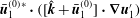 $\bar{\boldsymbol{u}}_{1}^{(0)\ast }\boldsymbol{\cdot }([\hat{\boldsymbol{k}}+\bar{\boldsymbol{u}}_{1}^{(0)}]\boldsymbol{\cdot }\unicode[STIX]{x1D735}\boldsymbol{u}_{1}^{\prime })$
, and (ii) those due to mixing of the two flow fields, e.g.
$\bar{\boldsymbol{u}}_{1}^{(0)\ast }\boldsymbol{\cdot }([\hat{\boldsymbol{k}}+\bar{\boldsymbol{u}}_{1}^{(0)}]\boldsymbol{\cdot }\unicode[STIX]{x1D735}\boldsymbol{u}_{1}^{\prime })$
, and (ii) those due to mixing of the two flow fields, e.g.
 $\bar{\boldsymbol{u}}_{1}^{(0)\ast }\boldsymbol{\cdot }([\hat{\boldsymbol{k}}+\bar{\boldsymbol{u}}_{1}^{(0)}]\boldsymbol{\cdot }\unicode[STIX]{x1D735}\boldsymbol{u}_{2}^{\prime })$
. Using the above-mentioned fluid velocity decay rates, scaling analysis then shows that this self-interaction contributes terms of
$\bar{\boldsymbol{u}}_{1}^{(0)\ast }\boldsymbol{\cdot }([\hat{\boldsymbol{k}}+\bar{\boldsymbol{u}}_{1}^{(0)}]\boldsymbol{\cdot }\unicode[STIX]{x1D735}\boldsymbol{u}_{2}^{\prime })$
. Using the above-mentioned fluid velocity decay rates, scaling analysis then shows that this self-interaction contributes terms of
 $O(1/A)$
to
$O(1/A)$
to
 $U_{prop}$
, whereas contributions from the mixed terms are of
$U_{prop}$
, whereas contributions from the mixed terms are of
 $O(1/A^{2})$
.
$O(1/A^{2})$
.
As such, the dumbbell’s two spheres are hydrodynamically isolated in the large aspect ratio limit,
 $A\gg 1$
, and (B 1) gives the required leading-order asymptotic result for the fluid’s velocity field generated by the dumbbell.
$A\gg 1$
, and (B 1) gives the required leading-order asymptotic result for the fluid’s velocity field generated by the dumbbell.


