2.1 Laboratory fatigue test of the drawbar

Laboratory fatigue test of the drawbar is carried out to examine the durability of the structure and test whether the structural fatigue life can meet the service requirements and improve the design, optimising the structure and prolonging service life.

Before structure experiments, the material basic mechanical properties are measured. Figure 1 shows the true stress-strain curve of the high-strength steel, which is obtained through variation from the nominal stress-strain relationship.

Figure 1. The true strain-stress curve of high-strength steel under tensile load.

The drawbar suffers a shocking load during taking off. Figure 2 presents the load history. It can also be illustrated that the R ratio is zero in the fatigue test.

Figure 2. Load history of the drawbar.

Then a laboratory test is carried out, the fracture is found on the head drawbar in the lab experiment, and the rest tests of the fatigue experiment are found the failure in the same region during 2,575 life repeats on average.

The crack initiates from the groove root of the drawbar, then spreads upward to form a fracture and ultimately causes a fracture failure. Through the analysis of the fracture of the drawbar, and the life repeats reveal that failure belongs to the strain fatigue category.

2.2 Laboratory test results compared with simulation

FEM analysis software HyperMesh is used to simulate the stress feedback in the process of drawbar under tensile load. The FEM model is established as shown in the picture, meshing by Tetra10, with an amount of 94,572 elements in the size of 3 mm. The load direction is along the drawbar axis. All degrees of freedom at the end of the drawbar are restrained except the degree of freedom around the axis of the hole. It can be seen from Fig. 3, all nodes degrees except Rotation-X are constrained.

Figure 3. FEM model of the drawbar.

A general implicit algorithm is utilised under statistic load conditions, Von-Mises stress contour plot (Fig. 4) shows good coincidence with the result of lab experiments drawn from the figure of comparison.

Figure 4. Stress contour plot.

A static loading test of the drawbar is carried out. As the structure and its working condition is axial-symmetry, this study takes the mean value of the symmetrical strain gauge and compares simulation with test results. Figure 5 presents the positions of strain gauges. Table 1 shows the comparison between the maximum strain results measured by strain gauge and simulation results.

The good coincidence verifies the accuracy of the FEM model. From the contour plot, it can be seen that the maximum stress is 2,379MPa, located in the same position as the fracture is, which also exceeds the material high-strength steel’s yield strength. It can be concluded that the area has stepped into the plastic zone of the structure.

Table 1 Comparison of strain values

Figure 5. Positions of strain gauges.

2.3 Fatigue life analysis of drawbar

Deductions can be made that there appears strain fatigue, inferred from the smooth fracture surface, and 2,575 life repeats in the lab tests of this drawbar. This study applies the Coffin-Manson empirical formula to assess the life of the drawbar on the level of numerical theory. Of all $\Delta \varepsilon - N$ formulas, the Coffin-Manson formula is mostly used. The expression is defined as the following:

(1) \begin{equation}{\varepsilon _{\rm{a}}} = {\varepsilon _{{\rm{ea}}}} + {\varepsilon _{{\rm{pa}}}} = \frac{{{\sigma^\prime_f} }}{E}{\left( {2N} \right)^b} + {\varepsilon^\prime_f} {\left( {2N} \right)^c}.\end{equation}

${\sigma^\prime_f} $ defines the fatigue strength coefficient, ${\varepsilon^\prime_f} $ is coefficient for fatigue ductility, b is fatigue strength exponent, and c is the exponent for fatigue ductility. This formula reveals the relations between life N and elastic strain part ${\varepsilon _{{\rm{ea}}}}$, plastic strain part ${\varepsilon _{{\rm{pa}}}}$ and the total ${\varepsilon _{\rm{a}}}$.

The Coffin-Manson formula is used in structures of short or medium life repeats. When ${R_\varepsilon } \ne - 1$, average stress should be corrected, and this model also needs correction. In this study, morrow total strain correction is introduced:

(2) \begin{equation}{\varepsilon _{\rm{a}}} = \frac{{{\sigma^\prime_f} {\rm{ - }}{\sigma _{\rm{m}}}}}{{{\sigma^\prime_f} }}\left[ {\frac{{{\sigma^\prime_f} }}{E}{{\left( {2N} \right)}^b} + {\varepsilon^\prime_f} {{\left( {2N} \right)}^c}} \right]\end{equation}

where ${\sigma _{\rm{m}}}$ is the mean stress of the structure.

This study uses the fatigue analysis software nCode with its EN-CAE Fatigue module⁽⁷⁾, and the material parameters are entered as Table 2 shows. The low-cycle fatigue performance parameters of metal materials under uniform temperature and axial constant amplitude strain control are determined according to ISO 1099-2017 Metallic Materials—Fatigue Testing—Axial Force-controlled Method.

Table 2 Material fatigue parameter

Additionally, the E-N curve and elastoplastic boundary diagram of high-strength steel are drawn, and Fig. 6 shows the strain life with elastic and plastic lines.

Based on the work above, strain fatigue theory is used to calculate life repeats of the drawbar, of which life contour plot is shown as follows.

Figure 7 shows the life (repeats) contour plot, and the lowest life repeats’ region appears at node 183,862 with 3,791 repeats. Figure 8 gives the precise location of the minimum life repeats.

Figure 6. E-N curve and elastoplastic boundary of high-strength steel.

Figure 7. Life contour plot.

Compared with lab experiments, simulation results show a precise coincidence in the fracture region and life repeats. Accordingly, the Coffin-Manson criterion is applied in subsequent analysis. Due to the conservative prediction in life calculation, results estimating from the Coffin-Manson criterion are higher than that testing in the lab.

3.1 Parameters selection

Considering the structure’s practical use, the manufacturing parameters are selected, and major structural parameters of the drawbar influencing its fatigue life and stress are illustrated as follows:

• $Beta$: cutting edge angle of slotted feed knife

• $Theta$: gradient angle of the grooved web

• ${R_1}$: cutting edge radius of groove outline

• ${R_2}$: arc radius of groove outline

• ${R_3}$: radius of groove fillet

• ${D_1}$: the distance between the axis of the drawbar body and center of groove outline cutter

• ${D_2}$: the distance between the axis of drawbar head and center of groove outline cutter

• ${D_3}$: the distance between the axis of the drawbar head and groove outline

• ${D_4}$: the distance between the axis of the drawbar head and center of groove edge

• ${D_5}$: height of groove

• ${D_6}$: the distance between the axis of the drawbar head and gradient starting point

• ${D_7}$: the distance between the axis of the drawbar head and gradient ending point

• ${D_8}$: the initial thickness of web;

Figure 9 defines the 14 parameters of the drawbar in detail.

Table 3 Range of drawbar parameters

Figure 8. The node of minimum life repeats.

Initial ranges are also proposed on the basis of the drawbar geometry structural limits. On this basis, Table 3 roughly gives the range of the drawbar parameters.

3.2 Establishment of the surrogate model

When a definite functional relationship cannot express the functional relationship between the objective function and the variables, it can be fitted by using the approximation models based on the data of sample points. And then, the optimal process can be carried out on this basis, which can significantly improve the efficiency when the variable space is large.

Surrogate model methods are based on the decomposition of $Y(x) = f(x) + \varepsilon (x)$, where the error $\varepsilon (x)$ is assumed to be identical independent distribution (normal distribution), $\varepsilon (x) \sim N(0,{\sigma ^2})$ for example. The process of creating surrogate models includes:

1. (i) Acquiring sample data given by DOE test design

2. (ii) Choosing the surrogate model type

3. (iii) Initializing the surrogate model

4. (iv) Verifying the surrogate model and the prediction effect by calculating the approximate error of the model

If the reliability is not high enough, the surrogate model needs to be updated to improve its prediction accuracy. The standard method is to add more sample data and change model parameters.

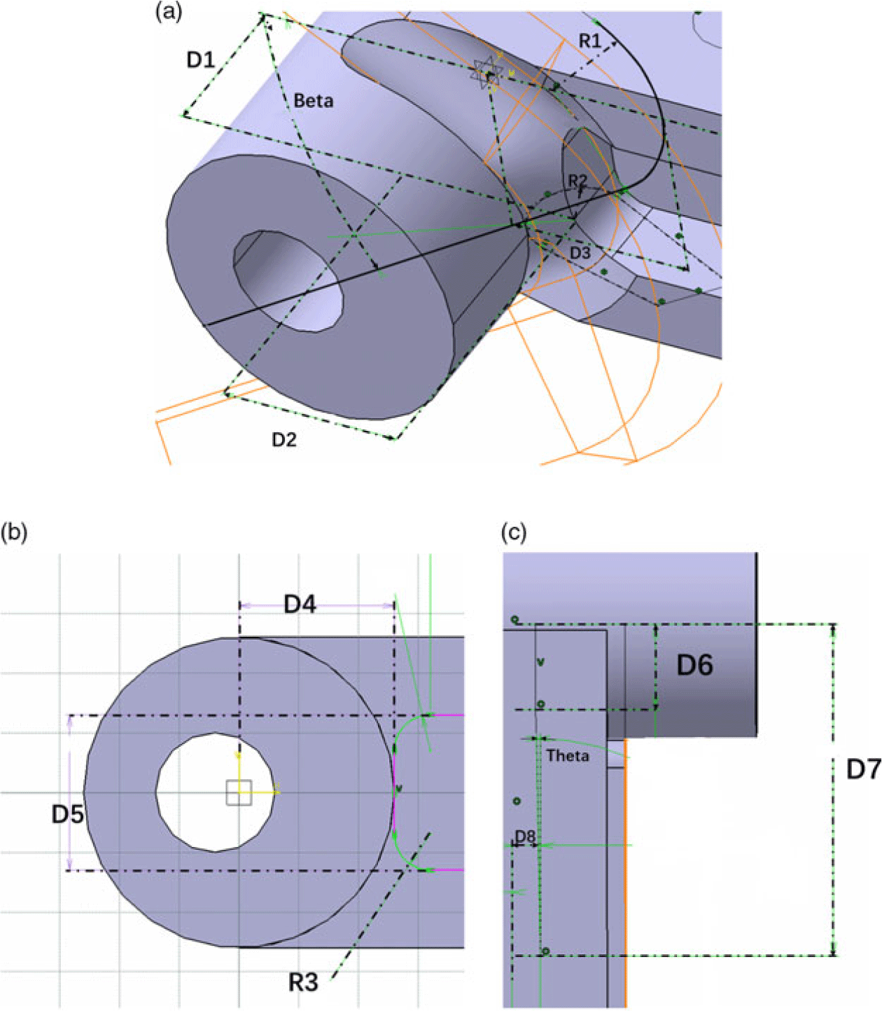
Figure 9. Major parameters of the drawbar.

If the surrogate model has enough credibility, the simulation program can be replaced by the surrogate model;

Figure 10 shows the flow chart of the surrogate model.

The commonly used surrogate models include the response surface model, neural network model, orthogonal polynomial model, and Kriging model. The radial basis function neural network model (RBF)^{(Reference Hardy8)} is chosen in this model. Its advantages lie in its strong ability to approximate complex non-linear functions in engineering applications, no need for mathematical assumptions and black box characteristics. It has a strong fault-tolerant function. Even with noisy input, a sound network overall performance can be achieved.

The classical form of the radial basis function model can be expressed as follows^{(Reference Fang and Horstemeyer9)}.

(3) \begin{equation}f(x) = \sum\limits_{i = 1}^n {{\lambda _i}} \phi \left( {\left\| {x - {x_i}} \right\|} \right)\end{equation}

where $n$ is the number of the sample points, $x$ is the design variable vector, ${x_i}$ is the vector of the design variable at the $i$th sample point, $\phi $ is a basis function, and ${\lambda _i}$ is the coefficient of the $i$th basis function. The commonly used basis functions are shown as follows.

(4) \begin{equation}{\rm{Linear\!:}}\ \ \phi (r) = r\end{equation}

(5) \begin{equation}{\rm{Gauss\!:}}\ \ \phi (r) = {e^{ - c{r^2}}},\quad (0 \lt c \lt 1)\end{equation}

(6) \begin{equation}{\rm{Multiquadric}}\!:\ \ \phi (r) = \sqrt {{r^2} + {c^2}} ,\quad (0 \lt c \lt 1)\end{equation}

R-Squard (${R^2}$) is often used to measure the degree of consistency between the surrogate model and sample points.

(7) \begin{equation}{R^2} = 1 - \frac{{\sum\limits_{i = 1}^n {({y_i} - } {{\tilde y}_i}{)^2}}}{{\sum\limits_{i = 1}^n {({y_i} - } \bar y{)^2}}}\end{equation}

where ${y_i}$, ${\tilde y_i}$, $\bar y$ represent the true values, approximate values and mean values of test point responses. The closer the value of ${R^2}$to 1, the higher the reliability of the approximation model will be. During the process, the initial number of sample points is 50; to get the best approximation content, 100 more points are added. Error analysis of the approximation model and other approximation models were also used. Figure 11 compares the ${R^2}$ values of different approximation models.

Figure 10. Process of establishing surrogate models.

As is shown above, the RBF model has the highest reliability. To comprehensively evaluate the approximation of the model, Root Mean Square Error (RMSE), Relative Average Absolute Error (RAAE) and Relative Maximum Absolute Error (RMAE) are also introduced in this study^{(Reference Jin, Chen and Simpson10)}.

(8) \begin{equation} RMSE = \sqrt {\frac{1}{n}\sum\limits_{i = 1}^n {{{\left({y_i} - {{\hat y}_i}\right)}^2}} } \end{equation}

(9) \begin{equation}\hspace*{-28pt} RAAE = \frac{{\sum\limits_{i = 1}^n {\left| {{y_i} - {{\tilde y}_i}} \right|} }}{{{n_t} \times STD}}\end{equation}

(10) \begin{equation}\hspace*{-40pt}STD = \sqrt {\frac{1}{{{n_t} - 1}}\sum\limits_{i = 1}^{{n_t}} {{y_i} - {{\tilde y}_i}} } \hspace*{30pt}\end{equation}

(11) \begin{equation}RMAE = \frac{{\max (\left| {{y_1} - {{\tilde y}_1}} \right|,\left| {{y_2} - {{\tilde y}_2}} \right|, \cdots ,\left| {{y_n} - {{\tilde y}_n}} \right|)}}{{STD}}\end{equation}

The above four equations evaluate the accuracy of the surrogate model from different perspectives, ${R^2}$, RMSE, RAAE focus on describing the overall accuracy of the model, while RMAE on the local. Table 4 shows the confidence criterion of the model, which are given by the approximation module of the ISIGHT software⁽¹¹⁾.

The previous analysis indicates that the fitting relationship between sample optimisation objectives and variables can be accurately described by using the RBF model to fit the surrogate model.

Table 4 Confidence criterion

3.3 Sensitivity analysis of drawbar parameters

Parameters affecting drawbar structure also have different influences on their static and fatigue responses, their ranges matter as well. We usually call this process sensitivity analysis. Performing sensitivity analysis can efficiently evaluate the influences of parameter varieties on structure response.

After the calculation of each sample point, the regression model is established according to the sample point. Through the Pareto chart, the relationship between each input variable and the maximum stress is analysed, as well as the information of correlation degree between variables and response. The positive effect or negative effect of each parameter on the response is also obtained. It is helpful to grasp the main parameters accurately in the design process.

Pareto chart, which is used to reflect the contribution of each input variable to each response, represents the main effect of all input variables in a given response, where blue represents the positive effect and red represents the negative effect. The value ${{\rm{N}}_{x^\prime_i}}$ is the percentage form of the model coefficient ${S_{x^\prime_i}}$ after normalising the input variable.

(12) \begin{equation}{N_{x^\prime_i}} = \frac{{{S_{x^\prime_i}}}}{{\sum\limits_j {\Big| {{S_{{x^\prime_i}}}} \Big|} }} \times 100\% \end{equation}

Figure 12 shows the Pareto chart of the analysis, and the values illustrate the positive/negative effects of each parameter. It can be illustrated from the Pareto chart that the variables ${D_4}$, ${R_3}$ have more positive effects, while the variables ${D_5}$, ${D_6}$ have more negative effects.

Figure 11. R ² values of different approximation models.

4.1 Design of experiments (DOE)

DOE is a branch of mathematical statistics and one of the most important statistical methods in product development and process optimization. Including:

• • Identifying key experimental factors

• • Determining the best combination of parameters

• • Analyzing the relationship between input and output parameters and the trend of them

• • Constructing empirical formulas and surrogate models

• • Improving the robustness of design

This study builds a DOE platform, Fig. 13 shows the platform of drawbar optimisation simulation.DOE application includes a test plan, execution test and result analysis. There exist many methods to extract sample points, such as a full factorial design, orthogonal design, central composite design, uniform design, random design, Latin hypercube design and so on.

Figure 12. Pareto chart of the 13 variables.

The Latin hypercube sampling (LHS) method is a widely used computer simulation design, which was first proposed by Mckay et al.^{(Reference Mckay12)}. It is a modified Monte Carlo method. The sample points are uniformly covered, which are more suitable for the case of more design variables. It can significantly reduce the scale of the experiment. Assuming the dimension of the design space is $d$, the number of sample points is $n$, and the range of coordinate points on a certain dimension is ${x_i} \in [{l_i},{u_i}](i = 1,2 \cdots ,d)$, ${l_i}$ represents the lower limit on this dimension, ${u_i}$ is the upper limit:

1. (1) Determining the size of sampling $n$.

2. (2) Dividing the value range of each dimension variable ${x_i}$ into n intervals, then the design space will be divided into $n_{}^d$ sub-regions.

3. (3) Randomly producing a matrix of $n \times d$, each column of which is a full random permutation, matrix X is called Latin hypercube matrix.

4. (4) Each row of matrix X corresponds to a selected small hypercube. A sample point can be obtained by randomly extracting a sample point in this region, n sample points can be obtained.

The following figure shows the distribution of sample points selected by LHS.

Compared with the original Latin hypercube method given in Fig. 14, the uniformity of the 20 sample points of $Beta$ versus ${D_1}$ in two-dimensional space obtained by the improved hypercube sample design^{(Reference Florian13)} method is obviously improved as Fig. 15 presents.

Figure 13. DOE platform of a drawbar joint simulation.

Figure 14. Distribution of sample points using LHS.

Table 5 MIGA parameters

Table 6 Optimised drawbar parameters

3.2 Optimum design of the drawbar based on MIGA

The optimisation problems in aircraft design and manufacturing engineering are often complex. The objective functions are multimodal, non-linear, discontinuous and non-differentiable. The design variables and constraint functions may also be linear, non-linear, continuous or discrete sets of variables. Traditional gradient optimization and direct search often fail to find the global optimal solution. On the basis of this cognition, global optimisation is used in this study.

Global optimisation algorithms^{(Reference Pan, Tang, Xing and Ni14)} include multi-island genetic algorithm, pointer automatic optimiser, evolutionary optimisation, adaptive simulated annealing and particle swarm optimisation.

In this paper, a multi-island genetic algorithm is used to optimise the drawbar. The parameters concerned in MIGA is listed in Table 5.

Range of the geometry is the same as those defined in DOE, and the numerical expression of the optimisation process is defined as the following:

(13) \begin{equation}\left\{ \begin{array}{l}max\quad L({X_i})\\[8pt] \textrm{s.t.}\quad {X_{il}} \le {X_i} \le {X_{iu}}\end{array} \right.\end{equation}

The parameters above are optimised and the global search is carried out to reduce the maximum stress. The final results are shown in Table 6:

The optimised results are modeled and analysed by FEM. The stress and strain contour plots are shown in Fig. 16.

Figure 15. Distribution of sample points using improved LHS.

The maximum stress value is 2,010MPa in the same position as before. Compared with 2,379MPa before optimisation, the stress level decreases by 373MPa, 15.7%. Compared with the results optimised by the multi-island genetic algorithm, the stress error is 0.74%.

Importing the stress calculation results into a fatigue analysis module for life simulation calculation, the final results are shown in Fig. 17.

Figure 16. Stress contour plot of the optimised drawbar.

Figure 17. Life contour plot after optimization.

The final fatigue life calculation results are 8,420 takeoffs and landings at node No. 653410, also with an error of 0.93% between optimisation results. Compared with that before optimisation, life repeats increase by 4,629,122%.