


1 Introduction
Sprays occur in many natural phenomena, such as sea sprays and rainfall, and also in many industrial processes and in products and applications of everyday life. Since sprays produced for the purpose of a process require the controlled atomization of a bulk liquid in a gaseous environment, strong scientific effort has been put into the investigation of atomization and sprays for a long time. Applications like spray combustion, spray drying and coating, agricultural crop spraying and medical sprays have been, and still are, extensively studied (Lefebvre & McDonell Reference Lefebvre and McDonell2017). Recent developments in nanotechnology enable the utilization of engineered nanoparticles in consumer spray products, like waterproofing sprays and body-care products such as hair sprays and deodorants, to enhance the desired effects (Kessler Reference Kessler2011). Little is known, however, about the potential for inhalation exposure and consequent health risks of such nanoparticle-laden sprays (Quadros & Marr Reference Quadros and Marr2010, Reference Quadros and Marr2011). Aiming at the assessment of health risks due to nanoparticulate contents of the sprayed liquids, the present study aims to experimentally investigate and model the flow field of pressure-atomized consumer-type sprays to gain insights into the droplet transport through the atmospheric air.
Self-similarity is a phenomenon well known in many flows and transport processes without imprinted length or time scales (Brenn Reference Brenn2017). A well-known example is the self-similar solution for the flow field of a single-phase submerged round jet by Schlichting (Reference Schlichting1933), confirmed well by experiments (Wygnanski & Fiedler Reference Wygnanski and Fiedler1969; Hussein, Capp & George Reference Hussein, Capp and George1994). Self-similar phenomena in sprays are also known from the literature. For example, Li & Shen (Reference Li and Shen1999) and Ariyapadi, Balachandar & Berruti (Reference Ariyapadi, Balachandar and Berruti2003) showed self-similar mean axial drop velocity profiles in air-assisted atomization. Alternatively, the spray was modelled as a self-similar single-phase jet with variable density, resulting in similar scaling variables as obtained for the single-phase case (Shearer, Tamura & Faeth Reference Shearer, Tamura and Faeth1979; Faeth Reference Faeth1983; Panchagnula & Sojka Reference Panchagnula and Sojka1999). Wu et al. (Reference Wu, Santavicca, Bracco and Coghe1984) investigated Diesel-type sprays and reported self-similar axial velocity profiles far downstream from the nozzle exit, where the drops and gas phase are assumed to be in dynamic equilibrium. Soltani et al. (Reference Soltani, Ghorbanian, Ashjaee and Morad2005) found self-similar regions of normalized mean drop velocities and normalized Sauter-mean diameters in sprays from liquid–liquid coaxial swirl atomizers.
In spray flames, Karpetis & Gomez (Reference Karpetis and Gomez1999) showed self-similarity of the evaporation source term. Russo & Gomez (Reference Russo and Gomez2006) showed self-similar axial velocity profiles in buoyancy-dominated laminar spray flames. Kourmatzis, Pham & Masri (Reference Kourmatzis, Pham and Masri2015) reported self-similar axial velocity profiles for the two different drop size classes  $0<d<10~\unicode[STIX]{x03BC}\text{m}$ and
  $40<d<50~\unicode[STIX]{x03BC}\text{m}$ in non-reacting sprays and turbulent spray flames in the vicinity of the nozzle exit (approximately one to ten times the nozzle diameter downstream from the orifice). Additionally, they indicate self-similar turbulence intensities deduced from the motion of the smallest drops (
 $0<d<10~\unicode[STIX]{x03BC}\text{m}$).
Based on self-similar assumptions for several characteristics of the flow field, Cossali (Reference Cossali2001) developed a one-dimensional model to predict the rate of gas entrainment into non-evaporating full-cone sprays. A recent experimental study by Dhivyaraja et al. (Reference Dhivyaraja, Gaddes, Freeman, Tadigadapa and Panchagnula2019) showed dynamic similarity of the mean drop velocities, the Sauter-mean diameters, the liquid volume fluxes and the probability density functions (PDFs) of the drop diameter in a certain cross-section (19 nozzle diameters downstream from the nozzle orifice) between sprays generated by pressure-swirl atomizers at a wide range of different flow conditions. For the theoretical description, the authors used the similarity coordinate of the single-phase jet (Schlichting Reference Schlichting1933) and modified it by introducing a constant geometrical parameter of the spray.
In many of the above discussed studies, the liquid and gas were injected simultaneously, resulting in negligible slip between the two phases. Thus, the cross-sectional averages of liquid and gas momentum flow rates remain approximately constant, endorsing self-similarity as observed for the single-phase jet (George Reference George, George and Arndt1989). In the present work we focus on the flow fields of sprays from single-fluid pressure atomization, where the motion of the gas phase is induced by momentum transfer from the liquid phase exclusively. Thus, the rate of liquid momentum transport through every spray cross-section decreases with increasing distance from the atomizer orifice, while the gas phase gains momentum.
As an atomizer type relevant for the present study, pressure atomizers with off-axis liquid supply, as in use with consumer-type spray cans, are studied. Sprays are produced at mass flow rates of the order of magnitude of many consumer sprays. Three sprays of two different liquids at different flow conditions are examined. The size and two velocity components of the drops in the spray flows are measured by phase-Doppler anemometry (PDA) in cross-sections at different distances from the atomizer orifice. In these regions of the sprays, the flow field exhibits momentum transfer from the liquid to the gas phase.
The paper is organized as follows: an overview of the experimental methods and materials used is given in § 2. The experimental results are presented in § 3. In § 4, a self-similar description of the two-phase flow velocity field is derived from boundary-layer theory, accounting for momentum transfer between the liquid and the gas phases. The paper ends with the conclusions.
2 Experimental methods and materials

Figure 1. (a) Experimental set-up and (b) PDA optics with a spray cross-section.
Table 1. Geometrical parameters and measuring ranges of the PDA system.

The aim of this study is to explore possible self-similar properties of pressure-atomized sprays. The experimental set-up is depicted in figure 1(a). The spray nozzle is mounted on a two-axis traverse system allowing for radial and axial navigation in the spray. As the measuring technique, PDA is used. A continuous-wave argon-ion laser (Coherent Innova 90C-3) serves as the light source for a two-component DANTEC PDA system. The transmitting optics focus two pairs of laser beams with the wavelengths  $488~\text{n}\text{m}$ and
  $514.5~\text{n}\text{m}$ in coinciding probe volumes (see figure 1b). The axial and radial velocity components
  $u_{l}$ and
  $v_{l}$, as well as the diameter
  $d$ of drops passing the probe volume are measured. Table 1 lists the geometrical parameters of the PDA system and the measuring ranges of the drop properties measured in the sprays. As indicated in figure 1(b), we assume the sprays to be axially symmetric. Thus, in each cross-section, the measurement points are placed on one single radial axis. We cover one half of this radial axis at a high spatial resolution, whereas we place only few measurement points on the other half of the axis to verify the assumption of axisymmetry. In order to ensure statistical reliability of the spectral spray properties, even in parts of the probability density functions where sample numbers are low, the properties of 100 000 drops were measured at each sampling point. The edge of the spray was defined at the radial positions where the frequency of drop detection was 5 % of the maximum drop detection rate in the current cross-section, or less than 300 Hz. In the PDA measurements, typical validation rates for the drop diameter between 60 % and 85 % were achieved. At measurement positions close to the nozzle exit, validation rates of 50 % occurred, since in dense spray regions the single-particle constraint of PDA is violated at a higher probability than in more dilute regions.
The sprays are produced by a single-phase pressure atomizer with off-axis liquid supply, as in use with consumer spray cans, with an orifice diameter of approximately  $D_{or}=0.4~\text{m}\text{m}$. Figure 2(a) shows a photograph of a meridional section of the atomizer, and figure 2(b) sketches the flow path of the liquid through the atomizer. Due to the off-axis feed, the liquid is ejected with angular momentum, resulting in a spray angle larger than for plain-orifice atomizers. The azimuthal component of the liquid sheet velocity induced by the off-axis feed, however, is much smaller than the axial component. Structures visualized on high-speed movies of the sheet motion showed radial motion downstream. Previous studies in the literature have shown that, even for pressure-swirl atomizers with a strong azimuthal liquid feed velocity, the swirling flow inside the atomizer is converted into radial motion within small downstream distances from the nozzle exit (Schmidt et al. Reference Schmidt, Nouar, Senecal, Rutland, Martin and Reitz1999). The corresponding azimuthal velocity component of the resulting drops is negligible against their axial and radial velocity components (Dafsari, Vashahi & Lee Reference Dafsari, Vashahi and Lee2017; Jedelsky et al. Reference Jedelsky, Maly, Pinto del Corral, Wigley, Janackova and Jicha2018). The test liquid is supplied to the atomizer from a pressurized tank at over-pressures up to 6 bar. The tank volume allows for operation times long enough for the present study, which requires the measurement of large data samples.

Figure 2. (a) Photograph of a meridional section of the atomizer and (b) the corresponding schematic sketch of the liquid flow through the atomizer.
The process of single-phase liquid atomization, with a given internal atomizer geometry and in a given gaseous environment, is governed by a characteristic liquid velocity  $\bar{u}_{or}$ through the atomizer orifice, by a length scale
  $D_{or}$ of the atomizer orifice, as well as the liquid dynamic viscosity, density and surface tension against the environment,
  $\unicode[STIX]{x1D707}_{l}$,
  $\unicode[STIX]{x1D70C}_{l}$ and
  $\unicode[STIX]{x1D70E}$, respectively. These five relevant parameters, with three basic dimensions involved, are represented by two non-dimensional groups, which may be identified as
 $$\begin{eqnarray}We=\frac{\unicode[STIX]{x1D70C}_{l}D_{or}\bar{u}_{or}^{2}}{\unicode[STIX]{x1D70E}}\quad \text{and}\quad \text{Oh}=\frac{\unicode[STIX]{x1D707}_{l}}{\sqrt{\unicode[STIX]{x1D70C}_{l}\,\unicode[STIX]{x1D70E}D_{or}}},\end{eqnarray}$$
 where the mean axial bulk velocity at the nozzle exit  $\bar{u}_{or}$ follows from the liquid volume flow rate and the cross-section of the orifice. The two non-dimensional numbers characterize the atomization process and result. Their values are used for setting the properties of the spraying processes in the experiments. In the present work, three sprays with different pairs of values of the Weber and Ohnesorge numbers are investigated. The experimental parameters, the liquid properties and the values of the resulting
  $\text{We}$ and
  $\text{Oh}$ numbers are listed in table 2. For sprays 1 and 2, water is used as the test liquid at different throughputs, resulting in equal Ohnesorge numbers, but different Weber numbers. For spray 3, an aqueous ethanol solution with an ethanol content of 10 mass per cent is used. The Ohnesorge number of spray 3 exceeds that of the two other sprays, while the mass flow rate of spray 3 is adjusted such that the Weber number is equal to the value of spray 2. The liquid throughputs are of an order of magnitude relevant for consumer sprays. All experiments were carried out at temperatures of
  $20\pm 1\,^{\circ }\text{C}$. The spray properties are measured in 10 to 13 cross-sections downstream of the nozzle orifice.

Figure 3. Instantaneous photographs of (a) spray 1, (b) spray 2 and (c) spray 3. The images were acquired with a high-speed camera at a frame rate of 10 000 frames per second, with an exposure time of  $307\,000^{-1}~\text{s}$ per frame. The white bar corresponds to a length of
  $5~\text{m}\text{m}$.
Table 2. Parameters of the experiments performed. The fluid properties are taken from Khattab et al. (Reference Khattab, Bandarkar, Fakhree and Jouyban2012) at a temperature of  $20\,^{\circ }\text{C}$.

3 Experimental results
In this section, the properties of the liquid- and the gas-phase flow fields in the sprays measured with the PDA system are presented and discussed. At the beginning, we give an overview on the atomization process of the sprays investigated.
3.1 Liquid sheet breakup and drop formation
Sprays formed by means of a pre-filming pressure atomizer are studied. Figure 3 depicts instantaneous photographs of the three sprays, illustrating the atomization process. The drop phase is formed as a result of the instability and breakup of the liquid sheet formed at the exit of the atomizer. The sheet is annular and, due to the motion relative to the ambient air, it is subject to the Kelvin–Helmholtz instability. Forces deforming and destabilizing the sheet are due to pressure and viscous stresses at the liquid–gas interface. Unstable disturbances of the sheet lead to deformations growing in time and space. Nonlinear deformations of the liquid sheet cause its local thinning and breakup into portions contracting to ligaments. The ligaments themselves are Rayleigh–Taylor and capillary unstable. They finally break up into the spray drops. Secondary breakup of the drops due to aerodynamic forces is not important in sprays like the present ones. In its motion downstream, the spray exhibits axial and radial velocity components. The spray cross-section increases and the spatial drop concentration decreases with increasing distance from the atomizer orifice. The result of the spray formation is a mixture of liquid droplets with air moving in an equilibrium state. The subject of the present study is the self-similar process of formation of that state of the spray.

Figure 4. Experimentally obtained spray characteristics. (a,c,e): number-mean drop diameter  $D_{10}$. (b,d,f): number-mean axial drop velocity
  $\bar{u}_{l}$. From top to bottom, the results of sprays 1, 2 and 3 are shown.
3.2 Liquid-phase flow field
The PDA measurement results for the liquid-phase flow field, i.e. for the droplet phase of the sprays, are presented in figure 4. As the primary results, phase-Doppler anemometry provides two velocity components and the size of the liquid droplets in the sprays. On figure 4(a,c,e), the number-mean drop diameter  $D_{10}$, and on (b,d,f), the number-mean axial drop velocity
  $\bar{u}_{l}$, are depicted for sprays 1 through 3 from top to bottom. The mean drop diameter
  $D_{10}$ is smallest at the spray axis and increases radially outwards for all the sprays. This profile shape is due to the entrainment of air into the sprays from the environment, which transports preferentially the smallest droplets towards the spray axis, thus leading to small mean drop sizes. With increasing distance from the atomizer orifice, the mean drop diameter increases along the spray axis, and the mean drop size profiles widen together with the spray flow field. The trend of the mean drop size to increase near the spray axis is due to the decrease of the number flux of the small drops, which is more pronounced for the small than for the larger drops.
The number-mean axial drop velocity profiles exhibit significant differences between the three sprays. For spray 1, with the lowest liquid mass flow rate (see table 2), a bell-shaped profile with a maximum at the spray axis can be seen very close to the nozzle exit. At the larger liquid mass flow rate of spray 2, a local velocity minimum at the spray axis and a local velocity maximum at a certain radial distance from the spray axis can be observed in the profile closest to the nozzle orifice. The difference in the near-nozzle drop velocity profiles can be explained by the state of flow and the inner geometry of the atomizer. Due to the inner geometry of the nozzle, angular momentum is imposed on the liquid flow, leading to the formation of a hollow cone-shaped liquid sheet at sufficient liquid mass flow rates. The off-axis peak in the velocity profile indicates the location of the sheet. At lower liquid mass flow rates, the angular momentum is insufficient for opening the conical sheet, leaving it rather in what is called the ‘tulip stage’ (Lefebvre & McDonell Reference Lefebvre and McDonell2017), with high velocities occurring around the spray symmetry axis. This explanation is endorsed by the obtained radial profiles of the liquid mass and momentum fluxes (not shown), which exhibit most of the liquid mass and momentum concentrated around the spray axis for spray 1, whereas for spray 2, local maxima of the liquid mass and momentum fluxes are found at the positions where the velocity profile shows its maximum. Moreover, in the obtained drop size spectra (not shown), spray 1 shows coarser atomization than spray 2, which agrees with the findings for the liquid sheet geometry, suggesting finer atomization for the fully open hollow cone than for the tulip-stage sheet. With increasing distance from the nozzle, the shapes of the velocity profiles of all three sprays evolve into one with a peak on the symmetry axis of the sprays and an additional off-axis peak. The latter is induced by the inertia-driven radial motion of large droplets. In turn, the shape of the velocity profile in the core region is mainly determined by the motion of small droplets, explaining the observed maximum at the spray axis. The profile of the number-mean axial drop velocity of spray 3 closest to the nozzle orifice is bell shaped, similar to spray 1, although the profiles of liquid mass and momentum fluxes of spray 3 (not shown) also suggest the formation of a hollow cone-shaped liquid sheet, as in spray 2. Thus, we conclude that the velocity profile closest to the nozzle exit of spray 3 represents an intermediate state, where the central and the off-axis peaks are merged into a single maximum.
3.3 Gas-phase flow field
In determining the velocity of a gas flow field in a spray flow from PDA measurements it is assumed that the smallest droplets in the spray have relaxation time scales, and therefore Stokes numbers, small enough to represent the gas flow. Thus, these small droplets act as nearly massless tracer particles in the gas flow field. The threshold droplet size to be set to ensure proper representation of the gas flow field by the droplet velocities depends on the turbulent details of the flow field, as well as on the droplet liquid density and the ambient gas dynamic viscosity. Experiments in the flow field at hand must be carried out in order to determine the threshold droplet size.

Figure 5. (a) Drop diameter–velocity correlation and (b) size class-average drop velocity as a function of the drop size at  $z=25~\text{m}\text{m}$ and
  $r=7~\text{m}\text{m}$ for spray 2.
In figure 5(a), a scatter plot of the diameter–velocity correlation (total drop velocity  $w_{l}=\sqrt{u_{l}^{2}+v_{l}^{2}}$ ) of droplets measured at a certain measurement location (
 $z=25~\text{m}\text{m}$,
  $r=7~\text{m}\text{m}$) in spray 2 is shown. The trend that the drop velocity increases with the drop size is characteristic of sprays injected into a stagnant ambient gaseous medium. In deviation from this trend, however, for the smallest droplets (approximately
  $d<20~\unicode[STIX]{x03BC}\text{m}$) a secondary cloud of data points at unexpectedly high velocities is found. Discretizing the drop size axis into size classes and determining the number-mean drop velocities
  $\bar{w}_{l}$ in each size class
  $d$, together with the variance of the velocity, yields the data in figure 5(b). According to the physical expectation, the mean velocity of the small drops indeed increases with the drop diameter. For droplets below a threshold size of, here, approximately
  $15~\unicode[STIX]{x03BC}\text{m}$, however, the trend is opposite. Since we expect the smallest droplets to decelerate fastest to the velocity of the ambient gas phase, this is an unexpected finding which requires further investigation. This effect, which we call the ‘teaspoon effect’, was reported by other authors already, but not explained (Li et al. Reference Li, Chin, Tankin, Jackson, Stutrud and Switzer1991; Li & Tankin Reference Li and Tankin1992). We are sure that this is not an artefact of the PDA measurements.

Figure 6. Bimodal velocity spectrum observed for small droplets in spray 2 at  $z=25~\text{m}\text{m}$ and
  $r=7~\text{m}\text{m}$.
Figure 6 provides a spectral view of this phenomenon. It shows the probability density function of the drop velocity  $w_{l}$ for all drops with
  $d<15~\unicode[STIX]{x03BC}\text{m}$. The data set is the same as in figure 5. The PDF exhibits two peaks, one at a relatively low velocity
  $w_{l}\approx 6~\text{m}\,\text{s}^{-1}$ and a second one at a larger velocity of
  $w_{l}\approx 25~\text{m}\,\text{s}^{-1}$. The two modes of the PDF indicate that two different physical mechanisms influence the velocity spectrum of these droplets. We attribute the first peak, at the lower drop velocity, to the mean velocity of the ambient gas flow field. It represents the drops which follow the gas flow tightly due to drag. For the second peak at the higher drop velocity, no satisfactory explanation was found yet. A detailed analysis of the PDA data revealed that these drops are systematically detected after the passage of drops approximately one order of magnitude larger in size and moving at high velocities. This may indicate a grouping effect, keeping the velocities of small drops high due to the wake of larger drops.
To determine correctly the gas velocity from bimodal velocity distributions such as the present ones, it must be ensured that the, in this sense, unphysically high droplet velocities are excluded from the data analysis. For this purpose, a threshold velocity must be determined, below which the velocities of the small droplets represent the gas velocity. For this purpose, a bimodal skewed probability density function of the form
 $$\begin{eqnarray}\left.\begin{array}{@{}c@{}}\displaystyle \unicode[STIX]{x1D6F7}(x)=q\unicode[STIX]{x1D719}_{1}(x)+(1-q)\unicode[STIX]{x1D719}_{2}(x)\quad \text{with}\\ \displaystyle \unicode[STIX]{x1D719}_{i}(x)=\frac{2}{\unicode[STIX]{x1D714}_{i}\sqrt{2\unicode[STIX]{x03C0}}}\exp \left(-\frac{(x-\unicode[STIX]{x1D709}_{i})^{2}}{2\unicode[STIX]{x1D714}_{i}^{2}}\right)\int _{-\infty }^{\hat{\unicode[STIX]{x1D6FC}}_{i}(x-\unicode[STIX]{x1D709}_{i})/\unicode[STIX]{x1D714}_{i}}\exp \left(\frac{-\unicode[STIX]{x1D70F}^{2}}{2}\right)\text{d}\unicode[STIX]{x1D70F}\end{array}\right\}\end{eqnarray}$$
 is fitted to the experimental data. Here, the weighting factor  $q$ may take values between
  $0$ and
  $1$,
$1$,  $\unicode[STIX]{x1D709}_{i}$ represents an arithmetic mean,
  $\unicode[STIX]{x1D714}_{i}^{2}$ corresponds to a variance and
  $\hat{\unicode[STIX]{x1D6FC}}_{i}$ defines the skewness of the distribution. As an example, figure 6 shows that the obtained fit curve (solid line) and the experimental data are in excellent agreement. The local minimum between the two peaks of the PDF, marked by the dashed vertical line, is defined as the threshold velocity. Thus, only drops with
  $d<15~\unicode[STIX]{x03BC}\text{m}$ and velocities smaller than the threshold velocity are taken into account for the calculation of the mean gas velocity. Using smaller drop size ranges, for example
  $d<10~\unicode[STIX]{x03BC}\text{m}$, did not change the gas velocities obtained significantly. We also point out that the bimodal velocity distributions do not occur at every measurement position in the spray. Far downstream from the atomizer, only unimodal distributions were observed, supporting the wake-based explanation of this phenomenon, since the spatial drop concentration decreases with increasing distance from the nozzle, thus reducing the interaction of drop motions in the spray.

Figure 7. Axial velocity profiles in the gas flow of the sprays deduced from the mean velocities of small droplets. (a) Spray 1, (b) spray 2.
Figure 7 shows the axial gas velocity profiles for sprays 1 and 2 deduced from the PDA measurement data using the above described method. In all cases, bell-shaped profiles are obtained. The maximum values of the velocity on the spray symmetry axis decrease with increasing distance from the atomizer. Furthermore, the rise of the local mean gas velocity at a given radial distance from the symmetry axis with increasing distance from the atomizer represents the radial expansion of the spray as it propagates in the ambient air.

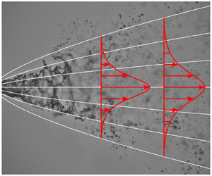
Figure 8. Self-similar flow field of an axisymmetric single-phase submerged jet.
4 Self-similar two-phase flow
In the present section, a self-similar description of the gas- and liquid-phase flow fields of pressure-atomized sprays is derived. This development constitutes a generalization of the well-known description by Schlichting (Reference Schlichting1933) for single-phase submerged free jets. The self-similar flow field of an axisymmetric single-phase jet is schematically depicted in figure 8. Its origin is a point source of mass and momentum. The axial location  $z_{0}$ of this virtual origin does not necessarily coincide with the nozzle exit (
 $z=0~\text{m}\text{m}$). Constant values of the self-similar coordinate
  $\unicode[STIX]{x1D702}$ are represented by straight lines in the
  $(r,z)$ space. Along these lines, the normalized gas velocities
  $u(r,z)/u_{0}(z)$ are constant.
4.1 Equations of motion
The flow field of the gas phase in the sprays is of turbulent boundary-layer type. Boundary-layer flows in a stagnant environment have constant pressure throughout. For the description of the turbulent shear stress in the momentum balance, the Boussinesq eddy-viscosity concept is applied. Since the turbulent eddy viscosity  $\unicode[STIX]{x1D708}_{t}$ is much greater than the molecular kinematic gas viscosity
  $\unicode[STIX]{x1D708}$, the viscous contributions to the extra stresses are neglected against the turbulent ones. The resulting axisymmetric boundary-layer equations in cylindrical coordinates for the gas phase read
 $$\begin{eqnarray}\displaystyle & \displaystyle \frac{\unicode[STIX]{x2202}u}{\unicode[STIX]{x2202}z}+\frac{1}{r}\frac{\unicode[STIX]{x2202}(vr)}{\unicode[STIX]{x2202}r}=0\quad \text{continuity gas}, & \displaystyle\end{eqnarray}$$
 $$\begin{eqnarray}\displaystyle & \displaystyle u\frac{\unicode[STIX]{x2202}u}{\unicode[STIX]{x2202}z}+v\frac{\unicode[STIX]{x2202}u}{\unicode[STIX]{x2202}r}=\unicode[STIX]{x1D708}_{t}\frac{1}{r}\frac{\unicode[STIX]{x2202}}{\unicode[STIX]{x2202}r}\left(r\frac{\unicode[STIX]{x2202}u}{\unicode[STIX]{x2202}r}\right)+f_{d}\quad z\,\text{- momentum gas}. & \displaystyle\end{eqnarray}$$
 The radial momentum balance reduces to the estimate that the dependency of pressure on the radial coordinate in the boundary-layer flow is weak. The turbulent eddy viscosity  $\unicode[STIX]{x1D708}_{t}$ is assumed to be of approximately constant value in the present case, as known from the self-similar description of turbulent single-phase jets (Tennekes & Lumley Reference Tennekes and Lumley1972; Peters Reference Peters1997). On the right-hand side of the
  $z$-momentum equation (4.2), the momentum source
  $f_{d}$ represents the transfer of momentum from the liquid to the gas phase due to the liquid injection into the gas. Heat and mass transfer between the two phases is not considered in our present analysis, i.e. the sprays are treated as non-evaporating.
The equations of motion for the liquid phase represent the constant liquid mass and the loss of momentum due to the interaction with the gas phase. For describing this process, the drops are grouped into  $N$ size classes. The liquid volume flux is determined from the PDA data as the drop volume in each size class moving in the measuring time through the Saffman-corrected probe-volume area, with account for the validation rate taken as constant for all the size classes. Denoting the liquid volume flux components of the
  $i$th drop size class in the axial and radial directions as
  $\unicode[STIX]{x1D719}_{z,i}$ and
  $\unicode[STIX]{x1D719}_{r,i}$, respectively, the continuity and
  $z$-momentum equations of the liquid phase read
 $$\begin{eqnarray}\displaystyle & \displaystyle \frac{\unicode[STIX]{x2202}}{\unicode[STIX]{x2202}z}\left(\unicode[STIX]{x1D70C}_{l}\mathop{\sum }_{i=1}^{N}\unicode[STIX]{x1D719}_{z,i}\right)+\frac{1}{r}\frac{\unicode[STIX]{x2202}}{\unicode[STIX]{x2202}r}\left(r\unicode[STIX]{x1D70C}_{l}\mathop{\sum }_{i=1}^{N}\unicode[STIX]{x1D719}_{r,i}\right)=0\quad \text{continuity liquid} & \displaystyle\end{eqnarray}$$
 $$\begin{eqnarray}\displaystyle & \displaystyle \frac{\unicode[STIX]{x2202}}{\unicode[STIX]{x2202}z}\left(\unicode[STIX]{x1D70C}_{l}\mathop{\sum }_{i=1}^{N}\bar{u}_{l,i}\unicode[STIX]{x1D719}_{z,i}\right)+\frac{1}{r}\frac{\unicode[STIX]{x2202}}{\unicode[STIX]{x2202}r}\left(r\unicode[STIX]{x1D70C}_{l}\mathop{\sum }_{i=1}^{N}\bar{u}_{l,i}\unicode[STIX]{x1D719}_{r,i}\right)=-\unicode[STIX]{x1D70C}f_{d}\quad z\,\text{- momentum liquid}. & \displaystyle\end{eqnarray}$$
 The liquid-phase continuity equation, stating that the drop mass flux is divergence free, does not account for drop coalescence and evaporation. In the  $z$-momentum balance of the liquid phase, the velocity
  $\bar{u}_{l,i}$ is the number-mean axial velocity component of the drops in size class
  $i$. Thus, the terms on the left-hand side of (4.4) represent the total axial change of momentum carried by the axial and radial liquid mass fluxes,
 $$\begin{eqnarray}\unicode[STIX]{x1D70C}_{l}\unicode[STIX]{x1D719}_{z}=\unicode[STIX]{x1D70C}_{l}\mathop{\sum }_{i=1}^{N}\unicode[STIX]{x1D719}_{z,i}\quad \text{and}\quad \unicode[STIX]{x1D70C}_{l}\unicode[STIX]{x1D719}_{r}=\unicode[STIX]{x1D70C}_{l}\mathop{\sum }_{i=1}^{N}\unicode[STIX]{x1D719}_{r,i},\end{eqnarray}$$
respectively, which is balanced by a force term on the right-hand side. Neglecting gravitation, the shown term represents the net force acting between the gas phase and the total liquid volume content, so that liquid–liquid momentum transfer due to drop collisions, breakup or coalescence need not be considered. As indicated by the negative sign, it appears as a sink term and dynamically couples the liquid to the gas-phase momentum balance (4.2).
4.2 Self-similar transformation
It is the aim of the present study to show self-similar behaviour of both the gas and the liquid phases in pressure-atomized sprays. For this purpose, the  $z$-momentum equation (4.2) of the gas phase is transformed into self-similar coordinates, representing velocity components as derivatives of the Stokesian streamfunction
  $\unicode[STIX]{x1D6F9}$, so that the continuity equation (4.1) is satisfied automatically. The streamfunction is defined through the axial and radial velocity components as
 $$\begin{eqnarray}u=\frac{1}{r}\frac{\unicode[STIX]{x2202}\unicode[STIX]{x1D6F9}}{\unicode[STIX]{x2202}r}\quad \text{and}\quad v=-\frac{1}{r}\frac{\unicode[STIX]{x2202}\unicode[STIX]{x1D6F9}}{\unicode[STIX]{x2202}z}.\end{eqnarray}$$
 In terms of the streamfunction, the  $z$-momentum equation of the gas phase reads
 $$\begin{eqnarray}\frac{1}{r}\frac{\unicode[STIX]{x2202}\unicode[STIX]{x1D6F9}}{\unicode[STIX]{x2202}r}\frac{1}{r}\frac{\unicode[STIX]{x2202}^{2}\unicode[STIX]{x1D6F9}}{\unicode[STIX]{x2202}r\unicode[STIX]{x2202}z}-\frac{1}{r}\frac{\unicode[STIX]{x2202}\unicode[STIX]{x1D6F9}}{\unicode[STIX]{x2202}z}\frac{\unicode[STIX]{x2202}}{\unicode[STIX]{x2202}r}\left(\frac{1}{r}\frac{\unicode[STIX]{x2202}\unicode[STIX]{x1D6F9}}{\unicode[STIX]{x2202}r}\right)=\unicode[STIX]{x1D708}_{t}\frac{1}{r}\frac{\unicode[STIX]{x2202}}{\unicode[STIX]{x2202}r}\left[r\frac{\unicode[STIX]{x2202}}{\unicode[STIX]{x2202}r}\left(\frac{1}{r}\frac{\unicode[STIX]{x2202}\unicode[STIX]{x1D6F9}}{\unicode[STIX]{x2202}r}\right)\right]+f_{d}.\end{eqnarray}$$
 The self-similar coordinate  $\unicode[STIX]{x1D702}$ and the streamfunction
  $\unicode[STIX]{x1D6F9}$ are assumed to take the forms
 $$\begin{eqnarray}\unicode[STIX]{x1D702}=r\,g(z),\quad \unicode[STIX]{x1D6F9}=h(z)\,f(\unicode[STIX]{x1D702}),\end{eqnarray}$$
 where  $g(z)$ is a scaling and
  $h(z)$ a mapping function. The function
  $f(\unicode[STIX]{x1D702})$ represents the self-similar shape function. Introducing (4.8) into (4.7) yields
 $$\begin{eqnarray}\left(\frac{h^{\prime }}{\unicode[STIX]{x1D708}_{t}}+\frac{2}{\unicode[STIX]{x1D708}_{t}}\frac{g^{\prime }}{g}h\right)f^{\prime \,2}-\frac{h^{\prime }}{\unicode[STIX]{x1D708}_{t}}\unicode[STIX]{x1D702}f\left(\frac{f^{\prime }}{\unicode[STIX]{x1D702}}\right)=\unicode[STIX]{x1D702}\left[\unicode[STIX]{x1D702}\left(\frac{f^{\prime }}{\unicode[STIX]{x1D702}}\right)^{\prime \,}\right]^{\prime }+\frac{1}{\unicode[STIX]{x1D708}_{t}g^{4}h}\unicode[STIX]{x1D702}^{2}f_{d},\end{eqnarray}$$
 where the prime denotes the derivative with respect to the coordinate  $\unicode[STIX]{x1D702}$ for
  $f(\unicode[STIX]{x1D702})$ and with respect to the coordinate
  $z$ for
  $g(z)$ and
  $h(z)$. The functions
  $g(z)$ and
  $h(z)$, as well as the source term
  $f_{d}$, must allow (4.9) to become an ordinary differential equation for
  $f(\unicode[STIX]{x1D702})$. This results in the requirements that
 $$\begin{eqnarray}\displaystyle & \displaystyle \frac{h^{\prime }}{\unicode[STIX]{x1D708}_{t}}=\text{constant}=:\tilde{A}, & \displaystyle\end{eqnarray}$$
 $$\begin{eqnarray}\displaystyle & \displaystyle \frac{h^{\prime }}{\unicode[STIX]{x1D708}_{t}}+\frac{2}{\unicode[STIX]{x1D708}_{t}}\frac{g^{\prime }}{g}h=\text{constant}=:\tilde{C}, & \displaystyle\end{eqnarray}$$
 so that the functions  $h(z)$ and
  $g(z)$ read
 $$\begin{eqnarray}\displaystyle & \displaystyle h(z)=\tilde{A}\unicode[STIX]{x1D708}_{t}z+\tilde{B}, & \displaystyle\end{eqnarray}$$
 $$\begin{eqnarray}\displaystyle & \displaystyle g(z)=\tilde{D}\left(\tilde{A}\unicode[STIX]{x1D708}_{t}z+\tilde{B}\right)^{(\tilde{C}-\tilde{A})/2\tilde{A}}=\tilde{D}h(z)^{(\tilde{C}-\tilde{A})/2\tilde{A}} & \displaystyle\end{eqnarray}$$
 with the four constants  $\tilde{A},\tilde{B},\tilde{C}$ and
  $\tilde{D}$. For the source term of (4.9) to be independent of the
  $z$ coordinate, we require it to be of the form
 $$\begin{eqnarray}f_{d}=\unicode[STIX]{x1D708}_{t}\tilde{A}g^{4}h\unicode[STIX]{x1D6FA}(\unicode[STIX]{x1D702}),\end{eqnarray}$$
 where  $\unicode[STIX]{x1D6FA}(\unicode[STIX]{x1D702})$ is a yet unknown self-similar shape function.
Introducing the constants
 $$\begin{eqnarray}\unicode[STIX]{x1D6FC}:=-\frac{\tilde{C}-\tilde{A}}{2\tilde{A}},\quad z_{0}:=-\frac{\tilde{B}}{\tilde{A}\unicode[STIX]{x1D708}_{t}},\quad C:=\tilde{A}\unicode[STIX]{x1D708}_{t},\quad D:=\tilde{D}(\tilde{A}\unicode[STIX]{x1D708}_{t})^{(\tilde{C}-\tilde{A})/2\tilde{A}},\end{eqnarray}$$
the ansatz for self-similarity (4.8) and for the momentum source term (4.14) become
 $$\begin{eqnarray}\unicode[STIX]{x1D702}=D\frac{r}{(z-z_{0})^{\unicode[STIX]{x1D6FC}}},\quad \unicode[STIX]{x1D6F9}=C(z-z_{0})f(\unicode[STIX]{x1D702}),\quad f_{d}=C^{2}D^{4}(z-z_{0})^{1-4\unicode[STIX]{x1D6FC}}\unicode[STIX]{x1D6FA}(\unicode[STIX]{x1D702}),\end{eqnarray}$$
 where  $z_{0}$ marks the virtual origin of the self-similar flow field,
  $\unicode[STIX]{x1D6FC}$ is an exponent and
  $C$ and
  $D$ are constants required for dimensional reasons. The self-similar transform of the
  $z$-momentum equation (4.9) reads
 $$\begin{eqnarray}(1-2\unicode[STIX]{x1D6FC})f^{\prime \,2}-\unicode[STIX]{x1D702}f\left(\frac{f^{\prime }}{\unicode[STIX]{x1D702}}\right)^{\prime }=\frac{\unicode[STIX]{x1D708}_{t}}{C}\unicode[STIX]{x1D702}\left[\unicode[STIX]{x1D702}\left(\frac{f^{\prime }}{\unicode[STIX]{x1D702}}\right)^{\prime \,}\right]^{\prime }+\unicode[STIX]{x1D702}^{2}\unicode[STIX]{x1D6FA}(\unicode[STIX]{x1D702}).\end{eqnarray}$$
 Note that, for  $\unicode[STIX]{x1D6FC}=1$ and
  $\unicode[STIX]{x1D6FA}(\unicode[STIX]{x1D702})=0$, this equation reduces to the self-similar momentum equation of the submerged single-phase round jet (Brenn Reference Brenn2017). The axial and radial velocity components (4.6) turn into
 $$\begin{eqnarray}u=CD^{2}(z-z_{0})^{1-2\unicode[STIX]{x1D6FC}}\frac{f^{\prime }}{\unicode[STIX]{x1D702}}\quad \text{and}\quad v=CD(z-z_{0})^{-\unicode[STIX]{x1D6FC}}\left(\unicode[STIX]{x1D6FC}f^{\prime }-\frac{f}{\unicode[STIX]{x1D702}}\right).\end{eqnarray}$$
The solution of (4.17) is subject to three boundary conditions for the gas flow field. The first two read
 $$\begin{eqnarray}\displaystyle & \displaystyle u|_{\unicode[STIX]{x1D702}\rightarrow 0}=\text{finite}\quad \Rightarrow \quad f^{\prime }(0)=0, & \displaystyle\end{eqnarray}$$
 $$\begin{eqnarray}\displaystyle & \displaystyle v|_{\unicode[STIX]{x1D702}\rightarrow 0}=0\quad \Rightarrow \quad f(0)=0, & \displaystyle\end{eqnarray}$$
 where we made use of the formulation of the velocity components with the self-similar function  $f(\unicode[STIX]{x1D702})$ in (4.18). The third boundary condition
  $f^{\prime \prime }(0)$ cannot be determined from general considerations on the velocity components of the flow field. Indeed, for single-phase submerged free jets, the solution of Schlichting (Reference Schlichting1933) shows that
  $f^{\prime \prime }(0)$ depends on global parameters of the flow field, such as the global momentum flow rate and the fluid properties. We expect a similar relation in the present case. In order to solve equation (4.17) for
  $f(\unicode[STIX]{x1D702})$, the quantities
  $z_{0}$,
  $\unicode[STIX]{x1D6FC}$,
  $\unicode[STIX]{x1D708}_{t}$,
  $C$,
$C$,  $D$ and
  $\unicode[STIX]{x1D6FA}(\unicode[STIX]{x1D702})$ must be determined.
4.3 Determination of the virtual origin  $z_{0}$ and the exponent $\unicode[STIX]{x1D6FC}$


The virtual origin  $z_{0}$ and the exponent
  $\unicode[STIX]{x1D6FC}$, and additional information relating to the self-similar solution, are determined from the self-similar representation (4.16) by linking the self-similar transformed flow quantities to the experimental data. For this purpose, the experimentally measured gas velocity on the symmetry axis of the spray
  $u_{0}(z)$, where
  $r=0$, i.e.
  $\unicode[STIX]{x1D702}=0$, is represented by the formulation in (4.18), which reads
 $$\begin{eqnarray}u_{0}(z)=\underbrace{CD^{2}f^{\prime \prime }(0)}_{=:U_{exp}}(z-z_{0})^{1-2\unicode[STIX]{x1D6FC}}.\end{eqnarray}$$
 Second, as required by self-similarity, the normalized gas velocities  $u/u_{0}$ have to satisfy
 $$\begin{eqnarray}\frac{u}{u_{0}}=\text{constant}\quad \text{for }\unicode[STIX]{x1D702}=D\frac{r}{(z-z_{0})^{\unicode[STIX]{x1D6FC}}}=\text{constant}.\end{eqnarray}$$
 The quantities  $z_{0}$,
  $\unicode[STIX]{x1D6FC}$,
  $U_{exp}$ and the ratios
  $\unicode[STIX]{x1D702}/D$ associated with the normalized axial gas velocities are determined by a data fit such that both conditions (4.21) and (4.22) are satisfied.
Further to the constraints (4.21) and (4.22), the self-similar solution must meet the axial dependency of the momentum flow rate  ${\mathcal{I}}(z)$ of the gas phase deduced from the experiments. In general, and in self-similar coordinates, the rate of axial momentum transport through a plane
  $z=\text{constant}$ is defined by
 $$\begin{eqnarray}{\mathcal{I}}(z)=2\unicode[STIX]{x03C0}\unicode[STIX]{x1D70C}\int _{r=0}^{\infty }u^{2}r\,\text{d}r=\underbrace{2\unicode[STIX]{x03C0}\unicode[STIX]{x1D70C}C^{2}D^{2}\int _{\unicode[STIX]{x1D702}=0}^{\infty }\frac{f^{\prime \,2}}{\unicode[STIX]{x1D702}}\,\text{d}\unicode[STIX]{x1D702}}_{=:M_{exp}}\left(z-z_{0}\right)^{2-2\unicode[STIX]{x1D6FC}}.\end{eqnarray}$$
 In contrast to the single-phase jet, the momentum transport rate of the gas phase is not constant, but it increases with the  $z$ coordinate due to momentum transfer from the liquid to the gas phase. To determine the experimental momentum transport rate of the gas phase, we require an analytical expression of the axial gas velocity
  $u$ obtained experimentally at discrete positions
  $r_{i}$ (see figure 7). For this purpose, the measured axial gas velocity profiles of each cross-section are fitted with a bell-shaped function of the form
 $$\begin{eqnarray}u(r,z)=\frac{A_{1}(z)}{\left(1+A_{2}(z)\,r^{2}\right)^{2}},\end{eqnarray}$$
 with the two independent parameters  $A_{1}(z)$ and
  $A_{2}(z)$. The obtained velocity profiles (4.24) are in excellent agreement with the experimental data, as exemplarily depicted in figure 9. With these profiles, the evolution of
  ${\mathcal{I}}(z)$ is calculated from the experiments, and the parameter
  $M_{exp}$ is determined by curve fitting.

Figure 9. Experimental and fitted axial gas velocity profiles at  $z=35~\text{m}\text{m}$ for the three sprays.
The two parameters  $U_{exp}$ and
  $M_{exp}$ in (4.21) and (4.23) relate to the self-similar function
  $f(\unicode[STIX]{x1D702})$ as per
 $$\begin{eqnarray}U_{exp}=CD^{2}f^{\prime \prime }(0)\quad \text{and}\quad M_{exp}=2\unicode[STIX]{x03C0}\unicode[STIX]{x1D70C}C^{2}D^{2}\int _{\unicode[STIX]{x1D702}=0}^{\infty }\frac{f^{\prime \,2}}{\unicode[STIX]{x1D702}}\,\text{d}\unicode[STIX]{x1D702}.\end{eqnarray}$$
 They represent equations for determining the model constants  $C$ and
  $D$. In order to determine their values, the self-similar shape function
  $f(\unicode[STIX]{x1D702})$ is required.
In table 3, the values of  $z_{0}$ and
  $\unicode[STIX]{x1D6FC}$, and of the quantities
  $U_{exp}$ and
  $M_{exp}$, determined from the experiments, are listed. Notably, the exponent
  $\unicode[STIX]{x1D6FC}$ is close to a value of
  $2/3$ for all the three sprays investigated. It differs significantly from the single-phase round jet, where its value is unity. The lower value of
  $2/3$ in the two-phase flow indicates that self-similarity coordinate lines
  $\unicode[STIX]{x1D702}=\text{constant}$ are no longer straight, as in the single-phase jet shown in figure 8, but curved, which is due to the acceleration of the gas phase by the liquid drops. As such, the more slowly diverging coordinate lines reflect the physical process of momentum transfer between the two phases. The virtual origins are located inside the nozzle, as indicated by the negative values obtained. The values of
  $U_{exp}$ and
  $M_{exp}$ increase with the Weber and Ohnesorge numbers. A larger Weber number relates to a larger injected liquid momentum flow rate, resulting in a higher gas velocity along the spray axis, i.e. in larger values of
  $U_{exp}$. Accordingly, the total rate of momentum transfer from the liquid to the gas phase is higher, as indicated by larger values of
  $M_{exp}$. At a larger Ohnesorge number, as in spray 3, the liquid atomization leads to smaller droplets (compare figures 4(c) and 4(e)). The smaller droplets with the larger total surface experience more intense momentum transport to the gas phase, resulting in larger values of
  $M_{exp}$ and
  $U_{exp}$.
Figures 10 and 11 show that the descriptions of the maximum gas velocity, the momentum flow rate and the profiles of the normalized axial gas velocity in the flow fields achieved represent the experimental data very well. In figure 10(a), the decrease of the axial gas velocity along the symmetry axes of the three sprays is depicted. Figure 10(b) shows the increase of the axial momentum flow rate of the gas phase with increasing distance from the atomizer. For all three sprays, the experimental data are matched very well by (4.21) and (4.23).

The values of the exponent  $\unicode[STIX]{x1D6FC}$ in (4.23) listed in table 3 indicate that the gas momentum flow rate increases as
  $\propto (z-z_{0})^{2/3}$. This axial increase is slower than that obtained by Cossali et al. (Reference Cossali, Gerla, Coghe and Brunello1996), who measured the gaseous mass flow rate entrained into an unsteady full-cone spray, which is defined as
 $$\begin{eqnarray}{\dot{m}}_{e}(z)=2\unicode[STIX]{x03C0}\unicode[STIX]{x1D70C}\int _{r=0}^{\infty }u(r,z)r\,\text{d}r.\end{eqnarray}$$
 Assuming the self-similar coordinate applied in single-phase jets,  $\unicode[STIX]{x1D702}_{sp}=r/(z-z_{0})$, and expressing the characteristic velocity scale in terms of the measured entrained mass flow rate
  ${\dot{m}}_{e}$, they arrive at a linear dependency of the momentum flow rate,
  ${\mathcal{I}}\propto (z-z_{0})$. This different scaling may be attributed to differences in the interaction between the liquid and the gas phases occurring in the near field of their considered unsteady full-cone diesel spray as compared to the presently investigated sprays.

Figure 10. (a) Axial gas velocity on the symmetry axis of the spray as a function of the axial position. (b) Gas momentum flow rate as a function of the axial position. The parameters used for computing the curves in both diagrams are listed in table 3.
The scaled experimental axial velocity profiles  $u/u_{0}$ in figure 11 collapse very well when plotted against the coordinate
  $\unicode[STIX]{x1D702}/D$. Minor deviations are seen for sprays 2 and 3 in the cross-sections closest to the nozzle exit (
 $z=15~\text{m}\text{m}$). In this region, the self-similar behaviour of the spray flow is not fully developed yet, which is a well-known behaviour of boundary-layer flows. Additionally, figure 12 shows the scaled radial velocity profiles
  $v(z-z_{0})^{\unicode[STIX]{x1D6FC}}$ as given by (4.18) versus the coordinate
  $\unicode[STIX]{x1D702}/D$. They collapse as well for all the three sprays. Due to the larger measurement uncertainty of the relatively small radial velocity components, the scatter is larger than for the axial gas velocity profiles.

Figure 11. Self-similar profiles of the normalized axial gas flow velocity for (a) spray 1, (b) spray 2 and (c) spray 3.

Figure 12. Self-similar profiles of the normalized radial gas flow velocity for (a) spray 1, (b) spray 2 and (c) spray 3.
4.4 Determination of the self-similar shape function $f(\unicode[STIX]{x1D702})$

The determination of the shape function  $f(\unicode[STIX]{x1D702})$ requires the coupled solution of the dynamic problem of (4.17) together with the self-similar equivalents of (4.3) and (4.4). For this purpose, a functional description of the shape function
  $\unicode[STIX]{x1D6FA}(\unicode[STIX]{x1D702})$ of the momentum source term is required, which would have to be deduced from the PDA measurement data. The determination of fluxes from PDA data, however, is inaccurate (Roisman & Tropea Reference Roisman and Tropea2001; Bade & Schick Reference Bade and Schick2011).
We therefore propose the different approach of assuming that the self-similar shape function  $f(\unicode[STIX]{x1D702})$ is of the form
 $$\begin{eqnarray}f(\unicode[STIX]{x1D702})=\frac{\unicode[STIX]{x1D702}^{2}}{1+\unicode[STIX]{x1D702}^{2}/4},\end{eqnarray}$$
which is the solution for the submerged single-phase round jet (Schlichting Reference Schlichting1933). With the help of (4.18), the self-similar profiles in figure 11 become
 $$\begin{eqnarray}\frac{u}{u_{0}}=\frac{1}{f^{\prime \prime }(0)}\frac{f^{\prime }(\unicode[STIX]{x1D702})}{\unicode[STIX]{x1D702}}=\frac{1}{\left(1+\unicode[STIX]{x1D702}^{2}/4\right)^{2}}.\end{eqnarray}$$
 Using (4.27), the constants  $C$ and
  $D$ are calculated from (4.25a,b) to
 $$\begin{eqnarray}C=\frac{3}{8\unicode[STIX]{x03C0}}\frac{M_{exp}}{\unicode[STIX]{x1D70C}U_{exp}},\quad D=2U_{exp}\sqrt{\frac{\unicode[STIX]{x03C0}}{3}\frac{\unicode[STIX]{x1D70C}}{M_{exp}}}.\end{eqnarray}$$
 With the knowledge of the constant  $D$, the scaled gas velocity profiles of all three sprays in figure 11 may be represented in a single diagram. This is shown in figure 13, where the self-similar velocity profiles of all three sprays collapse excellently on the single profile given by the self-similar function (4.28) evaluated with the solution (4.27) for
  $f(\unicode[STIX]{x1D702})$ (solid line).

Figure 13. Universal self-similar axial velocity profile of the gas flow field in the three sprays.
With the self-similar shape function  $f(\unicode[STIX]{x1D702})$ known, the shape function of the momentum source term
  $\unicode[STIX]{x1D6FA}(\unicode[STIX]{x1D702})$ from the self-similar transformed
  $z$-momentum equation (4.17) can be calculated. Before doing this, in the next section we determine the turbulent eddy viscosity
  $\unicode[STIX]{x1D708}_{t}$, which will be required to evaluate
  $\unicode[STIX]{x1D6FA}(\unicode[STIX]{x1D702})$.
4.5 Determination of the turbulent eddy viscosity $\unicode[STIX]{x1D708}_{t}$

The turbulent eddy viscosity of the gas flow field is determined from the PDA data. The analysis is based on the Boussinesq eddy-viscosity concept, representing the turbulent  $(r,z)$ shear stress as per
 $$\begin{eqnarray}-\overline{u^{\prime }v^{\prime }}=\unicode[STIX]{x1D708}_{t}\frac{\unicode[STIX]{x2202}u}{\unicode[STIX]{x2202}r}.\end{eqnarray}$$
 Here,  $u^{\prime }$ and
  $v^{\prime }$ denote the axial and radial velocity fluctuations of the gas phase, respectively. The fluctuations are a property of the gas flow field induced by the motion of the liquid phase. In sprays, the presence of droplets dampens or enhances the gas-phase turbulence through mechanisms well reported in the literature (Balachandar & Eaton Reference Balachandar and Eaton2010). In the sprays investigated in the present study, a dampening effect dominates due to the moderate drop Reynolds numbers. Only a small fraction of droplets exhibits Reynolds numbers in a range where vortex shedding occurs, which is the main mechanism for the enhancement of the carrier-phase turbulence (Hetsroni Reference Hetsroni1989; Johnson & Patel Reference Johnson and Patel1999).
The cross-correlation  $\overline{u^{\prime }v^{\prime }}$ is determined from the PDA measurement data by
 $$\begin{eqnarray}\overline{u^{\prime }v^{\prime }}=\frac{\displaystyle \mathop{\sum }_{i}\mathop{\sum }_{j}n_{ij}(u-u_{i})(v-v_{j})}{\displaystyle \mathop{\sum }_{i}\mathop{\sum }_{j}n_{ij}}.\end{eqnarray}$$
 For this purpose, only the smallest drops  $d<15~\unicode[STIX]{x03BC}\text{m}$ in the measurement data sets are accounted for, since they may be assumed to represent the gas flow field properly, also under turbulent flow conditions (see § 3.3). In (4.31),
  $n_{ij}$ represents the number of drops in the axial velocity class
  $u_{i}$ with the radial velocity
  $v_{j}$.

Figure 14. Turbulent cross-correlations  $\overline{u^{\prime }v^{\prime }}$ scaled with their axial dependency according to the self-similar approach. (a) Spray 1, (b) spray 2 and (c) spray 3.
Transforming (4.30) into self-similar coordinates, the dependency
 $$\begin{eqnarray}-\overline{u^{\prime }v^{\prime }}\propto \left(z-z_{0}\right)^{1-3\unicode[STIX]{x1D6FC}}\end{eqnarray}$$
 of the cross-correlation of the turbulent velocity fluctuations on the axial coordinate is obtained. The cross-correlations calculated from the experimental data (4.31) are scaled with their axial dependency (4.32) and plotted in figure 14 against the self-similar coordinate  $\unicode[STIX]{x1D702}$ for sprays 1, 2 and 3. The profiles collapse and match well the scaled radial gradient of the axial velocity. This confirms the earlier assumption of constant turbulent eddy viscosity. The values of the turbulent eddy viscosity
  $\unicode[STIX]{x1D708}_{t}=80\unicode[STIX]{x1D708},100\unicode[STIX]{x1D708},110\unicode[STIX]{x1D708}$ are obtained for sprays 1, 2 and 3, respectively. These values are two orders of magnitude larger than the molecular kinematic viscosity
  $\unicode[STIX]{x1D708}=0.154~\text{mm}^{2}~\text{s}^{-1}$ of air at
  $20\,^{\circ }\text{C}$, in a range reported for the single-phase jet by Tennekes & Lumley (Reference Tennekes and Lumley1972) and by Peters (Reference Peters1997).
4.6 Determination of the momentum source term
With the self-similar shape function (4.27), the shape function  $\unicode[STIX]{x1D6FA}(\unicode[STIX]{x1D702})$ of the momentum source term can be calculated from (4.17) as
 $$\begin{eqnarray}\unicode[STIX]{x1D6FA}(\unicode[STIX]{x1D702})=\frac{2}{\left(1+\unicode[STIX]{x1D702}^{2}/4\right)^{4}}\left[2\left(1-2\unicode[STIX]{x1D6FC}\right)+\unicode[STIX]{x1D702}^{2}+\frac{\unicode[STIX]{x1D708}_{t}}{C}\left(2-\unicode[STIX]{x1D702}^{2}\right)\right].\end{eqnarray}$$
To verify this shape function, the solution is compared to the measurement data. For this purpose, the axial momentum source is computed from the PDA data. Due to the inaccuracy of flux terms calculated from PDA data (Roisman & Tropea Reference Roisman and Tropea2001; Bade & Schick Reference Bade and Schick2011), however, the results obtained must be interpreted with care. The deviations are predominantly due to inaccuracies in determining the effective probe-volume cross-section in PDA measurements, which is well reported in the literature (Albrecht et al. Reference Albrecht, Damaschke, Borys and Tropea2003; Sipperley, Bade & Schick Reference Sipperley, Bade and Schick2018). Thus, we just attempt to obtain from the measurements an estimate of the shape of the momentum source term, rather than an exact functional description.
The momentum source term is determined from the divergence of the drop momentum (4.4), where the liquid momentum change in space is balanced with the drag force. Since the momentum source term  $f_{d}$ is assumed to be self-similar in (4.14), the two terms on the left-hand side of (4.4)
 $$\begin{eqnarray}\unicode[STIX]{x1D6E4}_{1}:=\frac{\unicode[STIX]{x2202}}{\unicode[STIX]{x2202}z}\left(\unicode[STIX]{x1D70C}_{l}\mathop{\sum }_{i=1}^{N}\bar{u}_{l,i}\unicode[STIX]{x1D719}_{z,i}\right)\quad \text{and}\quad \unicode[STIX]{x1D6E4}_{2}:=\frac{1}{r}\frac{\unicode[STIX]{x2202}}{\unicode[STIX]{x2202}r}\left(r\unicode[STIX]{x1D70C}_{l}\mathop{\sum }_{i=1}^{N}\bar{u}_{l,i}\unicode[STIX]{x1D719}_{r,i}\right)\end{eqnarray}$$
 must exhibit self-similarity as well. Thus, the obtained profiles for each of the two terms  $\unicode[STIX]{x1D6E4}_{1}$ and
  $\unicode[STIX]{x1D6E4}_{2}$ in every cross-section are scaled with the axial dependency of the momentum source term on
  $\left(z-z_{0}\right)^{1-4\unicode[STIX]{x1D6FC}}$, as required by the self-similar ansatz (4.16). In figure 15, the results obtained are plotted against the coordinate
  $\unicode[STIX]{x1D702}/D$ for spray 1 as an example. In view of the mentioned inaccuracies inherent to the calculation of flux terms from PDA data, and the fact that the axial and radial contributions of these flux terms to the divergence are evaluated as ratios of differences to calculate
  $\unicode[STIX]{x1D6E4}_{1}$ and
  $\unicode[STIX]{x1D6E4}_{2}$, the profiles collapse well, confirming the self-similar behaviour of the liquid phase.

Figure 15. Self-similar terms of the liquid-phase  $z$-momentum equation (4.34a,b) for spray 1. (a)
  $\unicode[STIX]{x1D6E4}_{1}$, (b)
  $\unicode[STIX]{x1D6E4}_{2}$.

Figure 16. Shape functions of the momentum source terms estimated from PDA data (dashed lines) and calculated by (4.33) (solid lines).
To calculate the shape of the source term  $f_{d}$, and, subsequently, the shape function
  $\unicode[STIX]{x1D6FA}(\unicode[STIX]{x1D702})$ as defined in (4.16), the sum of the mean profiles of the scaled terms
  $\unicode[STIX]{x1D6E4}_{1}$ and
  $\unicode[STIX]{x1D6E4}_{2}$ presented in figure 15 is calculated. In figure 16(a), the momentum source terms
  $\unicode[STIX]{x1D6FA}(\unicode[STIX]{x1D702})$ for all three sprays are plotted by dashed lines. For spray 1, a bell-shaped profile with a peak at the symmetry axis of the spray is obtained. For sprays 2 and 3, the profiles exhibit a local minimum at the spray axis and a peak further radially outwards. This agrees with the observation from the mean axial drop velocities in figure 4. Since we are interested in the shape of the momentum source term, all three experimentally determined profiles of
  $\unicode[STIX]{x1D6FA}(\unicode[STIX]{x1D702})$ were rescaled to the order of unity, using the scaling factors
  $11$,
$11$,  $10$ and
  $3$ for sprays 1, 2 and 3, respectively. This is reasonable, owing to the already noted inaccurate determination of mass and momentum fluxes from PDA data. The actually applied scaling factors are well consistent with previous studies in the literature showing that the evaluation of mass and momentum fluxes from PDA data may lead to overestimates of up to an order of magnitude (Tropea Reference Tropea2011; Bade & Schick Reference Bade and Schick2011).
The shape functions of the momentum source term from the self-similar solution (4.33) are depicted in figure 16(a) by solid lines. It can be seen that radially outwards, i.e. at large values of  $\unicode[STIX]{x1D702}$, the experimental trends are approximately captured. However, closer to the spray axis (
 $\unicode[STIX]{x1D702}=0$), the curves deviate. For sprays 2 and 3, even negative values of the momentum source term are obtained, which would indicate that momentum is transferred from the gas to the liquid phase. This is not physical for the present sprays.
We attribute this discrepancy to an underestimation of the turbulent eddy viscosity  $\unicode[STIX]{x1D708}_{t}$ by the PDA data. The values of
  $\unicode[STIX]{x1D708}_{t}$ are obtained from the cross-correlations of the velocity fluctuations of the smallest drops in the spray with
  $d<15~\unicode[STIX]{x03BC}\text{m}$, where
  $0<d<5~\unicode[STIX]{x03BC}\text{m}$ is the smallest drop size class due to statistical reasons. Because of their finite mass, drops can follow turbulent fluctuations only up to a threshold fluctuation frequency, as detailed by Chao (Reference Chao1964). Due to this effect, large turbulent structures up to a certain frequency are captured in the turbulent energy spectrum, resulting in values for
  $\overline{u^{\prime }v^{\prime }}$ and
  $\unicode[STIX]{x1D708}_{t}$ of the correct order of magnitude. However,
  $\unicode[STIX]{x1D708}_{t}$ is underestimated, since high-frequency turbulent fluctuations are missed due to the low-pass filtering effect from the drops. This assumption is supported by the comparison of relaxation time scales of the drops and the time scale of the smallest turbulent structures in the gas phase. According to the work of Chao (Reference Chao1964), drops with a diameter of
  $2.5~\unicode[STIX]{x03BC}\text{m}$ which represent the mean diameter of our smallest drop size class, follow turbulent fluctuations up to frequencies of the order of magnitude of
  $O(10^{3}~\text{Hz})$ for the fluids used in the present study. We obtain similar values when estimating the fluctuation frequency of the large-scale turbulent structures in the gas flow fields of the sprays investigated. However, the smallest high-frequency turbulent fluctuations occur in a frequency range of approximately
  $O(10^{4}~\text{Hz})$. For accurately measuring turbulent single-phase flows, much smaller droplets with diameters around
  $1~\unicode[STIX]{x03BC}\text{m}$ are needed, as in use as tracer particles in laser-Doppler measurements (Hussein et al. Reference Hussein, Capp and George1994).
An increase of the values of  $\unicode[STIX]{x1D708}_{t}$ reported in § 4.5 by 50 % brings the theoretical and experimental data for the momentum source term very close, as shown in figure 16(b). It is seen in figure 16 that the shape function of the momentum source term in (4.33) represents correctly the shapes of the momentum source for tulip-like sheets, as in spray 1, as well as for open sheets, as in sprays 2 and 3, where maxima occur off the symmetry axis.

Figure 17. Velocity ratio of the validity criterion (4.35) for the self-similar spray model for (a) spray 1, (b) spray 2 and (c) spray 3.
4.7 Scope and limitations of the model
The self-similar model for the two-phase flow field of a pressure-atomized spray presented allows for a convenient description of the flow fields of both phases. The agreement with the experimental data shows that transport processes form a self-similar two-phase flow field.
The model was built on a boundary-layer approximation of the gas flow field. Consequently, the analytical description is valid downstream from a distance from the atomizer orifice only, thus ensuring the slenderness of the flow field allowing for use of the boundary-layer form of the momentum equation. In the present case, the minimum distance from the atomizer required for the analytical solution to agree with the measurement is  $z/D_{or}\approx 38$. This distance is approximately two (spray 1) or three times (sprays 2 and 3) the breakup length of the liquid sheets shown in figure 3.
One characteristic of the self-similar solution is the dependency of the flow field properties on the axial coordinate following a power law of the form  $(z-z_{0})^{\unicode[STIX]{x1D6FD}}$. In the properties of the gas phase, the exponent
  $\unicode[STIX]{x1D6FD}$ is positive, while for the liquid-phase properties it is negative. The momentum throughput of the gas phase through every plane
  $z=\text{constant}$, however, can increase only in a region of the flow field where momentum transfer from the liquid to the gas phase persists, i.e. as long as the drop velocities are higher than the gas velocity. This fact sets limits to the validity of the self-similar description downstream, which do not emerge from the mathematical structure of the solutions themselves. The criterion limiting the validity of the self-similar model is the difference of the liquid from the gas velocity, normalized by the initial liquid velocity through the atomizer orifice,
 $$\begin{eqnarray}\frac{\hat{u} _{l}(r,z)-u(r,z)}{\bar{u}_{or}}>0,\end{eqnarray}$$
 where  $\hat{u} _{l}$ is the volume-mean axial drop velocity. As long as this ratio is positive, momentum is transferred from the liquid to the gas phase. The downstream boundary of the self-similar flow field described by the above model is located at an axial position where the velocity difference between the liquid and the gas phases has become small compared to the momentum-flux equivalent liquid velocity at the entry of the flow field. Figure 17 shows that the values obtained with this criterion are well above zero at all measurement locations in the three sprays investigated, so that the self-similar theory holds. The ratio in (4.35) decreases with increasing
  $z$ coordinate and flattens out, showing that the spray tends to evolve towards an equilibrium state between the droplet and the gas phases. From that state on, the liquid–gas two-phase mixture is characterized by a mixture density and continues moving at a mixture velocity, as described by others (Faeth Reference Faeth1983; Panchagnula & Sojka Reference Panchagnula and Sojka1999; Desantes et al. Reference Desantes, Salvador, López and De la Morena2011). Under these so-called ‘locally homogeneous flow’ (LHF) conditions, the treatment of the two-phase flow as a single fluid allows for the classical self-similar description of single-phase jets as found in Schlichting (Reference Schlichting1933). Aside from the LHF regime associated with zero relative velocity between the liquid and gas phases, the criterion (4.35) also excludes spray regimes where momentum transfer is not globally unidirectional. This is, e.g. the case in air-assisted and air-blast sprays, where momentum is transferred from a co-injected high-speed gas stream to the liquid phase.
5 Summary and conclusions
Pressure-atomized sprays produced at mass flow rates of consumer spray applications were investigated experimentally at different pairs of the Weber and Ohnesorge numbers. The air motion in the sprays is induced by the liquid ejected from the atomizer. Measurements with phase-Doppler anemometry cover the regions of the sprays with large slip velocities between the liquid and the gas phases, from close to the atomizer up to axial distances of 625 orifice diameters. The spray characterization by PDA shows the effects of different sheet geometries, producing sprays either with high liquid concentration around the symmetry axis, or with a hollow-cone profile. An approach is introduced to determine the gas velocity in the sprays from the PDA drop data, using the smallest spray droplets as tracer particles.
The experiments reveal self-similar behaviour of both the liquid and the gas phases, which was not reported in the literature before. The analytical solution for the self-similar flow field of the gas phase, derived from boundary-layer theory, is in excellent agreement with the experimental results. Notably, the obtained self-similar shape function of the gas flow field is similar to the single-phase jet. However, the scaling variables obtained differ significantly, resulting in a slower decrease of the axial gas velocity with increasing distance from the atomizer orifice, and a stronger radial expansion of the flow field than in the single-phase flow.
A limitation of the self-similar model is seen in the power-law dependency of the flow field variables on the axial coordinate, which is applicable only until the state of equilibrium between the states of motion of the two phases is reached.
Acknowledgements
Financial support from the Austrian Research Promotion Agency FFG (project no. 849876) is gratefully acknowledged. The present work is supported by SIINN ERA-NET, funded under the ERA-NET scheme of the Seventh Framework Programme of the European Commission, Research Directorate - General, Grant Agreement No. 265799.
Declaration of interests
The authors report no conflict of interest.


