


1. Introduction
Owing to its importance in a wide range of fundamental studies and industrial applications, significant effort has been made to study the shape optimisation for minimising aerodynamic drag over a bluff body (Bushnell & Moore Reference Bushnell and Moore1991; Bushnell Reference Bushnell2003). The deployment of computational fluid dynamics tools has played an important role in these optimisation problems (Thévenin & Janiga Reference Thévenin and Janiga2008). While a direct optimisation via high-fidelity computational fluid dynamics models gives reliable results, the high computational cost of each simulation, e.g. for Reynolds-averaged Navier–Stokes formulations, and the large amount of evaluations needed lead to assessments that such optimisations are still not feasible for practical engineering (Skinner & Zare-Behtash Reference Skinner and Zare-Behtash2018). When considering gradient-based optimisation, the adjoint method provides an effective way to calculate the gradients of an objective function with respect to design variables and alleviates the computational workload greatly (Jameson Reference Jameson1988; Giles & Pierce Reference Giles and Pierce2000; Economon, Palacios & Alonso Reference Economon, Palacios and Alonso2013; Kline, Economon & Alonso Reference Kline, Economon and Alonso2016; Zhou et al. Reference Zhou, Albring, Gauger, da Silva, Economon and Alonso2016), but the number of required adjoint computational fluid dynamics simulations is typically still prohibitively expensive when multiple optimisation objectives are considered (Mueller & Verstraete Reference Mueller and Verstraete2019). In gradient-free methods (e.g. genetic algorithm), the computational cost rises dramatically as the number of design variables is increased, especially when the convergence requirement is tightened (Zingg, Nemec & Pulliam Reference Zingg, Nemec and Pulliam2008). Therefore, advances in terms of surrogate-based optimisation are of central importance for both gradient-based and gradient-free optimisation methods (Queipo et al. Reference Queipo, Haftka, Shyy, Goel, Vaidyanathan and Kevin Tucker2005; Sun & Wang Reference Sun and Wang2019).
Recently, state-of-the-art deep learning methods and architectures have been successfully developed to achieve fast prediction of fluid physics. Among others, Bhatnagar et al. (Reference Bhatnagar, Afshar, Pan, Duraisamy and Kaushik2019) developed the convolutional neural network method for aerodynamics flow fields, while others studied the predictability of laminar flows (Chen, Viquerat & Hachem Reference Chen, Viquerat and Hachem2019), employed graph neural networks to predict transonic flows (de Avila Belbute-Peres, Economon & Kolter Reference de Avila Belbute-Peres, Economon and Kolter2020) or learned reductions of numerical errors in partial differential equation fluid solvers (Um et al. Reference Um, Brand, Holl, Fei and Thuerey2020). For the inference of Reynolds-averaged Navier–Stokes solutions, a U-net-based deep learning model was proposed and shown to be significantly faster than a conventional computational fluid dynamics solver (Thuerey et al. Reference Thuerey, Weissenow, Prantl and Hu2018). These promising achievements open up new possibilities of applying deep neural network (DNN)-based flow solvers in aerodynamic shape optimisation. In the present study we focus on evaluating the accuracy and performance of DNN-base surrogates in laminar flow regimes.
Modern deep learning methods are also giving new impetus to aerodynamic shape optimisation research. For example, Eismann, Bartzsch & Ermon (Reference Eismann, Bartzsch and Ermon2017) used a data-driven Bayesian approach to design optimisation and generated object shapes with an improved drag coefficient. Viquerat & Hachem (Reference Viquerat and Hachem2019) evaluated quantitative predictions such as drag forces using a VGG-like convolutional neural network. To improve the surrogate-based optimisation, Li et al. (Reference Li, Zhang, Martins and Shu2020) proposed a new sampling method for airfoils and wings based on a generative adversarial network. Renganathan, Maulik & Ahuja (Reference Renganathan, Maulik and Ahuja2020) designed a surrogate-based framework by training a DNN that was used for gradient-based and gradient-free optimisations. In these studies, the neural network is mainly trained to construct the mapping between shape parameters and aerodynamic quantities (e.g. lift and drag coefficients), but no flow-field information can be obtained from the network models. We instead demonstrate how deep learning models that were not specifically trained to infer the parameters to be minimised can be used in optimisation problems. The proposed deep learning model offers two advantages. First, the model is flexible as it predicts a full flow-field in a region of interest. Once trained, it can be used in different optimisation tasks with multiple objectives. This is of particular importance when considering problems such as compressor/turbine blade wake mixing (Michelassi et al. Reference Michelassi, Chen, Pichler and Sandberg2015). Second, as the model is differentiable, it can be seamlessly integrated with deep learning algorithms (de Avila Belbute-Peres et al. Reference de Avila Belbute-Peres, Smith, Allen, Tenenbaum and Kolter2018; Holl, Thuerey & Koltun Reference Holl, Thuerey and Koltun2020).
To understand the mechanisms underlying drag reduction and to develop optimisation algorithms, analytical and computational works have been specifically performed for Stokes flow and laminar steady flow over a body (Pironneau Reference Pironneau1973, Reference Pironneau1974; Glowinski & Pironneau Reference Glowinski and Pironneau1975, Reference Glowinski and Pironneau1976; Katamine et al. Reference Katamine, Azegami, Tsubata and Itoh2005; Kim & Kim Reference Kim and Kim2005; Kondoh, Matsumori & Kawamoto Reference Kondoh, Matsumori and Kawamoto2012). As far back as the 1970s, Pironneau (Reference Pironneau1973) analysed the minimum drag shape for a given volume in Stokes flow, and later for the Navier–Stokes equations (Pironneau Reference Pironneau1974). By using the adjoint variable approach, Kim & Kim (Reference Kim and Kim2005) investigated the minimal drag profile for a fixed cross-sectional area in two-dimensional laminar flow with Reynolds number range of  $Re=1$ to
  $40$. More recently Katamine et al. (Reference Katamine, Azegami, Tsubata and Itoh2005) studied the same problem at two Reynolds numbers,
  $Re=0.1$ and
  $Re=40$. With theoretical and numerical approaches, Glowinski & Pironneau (Reference Glowinski and Pironneau1975, Reference Glowinski and Pironneau1976) looked for the axisymmetric profile of given area and smallest drag in a uniform incompressible laminar viscous flow at Reynolds numbers between 100 and
  $10^{5}$ and obtained a drag-minimal shape with a wedge of angle
  $90^{\circ }$ at the front end and a cusp rear end from an initial slender profile. Although the laminar flow regimes are well studied, due to the separation and nonlinear nature of the fluid, it can be challenging for surrogate models to predict a drag-minimal shape as well as aerodynamic forces. Moreover, with the Reynolds number approaching zero, the flow field experiences a dramatic change from a separated vortical flow towards a creeping flow, which poses additional difficulties for the learning task. To our knowledge, no previous studies exist that target training a ‘generalised model’ that performs well in such a Reynolds number range. We investigate this topic and quantitatively assess the results in the context of deep learning surrogates.
In the present paper, we adopt an approach for U-net-based flow-field inference (Thuerey et al. Reference Thuerey, Weissenow, Prantl and Hu2018) and use the trained DNN as a flow solver in shape optimisation. In comparison with conventional surrogate models (Yondo, Andrés & Valero Reference Yondo, Andrés and Valero2018) and other optimisation work involving deep learning (Eismann et al. Reference Eismann, Bartzsch and Ermon2017; Viquerat & Hachem Reference Viquerat and Hachem2019; Li et al. Reference Li, Zhang, Martins and Shu2020; Renganathan et al. Reference Renganathan, Maulik and Ahuja2020), we make use of a generic model that infers flow solutions: in our case it produces fluid pressure and velocity as field quantities. i.e. given encoded boundary conditions and shape, the DNN surrogate produces a flow-field solution, from which the aerodynamic forces are calculated. Thus, both the flow field and aerodynamic forces can be obtained during the optimisation. As we can fully control and generate arbitrary amounts of high-quality flow samples, we can train our models in a fully supervised manner. We use the trained DNN models in shape optimisation to find the minimal drag profile in the two-dimensional steady laminar flow regime for a fixed cross-sectional area, and evaluate results with respect to shapes obtained using a full Navier–Stokes flow solver in the same optimisation framework. We specifically focus on the challenging Reynolds number range from 1 to 40. Methods based on both level set and Bézier curve are employed for shape parameterisation. The implementation utilises the automatic differentiation package of the PyTorch package (Paszke et al. Reference Paszke2019), so the gradient flow driving the evolution of shapes can be directly calculated (Kraft Reference Kraft2017). Here DNN-based surrogate models show particular promise as they allow for a seamless integration into the optimisation algorithms that are commonly used for training DNNs.
The purpose of the present work is to demonstrate the capability of deep learning techniques for robust and efficient shape optimisation, and for achieving an improved understanding of the inference of the fundamental phenomena involved in low-Reynolds-number flows. This paper is organised as follows. The mathematical formulation and numerical method are briefly presented in § 2. The neural network architecture and training procedure are described in § 3. Details of the experiments and the results are then presented in § 4 and concluding remarks in § 5.
2. Methodology
We first explain and validate our approach for computing the fluid flow environment in which shapes should be optimised. Afterwards, we describe two different shape parameterisiations, based on level-set and Bézier curve, which we employ for our optimisation results.
2.1. Numerical procedure
We consider two-dimensional incompressible steady laminar flows over profiles of given area and look for the minimal drag design. The profile is initialised with a circular cylinder and updated by utilising steepest gradient descent as optimisation algorithm. The Reynolds number  $Re_D$ in the present work is based on the diameter of the initial circular cylinder. It can be also interpreted that the the length scale is defined as the equivalent diameter for given area
  $S$ of an arbitrary shape, i.e.
  $D=2\sqrt {S/{\rm \pi} }$. In the present work,
  $D\approx 0.39424$ m is used.
To calculate the flow field around the profile at each iteration of the optimisation, two methods are employed in the present study. The first approach is a conventional steady solver of Navier–Stokes equations, i.e. simpleFoam within the open-source package OpenFOAM (from https://openfoam.org/). The second one is the deep learning model (Thuerey et al. Reference Thuerey, Weissenow, Prantl and Hu2018), which is trained with flow-field datasets generated by simpleFoam that consists of several thousand profiles at a chosen range of Reynolds numbers. More details of the architecture of the neural network, data generation, training and performance are discussed in § 3.
SimpleFoam is a steady-state solver for incompressible, turbulent flow using the semi-implicit method for pressure linked equations (known as SIMPLE) (Patankar & Spalding Reference Patankar and Spalding1983). The governing equations are numerically solved by a second-order finite-volume method (Versteeg & Malalasekera Reference Versteeg and Malalasekera2007). The unstructured mesh in the fluid domain is generated using open-source code Gmsh version 4.4.1. To properly resolve the viscous flow, the mesh resolution is refined near the wall of the profile and the minimum mesh size is set as  $\sim 6\times 10^{-3}D$, where
  $D$ is the equivalent circular diameter of the profile. The outer boundary, where the free-stream boundary condition is imposed, is set as 50 m (
 $\sim 32D$) away from the wall (denoted as OpenFOAM DOM50). The effects of domain size are assessed by performing additional simulations with domain sizes of 25 and 100 m away from the wall (denoted as OpenFOAM DOM25 and OpenFOAM DOM100, respectively). Here the drag coefficient
  $C_d$ is defined as the drag force divided by the projected length and dynamic head. As shown in figure 1, from
  $Re_D=0.1$ to
  $Re_D=40$, the total
  $C_d$ as well as the viscous
  $C_{d,v}$ and inviscid
  $C_{d,p}$ parts obtained from the three different domains almost collapse. Although small differences are observed when
  $Re_D<0.5$, the predictions in the range of interest [1, 40] are consistent and not sensitive to the domain size. The computation runs for 6000 iterations to obtain a converged state.

Figure 1. Drag coefficients from  $Re_D=0.1$ to 40. Surface integral values from OpenFOAM simulations are plotted as black curves. Results based on re-sampled points on Cartesian grids with resolutions of
  $128\times 128$,
  $256\times 256$ and
  $512\times 512$ are plotted as red, black and green circles, respectively. All data are compared with the experimental measurements of Tritton (Reference Tritton1959), which are shown as squares.
To validate the set-up, we compare our numerical results and literature data in terms of the surface pressure coefficient and wall shear. As ‘sanity checks’ for the numerical set-up, we also run SU2 (see Economon et al. Reference Economon, Palacios, Copeland, Lukaczyk and Alonso2016) with the same mesh for comparison. Figure 2(a) shows the distribution of the surface pressure coefficient  $(p_w-p_{\infty })/0.5\rho _{\infty }U_{\infty }^{2}$ at
  $Re_D=1$, 10 and 40. Here,
  $\theta$ is defined as the angle of the intersection of the horizontal line and the vector of the centre to a local surface point, so that
  $\theta =0^{\circ }$ is the stagnation point in the upwind side and
  $\theta =180^{\circ }$ that in the downwind side. Only half of the surface distribution is shown due to symmetry. The results agree well with the numerical results of Dennis & Chang (Reference Dennis and Chang1970), and the results for OpenFOAM and SU2 collapse. In figure 2(b), the results for OpenFOAM compare well with those predicted by SU2. The drag coefficients for Reynolds numbers ranging from 0.1 to 40 agree well with the experimental data of Tritton (Reference Tritton1959) in figure 1, which further supports that the current set-up and the solver produce reliable data.

Figure 2. Pressure coefficient and wall shear stress distributions. (a) Pressure coefficient distribution and (b) wall shear stress distribution.
To facilitate neural networks with convolution layers, the velocity and pressure field from OpenFOAM in the region of interest are re-sampled with a uniform Cartesian grid in a rectangular domain  $[-1, 1]^{2}$ (
 $\approx [-1.27D, 1.27D]^{2}$). A typical resolution used in the present study is
  $128\times 128$, corresponding to a grid size of
  $0.02D$. As also shown in figure 1, the effect of the resolution of re-sampling on the drag calculation has been studied. The details of the force calculation on Cartesian grids are given in § 2.2.1. Results with three different resolutions shown as coloured symbols, i.e.
  $128^{2}$,
  $256^{2}$ and
  $512^{2}$, compare favourably with the surface integral values based on the original mesh in OpenFOAM. Therefore, re-sampled fields on the
  $128\times 128$ grid are used in the deep learning framework and optimisation unless otherwise noted.
2.2. Shape parameterisation
2.2.1. Level-set method
The level-set method proposed by Osher & Sethian (Reference Osher and Sethian1988) is a technique that tracks an interface implicitly and has been widely used in fluid physics, image segmentation, computer vision as well as shape optimisation (Sethian Reference Sethian1999a; Sethian & Smereka Reference Sethian and Smereka2003; Baeza et al. Reference Baeza, Castro, Palacios and Zuazua2008). The level-set function  $\phi$ is a higher-dimensional auxiliary scalar function, the zero-level-set contour of which is the implicit representation of a time-dependent surface
  $\varGamma (t)=\{\boldsymbol {x}:\phi (\boldsymbol {x})=0\}$. Here, let
  $\mathcal {D}\in \mathcal {R}^{\mathcal{N}}$ be a reference domain,
  $\boldsymbol {x}\in \mathcal {D}$ and
  $\varOmega$ is a body created by the enclosed surface
  $\varGamma$. Specifically in the present study, the domain
  $\mathcal {D}$ is referred to the sampled Cartesian grid in the rectangular region, and
  $\mathcal {N}$ is 2 as we focus on two-dimensional problems. The level-set function
  $\phi$ is defined by a signed distance function:
 \begin{equation} \phi=\begin{cases} -d(\varGamma(t)) & \boldsymbol{x}\in \varOmega \\ 0 & \boldsymbol{x}\in\partial \varOmega\ (\text{on}\ \varGamma) \\ d(\varGamma(t)) & \boldsymbol{x} \in \mathcal{D}-\varOmega , \end{cases} \end{equation}
where  $d(\varGamma (t))$ denotes the Euclidean distance from
  $\boldsymbol {x}$ to
  $\varGamma$.
The arc length  $c$ and area
  $S$ of the body are formulated as
  $c=\int _{\mathcal {D}} \delta _\epsilon (\phi ) | \boldsymbol {\nabla } \phi | \, {\textrm {d}}s$ and
  $S=\int _{\mathcal {D}}H_{\epsilon }(-\phi )\, {\textrm {d}}s$. To make the operators differentiable, in the above, we use smoothed Heaviside and Dirac delta functions
  $H_{\epsilon }(x)={1}/({1+\textrm {e}^{-x/\epsilon }})$ and
  $\delta _{\epsilon }(x)=\partial _x({1}/({1+\textrm {e}^{-x/\epsilon }}))$, respectively. Here
  $\epsilon$ is a small positive number and chosen as twice the grid size (Zahedi & Tornberg Reference Zahedi and Tornberg2010). Then, the aerodynamic forces due to pressure distribution and viscous effect are described as
 $$\begin{gather} \boldsymbol{F}_{pressure}=\int_{\partial \varOmega} ( p \boldsymbol{n})\, {\textrm{d}}l = \int_{\mathcal{D}} (p\boldsymbol{n})\delta_\epsilon (\phi) | \boldsymbol{\nabla} \phi | \, {\textrm{d}}s, \end{gather}$$
 $$\begin{gather}\boldsymbol{F}_{viscous}=\int_{\partial \varOmega} ( \mu \boldsymbol{n}\times\boldsymbol{\omega}) \, {\textrm{d}}l=\int_{\mathcal{D}} (\mu \boldsymbol{n}\times\boldsymbol{\omega})\delta_\epsilon (\phi) | \boldsymbol{\nabla} \phi | \, {\textrm{d}}s. \end{gather}$$
Here,  $\boldsymbol {n}$ is the unit normal vector,
  $\boldsymbol {n}={\boldsymbol {\nabla } \phi }/{| \boldsymbol {\nabla } \phi | }$,
  $p$ is the pressure,
  $\mu$ is the dynamic viscosity and
  $\boldsymbol {\omega }=\boldsymbol {\nabla }\times \boldsymbol {v}$ is the vorticity with
  $\boldsymbol {v}$ being the velocity. A nearest-neighbour method is used to extrapolate values of pressure and vorticity inside the shape
  $\varOmega$. Then, the drag force is considered as the loss in the optimisation, i.e.
 \begin{equation} \mathcal{L}=\boldsymbol{F}_{pressure}\boldsymbol{\cdot} \hat{\boldsymbol{i}}_x+\boldsymbol{F}_{viscous}\boldsymbol{\cdot} \hat{\boldsymbol{i}}_x, \end{equation}
where  $\hat {\boldsymbol {i}}_x$ is the unit vector in the direction of the
  $x$ axis.
The minimisation of (2.4) is solved by the following equation:
 \begin{equation} \frac{\partial \phi} {\partial \tau} + V_n | \boldsymbol{\nabla} \phi | =0. \end{equation}
Here, the normal velocity is defined as  $V_n={\partial \mathcal {L}}/{\partial \phi }$. At every iteration, the Eikonal equation is solved numerically with the fast marching method to ensure
  $| \boldsymbol {\nabla } \phi | \approx 1.0$ (Sethian Reference Sethian1999b). Then, we have
  ${\partial \phi }/{\partial \tau } \propto -{\partial \mathcal {L}}/{\partial \phi }$, which is a gradient flow that minimises the loss function
  $\mathcal {L}$ and drives the evolution of the profile (He, Kao & Osher Reference He, Kao and Osher2007). For a more rigorous mathematical analysis we refer to Kraft (Reference Kraft2017). In the present work, the automatic differentiation functionality of PyTorch is utilised to efficiently minimise (2.4) via gradient descent. Note that the level-set-based surface representation and optimisation algorithm are relatively independent modules, and can be coupled with any flow solver, such as OpenFOAM and SU2, so long as the solver provides a re-sampled flow field on the Cartesian grid (e.g.
  $128\times 128$) at an iteration in the optimisation. We will leverage this flexibility by replacing the numerical solver with a surrogate model represented by a trained neural network below.
2.2.2. Bézier-curve-based parameterisation
Bézier-curve-based parametric shape parameterisation is a widely accepted technique in aerodynamic studies (Gardner & Selig Reference Gardner and Selig2003; Yang et al. Reference Yang, Yue, Li and Yang2018; Zhang et al. Reference Zhang, Qiang, Teng and Yu2020). This work utilises two Bézier curves, representing upper and lower surfaces of the profile denoted with superscript  $k=\{u,l\}$. Control points
  $\boldsymbol {P}_{i}^{k} \in \mathcal {D}$ are the parameters of the optimisation framework. The Bézier curves are defined via the following equation:
 \begin{equation} \boldsymbol{B}^{k}(t)=\sum_{i=0}^{n} \left(\begin{array}{c} n \\ i \end{array}\right) t^{i} (1-t)^{n-i} \boldsymbol{P}_{i}^{k}, \end{equation}
where  $t \in [0,1]$ denotes the sample points along the curves. The first and last control points of each curve share the same parameters to construct the closure
  $\varOmega$ of the profile.
A binary labelling of the Cartesian grid  $\mathcal {D}$ is performed as
 \begin{equation} \chi=\begin{cases} 1 & \boldsymbol{x}\in \varOmega \\ 0 & \boldsymbol{x} \in \mathcal{D}-\varOmega , \end{cases} \end{equation}
where  $\chi$ is the binary mask of the profile and
  $\boldsymbol {x}$ is the coordinate of a point on the Cartesian grid. The normal vector
  $\boldsymbol {n}$ is obtained via applying a convolution with a
  $3\times 3$ Sobel operator kernel on
  $\chi$. Then, forces are calculated as
 $$\begin{gather} \boldsymbol{F}_{pressure}= \sum_{i \in \mathcal{D}-\mathcal{\varOmega}} (p\boldsymbol{n})_i {\rm \Delta} l_i, \end{gather}$$
 $$\begin{gather}\boldsymbol{F}_{viscous}=\sum_{i \in \mathcal{D}-\mathcal{\varOmega}} (\mu\boldsymbol{n}\times\boldsymbol{\omega})_i {\rm \Delta} l_i, \end{gather}$$
where  $i$ is the index of a point outside the profile and
  ${\rm \Delta} l_i$ is the grid size at the point
  $i$. Thereby, drag
  $\mathcal {L}$ is calculated using (2.4). As for the level set representation, the shape gradient
  ${\partial \mathcal {L}}/{\partial \boldsymbol {P}_{i}^{k}}$ is computed via automatic differentiation in order to drive the shape evolution to minimise
  $\mathcal {L}$.
3. Neural network architecture and training procedure
3.1. Architecture
The neural network model is based on a U-net architecture (Ronneberger, Fischer & Brox Reference Ronneberger, Fischer and Brox2015), a convolutional network originally used for the fast and precise segmentation of images. Following the methodology of previous work (Thuerey et al. Reference Thuerey, Weissenow, Prantl and Hu2018), we consider the inflow boundary conditions (i.e.  $u_{\infty }$,
  $v_{\infty }$) and the shape of profiles (i.e. the binary mask) on the
  $128\times 128$ Cartesian grid as three input channels. In the encoding part, 7 convolutional blocks are used to transform the input (i.e.
  $128^{2}\times 3$) into a single data point with 512 features. The decoder part of the network is designed symmetrically with another 7 layers in order to reconstruct the outputs with the desired dimension, i.e.
  $128^{2}\times 3$, corresponding to the flow-field variables
  $[p, u, v]$ on the
  $128\times 128$ Cartesian grid. Leaky ReLU activation functions with a slope of 0.2 are used in the encoding layers, and regular ReLU activations in the decoding layers.
In order to assess the performance of the deep learning models, we have tested three different models with varying weight counts of 122 000,  $1.9 \times 10^{6}$ and
  $30.9 \times 10^{6}$, respectively, which are later referred to as small-, medium- and large-scale networks.
3.2. Dataset generation
For the training dataset, it is important to have a comprehensive coverage of the space of targeted solutions. In the present study, we utilise the parametric Bézier curve defined by (2.6) to generate randomised symmetric shape profiles subject to a fixed area constraint  $S$.
$S$.
To parameterise the upper surface of the profile, two points at the leading and trailing edges are fixed and four control points are positioned in different regions. As depicted in figure 3(a), the region of interest is divided into four columns separated by the border lines, and each control point of the upper Bézier curve is only allowed to be located within its corresponding column-wise region. Each column-wise region is further split into five subregions to produce diversified profiles. The subregions give  $5^{4}=625$ possible permutations, with control points being placed randomly in each subregion. This procedure is repeated for four times, in total producing
  $4 \times 625=2500$ Bézier curves. Figure 3(b) shows some examples from this set.

Figure 3. Shape generation using two Bézier curves. The region of interest is divided into four columns, and each column-wise region is further split into five subregions. (a) Bézier control points and (b) randomly generated shapes.
Based on these 2500 geometries, we then generate three sets of training data, as summarised in table 1.
(1) We run OpenFOAM with fixed
 $Re_D=1$ for all of the 2500 profiles to obtain 2500 flow fields, denoted as Dataset-1.
(2) The second dataset is similar but all of the 2500 simulations are conducted at
$Re_D=40$ (Dataset-40).(3) The third dataset is generated to cover a continuous range of Reynolds numbers, in order to capture a space of solutions that not only varies over the immersed shapes, but additionally captures dimensions of varying flow physics with respect to a chosen Reynolds number. For this, we run a simulation by randomly choosing a profile
$\varOmega ^{*}_i$ among 2500 geometries and a Reynolds number in the range $Re^{*}_D \in [0.5, 42.5]$. As we know that drag scales logarithmically with respect to Reynolds number, we similarly employ a logarithmic sampling for the Reynolds number dimension. We use a uniform distribution random variable $\kappa \in [\log {0.5}, \log {42.5}]$, leading to a $Re^{*}_D=10^{\kappa }$ uniformly distributed in log scale. In total we have obtained 8640 flow fields, which we refer to as Dataset-Range. With this size of the training dataset, the model performance converges to a stable prediction accuracy for training and validation losses, as shown in the Appendix.


Table 1. Three datasets for training the neural network models.

Shown in figure 4 is the distribution of all the flow-field samples from Dateset-Range on the  $\varOmega ^{*}_i$–
 $Re^{*}_D$ map, with
  $Re^{*}_D$ in log scale. It is worth noting that there are 2053 flow-field samples in the range
  $Re^{*}_D \in [0.5, 1.5]$ which are shown in red, 819 samples with
  $Re^{*}_D \in [8,12]$ shown in green and 195 samples with
  $Re^{*}_D \in [38, 42]$ shown in blue.

Figure 4. Distribution of flow-field samples from Dataset-Range on the  $\varOmega ^{*}_i$–
 $Re^{*}_D$ map. The indices of geometries
  $\varOmega ^{*}_i$ are from 0 to 2499. The red symbols denote the flow-field samples with
  $Re^{*}_D \in [0.5, 1.5]$, the green ones with
  $Re^{*}_D \in [8,12]$ and the blue ones with
  $Re^{*}_D \in [38, 42]$.
3.3. Preprocessing
Proper preprocessing of the data is crucial for obtaining a high inference accuracy from the trained neural networks. Firstly, the non-dimensional flow-field variables are calculated using
 \begin{equation} \left. \begin{array}{c@{}} \hat{p}_i=(p_i-p_{i, mean})/U_{\infty, i}^{2}, \\ \hat{u}_i=u_i/U_{\infty, i}, \\ \hat{v}_i=v_i/U_{\infty, i}. \end{array} \right\} \end{equation}
Here,  $i$ denotes the
  $i$th flow-field sample in the dataset,
  $p_{mean}$ the simple arithmetic mean pressure and
  $U_{\infty }=\sqrt {u_{\infty }^{2}+v_{\infty }^{2}}$ the magnitude of the free-stream velocity.
As the second step, all input channels and target flow-field data in the training dataset are normalised to the range  $[-1, 1]$ in order to minimise the errors from limited precision in the training phase. To do so, we need to find the maximum absolute values for each flow variable in the entire training dataset, i.e.
  $|\hat {p}|_{max}$,
  $|\hat {u}|_{max}$ and
  $|\hat {v}_{max}|$. Similarly, the maximum absolute values of the free-stream velocity components are
  $|u_{\infty }|_{max}$ and
  $|v_{\infty }|_{max}$. Then we get the final normalised flow-field variables in the following form:
 \begin{equation} \left. \begin{array}{c@{}} {\tilde p}_i= \hat{p}_i/|\hat{p}|_{max},\\ {\tilde u}_i= \hat{u}_i/|\hat{u}|_{max},\\ {\tilde v}_i= \hat{v}_i/|\hat{v}|_{max}, \end{array}\right\} \end{equation}
and the normalised free-stream velocities used for input channels are
 \begin{equation} \left. \begin{array}{c@{}} {\tilde u}_i= u_i/\max(|u_{\infty}|_{max}, 1\times 10^{{-}18}),\\ {\tilde v}_i= v_i/\max(|v_{\infty}|_{max}, 1\times 10^{{-}18}). \end{array}\right\} \end{equation}
The free-stream velocities appear in the boundary conditions, on which the solution globally depends, and should be readily available spatially and throughout the different layers. Thus, free-stream conditions and the shape of the profile are encoded in a  $128^{2}\times 3$ grid of values. The magnitude of the free-stream velocity is chosen such that it leads to a desired Reynolds number.
3.4. Training details
The neural network is trained with the Adam optimiser in PyTorch (Kingma & Ba Reference Kingma and Ba2014). A difference  $L_1=| \boldsymbol {y}_{truth}-\boldsymbol {y}_{prediction}|$ is used for the loss calculation. For most of the cases, the training runs converge after 100 000 iterations with a learning rate
  $6\times 10^{-4}$ and a batch size of 10 (unless otherwise mentioned). An 80 % to 20 % split is used for training and validation sets, respectively. The validation set allows for an unbiased evaluation of the quality of the trained model during training, for example, to detect overfitting. In addition, as learning rate decay is used, the variance of the learning iterations gradually decreases, which lets the training process fine-tune the final state of the model.
Figure 5 shows the training and validation losses for three models that are trained using Dataset-1, i.e. small-scale, medium-scale and large-scale models. All three models converge at stable levels of training and validation loss after 500 epochs. Looking at the training evolution for the small-scale model in figure 5(a), numerical oscillation can be seen in the early stage of the validation loss history, which is most likely caused by the smaller number of free parameters in the small-scale network. In contrast, the medium- and large-scale models show a smoother loss evolution, and the gap between validation and training losses indicates a slight overfitting as shown in figures 5(b) and 5(c). Although the training of the large-scale model exhibits a spike in the loss value at an early stage due to an instantaneous pathological configuration of mini-batch data and learned state, the network recovers, and eventually converges to lower loss values. Similar spikes can be seen in some of the other training runs, and could potentially be removed via gradient-clipping algorithms, which, however, we did not find necessary to achieve reliable convergence.

Figure 5. Training (in blue) and validation (in orange) losses of three different scales of models trained with Dataset-1. (a) Small-scale neural network, (b) medium-scale neural network and (c) large-scale neural network.
Figure 6 presents the training and validation losses for the three models trained with Dataset-40. Similarly, convergence can be achieved after 500 epochs. Compared with the training evolution at  $Re_D=1$, the models for
  $Re_D=40$ have smaller gaps between training and validation losses, indicating that the overfitting is less pronounced than for
  $Re_D=1$. We believe this is caused by the smoother and more diffusive flow fields at
  $Re_D=1$ (close to Stokes flow), in contrast to the additional complexity of the solutions at
  $Re_D=40$, which already exhibit separation bubbles.

Figure 6. Training (in blue) and validation (in orange) losses of three different scales of models trained with Dataset-40. (a) Small-scale neural network, (b) medium-scale neural network and (c) large-scale neural network.
We use Dataset-Range to train the model for a continuous range of Reynolds numbers. As this task is particularly challenging, we directly focus on the large-scale network that has  $30.9 \times 10^{6}$ weights. To achieve better convergence for this case, we run 800 000 iterations with a batch size of 5, which leads to more than 485 epochs. As shown in figure 7, training and validation losses converge to stable levels, and do not exhibit overfitting over the course of the training iterations. The final loss values are
  $1.01\times 10^{-3}$ and
  $1.31\times 10^{-3}$, respectively.

Figure 7. Training (in blue) and validation (in orange) losses of large-scale model trained with Dataset-Range.
To summarise, having conducted the above-mentioned training, we obtain seven neural network models, i.e. models of three network sizes each for Dataset-1 and Dataset-40 and a ranged model trained with Dataset-Range, as listed in table 1. These neural networks are used as surrogate models in the optimisation in the next section. We also compare the results from neural network models with corresponding optimisations conducted with the OpenFOAM solver, and evaluate the performance and accuracy of the optimisation runs.
4. Shape optimisation results
The initial shape for the optimisation is a circular cylinder with a diameter  $D\approx 0.39424$ m. The integral value of the drag force using (2.4) is adopted as the objective function. The mathematical formula of the optimisation for the shape
  $\varOmega$ bounded by curve
  $\varGamma$, the surface of the profile, is expressed as
 \begin{equation} \left. \begin{array}{c@{}} \min\ Drag({\varOmega})\\ \text{subject to area}\ S(\varOmega)=S_0 \\ \displaystyle \text{barycentre}\ \boldsymbol{b}(\varOmega) = \dfrac{1}{S(\varOmega)}\int_{\varOmega} \boldsymbol{x}\, {\textrm{d}}s = (0,0). \end{array}\right\} \end{equation}
 For the level-set representation, the profile  $\varOmega$ is the region where
  $\phi \leq 0$ and the constrained optimisation problem is solved as follows:
(1) Initialise level-set function
$\phi$ such that the initial shape (i.e. a circular cylinder) corresponds to $\phi =0$.(2) For a given
$\phi$, calculate drag (i.e. loss $\mathcal {L}$) using (2.2)–(2.4). Terminate if the optimisation converges, e.g. drag history reaches a statistically steady state.(3) Calculate the gradient
${\partial \mathcal {L}}/{\partial \phi }$. Consider an unconstrained minimisation problem and solve (2.5) as follows:
(4.2)\begin{equation} \phi^{n+1}\Longleftarrow\phi^{n} - {\rm \Delta} \tau \frac{\partial \mathcal{L}}{\partial \phi} | \boldsymbol{\nabla} \phi |. \end{equation}In practice, we update
$\phi$ using the second-order Runge–Kutta method, and discretise the convection term with a first-order upwind scheme (Sethian & Smereka Reference Sethian and Smereka2003). We assume derivatives of the flow-field variables (i.e. pressure and velocity) are significantly smaller than those with respect to the shape. Hence, we treat both fields as constants for each step of the shape evolution. To ensure the correct search direction for optimisation, we use a relatively small pseudo time step ${\rm \Delta} \tau$, which is calculated with a Courant number of 0.8.(4) To ensure
$| \boldsymbol {\nabla } \phi | \approx 1$, a fast marching method is used to solve the Eikonal equation (Sethian Reference Sethian1999b).(5) The area of the shape
$\varOmega$ is obtained by $S=\int _{\mathcal {D}}H_{\epsilon }(-(\phi +\eta ))\, {\textrm {d}}s$, where $\eta$ is an adjustable constant. We optimise $\eta$ such that $| S-S_0| <\epsilon$. Then, we update ${\phi }^{n+1} \Longleftarrow {\phi }^{n+1} + \eta$.(6) Check if the barycentre is at the origin:
$| \boldsymbol {b} - \boldsymbol {o}| <\epsilon$. If not, solve (2.5) to update $\phi ^{n+1}$ by replacing $V_n$ with a translating constant velocity so that the barycentre of the shape $\varOmega$ moves towards the origin. Continue with step (2).


While our main focus lies on level-set representations, the Bézier curve parameterisation with reduced degrees of freedom is used for comparison purposes. This highlights how differences in the shape parameterisation can influence the optimisation results. Thus, we include the Bezier parameterisation with very few control points and the level-set representation with a dense grid sampling as two extremes of the spectrum of shape representations. When Bézier curves are used, the constrained optimisation differs from the above-mentioned loop in the following way. In (1)–(3), the coordinates of Bézier curve control points are used as the design variables to be initialised and updated. In (5) and (6), the area of  $\varOmega$ and barycentre are calculated based on the region enclosed by the Bézier curve, where the binary mask of inner region is 1 and of outer region is 0.
In the optimisation experiments, the flow-field solvers used are OpenFOAM (as baseline) and small-, medium- and large-scale neural network models. As additional validation for the optimisation procedure, we also compare with additional runs based on the Bézier curve parameterisation with a large-scale neural network model. If the flow solver is OpenFOAM, Gmsh is automatically called to generate an unstructured mesh based on the curve  $\phi =0$ at every iteration. To update
  $\phi$ and calculate drag in step (2), as mentioned in §2.1, the flow-field variables are re-sampled on the
  $128\times 128$ Cartesian grid.
4.1. Optimisation experiment at $Re_D=1$

Figure 8 presents the drag coefficients over 200 optimisation iterations using OpenFOAM solver and the three neural network models. Here, the drag coefficient  $C_d$ is defined as drag divided by the projected length of the initial cylinder and dynamic head. The same definition is used for all other experiments in the present paper. As the ground truth, figure 8(a) shows the case which uses the OpenFOAM solver in the optimisation. The history of drag values, shown in blue, is calculated based on the re-sampled data on the Cartesian grid (i.e.
  $128^{2}$). For comparison, the drag values obtained from the surface integral in the OpenFOAM native postprocessing code are shown with red markers. As can be seen in figure 8(a), after convergence of the optimisation, the total drag drops 6.3 % from 10.43 to 9.78. To further break it down, the inviscid part decreases significantly from 5.20 to 2.50 (
 $\sim 51.8\,\%$) while the viscous part gradually increases from 5.23 to 7.27 (
 $\sim 31.0\,\%$). This is associated with the elongation of the shape from a circular cylinder to an ‘oval’, eventually becoming a rugby-ball shape as shown in figure 9(b).

Figure 8. Optimisation histories at  $Re_D=1$. The black solid lines denote the results using neural network models trained with Dataset-1 and the blue solid lines denote the results from OpenFOAM. Results calculated with the re-sampled flow fields on the
  $128\times 128$ Cartesian grid are denoted by
  $128^{2}$. The red cross symbols represent the OpenFOAM results obtained with its native postprocessing tool. (a) OpenFOAM, (b) small-scale neural network, (c) medium-scale neural network and (d) large-scale neural network.

Figure 9. The converged shapes at  $Re_D=1$ (a) and the intermediate states at every 10th iteration predicted by the large-scale neural network (NN) model (b).
From figures 8(b) and 8(c), one can observe the histories of the drag values are reasonably well predicted by the neural network models and agree with the OpenFOAM solution in figure 8(a). Despite the small-scale model exhibiting noticeable oscillations in the optimisation procedure, the medium- and large-scale neural network models provide smoother predictions, and the drag of both initial and final shapes agrees well with that from re-sampled data (blue lines) and that from the OpenFOAM native postprocessing code (red symbols).
Figure 9(a) depicts the converged shapes of all four solvers. The ground truth result using OpenFOAM ends up with a rugby-ball shape which achieves a good agreement with the data of Kim & Kim (Reference Kim and Kim2005). The medium- and large-scale neural network models collapse and compare favourably with the ground truth result. In contrast, the small-scale neural network model's prediction is slightly off, which is not surprising as one can observe oscillation and offset of the drag history in figure 8(b) as discussed before. A possible reason is that the small-scale model has fewer weights so that the complexity of the flow evolution cannot be fully captured. It is worth noting that the reduced performance of the Bézier representation in the present work is partly due to the discretisation errors when calculating the normal vectors in combination with a reduced number of degrees of freedom.
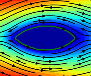
The  $x$-component velocity fields with streamlines for the optimised shapes are shown in figure 10. The flow fields and the patterns of streamlines in all three cases with neural networks show no separation, which is consistent with the ground truth result in figure 10(a). Considering the final shape obtained using the three neural network surrogates, the medium- and large-scale models give satisfactory results that are close to the OpenFOAM result.

Figure 10. Streamlines and the  $x$-component velocity fields
  $u/U_{\infty }$ at
  $Re_D=1$. (a) OpenFOAM, (b) small-scale neural network, (c) medium-scale neural network and (d) large-scale neural network.
4.2. Optimisation experiment at $Re_D=40$

As the Reynolds number increases past the critical Reynolds number  $Re_D\approx 47$, the circular cylinder flow configuration loses its symmetry and becomes unstable, which is known as the Karman vortex street. We consider optimisations for the flow regime at
  $Re_D=40$ which is of particular interest because it exhibits a steady-state solution, yet is close to the critical Reynolds number. The steady separation bubbles behind the profile further compound the learning task and the optimisation, making it a good test case for the proposed method.
The ground truth optimisation result using OpenFOAM is shown in figure 11(a). The shape is initialised with a circular cylinder and is optimised to minimise drag over 200 iterations. As a result, the total drag, processed on the Cartesian grid, drops from 1.470 to 1.269 ( $\sim$13.7 % reduction). Associated with the elongation of the shape, the inviscid drag decreases
  $41.3\,\%$ while the viscous drag increases
  $41.3\,\%$. The initial and the final results of the OpenFOAM native postprocessing are shown in red, indicating good agreement. Figure 11(b–d) presents the drag histories over 200 optimisation iterations with three neural network models that are trained with Dataset-40. Although larger oscillations are found in the drag history of the small-scale model, the medium- and large-scale models predict smoother drag history and compare well with the ground truth data using OpenFOAM.

Figure 11. Optimisation histories at  $Re_D=40$. The black solid lines denote the results using neural network models trained with Dataset-40 and the blue solid lines denote the results from OpenFOAM. Results calculated with the re-sampled flow fields on the
  $128\times 128$ Cartesian grid are denoted by
  $128^{2}$. The red cross symbols represent the OpenFOAM results obtained with its native postprocessing tool. (a) OpenFOAM, (b) small-scale neural network, (c) medium-scale neural network and (d) large-scale neural network.
The final converged shapes are compared to a reference result (Katamine et al. Reference Katamine, Azegami, Tsubata and Itoh2005) in figure 12(a). The evolution of intermediate shapes from the initial circular cylinder towards the final shape is shown in figure 12(b). The upwind side forms a sharp leading edge while the downwind side of the profile develops into a blunt trailing edge. Compared with the reference data (Katamine et al. Reference Katamine, Azegami, Tsubata and Itoh2005) and the result using the Bézier-curve-based method, the use of level-set-based method leads to a slightly flatter trailing edge, probably because more degrees of freedom for the shape representation are considered in level-set-based method.

Figure 12. The converged shapes at  $Re_D=40$ (a) and the intermediate states at every 10th iteration predicted by the large-scale neural network (NN) model (b).
Further looking at the details of shapes in figure 13, it can be seen that the more weights the neural network model contains, the closer it compares with the ground truth result using OpenFOAM. The large-scale model, which has the largest weight count, is able to resolve the fine feature of the flat trailing edge as shown in figure 13(d). In contrast, in figure 13(b), the small-scale model does not capture that and even the the surface of the profile exhibits pronounced roughness. Nonetheless, all three DNN models predict similar flow patterns compared with the ground truth result depicted with streamlines, which are characterised with re-circulation regions downstream of the profiles.

Figure 13. Streamlines and the  $x$-component velocity fields
  $u/U_{\infty }$ at
  $Re_D=40$ obtained with different solvers, i.e. OpenFOAM and three neural network models trained with Dataset-40. (a) OpenFOAM, (b) small-scale neural network, (c) medium-scale neural network and (d) large-scale neural network.
It should be mentioned that the optimised shape at  $Re_D=40$ of Kim & Kim (Reference Kim and Kim2005) differs from the one in the present study and the one of Katamine et al. (Reference Katamine, Azegami, Tsubata and Itoh2005). In the former (Kim & Kim Reference Kim and Kim2005), the optimised profile converges at an elongated slender shape with an even smaller drag force. Most likely, this is caused by an additional wedge angle constraint being imposed at both leading and trailing edges, which is not adopted in our work and that of Katamine et al. (Reference Katamine, Azegami, Tsubata and Itoh2005). As we focus on deep learning surrogates in the present study, we believe the topic of including additional constraints will be an interesting avenue for future work. In comparison with the ground truth from OpenFOAM, the current results are deemed to be in very good agreement.
4.3. Shape optimisations for an enlarged solution space
The generalising capabilities of neural networks are a challenging topic (Ling, Kurzawski & Templeton Reference Ling, Kurzawski and Templeton2016). To evaluate their flexibility in our context, we target shape optimisations in the continuous range of Reynolds numbers from  $Re_D=1$ to 40, over the course of which the flow patterns change significantly (Tritton Reference Tritton1959; Sen, Mittal & Biswas Reference Sen, Mittal and Biswas2009). Hence, in order to succeed, a neural network not only has to encode changes of the solutions with respect to immersed shape but also the changing physics of the different Reynolds numbers. In this section, we conduct four tests at
  $Re_D=1$, 5, 10 and 40 with the ranged model in order to quantitatively assess its ability to make accurate flow-field predictions over the chosen change of Reynolds numbers. The corresponding OpenFOAM runs are used as ground truth for comparisons.
The optimisation histories for the four cases are plotted in figure 14. Despite some oscillations, the predicted drag values as well as the inviscid and viscous parts agree well with the ground truth values from OpenFOAM. The total drag force as objective function has been reduced and reaches a stable state in each case. The performance of the ranged model at  $Re_D=40$ is reasonably good, although it is slightly outperformed by the specialised neural network model trained with Dataset-40.

Figure 14. Optimisation history for the four cases at  $Re_D=1$, 5, 10 and 40. The black solid lines denote the results using neural network models (i.e. the ranged model) and the blue solid lines denote the results from OpenFOAM. Results calculated with the re-sampled flow fields on the
  $128\times 128$ Cartesian grid are denoted by
  $128^{2}$. The red cross symbols represent the OpenFOAM results obtained with its native postprocessing tool. (a)
  $Re_D=1$, (b)
  $Re_D=5$, (c)
  $Re_D=10$ and (d)
  $Re_D=40$.
In line with the previous runs, the overall trend of optimisation for the four cases shows that the viscous drag increases while the inviscid part decreases as shown in figure 14, which is associated with an elongation of the profile and the formation of a sharp leading edge. The final shapes after optimisation for the four Reynolds numbers are summarised in figure 15. For the four cases, there eventually develops a sharp leading edge, while the trailing edge shows a difference. At  $Re_D=1$ and 5, the profiles converge with sharp trailing edges as depicted in figures 15(a) and 15(b). The corresponding flow fields also show no separations in figures 16(a) and 16(b).

Figure 15. Shapes after optimisation at  $Re_D=1$, 5, 10 and 40. The black solid lines denote the results using neural network models (i.e. the ranged model), the blue dashed lines denote the results from OpenFOAM and the symbols denote the corresponding reference data. (a)
  $Re_D=1$, (b)
  $Re_D=5$, (c)
  $Re_D=10$ and (d)
  $Re_D=40$.

Figure 16. Streamlines and the  $x$-component velocity fields
  $u/U_{\infty }$ at
  $Re_D=1$, 5, 10 and 40 using the ranged model. (a)
  $Re=1$, (b)
  $Re=5$, (c)
  $Re=10$ and (d)
  $Re=40$.
As shown in figure 15(c) at  $Re_D=10$ and figure 15(d) at
  $Re_D=40$, blunt trailing edges become the final shapes and the profile for
  $Re_D=10$ is more slender than that for
  $Re_D=40$. The higher Reynolds number leads to a flattened trailing edge, associated with the occurrence of the recirculation region shown in figures 16(c) and 16(d), and the gradient of the objective function becoming relatively weak in these regions. In terms of accuracy, the converged shapes at
  $Re_D=1$, 5 and 10 compare favourably with the results from OpenFOAM. Compared with ground truth shapes, only the final profile at
  $Re_D=40$ predicted by the ranged model shows slight deviations near the trailing edge. Thus, given the non-trivial changes of flow behaviour across the targeted range or Reynolds numbers, the neural network yields a robust and consistent performance.
4.4. Performance
The performance of trained DNN models is one of the central factors motivating their use. We evaluate our models in a standard workstation with 12 cores, i.e. Intel® Xeon® W-2133 CPU at 3.60 GHz, with an NVidia GeForce RTX 2060 GPU. The optimisation run at  $Re_D=1$ which consists of 200 iterations is chosen for evaluating the runtimes using different solvers, i.e. OpenFOAM and DNN models of three sizes trained with Dataset-1. Due to the strongly differing implementations, we compare the different solvers in terms of elapsed wall clock time. As listed in table 2, it takes 16.3 h using nine cores (or 147 core-hours) for OpenFOAM to complete such a case. Compared with OpenFOAM, the DNN model using the GPU reduces the computational cost significantly. The small-scale model requires 97 s and even the large-scale model takes less than 200 s to accomplish the task. Therefore, relative to OpenFOAM, the speed-up factor is between 600 and 300 times. Even when considering a factor of approximately 10 in terms of GPU advantage due to an improved on-chip memory bandwidth, these measurements indicate the significant reductions in terms of runtime that can potentially be achieved by employing trained neural networks.
Table 2. Runtimes for 200 optimisation iterations at  $Re_D=1$.

The time to train the DNN models varies with neural network size and the amount of training data. Taking Dataset-1 as an example, the time of training starts with 23 min for the small-scale model, up to 124 min for the large-scale model. When using Dataset-Range (8640 samples), it takes 252 min to train a large-scale ranged model.
Note that we aim at providing a possible choice rather than downplaying the alternatives, e.g. optimisation using discrete adjoints (Zhou et al. Reference Zhou, Albring, Gauger, da Silva, Economon and Alonso2016). Given the potentially large one-time cost for training a model, learned approaches bear particular promise in settings where similar optimisation problems need to be solved repeatedly. Considering the cost of data generation and training, we also believe that hybrid methods that combine deep learning and traditional numerical methods represent very promising avenues for future algorithms. An example would be to employ learned models as fast initialisers for nonlinear optimisations (Holl et al. Reference Holl, Thuerey and Koltun2020).
5. Concluding remarks
In this paper, DNNs are trained to infer flow fields, and used as surrogate models to carry out shape optimisation for drag minimisation of the flow past a profile with a given area subjected to a two-dimensional incompressible fluid at low Reynolds numbers. Both level-set and Bézier curve representations are adopted to parameterise the shape, and the integral values on the re-sampled Cartesian mesh are used as the optimisation objective. The gradient flow that drives the evolution of shape profile is calculated by automatic differentiation in a deep learning framework, which seamlessly integrates with trained neural network models.
Through optimisation, the drag values predicted by neural network models agree well with the OpenFOAM results showing consistent trends. Although the total drag decreases, it is observed that the inviscid drag decreases while the contribution of the viscous part increases, which is associated with the elongation of the shape. It is demonstrated that the present DNN model is able to predict satisfactory drag forces and the proposed optimisation framework is promising for use in general aerodynamic design. Moreover, the DNN model stands out with respect to its flexibility, as it predicts a full flow field in a region of interest and, once trained, can potentially be used in other optimisation tasks with multiple objectives. In conjunction with the low runtime of the trained DNN, we believe the proposed method showcases the possibilities of using DNNs as surrogates for optimisation problems in physical sciences.
Acknowledgements
The authors are grateful to O. Karakaya and H. Ma for valuable discussions.
Funding
This work was supported by European Research Council (ERC) grants 637014 (realFlow) and 838342 (dataFlow).
Declaration of interests
The authors report no conflict of interest.
Appendix
To assess the effects of the number of samples in the datasets on the training and validation losses, six training runs are conducted with various amounts of data, which are listed in table 3. The method to generate those datasets is discussed in §3.2. Note that in table 3 any smaller dataset is a subset of a larger dataset and all follow the same probability distribution (see figure 4).
Table 3. Different dataset sizes used for training runs with corresponding splits into training and validation sets.

We found validation sets of several hundred samples to yield stable estimates, and hence use an upper limit of 400 as the maximal size of the validation dataset. The typical number of epochs,  $Epoch_{max}$, for training ranges from 500 to 750.
In figure 17, all models converge to stable levels of training and validation losses, and do not exhibit overfitting despite the reduced amount of data for some of the runs. For all graphs, the onset of learning rate decay can be seen in the middle of the plot. It can be seen that with an increased number of samples, the training and validation losses follow an overall declining trend, and the variance of training losses noticeably decreases. Additionally, looking at the models trained with Dataset-Range-5815 and Dataset-Range-8640, the two curves are very close in terms of the loss values, which implies that further increasing the amount of data does not yield significant improvements in terms of inference accuracy.

Figure 17. Comparison of training histories for different amounts of training data. (a) Training loss and (b) validation loss.
Figure 18 shows the values of training and validation losses (averaged in the last 100 epochs). It can be observed that the models with small amounts of data exhibit larger losses. Both training and validation loss curves show notable drops over the course of the first data points with small amounts of data. This indicates that adding samples leads to marked improvements when the amount of data is smaller than 3000. The behaviour stabilises with larger amounts of data being available for training, especially when the number of samples is greater than 5000.

Figure 18. Training and validation losses for different amounts of training data.
Based on the above test results, Dataset-Range-8640 is chosen for the optimisation study at the Reynolds number range  $Re\in [0,40]$. For the sake of brevity, Data-Range is used to denote this dataset in the main text.


